Valence-Bond Quantum Monte Carlo Algorithms Defined on Trees

Abstract

We present a new class of algorithms for performing valence-bond quantum Monte Carlo of quantum spin models. Valence-bond quantum Monte Carlo is a projective $T$$=$$0$ Monte Carlo method based on sampling of a set of operator-strings that can be viewed as forming a tree-like structure. The algorithms presented here utilize the notion of a worm that moves up and down this tree and changes the associated operator-string. In quite general terms we derive a set of equations whose solutions correspond to a new class of algorithms. As specific examples of this class of algorithms we focus on two cases. The bouncing worm algorithm, for which updates are always accepted by allowing the worm to bounce up and down the tree and the driven worm algorithm, where a single parameter controls how far up the tree the worm reaches before turning around. The latter algorithm involves only a single bounce where the worm turns from going up the tree to going down. The presence of the control parameter necessitates the introduction of an acceptance probability for the update.

I Introduction

Projective techniques are often used for determining the ground-state properties of strongly correlated models defined on a lattice. They were initially developed for non-lattice models Ceperley and Kalos (1986) and then used for the study of fermionic lattice models Blankenbecler and Sugar (1983). They were subsequently applied to quantum spin models Liang et al. (1988); *liang_existence_1990; Liang (1990b); Trivedi and Ceperley (1990); Runge (1992); Calandra et al. (1998); Capriotti et al. (1999) as well as other models. The underlying idea is easy to describe. For a lattice Hamiltonian $H$, it is possible to choose a constant $c$ such that the dominant eigenvalue $E$ of $c\mathds{1}-H$ corresponds to the ground-state wavefunction of $H$, $|\Psi_{0}\rangle$. We can then use $P=c\mathds{1}-H$ as a projective operator in the sense that the repeated application of $P$ to a trial wave function, $P^{n}|\Psi_{T}\rangle$, will approach $E^{n}|\Psi_{0}\rangle$ for large $n$. Hence, if $n$ can be taken large enough, $|\Psi_{0}\rangle$ can be projected out in this manner provided that $\langle\Psi_{0}|\Psi_{T}\rangle\neq 0$. Some variants of this approach are often referred to as Green’s functions Monte Carlo (GFMC) Blankenbecler and Sugar (1983); Trivedi and Ceperley (1990); Runge (1992); Calandra et al. (1998); Capriotti et al. (1999). Other projective operators such as $\exp(-\tau H)$ can be used depending on the model and its spectrum. For a review see Ref. von der Linden, 1992; Cerf and Martin, 1995; Sorella et al., 2013. The convergence of such projective techniques may be non-trivial as can be shown by analyzing simple models Hetherington (1984). If $P|\Psi_{T}\rangle$ can be evaluated exactly, this projective scheme is equivalent to the power method as used in exact diagonalization studies. As the number of sites in the lattice model is increased, exact evaluation quickly becomes impossible and Monte Carlo methods (projector Monte Carlo) have to be used.

The efficiency of the Monte Carlo sampling is crucial for the performance of implementations of the projective method and detailed knowledge of such Monte Carlo methods is of considerable importance. Here, we have investigated a new class of Monte Carlo algorithms for projective methods for lattice models. We discuss these algorithms within the context of quantum Monte Carlo where the projection is performed in the valence bond basis Liang et al. (1988); *liang_existence_1990; Liang (1990b); Sandvik (2005); *beach_formal_2006; *sandvik_monte_2007; Sandvik and Evertz (2010), so called valence bond quantum Monte Carlo (VBQMC). The algorithms are, however, applicable to projective techniques in any basis.

VBQMC was first developed by Liang Liang et al. (1988); *liang_existence_1990; Liang (1990b) and then, starting fifteen years later, significantly further developed by Sandvik and collaborators Sandvik (2005); *beach_formal_2006; *sandvik_monte_2007; Sandvik and Evertz (2010) and it is now widely used. Since its inception, VBQMC has been improved and generalized in several ways: it can be used on systems with spins with $S\neq 1/2$ Liang (1990b) and states with total $S_{z}=1/2$ Banerjee and Damle (2010). An efficient sampling algorithm with loop updates is known for systems with $S=1/2$ Sandvik and Evertz (2010).

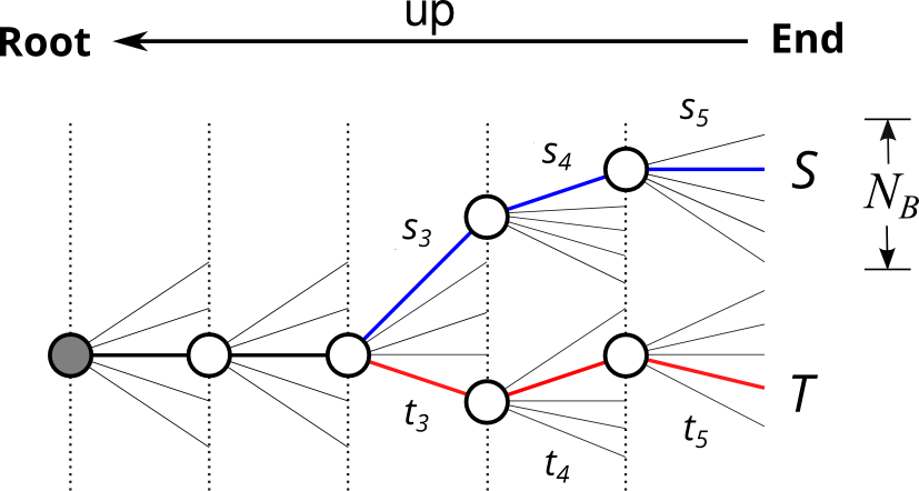
Figure 1: The branching tree of length 5 for the selection of an operator string in a system with a Hamiltonian of $N_{B}$ (here 5) terms. The operator that acts on the state first, is chosen at the first node on the left. This node is called the root and the direction towards the root we define to be up. The operator that acts on the state last is at the end of the string. The two colored paths differ in the choice of the last three operators. The last three branches, thus, contribute different operators and weights ($s_{i}$, $t_{i}$). The resulting strings S and T are different.

As outlined above, VBQMC works by projecting onto the ground-state by repeatedly acting on a trial-state $|\Psi_{T}\rangle$ with $P=c\mathds{1}-H$, where the constant $c$ is chosen such that the ground-state has the biggest eigenvalue. For Hamiltonians with bounded spectrum such a $c$ can always be found. For a simple quantum spin model defined on a lattice we have

$$H=J\sum_{<i,j>}\mathbf{S}_{i}\cdot\mathbf{S}_{j}=\sum_{<i,j>}h_{ij}$$ (1)

and we can write $P=c\mathds{1}-H=\sum O_{ij}$ as a sum over $N_{B}$ bond-operators $O_{ij}$. Taking $P$ to the $n$th power then results in a sum over products of these bond-operators $O_{ij}$:

$$P^{n}=\sum_{a}\underbrace{O_{i(a,1)j(a,1)}\dots O_{i(a,n)j(a,n)}}_{\textrm{$n$-operators}}:=\sum_{a}S_{a}\;.$$ (2)

Each instance of this product then forms a string $S_{a}$ of bond-operators of length $n$. When selecting such a string of length $n$, one has to make a choice between the $N_{B}$ bond-operators at each position in the string. It is possible to view the construction of such a string as a specific path in a decision-tree (see Fig. 1).

Although the algorithms we present can be extended to higher spin models, we shall restrict the discussion to quantum spin models with $S=1/2$ where one usually takes $c=JN_{B}/4$. The action of the bond-operators then takes an attractively simple form.

In a valence bond basis state spins are paired into singlets. A specific pairing of all spins is usually referred to as a covering. All such coverings form an over complete basis for the singlet sub-space of the model. We shall only be concerned with models defined on a bi-partite lattice in which case a given valence bond covering, $C$, for a lattice with $N$ spins can be denoted by listing all $N/2$ pairs of $[i,j]$ with $i$ on sub-lattice $A$ and $j$ on sub-lattice $B$. Here, $[i,j]=(|\uparrow_{i_{A}}\downarrow_{j_{B}}\rangle-|\downarrow_{i_{A}}\uparrow_{j_{B}}\rangle)/\sqrt{2}$. We label the initial covering (trial-state) as $C_{0}$. The action of an operator $O_{ij}$ can take two forms Liang et al. (1988); *liang_existence_1990; Liang (1990b); Sandvik (2005):

• The sites $i$ and $j$ are in a singlet before the action of the operator. Then, the action of the operator does not change the state and we can associate a weight of $w=1$:

  $$O_{ij}[i,j]=1[i,j]\,.$$ (3)

• The sites $i$ and $j$ are not in a singlet before the action of the operator. Then, after the action of the operator, the sites $i$ and $j$ form a singlet. The sites they were originally connected to are also returned in a singlet-state. Furthermore, the state is multiplied by a weight equal to $w=\frac{1}{2}$:

  $$O_{ij}[i,k][l,j]=\frac{1}{2}[i,j][l,k]\,.$$ (4)

A particularly nice feature is that the application of any of the $O_{ij}$ to any given covering yields a unique other covering and not a linear combination of coverings. Although convenient, this feature of projections in the valence bond basis is not strictly necessary for the algorithms we discuss here as they can be adapted to the case where a linear combination of states are generated Deschner and Sørensen (2014). For a given operator string $S_{a}=\prod_{k}O_{k}$, we can associate a weight given by $W_{a}=\prod w_{k}$. The state $S_{a}C_{0}$ will contribute to the final projected estimate of the ground-state with this weight. One can then sample the ground-state by performing a random walk in the space of all possible strings $S_{a}$ Liang et al. (1988); *liang_existence_1990; Liang (1990b); Sandvik (2005) according to the weight $W_{a}$. This way of sampling is quite different from GFMC even though VBQMC and GFMC are closely related projective techniques. GFMC, as it is used in for instance Ref. Runge, 1992, is usually performed in the $S^{z}$ basis but can also be done in terms of the valence bond basis Santoro et al. (1999). In GFMC the projection is done by stochastically evaluating the action of the whole projection-operator on a trial-state. This is done by introducing probabilistic “walkers”. In contrast, as mentioned, in VBQMC a single state results and the strings $S_{a}$ are sampled according to their weight. Clearly, the efficient sampling of states resulting from the stochastic projection of the trial-state is a difficult problem. Here, we propose to use worm (cluster) algorithms for this purpose.

In Monte Carlo calculations one averages over many configurations of the system which are generated with appropriate probabilities. Usually, this is done in a Markov-chain, where one configuration is chosen as a variation of the last. One important feature of an efficient algorithm is that these consecutive configurations are as uncorrelated as possible. This led to the introduction of algorithms where whole clusters and not just single elements are changed going from one configuration to the next Swendsen and Wang (1987); Evertz et al. (1993) or where all elements in the path of a worm are changed Prokof’ev and Svistunov (2001).

Here, we show how it is possible to adapt such worm algorithms for projections in the context of VBQMC. The algorithms we have studied are based on the notion of a worm moving around in the decision tree described above. As in earlier worm algorithms, the change of many elements is achieved by moving the worm based on local conditions Prokof’ev and Svistunov (2001, 2009); Alet and Sørensen (2003a, b); *hitchcock_dual_2004; Wang (2005) and one might refer to the algorithms as tree-worm algorithms. In general, the algorithms can be viewed as directed Alet and Sørensen (2003b); *hitchcock_dual_2004 algorithms.

When we update the string, we start with a worm at the end of the tree and move it up the tree. See Fig. 1. The worm then moves around in the tree and where it goes the operator-string is changed. When the worm finds its way back to the bottom of the tree the update is complete. We derive a set of simple equations governing the movement of the worm. The solution of these equations lead to parameters defining a new class of algorithms. Quite generally, many solutions are possible leaving significant room for choosing parameters that will lead to the most optimal algorithm.

We focus on two specific choices of parameters corresponding to two different algorithms. The bouncing worm algorithm, for which every update is accepted and the driven worm algorithm, for which the update is accepted with some probability. With the driven worm algorithm one can choose at will how much of the operator-string is on average changed in a successful update.

In order to test the algorithms, we calculate the ground-state energy of the isotropic Heisenberg-chain. This quantity is easy to calculate with VBQMC and can be exactly computed using the Bethe-ansatz. It is thus a very convenient quantity to test the algorithms with. The algorithms presented in this paper can, however, be used for the same calculations as other VBQMC implementations (see e.g. Beach and Sandvik (2006)).

In section II we derive the general equations governing the movement of the worm. Section III contains a description of the specific implementation corresponding to the two choices of parameter solutions we have studied. The bouncing worm is detailed in section III.1 while the driven worm algorithm is described in section III.2. The algorithms are then compared in section IV. We present our conclusions in section V.

II Tree Algorithms

We now turn to a discussion of the general framework for the algorithms we have investigated. We begin by deriving the equations governing their behavior in a general way.

Let us take the Hamiltonian to have $N_{B}$ terms. We now imagine a tree where each node indicates the decision to chose one of the $N_{B}$ bond operators composing the string (see Fig. 1). Each branch of the tree corresponds to one of the $N_{B}$ bond operators. A given operator string then corresponds to selecting a path in the tree. Consider 2 such paths S and T that are identical for the part of the operator string first applied to the trial-state. The last 3 operators, however, differ. This leads to different weights, which we denote with $s_{i}$ and $t_{i}$.

As it is done in most Monte Carlo methods, we set out to construct a Markov-chain. Here it is a chain of different strings. If the probabilities to go from one string to the next have detailed balance, the Markov-chain contains the strings with the desired probability. For detailed balance, the probabilities for starting from operator string S and going to operator string T and reverse have to satisfy

$$\frac{P(\textit{{S}}\to\textit{{T}})}{P(\textit{{T}}\to\textsf{{S}})}=\frac{t_{3}t_{4}t_{5}}{s_{3}s_{4}s_{5}}\;.$$ (5)

We can achieve this ratio of probabilities by imagining a worm (tree-worm) working its way up the tree to the point $p$ where it turns around and then working its way down again.

Let us call the valence-bond covering of the trial-state $C_{0}$. Up to numerical factors, the application of an operator string S of length $n$ will yield a new valence-bond covering $\textit{{S}}\,C_{0}\propto C_{n}$. The worm is started by removing the last applied bond operator and considering the resulting covering $C_{n-1}$. A decision now has to be made if the worm is to continue ”up” the tree by removing more bond operators from the string or if it should instead go ”down” the tree by adding a new bond operator to the string. At each node in the tree the decision to continue up or turn around is made according to a set of conditional probabilities $P(\mathrm{up}|s)$ and $P(t|s)$. Here, $P(\mathrm{up}|s)$ denotes the probability for going up after coming from a bond operator that carried weight $s$ and $P(t|s)$ is the probability for turning around by applying a bond operator of weight $t$ coming from an operator with weight $s$. Likewise, $P(s|\mathrm{up})$ denotes the probability of choosing an operator with weight $s$ given that the worm is coming from further up the tree. With these conditional probabilities the left-hand side of Eq. (5) can be written as

$$\frac{P(\textit{{S}}\to\textit{{T}})}{P(\textit{{T}}\to\textsf{{S}})}=\frac{P(t_{5}|\mathrm{up})P(t_{4}|\mathrm{up})P(t_{3}|s_{3})P(\mathrm{up}|s_{4})P(\mathrm{up}|s_{5})}{P(\mathrm{up}|t_{5})P(\mathrm{up}|t_{4})P(s_{3}|t_{3})P(s_{4}|\mathrm{up})P(s_{5}|\mathrm{up})}\;.$$ (6)

Clearly, Eq. (6) is satisfied if we choose

$$\frac{P(\mathrm{up}|s)}{P(s|\mathrm{up})}=\frac{c}{s}\hskip 20.00003pt\textrm{and}\hskip 20.00003pt\frac{P(t|s)}{P(s|t)}=\frac{t}{s}\;,$$ (7)

where $c$ is an additional free parameter included for later optimization of the probabilities. If we can choose conditional probabilities with these properties, we can go between different operator strings always accepting the new string. The rejection probability is then zero. This is a very desirable property of any Monte Carlo Algorithm since it indicates that the algorithm is sampling. We mostly focus on so called zero bounce algorithms for which if the worm turns around the probability for replacing a bond operator with the same operator is zero. Then the two operator strings $S$ and $T$ are always different. This means that

$$P(s|s)=0\,.$$ (8)

Quite generally, it is easy to find many solutions to the equations (7) leading to many Monte Carlo algorithms which can be tuned for efficiency.

We now focus on $S$$=$$1/2$-Heisenberg models defined on bi-partite lattices. As has been described above, for these models only 2 weights can occur: $1,1/2$. The two weights correspond to the two different actions the bond-operators can have on the state. It is $1$ if the operator acts on two sites that are in a valence-bond. The state is not altered under the action of such an operator. We call such operators diagonal. The weight is $1/2$ if the operator acts on two sites that are not in a valence-bond. After the action of the operator the two sites are connected by a bond as well as the sites they were connected to. We call such operators non-diagonal.

If a decision has to be made at the node at position $m$, the conditional probabilities depend on how many of the $N_{B}$ bond-operators will yield a weight of 1 (are diagonal) or $\frac{1}{2}$ (are non-diagonal) when applied to the present covering $C_{m-1}$. We shall denote these numbers by $N_{1}$ and $N_{\frac{1}{2}}$ respectively. When the worm is started $N_{1}$ and $N_{\frac{1}{2}}$ therefore have to be calculated for $C_{n-1}$, if they are not already known from an earlier update. It is thus sensible to store $N_{1}$ or $N_{\frac{1}{2}}$ at all nodes. $N_{1}$ can only be zero at the node furthest up the tree (the root) and only if the trial-state is chosen to not contain any diagonal bonds. In Fig. 1 it is the gray node on the very left. $N_{\frac{1}{2}}$ cannot be smaller than $N_{B}/2$.

We can now write down an $(N_{B}+1)\times(N_{B}+1)$ matrix $M$ of conditional probabilities for each node of the tree. The $j$’th column of the matrix describes the probability for going in any of the $N_{B}+1$ directions when coming from the direction $j$. For clarity we order the rows and columns such that the first $N_{\frac{1}{2}}$ correspond to the non-diagonal operators and the next $N_{1}$ to the diagonal operators. The last column contains the probabilities for going down the tree when coming from above; the last row the probabilities for going up the tree when coming from below. The remaining part of the matrix describe the probabilities for replacing one operator with another when the worm turns from going up to going down. The matrix $M$ has the form

$$\overbrace{\rule{190.63338pt}{0.0pt}}^{N_{\frac{1}{2}}}\overbrace{\rule{146.53151pt}{0.0pt}}^{N_{1}}\overbrace{\rule{51.21504pt}{0.0pt}}^{\mathrm{up}}\rule{11.38092pt}{0.0pt}$$

$$M=\left(\begin{array}[]{ccccccccccccc}P(\frac{1}{2}|\frac{1}{2})&P(\frac{1}{2}^{\prime}|\frac{1}{2})&P(\frac{1}{2}^{\prime}|\frac{1}{2})&\cdots&P(\frac{1}{2}^{\prime}|\frac{1}{2})&\vline&P(\frac{1}{2}|1)&P(\frac{1}{2}|1)&\cdots&P(\frac{1}{2}|1)&\vline&P(\frac{1}{2}|\mathrm{up})\\ P(\frac{1}{2}^{\prime}|\frac{1}{2})&P(\frac{1}{2}|\frac{1}{2})&P(\frac{1}{2}^{\prime}|\frac{1}{2})&\cdots&\cdot&\vline&\cdot&\cdot&\cdots&\cdot&\vline&\cdot\\ \cdot&\cdot&\cdot&&\cdot&\vline&\cdot&\cdot&&\cdot&\vline&\cdot\\ \cdot&\cdot&\cdot&&\cdot&\vline&\cdot&\cdot&&\cdot&\vline&\cdot\\ P(\frac{1}{2}^{\prime}|\frac{1}{2})&P(\frac{1}{2}^{\prime}|\frac{1}{2})&P(\frac{1}{2}^{\prime}|\frac{1}{2})&\cdots&P(\frac{1}{2}|\frac{1}{2})&\vline&P(\frac{1}{2}|1)&P(\frac{1}{2}|1)&\cdots&P(\frac{1}{2}|1)&\vline&P(\frac{1}{2}|\mathrm{up})\\ \hline\cr P(1|\frac{1}{2})&P(1|\frac{1}{2})&P(1|\frac{1}{2})&\cdots&P(1|\frac{1}{2})&\vline&P(1|1)&P(1^{\prime}|1)&\cdots&P(1^{\prime}|1)&\vline&P(1|\mathrm{up})\\ \cdot&\cdot&\cdot&&P(1|\frac{1}{2})&\vline&P(1^{\prime}|1)&P(1|1)&\cdots&\cdot&\vline&\cdot\\ \cdot&\cdot&\cdot&&\cdot&\vline&\cdot&\cdot&&\cdot&\vline&\cdot\\ \cdot&\cdot&\cdot&&\cdot&\vline&\cdot&\cdot&&\cdot&\vline&\cdot\\ P(1|\frac{1}{2})&P(1|\frac{1}{2})&P(1|\frac{1}{2})&\cdots&P(1|\frac{1}{2})&\vline&P(1^{\prime}|1)&P(1^{\prime}|1)&\cdots&P(1|1)&\vline&P(1|\mathrm{up})\\ \hline\cr P(\mathrm{up}|\frac{1}{2})&P(\mathrm{up}|\frac{1}{2})&P(\mathrm{up}|\frac{1}{2})&\cdots&P(\mathrm{up}|\frac{1}{2})&\vline&P(\mathrm{up}|1)&P(\mathrm{up}|1)&\cdots&P(\mathrm{up}|1)&\vline&P(\mathrm{up}|\mathrm{up})\\ \end{array}\right)\;,$$ (20)

where $P(s^{\prime}|s)$ refers to the conditional probability of coming from an operator with weight $s$ and going to a different operator with the same weight. As mentioned above, $P(\mathrm{up}|s)$ denotes the probability for going up coming from an operator with weight $s$ and $P(t|s)$ is the probability for turning around by choosing a bond operator of weight $t$ coming from an operator with weight $s$. Likewise, $P(s|\mathrm{up})$ denotes the probability of choosing an operator with weight $s$ coming from further up the tree.

To shorten the notation we introduce the short-hand

$$x=P({1}/{2}^{\prime}|{1}/{2}),\ \ y=P(1/2|1),\ \ z=P(1^{\prime}|1)\;.$$ (21)

Furthermore we define the ‘bounce’ probabilities

$$b_{\frac{1}{2}}=P(1/2|1/2),\ \ b_{1}=P(1|1),\ \ b_{u}=P(\mathrm{up}|\mathrm{up})\;.$$ (22)

Here it is implied that the probabilities are for going from one operator to the same operator. Finally we also need to define the branching probabilities

$$u=P(1/2|\mathrm{up}),\ \ w=P(1|\mathrm{up})\;,$$ (23)

from which it follows (using Eq. (7)) that:

$$2cu=P(\mathrm{up}|1/2),\ \ cw=P(\mathrm{up}|1)\;.$$ (24)

The matrix $M$ is then given by

$$M=\left(\begin{matrix}b_{\frac{1}{2}}&x&x&\cdots&x&y&y&\cdots&y&u\\ x&b_{\frac{1}{2}}&x&\cdots&x&y&y&\cdots&y&u\\ \cdot&\cdot&\cdot&&\cdot&\cdot&\cdot&&\cdot&\cdot\\ \cdot&\cdot&\cdot&&\cdot&\cdot&\cdot&&\cdot&\cdot\\ x&\cdot&\cdot&\cdots&b_{\frac{1}{2}}&y&y&\cdots&y&u\\ 2y&2y&2y&\cdots&2y&b_{1}&z&\cdots&z&w\\ \cdot&\cdot&\cdot&&2y&z&b_{1}&\cdots&\cdot&\cdot\\ \cdot&\cdot&\cdot&&\cdot&\cdot&\cdot&&\cdot&\cdot\\ \cdot&\cdot&\cdot&&\cdot&\cdot&\cdot&&\cdot&\cdot\\ 2y&2y&2y&\cdots&2y&z&z&\cdots&b_{1}&w\\ 2cu&2cu&2cu&\cdots&2cu&cw&cw&\cdots&cw&b_{u}\\ \end{matrix}\right)\;.$$ (25)

The requirement that this matrix be stochastic (i.e. some branch is chosen with probability one) means that the entries in each column have to sum to 1. This leads to the set of equations

$$1 = N_{\frac{1}{2}}u+N_{1}w+b_{u}$$

$$1 = N_{\frac{1}{2}}y+(N_{1}-1)z+cw+b_{1}$$

$$1 = (N_{\frac{1}{2}}-1)x+N_{1}2y+2cu+b_{\frac{1}{2}}\;.$$ (26)

These simple equations are the central equations governing the behavior of the algorithms. To find an algorithm, we need to solve these 3 equations with the constraints that $0\leq x,y,z,b_{\frac{1}{2}},b_{1},b_{u},u,w\leq 1$; a straight forward problem.

At the root, the equations are modified slightly: since it is not possible to go further up the tree, $2cu$, $cw$, $b_{u}$ are not meaningful and can be set to zero. For convenience we set $b_{1}=x$ and $b_{2}=z$ at the root. This allows one to just choose diagonal operators twice as often as non-diagonal operators. Since the number of diagonal operators does not change at the root, a table generated at the beginning of the calculation suffices to perform this task.

It can be very useful to choose different $c$’s at different nodes. Then, calculating the probabilities to choose operators according to the rules introduced in this section will not lead to an algorithm with detailed balance, because $c_{i}$ from different strings will not cancel in Eq. (6). It is necessary to work with an acceptance probability. We find

$$\frac{P(\textit{{S}}\to\textit{{T}})}{P(\textit{{T}}\to\textsf{{S}})}=\frac{t_{3}t_{4}t_{5}}{s_{3}s_{4}s_{5}}\frac{c^{\textit{{S}}}_{4}c^{\textit{{S}}}_{5}}{c^{\textit{{T}}}_{4}c^{\textit{{T}}}_{5}}\frac{P_{\mathrm{acc}}(\textit{{S}}\to\textit{{T}})}{P_{\mathrm{acc}}(\textit{{T}}\to\textsf{{S}})}\;.$$ (27)

Here $c^{\textit{{S}}}_{i}$ and $c^{\textit{{T}}}_{i}$ denote $c$ at the different nodes in the strings S and T, respectively. To validate the algorithm, we must therefore introduce an acceptance probability that must cancel the factor $(c^{\textit{{S}}}_{4}c^{\textit{{S}}}_{5})/(c^{\textit{{T}}}_{4}c^{\textit{{T}}}_{5})$. This can be achieved by choosing

$$P_{acc}(\textit{{S}}\to\textit{{T}})=\min\Big{(}1,\frac{c^{\textit{{T}}}_{4}c^{\textit{{T}}}_{5}}{c^{\textit{{S}}}_{4}c^{\textit{{S}}}_{5}}\Big{)}\;,$$ (28)

meaning that when a new string is generated through a worm move it is accepted with this probability.

Since we always start from the bottom of the tree (the last operator applied), the worm algorithms presented in this paper always change a block of consecutive branches at the end of the string. This is favorable to changes across the whole string because changes far up the string might be undone by changes closer to the end of the string Sandvik and Beach (2007). In this way the most important part of the string is updated most substantially.

It is also important to note that the algorithm will conserve certain topological numbers. For instance, for a two-dimensional system $S=1/2$ Heisenberg model the number of valence bond crossing a cut in the $x$- or $y$-direction is either odd or even. Hence, the initial covering, $C_{0}$ is characterized by these 2 parities. It is easy to see that the application of $P$ to any covering can not change these parities and they are therefore preserved under the projection.

III Implementations of tree worm algorithms

As is explained in the last section, many different algorithms can be found because many different solutions to the equations (26) exist.

In this section we present two different algorithms. One pure worm algorithm where every update is accepted (the bouncing worm algorithm) and an algorithm that allows for control over how far in the tree updates are attempted (the driven worm algorithm). To test and compare the different algorithms, we calculate the ground-state energy of the antiferromagnetic Heisenberg chain.

The Néel-state $|\textrm{N\'{e}el}\rangle$ has equal overlap with all valence-bond states. This can be used to very directly estimate the ground-state energy, $E_{0}$ Sandvik (2005); *beach_formal_2006; *sandvik_monte_2007:

$$E_{0} =\frac{\langle\textrm{N\'{e}el}|H|\Psi_{0}\rangle}{\langle\textrm{N\'{e}el}|\Psi_{0}\rangle}$$

$$=\lim_{n\to\infty}\frac{\langle\textrm{N\'{e}el}|HP^{n}|C_{0}\rangle}{\langle\textrm{N\'{e}el}|P^{n}|C_{0}\rangle}$$

$$=\lim_{n\to\infty}\sum_{a=1}^{N_{B}^{n}}\frac{\langle\textrm{N\'{e}el}|HS_{a}|C_{0}\rangle}{\sum_{a=1}^{N_{B}^{n}}\langle\textrm{N\'{e}el}|S_{a}|C_{0}\rangle}$$

$$=\lim_{n\to\infty}\sum_{a=1}^{N_{B}^{n}}\frac{W_{a}}{\sum_{a=1}^{N_{B}^{n}}W_{a}}\frac{\langle\textrm{N\'{e}el}|H|C_{a}\rangle}{\langle\textrm{N\'{e}el}|C_{a}\rangle}.$$ (29)

If we take $E_{a}C_{b}=HC_{a}$ and assume that the Monte Carlo sampling will visit strings according to their weight $W_{a}$, then for a Monte Carlo sequence of length $N$ of independent strings we find:

$$E_{0}=\frac{1}{N}\sum_{a=1}^{N}E_{a},$$ (30)

where again we have used the fact that $\langle\textrm{N\'{e}el}|C\rangle$ is independent of the covering $C$.

To analyze the correlation-properties of the worm algorithms we use the energy-autocorrelation-time, which we take to be the number of updates it takes the energy-autocorrelation-function

$$A_{E}(t)=\frac{\langle E_{i}E_{i+t}\rangle-\langle E\rangle^{2}}{\langle E^{2}\rangle-\langle E\rangle^{2}}$$ (31)

to decay to 0.1. The results of all update-attempts enter the calculation of the expectation-values. The shorter the autocorrelation-time is, the fewer steps have to be done between consecutive measurements.

If not stated otherwise an operator-string of 20,000 operators was used for calculations with worm algorithms.

III.1 The bouncing worm algorithm

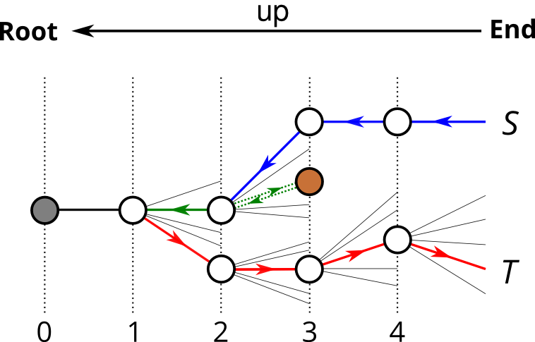
Figure 2: A possible path that contains one bounce and connects the string S and the string T. The worm first goes up to the node $2$ where it turns to go down to node 3. The worm bounces back and goes all the way to node 1. Then the worm turns around and does not bounce again.

The first algorithm we discuss is the bouncing worm algorithm. Only a few of the variables that appear in the equations (26) are chosen to be non-zero. We choose to set:

$$x=y=0,\ \ b_{1}=b_{1/2}=0,$$ (32)

while $z=P(1^{\prime}|1)\neq 0$ as is $u,w$. We leave $b_{u}$ as a parameter that can be zero or non-zero allowing for tuning of the algorithm. With this choice, when the worm is moving up the tree the only possibility for it to turn around is by opting to replace one diagonal operator with another diagonal operator. The $c_{i}$ are chosen to be the same at all nodes: $c_{i}=c$.

The equations for the non-zero parameters are then

$$u = \frac{1}{2c}$$

$$w = \frac{1}{N_{1}}\Big{(}1-\frac{N_{\frac{1}{2}}}{2c}-b_{u}\Big{)}$$

$$z = \frac{1-cw}{N_{1}-1}\;.$$ (33)

The requirements that $z,w>0$ imply that

$$\frac{N_{\frac{1}{2}}}{2(1-b_{u})}\leq c\leq\frac{N_{B}+N_{1}}{2(1-b_{u})}\;.$$ (34)

To satisfy Eq. (34) with node-independent $c$, we set

$$c=\frac{N_{B}}{2(1-b_{u})}\;.$$ (35)

With this choice of parameters, we find the probability to go up the tree if the worm is at a node with a non-diagonal operator to be

$$P(\mathrm{up}|1/2)=2cu=1\,,$$ (36)

for any $b_{u}$. Likewise, if the worm is at a node with a diagonal operator the probability to go up is given by

$$P(\mathrm{up}|1)=cw=1/2\,,$$ (37)

independent of $b_{u}$. The probability for going up the tree is therefore independent of $b_{u}$.

We define the penetration depth (p.-depth), which we denote by $r$, as the maximal height that the worm reaches. The actual length of the worm is denoted by $l$ and with $b_{u}=0$ we find $l=2r$. The penetration depth $r$ will determine how much the operator-string is changed. Obviously, it is desirable to have the worm reach as far up the tree as possible. It is possible to force the worm farther up the tree by having it bounce back to going up after it has turned to go down (see Fig. 2). In that case, the actual length of the worm, $l$, will then be substantially different from twice the penetration depth since the worm can turn many times, a point we shall return to later. Such bounces occurs with a likelihood of $b_{u}$ which was left as a free parameter and can now be used as a tuning parameter.

The algorithm is straight forward to implement and the acceptance probability for a worm update is 1. The move is always accepted. Specific details of an implementation of the bouncing worm update can be found in appendix A.1.

We begin by discussing the case of $b_{u}=0$. In this case the worm first moves up the operator string, turns around once and then proceeds down to the bottom of the tree. It does not go back up the operator string since $b_{u}=0$. In order to measure the performance of the algorithm we did calculations on an antiferromagnetic Heisenberg chain with 50 sites using an operator string of length $100,000$. As can be seen in table 1, this leads to a rather small mean penetration-depth (p.-depth) of about 5. The maximal penetration-depth of 50 is substantially larger. Both these numbers are, however, substantially smaller than the length of the operator string ($100,000$) and it appears that the algorithm with $b_{u}$ is not very effective.

$b_{u}$	mean p.-depth	max p.-depth	slowdown
0.0000	4.561(4)	50	1
0.2500	7.38(1)	305	1.7
0.2750	10.44(3)	1,465	9.7
0.2789	15.64(9)	41,010	316.7
0.2790	19.7(5)	$>$100,000	$<$5,535.7

Table 1: Data for several runs at different $b_{u}$. At $b_{u}\approx 0.25$ increasing the bounce-probability starts to significantly slow down the algorithm. The last column contains the run-times divided by the runtime for $b_{u}$ $=$ $0$. The data were generated with an operator-string of 100,000 operators. The maximal penetration and the expected slowdown could thus not be resolved for $b_{u}$ $=$ $0.2790$. We used $10^{6}$ measurements and a chain with 50 sites.

We now turn to the case $b_{u}\neq 0$. In this case the worm can now switch directions many times during construction (see Fig. 2). The results for the mean and maximal penetration-depth are also listed in table 1. As $b_{u}$ is increased from zero, the maximal penetration-depth first increases very slowly until about $b_{u}=0.25$. It then grows dramatically and, not surprisingly, reaches the length of the operator string. This occurs at $b_{u}\approx 0.2790$. At the same time the mean penetration-depth only increases by a factor of roughly 4, from 5 to about 20. For bounce-probabilities bigger than $b_{u}\approx 1/4$ the program is slowed down significantly compared to the algorithm with $b_{u}=0$ as indicated in the last column in table 1. Thus, even though a large penetration-depth is desirable the computational cost can become so big that increasing $b_{u}$ might not be worthwhile.

In contrast to the maximal penetration-depth, the mean penetration-depth grows very slowly for the values of $b_{u}$ we have been able to study. For computations of reasonable computational cost it never reaches the size of the system and thus also not the length of the operator-string which has to be chosen to be several times the size of the system. That only a small part of the string is updated regularly is directly reflected in the energy-autocorrelation-time (see Fig. 3). The number of bonds that can change in one update of the worm-calculations is twice the penetration-depth. Typical updates never reach far into the operator-string. Thus, the bigger the system is, the less it is perturbed by the update and the more correlated are the energies measured after consecutive updates.

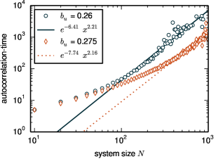
Figure 3: The autocorrelation-time of the energy as a function of system size $N$. The lines indicate tentative power-law fits to the data at large $N$ with a power of $2.21$ for $b_{u}=0.26$ and $2.16$ for $b_{u}=0.275$. Operator-strings of 20,000 operators were used.

As shown in Fig. 3, increasing $b_{u}$ decreases the autocorrelation-time. However, for large system sizes the overall scaling of the autocorrelation-time with the system size appears independent of $b_{u}$. At $b_{u}=0.26$ we find a power-law with an exponent of $2.21$ while a slightly larger $b_{u}=0.275$ yields a power of $2.16$.

Even though the mean penetration depth remains small, one can still obtain high quality results. In particular, it is not necessary for the mean penetration depth to reach a value close to the length of the operator-string (the projection power) in order to get reliable results. Since the maximal penetration-depth is substantially larger than the mean, the operator-string is often updated deeper than the mean penetration-depth. Hence, the mean penetration-depth can be much smaller than the length of the operator-string has to be for otherwise equivalent calculations with conventional VBQMC. We discuss this effect in more detail in section IV.

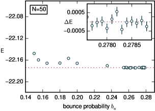
Figure 4: With a bigger probability to bounce $b_{u}$, the bouncing worm algorithm yields a better approximation of the ground-state energy. The ground-state energy was calculated using the Bethe-ansatz and is indicated by a dotted line. Since some operators in the string are never updated, calculations with different $b_{u}$ were effectively done with different trial-states. The calculation was done for a chain with 50 sites. Operator-strings of 20,000 operators were used.

As one increases the probability to bounce up the tree a longer part of the string actually partakes in the projection. Thus, also the quality of the projection is better (see Fig. 4). If operators are never updated, they do not contribute to the projection; they do however modify the trial-state used in the projection. This leads to the irregularly scattered pattern the data shows for small $b_{u}$. In this sense one can think of rare updates that go high up the tree as effectively changing the trial-state and the whole calculation as an averaging over these trial-states.

As is evident from Fig. 4, the bouncing worm algorithm yields good results for $b_{u}>0.25$. It is an attractively simple algorithm with zero bounce probability and a probability of 1 for accepting a new string. The autocorrelation-time can be reduced by increasing $b_{u}$ whereas the overall power of the growth at large system sizes appears independent of $b_{u}$. However, the increased computational cost associated with increasing $b_{u}$ is considerable and we have therefore investigated another parameter choice leading to a different algorithm, the driven worm algorithm. We now turn to a discussion of this algorithm.

III.2 The driven worm algorithm

Clearly, it is desirable to have all updates result in a substantial change of the operator-string. Then, fewer updates have to be performed. For the problem at hand, this means that we need the worm to go far up the tree as often as possible without increasing the computational cost too much. Direct control over the associated probability would be very convenient. We achieve this by setting the probabilities to go up the tree to be

$$2cu=cw=\alpha\,.$$ (38)

The value of $\alpha$ is the probability to, at each node, decide to go up the tree. Since $u$ and $w$ depend on $N_{1}$ and $N_{2}$, this is only possible by allowing $c$ to vary with the node. As explained at the end of section II, the acceptance step of Eq. (28) thus has to be introduced. Updated strings may be rejected.

We set all bounce-probabilities to be zero, $b_{1}=b_{1/2}=b_{u}=0$. Hence, the worm will move up the tree and then turn around once. To get a working algorithm, we have to find solutions to the equations (26) which will determine the transition-probabilities (see Eq. (25)). If $N_{\frac{1}{2}},N_{1}>1$ the solutions to equations (26) are given by:

$$x= \frac{1}{N_{\frac{1}{2}}(N_{\frac{1}{2}}-1)}\Big{[}2N_{1}(N_{1}-1)\ z$$

$$+(1-\alpha)(N_{\frac{1}{2}}-2N_{1})\Big{]}\;,$$

$$y= \frac{1}{N_{\frac{1}{2}}}\Big{[}(1-N_{1})z+1-\alpha\Big{]}\;,$$

$$u= 1/(N_{\frac{1}{2}}+2N_{1})\;,$$

$$w= 2u\;,$$ (39)

where

$$\frac{1-\alpha}{N_{1}-1}\Big{[}1-\frac{N_{\frac{1}{2}}}{2N_{1}}\Big{]}\leq z\leq\frac{1-\alpha}{N_{1}-1}\;.$$ (40)

If $N_{1}\neq 1$, we set

$$z=\frac{1-\alpha}{N_{1}-1}\Big{[}1-\frac{1}{2}\frac{N_{\frac{1}{2}}}{2N_{1}}\Big{]}\ ,$$ (41)

if it results in $z>0$ or

$$z=\frac{1}{2}\frac{1-\alpha}{N_{1}-1}\ \\$$ (42)

otherwise. In this way Eq. (40) is always satisfied and $z\geq 0$. If $N_{1}=1$ we set $z=0$. Finally, we note that the worm update in this case has to be accepted/rejected according to the probability Eq. (28). Specific details of an implementation of this driven worm algorithm can be found in appendix A.2.

How far up the tree updates are attempted can in this case easily be calculated. The probability for the worm to have length $l$ and turn around after going up $r=l/2$ nodes is given by $P(r)=\alpha^{r}(1-\alpha)$. The expectation-value of $r$ is given by

$$\langle r\rangle=\frac{1}{1-\alpha}\;.$$ (43)

The probability distribution for the worm to penetrate the tree $r$ nodes deep during a computation of $m$ updates, is given by

$$P_{m,\alpha}(r_{\textrm{max}})= \underbrace{\Big{(}1-(1-\alpha)\sum_{q=r}^{\infty}\alpha^{q}\Big{)}^{m}}_{\begin{subarray}{c}\text{probability that in $m$ attempts \emph{no} worm}\\ \text{turns at a node with $r>r_{\textrm{max}}$}\end{subarray}}$$

$$-\underbrace{\Big{(}(1-\alpha)\sum_{q=1}^{r-1}\alpha^{q}\Big{)}^{m}}_{\begin{subarray}{c}\text{probability that in $m$ attempts \emph{all} worms}\\ \text{turn at a node with $r<r_{\textrm{max}}$}\end{subarray}}$$

$$= (1-\alpha^{r})^{m}-(1-\alpha^{r-1})^{m}\;.$$ (44)

How far up the tree is updated, is not given by how far the worm goes up the tree since the update might be rejected. The mean penetration-depth is therefore not equal to $\langle r\rangle$. In Fig. 5 we show results for the mean and maximal penetration-depth for two different system sizes, $N=50,1000$ as a function of $1/(1-\alpha)$. As expected, both the mean and maximal penetration-depth increase monotonically with $1/(1-\alpha)$.

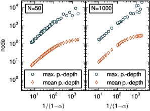
Figure 5: The mean and the maximal penetration-depths grow as $\alpha$ approaches one. The mean penetration-depth is always smaller than $\langle r\rangle=1/(1-\alpha)$. This behavior is independent of the system size. For the chain with 50 sites $\mathrm{3}\times\mathrm{10}^{\mathrm{8}}$ and for the chain with 1000 sites $\mathrm{10}^{\mathrm{7}}$ updates were performed. Operator-strings of 20,000 operators were used.

Another measure of the performance of the algorithm can be established by simply looking at the calculated ground-state energy and its error. This is done in Fig. 6 where the ground-state energy is shown as a function of $1/(1-\alpha)$. Operators that are never updated, only change the effective trial-state the ground-state is projected out of. By forcing the worm further up the tree, one can have a bigger part of the operator-string partake in the projection (see Fig. 5). This leads to a better approximation of the ground-state energy as can be seen in Fig. 6.

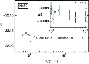
Figure 6: The bigger the penetration probability $\alpha$, the better the approximation of the ground-state energy given by the driven worm algorithm. The ground-state energy was calculated using the Bethe-ansatz. It is indicated by a dotted line. Since some operators in the string are never updated, calculations with different $\alpha$ were effectively done with different trial-states. The calculation was done for a chain with 50 sites. Operator-strings of 20,000 operators were used.

For the driven worm algorithm we have also studied the behavior of the autocorrelation-time of the energy. Our results are shown in Fig. 7 as a function of $1/(1-\alpha)$. The behavior is in this case not monotonic. At first the autocorrelation time decreases, but then it starts to grow at larger $1/(1-\alpha)$.

This can be understood in the following way: As long as $\langle r\rangle$ is much smaller than the size of the system, the autocorrelation-time decreases with increasing $\alpha$. This follows naturally from the fact that increasing $1/(1-\alpha)$ will increase $\langle r\rangle$ and therefore lead to larger and more effective updates. This decreases the correlations between operator-strings. The farther the worm travels up the string, the smaller is the probability that an update is accepted (see table 2). For bigger $\alpha$, and thus also $\langle r\rangle$, this effect dominates and the autocorrelation-time grows. A characteristic minimum in the autocorrelation-time as $1/(1-\alpha)$ is increased can then be identified as is clearly evident in Fig. 7.

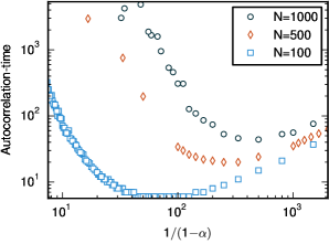
Figure 7: The autocorrelation-time decreases with $\langle r\rangle$, if typical updates are smaller than the system size. Since bigger $\langle r\rangle$ means better projection, this implies that the autocorrelation-time decreases as the quality of the projection is improved. Operator-strings of 20,000 operators were used.

$1/(1-\alpha)$	acceptance-rate
200	0.41
1000	0.13
5000	0.03

Table 2: The acceptance rate drops when the string is updated more substantially. The calculations were done for a chain with 50 sites.

IV Comparison of algorithms

In the following we compare worm-updates to simple conventional VBQMC-updates as described for example in reference Sandvik and Beach (2007). This means that for VBQMC we attempt to change 4 randomly selected operators during one update. We do not compare to loop-updates as introduced in reference Sandvik and Evertz (2010), since we anticipate the worm algorithms to be of most with algorithms for which loop-updates are not known although our current implementations of them are similar to conventional VBQMC.

We first consider the convergence of the energy with the projection power (the length of the operator strings). Our results for a 50 site Heisenberg chain are shown in Fig. 8. It turns out that if the worm algorithms penetrate the tree sufficiently deeply, the results do not depend on the type of algorithm in use. In particular, the dependence of the results on the length of the string is the same for all three algorithms (see Fig. 8), just as one might have expected since the power method underlies all three algorithms.

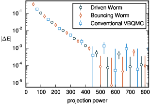
Figure 8: Upon increasing the quality of the projection by using longer operator strings, the estimate of the ground-state energy converges to the correct value in the same way for worm- and conventional VBQMC-algorithm as long as the string is penetrated sufficiently deeply. The driven worm algorithm was run with the probability to go up the tree $\alpha=0.995$, which corresponds to a mean penetration-depth of about $90$ and full penetration of the string. The bouncing worm algorithm was run with a bounce probability $b_{u}=0.2675$, which corresponds to a mean penetration-depth of roughly $8$ and full penetration of the string. The calculation was done for a chain with 50 sites.

When using the worm algorithms, the operator string is usually chosen so long that the worm never or very rarely reaches the root of the tree. This means that there are almost always nodes close to the root with operators that are never updated and thus act on the trial-state after every update. In this way, we are effectively using an optimized trial-state. The effect is similar to generating the trial-state by performing several updates on a randomly chosen trial-state and taking the resulting state for the actual calculation. We used such a trial-state for the conventional VBQMC-calculations shown in this section.

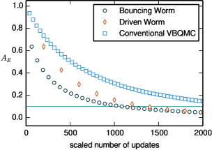
Figure 9: The autocorrelation-function versus scaled number of updates for the two worm algorithms and conventional VBQMC. The number of updates was scaled by the number of operators attempted to be changed in an update, $\langle l/2\rangle$. Hence, data for conventional VBQMC updates, the driven worm algorithm and the bouncing worm algorithm were multiplied by $4$, $200$ and $63.758$, respectively. For the worm algorithms the same parameters as in Fig. 8 were used. This means that $\alpha=0.995$ and $b_{u}=0.2675$. An operator-string of length 1000 was used for all three algorithms. The horizontal line at $0.1$ was added to allow for easy visual estimation of the scaled autocorrelation-time.

A useful measure of the effectiveness of an algorithm can be obtained from the autocorrelation function. If simply measured as a function of the number of updates it decreases dramatically faster for the worm algorithms when compared to conventional VBQMC. However, just using one update as the temporal unit puts conventional VBQMC at an unfair disadvantage. The reason is, that in calculations with conventional VBQMC one attempts to change 4 operators per update while for the worm algorithms it could be many more. The number of updated operators in a given worm update varies greatly with the length of the worm, $\langle l\rangle$, which can easily be hundreds of operators long. Since a single worm update is, therefore, computationally more expensive to perform than a single 4 operator update with conventional VBQMC, it seems fairer to compare autocorrelation functions with this difference taken into account. That is, a fair comparison would ask which algorithm has the smallest correlations when on average the same number of changes has been attempted. We can take this into account by simply scaling the temporal axis with the average size of the attempted update.

In Fig. 9 we therefore show results for the energy autocorrelation function for the two worm algorithms as well as for conventional VBQMC with the temporal axis rescaled by the number of operators one attempts to change in a single update. During one update with worm-algorithms one tries to update $l/2$ operators. The scaled number of updates is simply $\#\mathrm{updates}\times\langle l/2\rangle$ with $\langle l/2\rangle=4$ for conventional VBQMC and $\langle l/2\rangle=\langle r\rangle=1/(1-\alpha)$ for the driven worm algorithm. For the bouncing worm algorithm, $\langle l\rangle$ has to be measured during the simulation, since the bouncing worm can go up and down the tree many times. Thus, $\langle l/2\rangle$ can be orders of magnitudes bigger than the mean penetration-depth. For instance, for the calculations shown in Fig. 9 the mean penetration-depth was approximately 7.8 whereas $\langle l/2\rangle=63.758$. Even including such a rescaling of the temporal axis, it is clear that the autocorrelation-times are much shorter for the worm algorithms, as shown in Fig. 9.

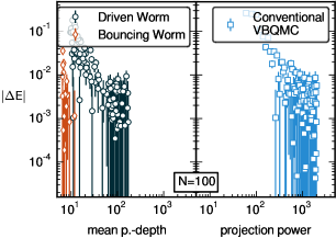
Figure 10: The deviation, $|\Delta E|$, from the exact Bethe-ansatz results for a chain with 100 sites. The results are shown for the driven and bouncing worm algorithms versus the mean penetration-depth and for conventional VBQMC updates versus the projective power (length of operator string). The worm algorithms reach the same small value of $|\Delta E|$ with a mean penetration-depth an order of magnitude smaller than the projective power used for the calculation with conventional VBQMC updates. The bars on the markers indicated the statistical uncertainty. The colored (dark) surfaces are due to overlapping error-bars. Operator-strings of 20,000 operators were used for the calculations with the worm algorithms.

The two worm algorithms change operators of the string starting from one end while the conventional VBQMC selects 4 operators at random to be changed. As mentioned in subsection III.1, the mean and the maximum penetration-depth are usually much smaller than the length of the operator-string (the projection power). It is therefore natural to ask if one can reach a similar quality of results using worm algorithms and conventional VBQMC.

That this is so can be seen by plotting the absolute deviation from the ground-state energy, $|\Delta E|$, versus the mean penetration-depth. As shown in Fig. 10, the mean penetration-depth can, in fact, be much smaller than the projection power of a conventional VBQMC-calculation and still yield results of the same accuracy.

Finally, we look at how the scaled autocorrelation-time depends on the size of the system studied. For convenience, we define the scaled autocorrelation-time to be the point where the autocorrelation function has decreased to the value $0.1$ (see Fig. 9). Since in realistic calculations one would use a fixed (large) length of operator string with the worm algorithms, while one would scale it with the size of the system in conventional VBQMC, we here only compare the two worm algorithms. Our results are shown in Fig. 11 for a fixed length operator string of $20,000$.

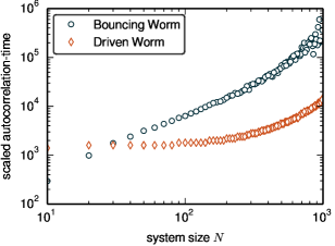
Figure 11: The scaled autocorrelation-time for the driven and bouncing worm algorithms as a function of system size. A fixed operator string of length $20,000$ was used in the calculations. In the calculations shown, the bouncing worm algorithm was run with $b_{u}=0.275$ and the driven worm algorithm was run with $\alpha=0.995$. For the scaling we use $\langle l/2\rangle=200$ for the driven worm algorithm and an $\langle l/2\rangle$ between $60$ for $N=10$ and $221$ for $N=1000$ for the bouncing worm algorithm.

For the simulations shown in Fig. 11 the mean penetration-depths for the driven worm algorithm were about $100$. The autocorrelation-time for the driven worm algorithm starts to increase appreciably at this system size, while it is initially are almost flat. We conclude that a significant increase in the autocorrelation-time appears once the system size significantly exceeds the mean penetration-depth. A similar effect can be observed for the bouncing worm algorithm. The mean penetration-depths for the bouncing worm algorithm are, however, much smaller (around $9$; see Fig. 10). Results for $N$ smaller than the mean penetration-depth are therefore not shown in Fig. 11. The autocorrelation-times remain manageable for the system sizes studied, even though it is consistently increasing.

Compared to simple implementations of VBQMC, the worm algorithms have significant overhead. This is largely compensated by the large number of operators that can be changed in an update and resulting shorter autocorrelation-times, as we found in all computations. Given the somewhat different properties of the two worm algorithms, a realistic implementation could combine the two by performing updates with the driven worm algorithm mixed with updates using the bouncing worm algorithm (and perhaps conventional VBQMC updates).

V Conclusion

We have shown that valence-bond quantum Monte Carlo can be implemented with an update build around the notion of a worm propagating through a tree. Many different such algorithms are possible. We studied the validity and efficiency of two of them. One for which no update is rejected (the bouncing worm algorithm) and one for which big parts of the operator-string are updated (the driven worm algorithm). Both algorithms are attractively simple and straight forward to implement and produce high quality results.

While they may not be computationally competitive with state of the art loop update algorithms Sandvik and Evertz (2010) for VBQMC, the algorithms presented here are intrinsically interesting since they represent a new class of algorithms that should be generally applicable to projective methods. These algorithms are not restricted to the valence bond basis and preliminary results show that they can be quite efficient in the $S^{z}$-basis Deschner and Sørensen (2014) method and might spark further development of it. We also note that many other algorithms can easily be found with the results contained in this paper and that it is possible that the parameter space allows for much more efficient algorithms than the two we have studied here.

In terms of further optimizing the algorithms several directions may be interesting to pursue. Not updating some of the operators the worm visits, might boost the acceptance ratio of the driven worm algorithms and thereby reduce the autocorrelation-times. This could be combined with attempting to reduce the overhead of the driven worm calculations by always forcing the worm all the way down to the root. This would eliminate the need to keep track of the state at each node. With the current practice of updating all operators after turning around, going all the way to the node during every update leads to very small acceptance ratios.

We acknowledge computing time at the Shared Hierarchical Academic Research Computing Network (SHARCNET:www.sharcnet.ca) and research support from NSERC.

Appendix A Pseudocode for implementations of the tree worm algorithm

This appendix contains pseudocode that shall serve to clarify the algorithms proposed in this paper. To simplify notation we refer to diagonal operator as DOP and non-diagonal operators as NDOP.

A.1 Bouncing worm algorithm

In this section we give detailed information on a straightforward (albeit not optimized) implementation of the bounce-algorithm (see Subsec. III.1). Shown is an outline of the central part of the algorithm: the update of the operator-string and the state.

The algorithm works its way up the tree. It starts at the last branch which is assigned the $n$th position. At each position it is decided if the worm goes up the tree or down, in which case a new operator is chosen for the branch at this position. The necessary probabilities are calculated according to the expressions given in Eq. 33 and Eq. 35. If a new operator is chosen for the $n$th branch, the update is complete.

It is assumed that the tree is so high (the operator-string so long) that the root is never reached. If the root is reached, one has to choose an operator for the first branch according to the probabilities outlined in Sec. II after Eq. 26.

Schematically, using pseudocode, a bouncing worm update of a tree with $n$ nodes can be outlined as follows:

$\mathtt{pos}=n$ $\triangleright$ start at last branch $\mathtt{going\_up}=$ TRUE while $\mathtt{pos}\;!=n+1$ do      $\mathtt{ran}=\mathrm{uniform(0,1)}$      if $\mathtt{going\_up}$ then          if operator at $\mathtt{pos}$ is NDOP then               $\mathtt{pos}=\mathtt{pos}-1$          else if $\mathtt{ran}<cw$ then               $\mathtt{pos}=\mathtt{pos}-1$          else               $\mathtt{going\_up}=$ FALSE               choose new DOP at $\mathtt{pos}$               update state, $w$ and $N_{1}$ at $\mathtt{pos}$               $\mathtt{pos}=\mathtt{pos}+1$          end if      else          if $\mathrm{ran}<b_{u}$ then               $\mathtt{going\_up}=$ TRUE          else               if $\mathtt{ran}-b_{u}<wN_{1}$ then                   choose DOP at $\mathtt{pos}$               else                   choose NDOP at $\mathtt{pos}$               end if               update state, $w$ and $N_{1}$ at $\mathtt{pos}$               $\mathtt{pos}=\mathtt{pos}+1$          end if      end if end while

The weights $w,u$ and $b_{u}$, $N_{1}$ as well as the state are stored at each node.

A.2 Driven worm algorithm

We now turn to a description of a (not optimized) implementation of the driven worm algorithm (see Subsec. III.2). As above, we show an outline of the central part of the algorithm: the update of the operator-string and the state.

The worm works its way up the tree. It starts at the last branch which is assigned the position $n$. While going up the tree, the worm, at each node, goes further up the tree with probability $\alpha$ or turns around with probability $1$$-$$\alpha$. After turning around, the worm keeps going down until it reaches the end. At the nodes the worm visits new operators are chosen. When the worm reaches the end, it has to be decided whether or not the update should be accepted. The associated probabilities are calculated according to the expressions given in the main text (see Eq. 38, Eq. III.2 and Eq. 28).

As above, we assume that the tree is so high (the operator-strings so long) that the root is never reached. If that the root is reached, one has to choose an operator for the first branch according to the probabilities outlined in Sec. II after Eq. 26.

Shown is the driven worm update of a tree with $n$ nodes. Using pseudocode language, a driven worm update then takes the following form for a tree with $n$ nodes:

$\mathtt{pos}=n$ $\triangleright$ start at last branch $\mathtt{going\_up}=$ TRUE while $\mathtt{pos}\;!=n+1$ do      $\mathtt{ran}=\mathrm{uniform(0,1)}$      while $\mathtt{going\_up}$ do          if $\mathtt{ran}<\alpha$ then               $\mathtt{pos}=\mathtt{pos}-1$          else               $\mathtt{going\_up}=$ FALSE               if operator at $\mathtt{pos}$ is DOP then                   if $\mathtt{ran}-\alpha<yN_{1/2}$ then                        choose new NDOP at $\mathtt{pos}$                   else                        choose DOP at $\mathtt{pos}$                   end if               else                   if $\mathtt{ran}-\alpha<zN_{1}$ then                        choose new DOP at $\mathtt{pos}$                   else                        choose NDOP at $\mathtt{pos}$                   end if                   update state, weights, $c$, and $N_{1}$ at $\mathtt{pos}$                   $\mathtt{pos}=\mathtt{pos}+1$               end if          end if      end while      if $\mathtt{ran}<wN_{1}$ then          choose DOP at $\mathtt{pos}$      else          choose NDOP at $\mathtt{pos}$      end if      update state, weights, $c$, and $N_{1}$ at $\mathtt{pos}$      $\mathtt{pos}=\mathtt{pos}+1$ end while Accept or reject using old and new $c$’s.

The weights, $c$, $N_{1}$ as well as the state are stored at each node. A new string is not always accepted.

References

- Ceperley and Kalos (1986) D. Ceperley and M. Kalos, in Monte Carlo Methods in Statistical Physics, Topics in Current Physics, Vol. 7, edited by K. Binder (Springer Berlin Heidelberg, 1986) pp. 145–194.
- Blankenbecler and Sugar (1983) R. Blankenbecler and R. L. Sugar, Physical Review D 27, 1304 (1983).
- Liang et al. (1988) S. Liang, B. Doucot, and P. W. Anderson, Phys. Rev. Lett. 61, 365 (1988).
- Liang (1990a) S. Liang, Phys. Rev. B 42, 6555 (1990a).
- Liang (1990b) S. Liang, Phys. Rev. Lett. 64, 1597 (1990b).
- Trivedi and Ceperley (1990) N. Trivedi and D. M. Ceperley, Physical Review B 41, 4552 (1990).
- Runge (1992) K. J. Runge, Physical Review B 45, 7229 (1992).
- Calandra et al. (1998) M. Calandra, F. Becca, and S. Sorella, Physical Review Letters 81, 5185 (1998).
- Capriotti et al. (1999) L. Capriotti, A. E. Trumper, and S. Sorella, Physical Review Letters 82, 3899 (1999).
- von der Linden (1992) W. von der Linden, Physics Reports 220, 53 (1992).
- Cerf and Martin (1995) N. J. Cerf and O. C. Martin, International Journal of Modern Physics C 06, 693 (1995).
- Sorella et al. (2013) S. Sorella, G. E. Santoro, and F. Becca, “SISSA Lecture notes on Numerical methods for strongly correlated electrons,” (2013).
- Hetherington (1984) J. H. Hetherington, Physical Review A 30, 2713 (1984).
- Sandvik (2005) A. W. Sandvik, Phys. Rev. Lett. 95, 207203 (2005).
- Beach and Sandvik (2006) K. Beach and A. W. Sandvik, Nuclear Physics B 750, 142 (2006).
- Sandvik and Beach (2007) A. W. Sandvik and K. S. D. Beach, 0704.1469 (2007).
- Sandvik and Evertz (2010) A. W. Sandvik and H. G. Evertz, Phys. Rev. B 82, 024407 (2010).
- Banerjee and Damle (2010) A. Banerjee and K. Damle, Journal of Statistical Mechanics: Theory and Experiment 2010, P08017 (2010).
- Deschner and Sørensen (2014) A. Deschner and E. S. Sørensen, unpublished (2014).
- Santoro et al. (1999) G. Santoro, S. Sorella, L. Guidoni, A. Parola, and E. Tosatti, Physical Review Letters 83, 3065 (1999).
- Swendsen and Wang (1987) R. H. Swendsen and J.-S. Wang, Phys. Rev. Lett. 58, 86 (1987).
- Evertz et al. (1993) H. G. Evertz, G. Lana, and M. Marcu, Phys. Rev. Lett. 70, 875 (1993).
- Prokof’ev and Svistunov (2001) N. Prokof’ev and B. Svistunov, Phys. Rev. Lett. 87 (2001).
- Prokof’ev and Svistunov (2009) N. Prokof’ev and B. Svistunov, Worm Algorithm for Problems of Quantum and Classical Statistics, arXiv e-print 0910.1393 (2009).
- Alet and Sørensen (2003a) F. Alet and E. S. Sørensen, Phys. Rev. E 67, 015701 (2003a).
- Alet and Sørensen (2003b) F. Alet and E. S. Sørensen, Phys. Rev. E 68, 026702 (2003b).
- Hitchcock et al. (2004) P. Hitchcock, E. S. Sørensen, and F. Alet, Phys. Rev. E 70, 016702 (2004).
- Wang (2005) J.-S. Wang, Phys. Rev. E 72, 036706 (2005).