Mie scattering of Laguerre-Gaussian beams: photonic nanojets and near-field optical vortices

Abstract

We study Mie light scattering of Laguerre-Gaussian (LG) beams remodelled using the method of far-field matching. The theoretical results are applied to examine the optical field in the near-field region for purely azimuthal LG beams characterized by the nonzero azimuthal mode number $m_{\mathrm{LG}}$. The mode number $m_{\mathrm{LG}}$ is found to have a profound effect on the morphology of photonic nanojets and the near-field structure of optical vortices associated with the components of the electric field.

I Introduction

The problem of light scattering by particles of one medium embedded in another has a long history, dating back more than a century to the classical exact solution due to Mie Mie (1908). The Mie solution applies to scattering by uniform spherical particles with isotropic dielectric properties. The analysis of a Mie–type theory uses a systematic expansion of the electromagnetic field over vector spherical harmonics Newton (1982); Bohren and Huffman (1983); Tsang et al. (2000); Mishchenko et al. (2004); Doicu et al. (2006); Gouesbet and Gréhan (2011). The specific form of the expansions is also known as the T–matrix ansatz that has been widely used in the related problem of light scattering by nonspherical particles Mishchenko et al. (1996, 2000, 2004). More recently this strategy has been successfully applied to optically anisotropic particles  Roth and Digman (1973); Lange and Aragon (1990); Hahn and Aragon (1994); Karacali et al. (1997); Kiselev et al. (2000, 2002a); Geng et al. (2004); Novitsky and Barkovsky (2008); Qiu et al. (2010).

In its original form the Mie theory assumes that the scatterer is illuminated with a plane electromagnetic wave. For laser beams, it is generally necessary to go beyond the plane-wave approximation that may severely break down when the beam width becomes of order of the scatterer size. The problem of light scattering from arbitrary shaped laser beams has now a more than two decade long history Grehan et al. (1986); Gouesbet et al. (1988a); Barton et al. (1988, 1989); Schaub et al. (1992) and has been the key subject of the Mie–type theory — the so-called generalized Lorenz–Mie theory (GLMT)  Lock and Gouesbet (2009); Gouesbet and Gréhan (2011) — extended to the case of arbitrary incident-beam scattering.

Mathematically, in such generalization of the Mie theory, the central and the most important task is to describe illuminating beams in terms of expansions over a set of basis wavefunctions (for the spherical coordinate system, it is the multipole expansion over the basis of vector spherical wavefunctions). In GLMT, a variety of formally exact (the quadrature and double quadrature formulas) and approximate (the finite series and localized approximations) methods Gouesbet et al. (1988b) were developed to evaluate the expansion coefficients that are referred to as the beam shape coefficients (for a recent review see Ref. Gouesbet et al. (2011) and references therein).

The central problem with laser beams is due to the fact that in their standard mathematical form these beams are not radiation fields which are solutions to Maxwell’s equations. Typically, the analytical treatment of laser beams is performed using the paraxial approximation Lax et al. (1975) and the beams are described as pseudo-fields which are only approximate solutions of the vector Helmholtz equation (higher order corrections can be used to improve the accuracy of the paraxial approximation Lax et al. (1975); Davis (1979)).

Unfortunately, multipole expansions do not exist for such approximate pseudo-fields. Therefore, some remodelling procedure must be invoked to obtain a real radiation field which can be regarded as an approximation to the original paraxial beam.

The basic concept that might be called matching the fields on a surface lies at the heart of various traditional approaches to the laser beam remodelling and is based on the assumption that there is a surface where the actual incident field is equal to the paraxial field. Examples of physically reasonable and natural choice are scatterer-independent matching surfaces such as a far-field sphere Nieminen et al. (2003), the focal plane (for beams with well-defined focal planes) Nieminen et al. (2003); Bareil and Sheng (2013), and a Gaussian reference sphere representing a lens Hoang et al. (2012). Given the paraxial field distribution on the matching surface, the beam shape coefficients can be evaluated using either numerical integration or the one-point matching method Nieminen et al. (2003).

An alternative approach is to describe analytically propagation of a laser beam, which is known in the paraxial limit, without recourse to the paraxial approximation. In Refs. Barnett and Allen (1994); Duan et al. (2005); Van De Nes et al. (2006); Zhou (2006, 2008) this strategy has been applied to the important case of Laguerre–Gaussian (LG) beams using different methods such as the vectorial Rayleigh–Sommerfeld formulas Duan et al. (2005); Zhou (2008), the vector angular spectrum method Zhou (2006), approximating LG beams by nonparaxial beams with (near) cylindrical symmetry Barnett and Allen (1994); Van De Nes et al. (2006).

The nonparaxial beams are solutions of Maxwell’s equations and the beam shape coefficients can be computed using the methods of GLMT. In recent studies of light scattering by spherical and spheroidal particles illuminated with LG beams van de Ness and Török (2007); Jiang et al. (2012), the analytical results of Ref. Van De Nes et al. (2006) were used to calculate the beam shape coefficients.

It is now well known Allen et al. (2003) that LG beams represent optical vortex beams that carry angular momentum of two kinds: spin angular momentum associated with the polarization state of the beam and orbital angular momentum related to spatial variations of the field. These variations derive from the helical structure of the wavefronts comprising the beam or, equivalently, from a phase singularity at the beam axis. The topological charge characterizing the phase singularity and associated orbital angular momentum gives rise to distinctive phenomena such as soliton generation Desyatnikov et al. (2005), entanglement of photon quantum states, orbital angular momentum exchange with atoms and molecules (in addition to the collection of papers Allen et al. (2003), see reviews in Ref. Andrews (2008)), rotation and orbital motion of spherical particles illuminated with LG beams Simpson and Hanna (2009, 2010).

In this paper the problem of light scattering from LG beams that represent laser beams exhibiting a helical phase front and carrying a phase singularity will be of our primary interest. In our calculations we shall follow Ref. Kiselev et al. (2002a) and use the $T$–matrix approach in which the far-field matching method is combined with the results for nonparaxial propagation of LG beams Zhou (2006, 2008). Our goal is to examine the near-field structure of electromagnetic field depending on the parameters characterizing both the beam and the scatterer.

This structure has recently attracted considerable attention that was stimulated by an upsurge of interest to the so-called photonic nanojets and their applications (for a review see Ref. Heifetz et al. (2009)). These nanojets were originally identified in finite-difference-time-domain simulations Chen et al. (2004); Li et al. (2005) as narrow, high-intensity electromagnetic beams that propagate into background medium from the shadow-side surface of a plane-wave illuminated dielectric microcylinder Chen et al. (2004) or microsphere Li et al. (2005) of diameter greater than the illuminating wavelength. In other words, a photonic nanojet can be regarded as a localized, subdiffractional, non-evanescent light focus propagating along the line of incidence.

The bulk of theoretical studies devoted to nanojets Lecler et al. (2005); Devilez et al. (2008); Geints et al. (2010); Ding et al. (2010); Geints et al. (2012); Guo et al. (2013) has been predominantly focused on the case of plane-wave illumination. In this paper we intend to fill the gap.

The layout of the paper is as follows. In Sec. II, we describe our theoretical approach and then, in Sec. III, we obtain the analytical results for the beam shape coefficients of LG beams. The numerical procedure and the results of numerical computations representing the near-field intensity distributions and phase maps of electric field components for purely azimuthal LG beams are presented in Sec. IV.

Finally, in Sec. V, we present our results and make some concluding remarks.

II T–matrix formulation of Lorenz–Mie theory

We consider scattering by a spherical particle of radius $R_{p}$ embedded in a uniform isotropic dielectric medium with dielectric constant $\epsilon_{\mathrm{med}}$ and magnetic permeability $\mu_{\mathrm{med}}$. The dielectric constant and magnetic permittivity of the particle are $\epsilon_{p}$ and $\mu_{p}$, respectively.

In this subsection we remind the reader about the relationship between Maxwell’s equations in the region of a scatterer and the formulation of scattering properties in terms of the T–matrix Newton (1982); Mishchenko et al. (2004). Our formulation is slightly non-standard and closely follows to the line of our presentation given in Ref. Kiselev et al. (2002a).

We shall need to write the Maxwell equations for a harmonic electromagnetic wave (time–dependent factor is $\exp\{-i\omega t\}$) in the form:

$$-ik_{i}^{-1}\,\boldsymbol{\nabla}\times\mathbf{E} =\frac{\mu_{i}}{n_{i}}\mathbf{H}\,,$$ (1a)

$$ik_{i}^{-1}\,\boldsymbol{\nabla}\times\mathbf{H} =\frac{n_{i}}{\mu_{i}}\mathbf{E},\quad i=\begin{cases}\mathrm{med},&r>R_{p}\\ p,&r<R_{p}\end{cases}$$ (1b)

where $n_{\mathrm{med}}=\sqrt{\epsilon_{\mathrm{med}}\mu_{\mathrm{med}}}$ is the refractive index outside the scatterer (in the ambient medium), where $r>R_{p}$ ($i=\mathrm{med}$) and $k_{i}=k_{\mathrm{med}}=n_{\mathrm{med}}k_{\mathrm{vac}}$ ($k_{\mathrm{vac}}=\omega/c=2\pi/\lambda$ is the free–space wavenumber); $n_{p}=\sqrt{\epsilon_{p}\mu_{p}}$ is the refractive index for the region inside the spherical particle (scatterer), where $r<R_{p}$ ($i=p$) and $k_{i}=k_{p}=n_{p}k_{\mathrm{vac}}$.

II.1 Vector spherical harmonics and Wigner D functions

The electromagnetic field can always be expanded using the vector spherical harmonic basis, $\mathbf{Y}_{j+\delta\,j\,m}(\phi,\theta)\equiv\mathbf{Y}_{j+\delta\,j\,m}(\hat{\mathbf{r}})$ ($\delta=0,\pm 1$) Biedenharn and Louck (1981), as follows:

$$\mathbf{E}=\sum_{jm}\mathbf{E}_{jm}=\sum_{jm}\left[p^{(0)}_{jm}(r)\mathbf{Y}^{(0)}_{jm}(\hat{\mathbf{r}})+p^{(e)}_{jm}(r)\mathbf{Y}^{(e)}_{jm}(\hat{\mathbf{r}})+p^{(m)}_{jm}(r)\mathbf{Y}^{(m)}_{jm}(\hat{\mathbf{r}})\right]\>,$$ (2a)

$$\mathbf{H}=\sum_{jm}\mathbf{H}_{jm}=\sum_{jm}\left[q^{(0)}_{jm}(r)\mathbf{Y}^{(0)}_{jm}(\hat{\mathbf{r}})+q^{(e)}_{jm}(r)\mathbf{Y}^{(e)}_{jm}(\hat{\mathbf{r}})+q^{(m)}_{jm}(r)\mathbf{Y}^{(m)}_{jm}(\hat{\mathbf{r}})\right]\>,$$ (2b)

where $\mathbf{Y}^{(m)}_{jm}=\mathbf{Y}_{j\,j\,m}$ and $\mathbf{Y}^{(e)}_{jm}=[j/(2j+1)]^{1/2}\mathbf{Y}_{j+1\,j\,m}+[(j+1)/(2j+1)]^{1/2}\mathbf{Y}_{j-1\,j\,m}$ are electric and magnetic harmonics respectively, and $\mathbf{Y}^{(0)}_{jm}=[j/(2j+1)]^{1/2}\mathbf{Y}_{j-1\,j\,m}-[(j+1)/(2j+1)]^{1/2}\mathbf{Y}_{j+1\,j\,m}$ are longitudinal harmonics. In Ref. Kiselev et al. (2002a), it was shown that the spherical harmonics can be conveniently expressed in terms of the Wigner D–functions Biedenharn and Louck (1981); Varshalovich et al. (1988) as follows

$$\mathbf{Y}_{jm}^{(m)}(\hat{\mathbf{r}})=N_{j}/\sqrt{2}\left\{D_{m,\,-1}^{j\,*}(\hat{\mathbf{r}})\,\mathbf{e}_{-1}(\hat{\mathbf{r}})-D_{m,\,1}^{j\,*}(\hat{\mathbf{r}})\,\mathbf{e}_{+1}(\hat{\mathbf{r}})\right\}\,,$$ (3a)

$$\mathbf{Y}_{jm}^{(e)}(\hat{\mathbf{r}})=N_{j}/\sqrt{2}\left\{D_{m,\,-1}^{j\,*}(\hat{\mathbf{r}})\,\mathbf{e}_{-1}(\hat{\mathbf{r}})+D_{m,\,1}^{j\,*}(\hat{\mathbf{r}})\,\mathbf{e}_{+1}(\hat{\mathbf{r}})\right\}\,,$$ (3b)

$$\mathbf{Y}_{jm}^{(0)}(\hat{\mathbf{r}})=N_{j}D_{m,\,0}^{j\,*}(\hat{\mathbf{r}})\,\mathbf{e}_{0}(\hat{\mathbf{r}})=Y_{jm}(\hat{\mathbf{r}})\hat{\mathbf{r}},\quad N_{j}=[(2j+1)/4\pi]^{1/2},$$ (3c)

where $\mathbf{e}_{\pm 1}(\hat{\mathbf{r}})=\mp(\mathbf{e}_{x}(\hat{\mathbf{r}})\pm i\mathbf{e}_{y}(\hat{\mathbf{r}}))/\sqrt{2}$; $\mathbf{e}_{x}(\hat{\mathbf{r}})\equiv\hat{\boldsymbol{\vartheta}}=(\cos\theta\cos\phi,\cos\theta\sin\phi,-\sin\theta)$, $\mathbf{e}_{y}(\hat{\mathbf{r}})\equiv\hat{\boldsymbol{\varphi}}=(-\sin\phi,\cos\phi,0)$ are the unit vectors tangential to the sphere; $\phi$ ($\theta$) is the azimuthal (polar) angle of the unit vector $\hat{\mathbf{r}}=\mathbf{r}/r=(\sin\theta\cos\phi,\sin\theta\sin\phi,\cos\theta)\equiv\mathbf{e}_{0}(\hat{\mathbf{r}})\equiv\mathbf{e}_{z}(\hat{\mathbf{r}})$. (Hats will denote unit vectors and an asterisk will indicate complex conjugation.)

Note that, for the irreducible representation of the rotation group with the angular number $j$, the D-functions, $D_{m\nu}^{\,j}(\alpha,\beta,\gamma)=\exp(-im\alpha)d_{m\mu}^{\,j}(\beta)\exp(-i\mu\gamma)$, give the elements of the rotation matrix parametrized by the three Euler angles Biedenharn and Louck (1981); Varshalovich et al. (1988): $\alpha$, $\beta$ and $\gamma$. In formulas (3) and throughout this paper, we assume that $\gamma=0$ and $D_{m\nu}^{\,j}(\hat{\mathbf{r}})\equiv D_{m\nu}^{\,j}(\phi,\theta,0)$. These D-functions meet the following orthogonality relations Biedenharn and Louck (1981); Varshalovich et al. (1988)

$$\langle D_{m\nu}^{\,j\,*}(\hat{\mathbf{r}})D_{m^{\prime}\nu}^{\,j^{\prime}}(\hat{\mathbf{r}})\rangle_{\hat{\mathbf{r}}}=\frac{4\pi}{2j+1}\,\delta_{jj^{\prime}}\,\delta_{mm^{\prime}}\,,$$ (4)

where $\displaystyle\langle\,f\,\rangle_{\hat{\mathbf{r}}}\equiv\int_{0}^{2\pi}\mathrm{d}\phi\int_{0}^{\pi}\sin\theta\mathrm{d}\theta\,f(\hat{\mathbf{r}})$ and $f(\hat{\mathbf{r}})\equiv f(\phi,\theta)$. The orthogonality condition (4) and Eqs. (3) show that a set of vector spherical harmonics is orthonormal:

$$\langle\mathbf{Y}_{jm}^{(\alpha)\,*}(\hat{\mathbf{r}})\cdot\mathbf{Y}_{j^{\prime}m^{\prime}}^{(\beta)}(\hat{\mathbf{r}})\rangle_{\hat{\mathbf{r}}}=\delta_{\alpha\beta}\,\delta_{jj^{\prime}}\,\delta_{mm^{\prime}}\,.$$ (5)

We can now use the relations Biedenharn and Louck (1981)

$$N_{j}D_{m\,0}^{\,j\,*}(\hat{\mathbf{r}})=\mathrm{Y}_{jm}(\hat{\mathbf{r}}),$$ (6)

$$N_{j}D_{m\,\pm 1}^{\,j\,*}(\hat{\mathbf{r}})=n_{j}\left[\mp\partial_{\theta}+\frac{i}{\sin\theta}\partial_{\phi}\right]\mathrm{Y}_{jm}(\hat{\mathbf{r}}),\quad n_{j}\equiv[j(j+1)]^{-1/2}$$ (7)

where $\partial_{x}$ stands for a derivative with respect to $x$ and $\mathrm{Y}_{jm}(\hat{\mathbf{r}})$ is the normalized spherical function

$$\mathrm{Y}_{jm}(\phi,\theta)=N_{j}\exp(im\phi)d^{\,j}_{m,0}(\theta)=(-1)^{m}\sqrt{\frac{(2j+1)(j-m)!}{4\pi(j+m)!}}\,\exp(im\phi)\,P_{j}^{\,m}(\cos\theta)$$ (8)

expressed in terms of the associated Legendre polynomial of degree $j$ and order $m$

$$P_{j}^{\,m}(x)=\begin{cases}(-1)^{m}/(2^{j}j!)(1-x^{2})^{m/2}\partial_{x}^{j+m}(x^{2}-1)^{j},&m>0\\ (-1)^{|m|}(j-|m|)!/(j+|m|)!P_{j}^{\,|m|}(x),&m<0\end{cases},$$ (9)

and derive the following expressions for the magnetic and electric vector spherical functions

$$\mathbf{Y}_{jm}^{(m)}(\hat{\mathbf{r}})=-in_{j}\left[[\partial_{\theta}\mathrm{Y}_{jm}]\hat{\boldsymbol{\varphi}}-i\frac{m}{\sin\theta}\mathrm{Y}_{jm}\hat{\boldsymbol{\vartheta}}\right]=$$

$$n_{j}\mathbf{L}\mathrm{Y}_{jm}=-i\hat{\mathbf{r}}\times\mathbf{Y}_{jm}^{(e)},$$ (10)

$$\mathbf{Y}_{jm}^{(e)}(\hat{\mathbf{r}})=n_{j}\left[[\partial_{\theta}\mathrm{Y}_{jm}]\hat{\boldsymbol{\vartheta}}+i\frac{m}{\sin\theta}\mathrm{Y}_{jm}\hat{\boldsymbol{\varphi}}\right]=$$

$$n_{j}r\boldsymbol{\nabla}\mathrm{Y}_{jm}=-i\hat{\mathbf{r}}\times\mathbf{Y}_{jm}^{(m)},$$ (11)

where $\mathbf{L}$ is the operator of angular momentum given by

$$i\mathbf{L}=\mathbf{r}\times\boldsymbol{\nabla}=\hat{\boldsymbol{\varphi}}\,\partial_{\theta}-\hat{\boldsymbol{\vartheta}}\,[\sin\theta]^{-1}\partial_{\phi}.$$ (12)

Formulas (II.1) and (II.1) give the vector spherical harmonics (3) rewritten in the well-known standard form Jackson (1999).

II.2 Wave functions and T–matrix

The electric field (2a) is completely described by the coefficients $\{p_{jm}^{(\lambda)}(r)\}$ and similarly the magnetic field (2b) is described by $\{q_{jm}^{(\lambda)}(r)\}$ with $\lambda=\{0,e,m\}$. In order to find the coefficient functions we can use separation of variables. This implies that the expansions (2) must be inserted into Maxwell’s equations (1). The coefficient functions then can be derived by solving the resulting system of equations. In the simplest case of an isotropic medium the coefficient functions can be expressed in terms of spherical Bessel functions, $j_{j}(x)=[\pi/(2x)]^{1/2}J_{j+1/2}(x)$, and spherical Hankel functions Abramowitz and Stegun (1972), $h_{j}^{(1,\,2)}(x)=[\pi/(2x)]^{1/2}H_{j+1/2}^{(1,\,2)}(x)$, and their derivatives.

Alternatively, it is well-known (a discussion of the procedure can be found, e.g., in Ref. Sarkar and Halas (1997)) that solutions of the scalar Helmholtz equation, $(\boldsymbol{\nabla}^{2}+k^{2})\psi(\mathbf{r})=0$, taken in the form

$$\psi_{jm}^{(\alpha)}=n_{j}z_{j}^{(\alpha)}(\rho)\mathrm{Y}(\hat{\mathbf{r}}),\quad n_{j}\equiv[j(j+1)]^{-1/2},$$ (13)

where $\rho=kr$ and $z_{j}^{(\alpha)}(\rho)$ is either a spherical Bessel or Hankel function, can be used to obtain the following solenoidal solutions of the vector Helmholtz equation, $\boldsymbol{\nabla}\times[\boldsymbol{\nabla}\times\boldsymbol{\Psi}]=k^{2}\boldsymbol{\Psi}$:

$$\mathbf{M}_{jm}^{(\alpha)}(\rho,\hat{\mathbf{r}})=\mathbf{L}\psi_{jm}^{(\alpha)}=z_{j}^{(\alpha)}(\rho)\mathbf{Y}_{jm}^{(m)}(\hat{\mathbf{r}}),$$ (14)

$$\mathbf{N}_{jm}^{(\alpha)}(\rho,\hat{\mathbf{r}})=-ik^{-1}\,\boldsymbol{\nabla}\times\mathbf{M}_{jm}^{(\alpha)}=\frac{\sqrt{j(j+1)}}{\rho}\,z_{j}^{(\alpha)}(\rho)\,\mathbf{Y}_{jm}^{(0)}(\hat{\mathbf{r}})+Dz_{j}^{(\alpha)}(\rho)\mathbf{Y}_{jm}^{(e)}(\hat{\mathbf{r}}),$$ (15)

where $Df(x)\equiv x^{-1}\partial_{x}(xf(x))$. The vector wave functions, $\mathbf{M}_{jm}^{(\alpha)}$ and $\mathbf{N}_{jm}^{(\alpha)}$, are linked through the identities

$$-i\boldsymbol{\nabla}\times\mathbf{M}_{jm}^{(\alpha)}=k\mathbf{N}_{jm}^{(\alpha)},\quad i\boldsymbol{\nabla}\times\mathbf{N}_{jm}^{(\alpha)}=k\mathbf{M}_{jm}^{(\alpha)}$$ (16)

and their linear combination represents the expansions (2) over the vector spherical harmonics.

There are three cases of these expansions that are of particular interest. They correspond to the incident wave, $\{\mathbf{E}_{\mathrm{inc}},\mathbf{H}_{\mathrm{inc}}\}$, the outgoing scattered wave, $\{\mathbf{E}_{\mathrm{sca}},\mathbf{H}_{\mathrm{sca}}\}$ and the electromagnetic field inside the scatterer, $\{\mathbf{E}_{p},\mathbf{H}_{p}\}$:

$$\mathbf{E}_{\alpha}=\sum_{jm}\bigl{[}\alpha_{jm}^{(\alpha)}\mathbf{M}_{jm}^{(\alpha)}(\rho_{i},\hat{\mathbf{r}})+\beta_{jm}^{(\alpha)}\mathbf{N}_{jm}^{(\alpha)}(\rho_{i},\hat{\mathbf{r}})\bigr{]},\quad\alpha\in\{\mathrm{inc},\mathrm{sca},p\}$$ (17a)

$$\mathbf{H}_{\alpha}=n_{i}/\mu_{i}\sum_{jm}\bigl{[}\alpha_{jm}^{(\alpha)}\mathbf{N}_{jm}^{(\alpha)}(\rho_{i},\hat{\mathbf{r}})-\beta_{jm}^{(\alpha)}\mathbf{M}_{jm}^{(\alpha)}(\rho_{i},\hat{\mathbf{r}})\bigr{]},$$ (17b)

$$i=\begin{cases}\mathrm{med},&\alpha\in\{\mathrm{inc},\mathrm{sca}\}\\ p,&\alpha=p\end{cases},\quad z_{j}^{(\alpha)}(\rho_{i})=\begin{cases}j_{j}(\rho),&\alpha=\mathrm{inc}\\ h_{j}^{(1)}(\rho),&\alpha=\mathrm{sca}\\ j_{j}(\rho_{p}),&\alpha=p\\ \end{cases},$$ (17c)

where $\rho_{\mathrm{med}}=k_{\mathrm{med}}r\equiv\rho$, $\rho_{p}=k_{p}r\equiv n\rho$, and $n=n_{p}/n_{\mathrm{med}}$ is the ratio of refractive indexes also known as the optical contrast.

Thus outside the scatterer the electromagnetic field is a sum of the incident wave field with $z_{j}^{(\mathrm{inc})}(\rho)=j_{j}(\rho)$ and the scattered waves with $z_{j}^{(\mathrm{sca})}(\rho)=h_{j}^{(1)}(\rho)$ as required by the Sommerfeld radiation condition.

In the far field region ($\rho\gg 1$), the asymptotic behaviour of the spherical Bessel and Hankel functions is known Abramowitz and Stegun (1972):

$$i^{j+1}h_{j}^{(1)}(\rho),i^{j}Dh_{j}^{(1)}(\rho)\sim\exp(i\rho)/\rho,$$ (18)

$$(-i)^{j+1}h_{j}^{(2)}(\rho),(-i)^{j}Dh_{j}^{(2)}(\rho)\sim\exp(-i\rho)/\rho,$$ (19)

$$i^{j+1}j_{j}(\rho),i^{j+1}Dj_{j+1}(\rho)\sim\bigl{[}\exp(i\rho)-(-1)^{j}\exp(-i\rho)\bigr{]}/(2\rho).$$ (20)

So, the spherical Hankel functions of the first kind, $h_{j}^{(1)}(\rho)$, describe the outgoing waves, whereas those of the second kind, $h_{j}^{(2)}(\rho)$, represent the incoming waves.

The incident field is the field that would exist without a scatterer and therefore includes both incoming and outgoing parts (see Eq. (20)) because, when no scattering, what comes in must go outwards again. As opposed to the spherical Hankel functions that are singular at the origin, the incident wave field should be finite everywhere and thus is described by the regular Bessel functions $j_{j}(\rho)$.

Now the incident wave is characterized by amplitudes $\alpha_{jm}^{(\mathrm{inc})}$, $\beta_{jm}^{(\mathrm{inc})}$ and the scattered outgoing waves are similarly characterized by amplitudes $\alpha_{jm}^{(\mathrm{sca})}$, $\beta_{jm}^{(\mathrm{sca})}$. So long as the scattering problem is linear, the coefficients $\alpha_{jm}^{(\mathrm{sca})}$ and $\beta_{jm}^{(\mathrm{sca})}$ can be written as linear combinations of $\alpha_{jm}^{(\mathrm{inc})}$ and $\beta_{jm}^{(\mathrm{inc})}$:

$$\alpha_{jm}^{(\mathrm{sca})}=\sum_{j^{\prime},m^{\prime}}\left[\,T_{jm,\,j^{\prime}m^{\prime}}^{\,11}\,\alpha_{j^{\prime}m^{\prime}}^{(\mathrm{inc})}+T_{jm,\,j^{\prime}m^{\prime}}^{\,12}\,\beta_{j^{\prime}m^{\prime}}^{(\mathrm{inc})}\,\right],$$

$$\beta_{jm}^{(\mathrm{sca})}=\sum_{j^{\prime},m^{\prime}}\left[\,T_{jm,\,j^{\prime}m^{\prime}}^{\,21}\,\alpha_{j^{\prime}m^{\prime}}^{(\mathrm{inc})}+T_{jm,\,j^{\prime}m^{\prime}}^{\,22}\,\beta_{j^{\prime}m^{\prime}}^{(\mathrm{inc})}\,\right]\,.$$ (21)

These formulae define the elements of the T–matrix in the most general case.

In general, the outgoing wave with angular momentum index $j$ arises from ingoing waves of all other indices $j^{\prime}$. In such cases we say that the scattering process mixes angular momenta Mishchenko et al. (1996). The light scattering from uniformly anisotropic scatterers Kiselev et al. (2002a, b) provides an example of such a scattering process. In simpler scattering processes, by contrast, such angular momentum mixing does not take place. Many quantum scattering processes and classical Mie scattering belong to this category. For example, radial anisotropy keeps intact spherical symmetry of the scatterer Roth and Digman (1973); Kiselev et al. (2002a); Qiu et al. (2010). The T–matrix of a spherically symmetric scatterer is diagonal over the angular momenta and the azimuthal numbers: $T_{jj^{\prime},mm^{\prime}}^{nn^{\prime}}=\delta_{jj^{\prime}}\delta_{mm^{\prime}}T_{j}^{nn^{\prime}}$.

In order to calculate the elements of T-matrix and the coefficients $\alpha_{jm}^{(p)}$ and $\beta_{jm}^{(p)}$, we need to use continuity of the tangential components of the electric and magnetic fields as boundary conditions at $r=R_{p}$ ($\rho=k_{\mathrm{med}}R_{p}\equiv x$).

So, the coefficients of the expansion for the wave field inside the scatterer, $\alpha_{jm}^{(p)}$ and $\alpha_{jm}^{(p)}$, are expressed in terms of the coefficients describing the incident light as follows

$$i\alpha_{jm}^{(p)}=\frac{\alpha_{jm}^{(\mathrm{inc})}}{\mu^{-1}v_{j}(x)u_{j}^{\prime}(nx)-n^{-1}v_{j}^{\prime}(x)u_{j}(nx)},\quad\mu=\mu_{p}/\mu_{\mathrm{med}},$$ (22)

$$i\beta_{jm}^{(p)}=\frac{\beta_{jm}^{(\mathrm{inc})}}{n^{-1}v_{j}(x)u_{j}^{\prime}(nx)-\mu^{-1}v_{j}^{\prime}(x)u_{j}(nx)},\quad n=n_{p}/n_{\mathrm{med}},$$ (23)

where $x=k_{\mathrm{med}}R_{p}$, $u_{j}(x)=xj_{j}(x)$ and $v_{j}(x)=xh_{j}^{(1)}(x)$. The similar result relating the scattered wave and the incident wave

$$\alpha_{jm}^{(\mathrm{sca})}=T_{j}^{11}\alpha_{jm}^{(\mathrm{inc})}=\frac{n^{-1}u_{j}^{\prime}(x)u_{j}(nx)-\mu^{-1}u_{j}(x)u_{j}^{\prime}(nx)}{\mu^{-1}v_{j}(x)u_{j}^{\prime}(nx)-n^{-1}v_{j}^{\prime}(x)u_{j}(nx)}\alpha_{jm}^{(\mathrm{inc})},$$ (24)

$$\beta_{jm}^{(\mathrm{sca})}=T_{j}^{22}\beta_{jm}^{(\mathrm{inc})}=\frac{\mu^{-1}u_{j}(x)u_{j}^{\prime}(nx)-n^{-1}u_{j}^{\prime}(x)u_{j}(nx)}{n^{-1}v_{j}(x)u_{j}^{\prime}(nx)-\mu^{-1}v_{j}^{\prime}(x)u_{j}(nx)}\beta_{jm}^{(\mathrm{inc})},$$ (25)

defines the T-matrix for the simplest case of a spherically symmetric scatterer. In addition, since the parity of electric and magnetic harmonics with respect to the spatial inversion $\hat{\mathbf{r}}\to-\hat{\mathbf{r}}$ ($\{\phi,\theta\}\to\{\phi+\pi,\pi-\theta\}$) is different

$$\mathbf{Y}_{jm}^{(m)}(-\hat{\mathbf{r}})=(-1)^{j}\mathbf{Y}_{jm}^{(m)}(\hat{\mathbf{r}}),\quad\mathbf{Y}_{jm}^{(e)}(-\hat{\mathbf{r}})=(-1)^{j+1}\mathbf{Y}_{jm}^{(e)}(\hat{\mathbf{r}}),$$ (26)

where $f(\hat{\mathbf{r}})\equiv f(\phi,\theta)$ and $f(-\hat{\mathbf{r}})\equiv f(\phi+\pi,\pi-\theta)$, they do not mix provided the mirror symmetry has not been broken. In this case the T-matrix is diagonal and $T_{j}^{12}=T_{j}^{21}=0$. The diagonal elements $T_{j}^{11}$ and $T_{j}^{22}$ are also called the Mie coefficients.

III Incident wave beams

The formulas (22)- (25) are useful only if the expansion for the incident light beam is known. First we briefly review the most studied and fundamentally important case where the incident light is represented by a plane wave.

III.1 Plane waves

The electric field of a transverse plane wave propagating along the direction specified by a unit vector $\hat{\mathbf{k}}_{\mathrm{inc}}$ is

$$\mathbf{E}_{\mathrm{inc}}=\mathbf{E}^{(\mathrm{inc})}\exp(i\,\mathbf{k}_{\mathrm{inc}}\cdot\mathbf{r})\,,\quad\mathbf{E}^{(\mathrm{inc})}=\sum_{\nu=\pm 1}E_{\nu}^{(\mathrm{inc})}\mathbf{e}_{\nu}(\hat{\mathbf{k}}_{\mathrm{inc}})\,,\qquad\mathbf{k}_{\mathrm{inc}}=k\hat{\mathbf{k}}_{\mathrm{inc}}\,.$$ (27)

where the basis vectors $\mathbf{e}_{\pm 1}(\hat{\mathbf{k}}_{\mathrm{inc}})$ are perpendicular to $\hat{\mathbf{k}}_{\mathrm{inc}}$. Then the vector version of the well known Rayleigh expansion (see, for example, Newton (1982))

$$\exp(i\,\rho\hat{\mathbf{k}}\cdot\hat{\mathbf{r}})=4\pi\sum_{l=0}^{\infty}\sum_{m=-l}^{l}i^{\,l}j_{l}(\rho)\,Y_{lm}(\hat{\mathbf{r}})\,Y_{lm}^{*}(\hat{\mathbf{k}}),\quad\rho\equiv kr$$ (28)

which is given by

$$\mathbf{e}_{\nu}(\hat{\mathbf{k}})\exp[i\rho\bigl{(}{\hat{\mathbf{k}}}\cdot{\hat{\mathbf{r}}}\bigr{)}]=\sum_{jm}\alpha_{j}D_{m\nu}^{\,j}(\hat{\mathbf{k}})\Bigl{\{}i\nu\mathbf{M}_{jm}(\rho,\hat{\mathbf{r}})-\mathbf{N}_{jm}(\rho,\hat{\mathbf{r}})\Bigr{\}},\quad\nu=\pm 1,$$ (29)

where $\alpha_{j}=i^{j+1}[2\pi(2j+1)]^{1/2}$, immediately gives the expansion coefficients for the plane wave

$$\alpha_{jm}^{(\mathrm{inc})} =i\alpha_{j}\sum_{\nu=\pm 1}D_{m\nu}^{j}(\hat{\mathbf{k}}_{\mathrm{inc}})\nu E_{\nu}^{(\mathrm{inc})},\quad\beta_{jm}^{(\mathrm{inc})}=-\alpha_{j}\sum_{\nu=\pm 1}D_{m\nu}^{j}(\hat{\mathbf{k}}_{\mathrm{inc}})E_{\nu}^{(\mathrm{inc})}\,,$$ (30)

where $D_{mm^{\prime}}^{j}$ is the Wigner $D$-function.

In the far field region, the electric field of scattered wave is related to the polarization vector of the plane wave through the scattering amplitude matrix as follows Newton (1982); Ishimaru (1978); Mishchenko et al. (1996)

$$E_{\nu}^{(\mathrm{sca})}\equiv(\mathbf{e}_{\nu}^{\,*}(\hat{\mathbf{k}}_{\mathrm{sca}}),\mathbf{E}_{\mathrm{sca}})=\rho^{-1}\exp(i\rho)\sum_{\nu^{\prime}=\pm 1}\mathbf{A}_{\nu\nu^{\prime}}(\hat{\mathbf{k}}_{\mathrm{sca}},\hat{\mathbf{k}}_{\mathrm{inc}})E_{\nu^{\prime}}^{(\mathrm{inc})}\,,\quad\nu=\pm 1\,$$ (31)

where $\hat{\mathbf{k}}_{\mathrm{sca}}=\hat{\mathbf{r}}$. For a spherically symmetric scatterer, the expression for the scattering amplitude matrix in terms of T-matrix is given by

$$\mathbf{A}_{\nu\nu^{\prime}}(\hat{\mathbf{k}}_{\mathrm{sca}},\hat{\mathbf{k}}_{\mathrm{inc}}) =\sum_{j}\mathbf{A}_{\nu\nu^{\prime}}^{j}(\hat{\mathbf{k}}_{\mathrm{sca}},\hat{\mathbf{k}}_{\mathrm{inc}})=$$

$$= -i\sum_{j}(j+1/2)\tilde{D}_{\nu\nu^{\prime}}^{j}(\hat{\mathbf{k}}_{\mathrm{sca}},\hat{\mathbf{k}}_{\mathrm{inc}})\,\left[\,\nu\nu^{\prime}\,T_{j}^{\,11}-i\nu\,T_{j}^{\,12}+i\nu^{\prime}\,T_{j}^{\,21}+T_{j}^{\,22}\,\right]\,,$$ (32a)

$$\tilde{D}_{\nu\nu^{\prime}}^{j}(\hat{\mathbf{k}}_{\mathrm{sca}},\hat{\mathbf{k}}_{\mathrm{inc}})=\sum_{m}D_{m\nu}^{j\,*}(\hat{\mathbf{k}}_{\mathrm{sca}})D_{m\nu^{\prime}}^{j}(\hat{\mathbf{k}}_{\mathrm{inc}})\,.$$ (32b)

Equation (32b) shows that the scattering amplitude matrix (32a) depends only on the angle between $\hat{\mathbf{k}}_{\mathrm{inc}}$ and $\hat{\mathbf{k}}_{\mathrm{sca}}$. All far-field scattering characteristics of the system can be computed from the scattering amplitude matrix.

III.2 Far-field matching

Now we consider a more general case where an incident electromagnetic wave is written as a superposition of propagating plane waves:

$$\mathbf{E}_{\mathrm{inc}}(\mathbf{r})\equiv\mathbf{E}_{\mathrm{inc}}(\rho,\hat{\mathbf{r}})=\langle\exp(i\rho\,\hat{\mathbf{k}}\cdot\hat{\mathbf{r}})\,\mathbf{E}_{\mathrm{inc}}(\hat{\mathbf{k}})\rangle_{\hat{\mathbf{k}}},\quad\mathbf{E}_{\mathrm{inc}}(\hat{\mathbf{k}})=\sum_{\nu=\pm 1}E_{\nu}(\hat{\mathbf{k}})\,\mathbf{e}_{\nu}(\hat{\mathbf{k}}),$$ (33a)

$$\mathbf{H}_{\mathrm{inc}}(\mathbf{r})\equiv\mathbf{H}_{\mathrm{inc}}(\rho,\hat{\mathbf{r}})=\frac{n}{\mu}\,\langle\exp(i\rho\,\hat{\mathbf{k}}\cdot\hat{\mathbf{r}})\,\bigl{[}\hat{\mathbf{k}}\times\mathbf{E}_{\mathrm{inc}}(\hat{\mathbf{k}})\bigr{]}\rangle_{\hat{\mathbf{k}}}\,,$$ (33b)

where $\displaystyle\langle\,f\,\rangle_{\hat{\mathbf{k}}}\equiv\int_{0}^{2\pi}\mathrm{d}\phi_{k}\int_{0}^{\pi}\sin\theta_{k}\mathrm{d}\theta_{k}\,f$.

Our first step is to examine asymptotic behavior of the wave field (33) in the far-field region, $\rho\gg 1$. The results can be easily obtained by using the asymptotic formula for a plane wave (see, e.g., Mishchenko et al. (2004))

$$\exp(i\rho\,\hat{\mathbf{k}}\cdot\hat{\mathbf{r}})\sim\frac{-2\pi i}{\rho}\bigl{[}\exp(i\rho)\delta(\hat{\mathbf{k}}-\hat{\mathbf{r}})-\exp(-i\rho)\delta(\hat{\mathbf{k}}+\hat{\mathbf{r}})\bigr{]}\quad\text{ at }\rho\gg 1,$$ (34)

where $\delta(\hat{\mathbf{k}}\mp\hat{\mathbf{r}})$ is the solid angle Dirac $\delta$-function symbolically defined through the expansion

$$\delta(\hat{\mathbf{k}}\mp\hat{\mathbf{r}})=\sum_{l=0}^{\infty}\sum_{m=-l}^{l}Y_{lm}(\pm\hat{\mathbf{r}})\,Y_{lm}^{*}(\hat{\mathbf{k}}).$$ (35)

Applying the relation (34) to the plane wave superposition (33a) gives the electric field of the incident wave in the far-field region

$$\mathbf{E}_{\mathrm{inc}}(\rho,\hat{\mathbf{r}})\sim\mathbf{E}_{\mathrm{inc}}^{(\infty)}(\rho,\hat{\mathbf{r}})=\frac{1}{\rho}\bigl{[}\exp(i\rho)\mathbf{E}_{\mathrm{out}}(\hat{\mathbf{r}})+\exp(-i\rho)\mathbf{E}_{\mathrm{in}}(\hat{\mathbf{r}})\bigr{]},$$ (36)

$$\mathbf{E}_{\mathrm{in}}(\hat{\mathbf{r}})=-\mathbf{E}_{\mathrm{out}}(-\hat{\mathbf{r}}),$$ (37)

where $\mathbf{E}_{\mathrm{out}}(\hat{\mathbf{r}})$ is the far-field angular distribution for the outgoing part of the electric field of the incident wave:

$$\mathbf{E}_{\mathrm{out}}(\hat{\mathbf{r}})=-2\pi i\,\mathbf{E}_{\mathrm{inc}}(\hat{\mathbf{r}})=E_{\theta}^{(\mathrm{out})}(\hat{\mathbf{r}})\,\mathbf{e}_{\theta}(\hat{\mathbf{r}})+E_{\phi}^{(\mathrm{out})}(\hat{\mathbf{r}})\,\mathbf{e}_{\phi}(\hat{\mathbf{r}}),$$ (38)

whereas the incoming part of the incident wave is described by the far-field angular distribution $\mathbf{E}_{\mathrm{in}}(\hat{\mathbf{r}})$.

The result for the far-field distribution of the magnetic field (33b) can be written in the similar form:

$$\mathbf{H}_{\mathrm{inc}}(\rho,\hat{\mathbf{r}})\sim\mathbf{H}_{\mathrm{inc}}^{(\infty)}(\rho,\hat{\mathbf{r}})=\frac{1}{\rho}\bigl{[}\exp(i\rho)\mathbf{H}_{\mathrm{out}}(\hat{\mathbf{r}})+\exp(-i\rho)\mathbf{H}_{\mathrm{in}}(\hat{\mathbf{r}})\bigr{]},$$ (39)

$$\mathbf{H}_{\mathrm{in}}(\hat{\mathbf{r}})=-\mathbf{H}_{\mathrm{out}}(-\hat{\mathbf{r}}),$$ (40)

$$\mu/n\,\mathbf{H}_{\mathrm{out}}(\hat{\mathbf{r}})=\hat{\mathbf{r}}\times\mathbf{E}_{\mathrm{out}}(\hat{\mathbf{r}}),\quad\mu/n\,\mathbf{H}_{\mathrm{in}}(\hat{\mathbf{r}})=\hat{\mathbf{r}}\times\mathbf{E}_{\mathrm{out}}(-\hat{\mathbf{r}}).$$ (41)

Formulas (36)-(41) explicitly show that, in the far-field region, the incident wave field is defined by the angular distribution of the outgoing wave (38). In particular, from these formulas, it is not difficult to obtain the far-field expression for the Poynting vector of the incident wave $\mathbf{S}_{\mathrm{inc}}=c/(8\pi)\mathop{\rm Re}\nolimits(\mathbf{E}_{\mathrm{inc}}\times\mathbf{H}_{\mathrm{inc}}^{\,*})$

$$\mathbf{S}_{\mathrm{inc}}(\rho,\hat{\mathbf{r}})\sim\mathbf{S}_{\mathrm{inc}}^{(\infty)}(\rho,\hat{\mathbf{r}})=\rho^{-2}\bigl{\{}\mathbf{S}_{\mathrm{in}}(\hat{\mathbf{r}})+\mathbf{S}_{\mathrm{out}}(\hat{\mathbf{r}})\bigr{\}},$$ (42)

$$\mathbf{S}_{\mathrm{in}}(\hat{\mathbf{r}})=-\mathbf{S}_{\mathrm{out}}(-\hat{\mathbf{r}}),\quad\mu/n\,\mathbf{S}_{\mathrm{out}}(\hat{\mathbf{r}})=c/(8\pi)\,|\mathbf{E}_{\mathrm{out}}(\hat{\mathbf{r}})|^{2}\,\hat{\mathbf{r}},$$ (43)

where $|\mathbf{E}_{\mathrm{out}}(\hat{\mathbf{r}})|^{2}=(\mathbf{E}_{\mathrm{out}}(\hat{\mathbf{r}})\cdot\mathbf{E}_{\mathrm{out}}^{\,*}(\hat{\mathbf{r}}))$. From this expression it immediately follows that the flux of Poynting vector of the outgoing wave, $\mathbf{S}_{\mathrm{out}}(\hat{\mathbf{r}})$, through a sphere of sufficiently large radius is exactly balanced by the flux of Poynting vector of the incoming wave, $\mathbf{S}_{\mathrm{inc}}(\hat{\mathbf{r}})$.

Alternatively, the far-field distribution of an incident light beam, $\mathbf{E}_{\mathrm{out}}(\hat{\mathbf{r}})$, can be found from the expansion over the vector spherical harmonics (17a). The far-field asymptotics for the vector wave functions that enter the expansion for the incident wave (17)

$$\mathbf{M}_{jm}^{(\mathrm{inc})}(\rho,\hat{\mathbf{r}})\sim\frac{(-i)^{j+1}}{2\rho}\bigl{[}\exp(i\rho)\mathbf{Y}_{jm}^{(m)}(\hat{\mathbf{r}})-\exp(-i\rho)\mathbf{Y}_{jm}^{(m)}(-\hat{\mathbf{r}})\bigr{]},$$ (44)

$$\mathbf{N}_{jm}^{(\mathrm{inc})}(\rho,\hat{\mathbf{r}})\sim\frac{(-i)^{j}}{2\rho}\bigl{[}\exp(i\rho)\mathbf{Y}_{jm}^{(e)}(\hat{\mathbf{r}})-\exp(-i\rho)\mathbf{Y}_{jm}^{(e)}(-\hat{\mathbf{r}})\bigr{]},$$ (45)

can be derived from Eqs. (14)-(15) with the help of the far-field relation (20). Substituting Eqs. (44) and (45) into the expansion (17a) gives the far-field distribution of the form (36) with

$$\mathbf{E}_{\mathrm{out}}(\hat{\mathbf{r}})=2^{-1}\sum_{jm}\Bigl{[}(-i)^{j+1}\alpha_{jm}^{(\mathrm{inc})}\mathbf{Y}_{jm}^{(m)}(\hat{\mathbf{r}})+(-i)^{j}\beta_{jm}^{(\mathrm{inc})}\mathbf{Y}_{jm}^{(e)}(\hat{\mathbf{r}})\Bigr{]}.$$ (46)

The coefficients of the incident wave can now be easily found as the Fourier coefficients of the far-field angular distribution, $\mathbf{E}_{\mathrm{out}}$, expanded using the vector spherical harmonics basis (3). The final result reads

$$\alpha_{jm}^{(\mathrm{inc})}=2\,i^{j+1}\langle\mathbf{Y}_{jm}^{(m)\,*}(\hat{\mathbf{r}})\cdot\mathbf{E}_{\mathrm{out}}(\hat{\mathbf{r}})\rangle_{\hat{\mathbf{r}}}=i\alpha_{j}\sum_{\nu=\pm 1}\nu\langle D_{m\nu}^{\,j}(\hat{\mathbf{k}})\,E_{\nu}(\hat{\mathbf{k}})\rangle_{\hat{\mathbf{k}}},$$ (47a)

$$\beta_{jm}^{(\mathrm{inc})}=2\,i^{j}\langle\mathbf{Y}_{jm}^{(e)\,*}(\hat{\mathbf{r}})\cdot\mathbf{E}_{\mathrm{out}}(\hat{\mathbf{r}})\rangle_{\hat{\mathbf{r}}}=-\alpha_{j}\sum_{\nu=\pm 1}\langle D_{m\nu}^{\,j}(\hat{\mathbf{k}})\,E_{\nu}(\hat{\mathbf{k}})\rangle_{\hat{\mathbf{k}}}.$$ (47b)

A comparison between the expressions on the right hand side of Eq. (47) and those for the plane wave (30) shows that, in agreement with the representation (33a), the result for plane waves represents the limiting case where the angular distribution is singular: $E_{\nu}(\hat{\mathbf{k}})=E_{\nu}^{(\mathrm{inc})}\,\delta(\hat{\mathbf{k}}-\hat{\mathbf{k}}_{\mathrm{inc}})$.

By using Eqs. (II.1) and (II.1) formulas (47) can be conveniently rewritten in the explicit form

$$\alpha_{jm}^{(\mathrm{inc})}=2n_{j}\,i^{j+1}\langle\mathrm{Y}_{jm}^{\,*}(\hat{\mathbf{r}})\,(\mathbf{L}\cdot\mathbf{E}_{\mathrm{out}}(\hat{\mathbf{r}}))\rangle_{\hat{\mathbf{r}}}=$$

$$2n_{j}\,i^{j}\int_{0}^{2\pi}\mathrm{d}\phi\int_{0}^{\pi}\mathrm{d}\theta\,\mathrm{Y}_{jm}^{\,*}(\phi,\theta)\Bigl{[}\partial_{\theta}(\sin\theta E_{\phi}^{(\mathrm{out})})-\partial_{\phi}E_{\theta}^{(\mathrm{out})}\Bigr{]},$$ (48a)

$$\beta_{jm}^{(\mathrm{inc})}=-2n_{j}\,i^{j}\,\langle\mathrm{Y}_{jm}^{\,*}(\hat{\mathbf{r}})\,(r\boldsymbol{\nabla}\cdot\mathbf{E}_{\mathrm{out}}(\hat{\mathbf{r}}))\rangle_{\hat{\mathbf{r}}}=$$

$$-2n_{j}\,i^{j}\int_{0}^{2\pi}\mathrm{d}\phi\int_{0}^{\pi}\mathrm{d}\theta\,\mathrm{Y}_{jm}^{\,*}(\phi,\theta)\Bigl{[}\partial_{\theta}(\sin\theta E_{\theta}^{(\mathrm{out})})+\partial_{\phi}E_{\phi}^{(\mathrm{out})}\Bigr{]},$$ (48b)

which might be useful for computational purposes.

We conclude this section with the remark concerning the effect of translation

$$\{\mathbf{E}_{\mathrm{inc}}(\mathbf{r}),\mathbf{H}_{\mathrm{inc}}(\mathbf{r})\}\to\{\mathbf{E}_{\mathrm{inc}}(\mathbf{r}-\mathbf{R}_{d}),\mathbf{H}_{\mathrm{inc}}(\mathbf{r}-\mathbf{R}_{d})\}$$ (49)

on the far-field angular distribution (38). Note that, under the action of transformation (49), the focal plane is displaced from its initial position by the vector $\mathbf{R}_{d}$. From Eqs. (33) and (38), it follows that, for the far-field distribution (38), translation results in the phase shift

$$\mathbf{E}_{\mathrm{out}}(\hat{\mathbf{r}})\to\mathbf{E}_{\mathrm{out}}(\hat{\mathbf{r}})\exp(-ikR_{r}),$$ (50)

where $R_{r}=(\mathbf{R}_{d}\cdot\hat{\mathbf{r}})$ is the radial component of the displacement vector $\mathbf{R}_{d}$.

III.3 Laguerre–Gaussian beams

In the paraxial approximation, the beams are described in terms of scalar fields of the form: $u(\mathbf{r})\exp(ikz)$, where $u(\mathbf{r})$ is a solution of the paraxial Helmholtz equation

$$[\boldsymbol{\nabla}_{\perp}^{2}+2ik\partial_{z}]u=0,\quad\boldsymbol{\nabla}_{\perp}^{2}=\partial_{x}^{2}+\partial_{y}^{2}.$$ (51)

For LG beams, the solution can be conveniently written in the cylindrical coordinate system, $(r_{\perp},\phi,z)$, as follows

$$u_{nm}(r_{\perp},\phi,z)=|\sigma|^{-1}\psi_{nm}(\sqrt{2}r_{\perp}/w)\exp\{-r_{\perp}^{2}/(w_{0}^{2}\sigma)+im\phi-i\gamma_{nm}\},$$ (52a)

$$\sigma\equiv\sigma(z)=1+iz/z_{R},\quad w\equiv w(z)=w_{0}|\sigma|,$$ (52b)

$$\gamma_{nm}\equiv\gamma_{nm}(z)=(2n+m+1)\arctan(z/z_{R}),\quad\psi_{nm}(x)=x^{|m|}L_{n}^{|m|}(x^{2}),$$ (52c)

where $L_{n}^{m}$ is the generalized Laguerre polynomial given by Gradshteyn and Ryzhik (1980)

$$L_{n}^{m}(x)=(n!)^{-1}x^{-m}\exp(x)\,\partial_{x}^{n}\,[x^{n+m}\exp(-x)],$$ (53)

$n$ ($m$) is the radial (azimuthal) mode number; $w_{0}$ is the initial transverse Gaussian half-width (the beam diameter at waist) $z_{R}=kw_{0}^{2}/2=[2kf^{2}]^{-1}$ is the Rayleigh range and $f=[kw_{0}]^{-1}$. Note that, in addition to the standard mathematical methods, the result (52) can also be obtained using either the ladder operator technique Nienhuis and Allen (1993) or the operator approach developed in Ref. Enderlein and Pampaloni (2004).

The problem studied in Refs. Zhou (2006); Duan et al. (2005); Zhou (2008) deals with the exact propagation of the optical field in the half-space, $z>0$, when its transverse components at the initial (source) plane, $z=0$, are known. In Ref. Zhou (2006), the results describing asymptotic behavior of the linearly polarized field

$$\mathbf{E}(r_{\perp},\phi,0)=u_{nm}(r_{\perp},\phi,0)\,\hat{\mathbf{x}}=\psi_{nm}(\sqrt{2}r_{\perp}/w_{0})\exp\{-r_{\perp}^{2}/w_{0}^{2}+im\phi\}\,\hat{\mathbf{x}}$$ (54)

were derived using the angular spectrum representation (Debye intergrals) and comply with both the results of rigorous mathematical analysis performed in Ref. Sherman et al. (1976) and those obtained using the vectorial Rayleigh-Sommerfeld integrals Duan et al. (2005); Zhou (2008). The resulting expression for the far-field angular distribution can be written in the following form

$$\mathbf{E}_{\mathrm{out}}^{(\mathrm{LG})}(\phi,\theta)=E_{nm}(f^{-1}\sin\theta/\sqrt{2})\,\exp(im\phi)\mathbf{e}_{\mathrm{out}},$$ (55a)

$$\mathbf{e}_{\mathrm{out}}=\cos\phi\,\mathbf{e}_{\theta}(\hat{\mathbf{r}})-\cos\theta\,\sin\phi\,\mathbf{e}_{\phi}(\hat{\mathbf{r}})=\cos\theta\,\hat{\mathbf{x}}-\sin\theta\,\cos\phi\,\hat{\mathbf{z}},$$ (55b)

$$E_{nm}(x)=\frac{x^{m}}{i^{2n+m+1}2f^{2}}\,L_{n}^{m}(x^{2})\,\exp(-x^{2}/2).$$ (55c)

We can now combine the relations (38) and (33) with the outgoing part of the far-field distribution (55a) to deduce the expression for the electric field of the remodelled LG beam

$$\mathbf{E}_{\mathrm{inc}}^{(\mathrm{LG})}(\rho_{\perp},\phi,\rho_{z})=E_{x}^{(\mathrm{LG})}(\rho_{\perp},\phi,\rho_{z})\,\hat{\mathbf{x}}+E_{z}^{(\mathrm{LG})}(\rho_{\perp},\phi,\rho_{z})\,\hat{\mathbf{z}}=$$

$$\frac{i}{2\pi}\langle\exp\left[i(\rho_{\perp}\sin\theta_{k}\cos(\phi-\phi_{k})+\rho_{z}\cos\theta_{k})\right]\,\mathbf{E}_{\mathrm{out}}^{(\mathrm{LG})}(\hat{\mathbf{k}})\rangle_{\hat{\mathbf{k}}},$$ (56)

where $\rho_{\perp}=kr_{\perp}$ and $\rho_{z}=kz$. For computational purposes, the electric field can be conveniently recast into the explicit form with the help of the identity Abramowitz and Stegun (1972)

$$\exp[ix\cos\phi]=J_{0}(x)+2\sum_{k=1}^{\infty}i^{k}J_{k}(x)\cos k\phi,$$ (57)

where $J_{m}(x)$ is the Bessel function of the first kind of order $m$. The final result reads

$$E_{x}^{(\mathrm{LG})}=i^{m+1}\exp[im\phi]\int_{0}^{\pi/2}J_{m}(\rho_{\perp}\sin\theta_{k})F_{nm}(\rho_{z},\theta_{k})\cos\theta_{k}\sin\theta_{k}\mathrm{d}\theta_{k},$$ (58a)

$$E_{z}^{(\mathrm{LG})}=i^{m}/2\sum_{\delta=\pm 1}\delta\exp[i(m+\delta)\phi]\int_{0}^{\pi/2}J_{m+\delta}(\rho_{\perp}\sin\theta_{k})F_{nm}(\rho_{z},\theta_{k})\sin^{2}\theta_{k}\mathrm{d}\theta_{k},$$ (58b)

where $F_{nm}(\rho_{z},\theta_{k})\equiv\exp[i\rho_{z}\cos\theta_{k}]E_{nm}(f^{-1}\sin\theta_{k}/\sqrt{2})$.

Note that, for the so-called cosine and sine LG beams, similar expressions can be obtained from Eq. (58) by replacing the exponential factors, $\exp[im\phi]$ in Eq. (58a) and $\exp[i(m+\delta)\phi]$ in Eq. (58b), with their real and imaginary parts, respectively. These beams are real-valued at the focal plane $z=0$ and might be called “dark LG beams” (in general, “dark beams” are nonuniform optical beams that contain either a one-dimensional (1D) dark stripe or a two-dimensional (2D) dark hole resulting from a phase singularity or an amplitude depression in their optical field).

IV Results and discussion

In this section, we present the results of numerical computations on the light scattering problem for the case where the incident wave is represented by the remodelled LG beams (III.3) with the vanishing radial mode number $n=0$ and the non-negative azimuthal number $m=m_{\mathrm{LG}}\geq 0$. Such beams are also known as the purely azimuthal LG beams Rury and Freeling (2012).

Substituting the far-field distribution (55) into Eq. (48) gives the beam shape coefficients of these beams in the following form:

$$\alpha_{jm}^{(\mathrm{inc})}=\alpha_{j,\,m_{\mathrm{LG}}}^{(+)}\,\delta_{m,\,m_{\mathrm{LG}}+1}+\alpha_{j,\,m_{\mathrm{LG}}}^{(-)}\,\delta_{m,\,m_{\mathrm{LG}}-1},$$ (59a)

$$\beta_{jm}^{(\mathrm{inc})}=\beta_{j,\,m_{\mathrm{LG}}}^{(+)}\,\delta_{m,\,m_{\mathrm{LG}}+1}+\beta_{j,\,m_{\mathrm{LG}}}^{(-)}\,\delta_{m,\,m_{\mathrm{LG}}-1}.$$ (59b)

Then the coefficients of expansions (17) describing scattered wave and electromagnetic field inside the scatterer can be evaluated from formulas (22)– (25).

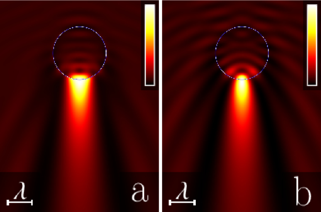
Figure 1: Near-field intensity distributions of the total wavefield in (a) the $x-z$ plane and (b) the $y-z$ plane for the LG beam with $m_{\mathrm{LG}}=0$, $f=0.05$ and $|\mathbf{R}_{d}|=0$. The parameters are: $R_{p}=\lambda$ is the scatterer radius and $n_{p}=1.3$ ($n_{\mathrm{m}}=1.0$) is the refractive index inside (outside) the particle.

IV.1 Photonic nanojets

For spherical particles illuminated by plane waves, formation of photonic nanojets and their structure was previously discussed in Refs. Lecler et al. (2005); Devilez et al. (2008); Geints et al. (2010). Plane waves can be regarded as Gaussian beams with $n=m_{\mathrm{LG}}=0$ and sufficiently small focusing parameter, $f\ll 1$, which is defined after Eq. (53) through the ratio of wavelength, $\lambda$, and the beam diameter at waist, $w_{0}$, $f=(2\pi)^{-1}\lambda/w_{0}$. This limiting case is illustrated in Fig. 1 which shows the near-field intensity distributions for the total light wavefield in both the $x-z$ and the $y-z$ planes computed at $m_{\mathrm{LG}}=0$ and $f=0.05$ for the spherical particle of the radius $R_{p}=\lambda$ with the refractive index $n_{p}=1.3$ (water) located in the air ($n_{\mathrm{m}}=1$).

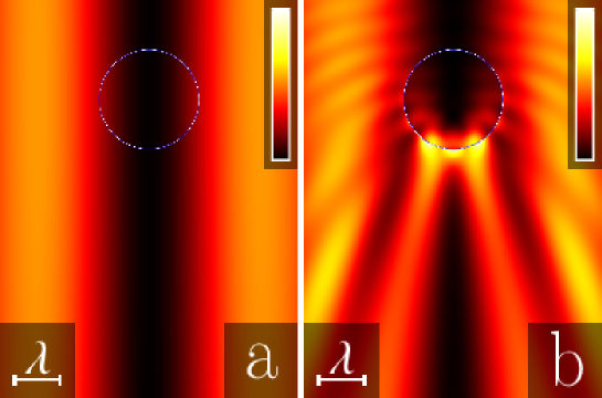
Figure 2: Near-field intensity distribution in the $x-z$ plane of (a) the incident wave beam and (b) the total wavefield for the LG beam with $m_{\mathrm{LG}}=1$, $f=0.05$ and $|\mathbf{R}_{d}|=0$. Other parameters are described in the caption of Fig. 1.

It can be seen that the distributions are characterized by the presence of elongated focusing zones formed near the shadow surface of the scatterer. The transverse size of these zones is smaller than the wavelength of incident light, whereas their longitudinal size in the direction of incidence which is along the $z$ axis from top to bottom is relatively large. Such a jetlike light structure is typical for the photonic nanojets. The characteristic length and width of nanojets along with the peak intensity are known to strongly depend on a number of factors such as the scatterer size $R_{p}$, the particle absorption coefficient and the optical contrast ratio $n_{p}/n_{\mathrm{m}}$. For microspheres, the results of a comprehensive numerical analysis including the case of shell particles are summarized in the recent paper Geints et al. (2010).

Effects of non-plane incident waves such as the laser beams on the structure of photonic nanojets are much less studied. Some theoretical results for tightly focused Gaussian beams are reported in Ref. Devilez et al. (2009) and the case of Bessel-Gauss beams was studied experimentally in Kim et al. (2011).

For the LG beams, we begin with the effects of the azimuthal mode number and describe what happens to the near-field structure shown in Fig. 1 when the azimuthal number takes the smallest non-zero value, $m_{\mathrm{LG}}=1$. The latter represents the simplest case of an optical vortex beam in which, owing to the presence of phase singularity, the intensity of incident light at the beam axis (the $z$ axis) vanishes (see Fig. 2(a)). From Fig. 2, it can be seen that, even though the bulk part of the scatterer is in the low intensity region surrounding the optical vortex, the scattering process is efficient enough to produce scattered waves that result in the formation of a pronounced jetlike photonic flux emerging from the particle shadow surface (see Fig. 2(b)).

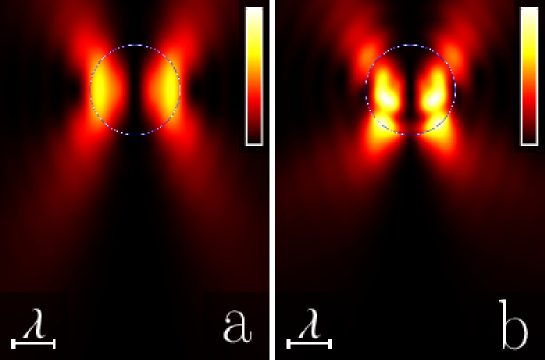
Figure 3: Near-field intensity distribution in the $x-z$ plane of (a) the incident wave beam and (b) the total wave field for the LG beam with $m_{\mathrm{LG}}=2$, $f=0.25$ and $|\mathbf{R}_{d}|=0$.

A comparison between Fig. 2(b) and Fig. 1(a) shows that the three-peak structure of the photonic jet formed at Mie scattering of the optical vortex LG beam with $m_{\mathrm{LG}}=1$ significantly differs from the well-known shape of the nanojet at $m_{\mathrm{LG}}=0$. Interestingly, similar to the case of Gaussian beams with $m_{\mathrm{LG}}=0$, the focusing zones at $m_{\mathrm{LG}}=1$ involve the beam axis where one of the light intensity peaks is located.

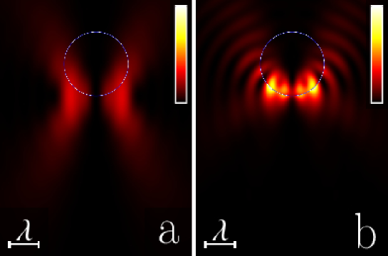
Figure 4: Near-field intensity distribution in the $x-z$ plane of (a) the incident wave beam and (b) the total wave field for the LG beam with $m_{\mathrm{LG}}=2$, $f=0.25$ and $\mathbf{R}_{d}=(0,0,\lambda)$.

The results for tightly focused LG beams with $m_{\mathrm{LG}}=2$ and $f=0.25$ are shown in Figs. 3 and 4. When the displacement vector, $\mathbf{R}_{d}$ defined in Eqs. (49) vanishes, the focal (waist) plane of the incident LG beam is $z=0$ and contains the center of the spherical scatterer (see Fig. 3(a)). Referring to Fig. 3, this is the case where, similar to the focal plane of the incident beam, the bulk part of the four-peak structure of the focusing zones is localized inside of the particles.

For $\mathbf{R}_{d}=(0,0,\lambda)$, the focal plane, $z=\lambda$, is tangential to the shadow part of the particle surface (see Fig. 4(a)). From Fig. 4(b), it is seen that, as opposed to the case with $|\mathbf{R}_{d}|=0$, the four peaks of light intensity now develop in the immediate vicinity of the scatterer surface.

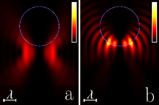
Figure 5: Near-field intensity distribution in the $x-z$ plane of (a) the incident wave beam and (b) the total wave field for the LG beam with $m_{\mathrm{LG}}=3$, $f=0.25$ and $\mathbf{R}_{d}=(0,0,\lambda)$.

What all the wavefields depicted in Figs. 2(b)- 4(b) have in common is that, by contrast to the incident optical vortex beams with $m_{\mathrm{LG}}=1$ and $m_{\mathrm{LG}}=2$, the light intensity on the incident beam axis (the $z$ axis) clearly differs from zero (see the neighborhood of the point $(0,0,\lambda)$). In other words, it is turned out that, in the near-field region, the optical vortex with $0<|m_{\mathrm{LG}}|\leq 2$ has been destroyed by Mie scattering. From Fig. 5 it is clear that this is no longer the case at $m_{\mathrm{LG}}=3$. This result will be explained in the subsequent section.

IV.2 Optical vortices in near-field region

In this section we consider optical vortices and their near-field structure. The optical vortices are known to represent phase singularities of complex-valued scalar waves which are zeros of the wavefield $\psi=|\psi|\exp(i\chi)$ where its phase $\chi$ is undefined. A phase singularity is characterized by the topological vortex charge $m_{V}$ defined as the closed loop contour integral of the wave phase $\chi$ modulo $2\pi$

$$m_{V}=\frac{1}{2\pi}\,\oint_{L}\mathrm{d}\chi,$$ (60)

where $L$ is the closed path around the singularity.

Optical vortices associated with the individual components of electric field will be of our primary concern. More specifically, we shall examine the optical vortex structure of the components $E_{z}$ and $E_{x}$ in the planes $z=z_{0}$ parallel to the $x-y$ plane. Since, in such planes, circles naturally play the role of closed loops, the starting point of our analysis is the electric field vector expressed as a function of the azimuthal angle $\phi$ in the following form:

$$\mathbf{E}=\sum_{\mu=-2}^{2}\mathbf{E}_{\mu}\exp[i(m_{\mathrm{LG}}+\mu)\phi]$$ (61)

$$\mathbf{E}_{\pm 2}\parallel\hat{\mathbf{x}}\mp i\hat{\mathbf{y}},\quad\mathbf{E}_{\pm 1}\parallel\hat{\mathbf{z}},\quad\mathbf{E}_{0}\perp\hat{\mathbf{z}}.$$ (62)

This formula gives the $\phi$ dependence of electric field expansion (17a) in which the coefficients are of the form given by Eq. (59). An immediate consequence of Eq. (61) is that $\mathbf{E}_{\mu}$ can be different from zero on the $z$ axis, $\mathbf{E}_{\mu}(0,0,z)\neq 0$, only if $m_{\mathrm{LG}}+\mu=0$.

From Eq. (62), at $|m_{\mathrm{LG}}|=1$, the electric field non-vanishing at the beam axis is linearly polarized along the $z$ axis, whereas it is circular polarized at $|m_{\mathrm{LG}}|=2$. The intensity distributions shown in Figs 1– 4 clearly indicate that, as opposed to the case with $m_{\mathrm{LG}}=3$ (see Fig. 5), the $z$ axis is not entirely in the dark region provided that $0\leq m_{\mathrm{LG}}<3$.

At $|m_{\mathrm{LG}}|\geq 3$ and $|\mu|\leq 2$, a sum $m_{\mathrm{LG}}+\mu$ cannot be equal to zero and the beam axis is always a nodal line for the components of electric field. For two-dimensional (2D) electric field distributions in planes normal to the $z$ axis, it implies that there is an optical vortex located at the origin.

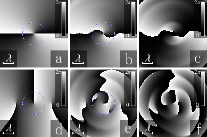
Figure 6: Near-field phase maps of the electric field components $E_{x}$ (a,b,c) and $E_{z}$ (d,e,f) in the planes $z=0$ (a,b,d,e) and $z=R_{p}$ (c,f) for the LG beam with $m_{\mathrm{LG}}=2$ and $f=0.1$. (a) [(d)] Phase map of the electric field component $E_{x}^{(\mathrm{LG})}$ [$E_{z}^{(\mathrm{LG})}$] of the incident wave beam in the $x-y$ plane ($z=0$). (b,c) [(e,f)] Phase maps for the electric field component $E_{x}$ [$E_{z}$] of the total light wavefield in the planes $z=0$ and $z=R_{p}$, respectively.

Now we turn back to the optical vortex structure for the components $E_{z}$ and $E_{x}$. The $\phi$ dependence of $E_{z}$ can be written in the following form:

$$\exp[-im_{\mathrm{LG}}\,\phi]E_{z}=\exp[-im_{\mathrm{LG}}\,\phi+i\chi_{z}]|E_{z}|=E_{+1}^{(z)}\exp[i\phi]+E_{-1}^{(z)}\exp[-i\phi]=$$

$$\exp[i\psi_{+}^{(z)}]\left\{|E_{+1}^{(z)}|\exp[i(\phi+\psi_{-}^{(z)})]+|E_{-1}^{(z)}|\exp[-i(\phi+\psi_{-}^{(z)})]\right\},$$ (63)

where $E_{\pm 1}^{(z)}=\bigl{(}{\mathbf{E}_{\pm 1}}\cdot{\hat{\mathbf{z}}}\bigr{)}$, $2\psi_{\pm}^{(z)}=\arg(E_{+1}^{(z)})\pm\arg(E_{-1}^{(z)})$ and $\chi_{z}$ is the phase of $E_{z}$.

In the complex plane formula (IV.2) describes an ellipse parametrized by the azimuthal angle $\phi$. It is centered at the origin with the major (minor) semiaxis of the length $E_{+}^{(z)}(R)$ ($|E_{-}^{(z)}(R)|$), where $E_{\pm}^{(z)}(R)=|E_{+1}^{(z)}(R)|\pm|E_{-1}^{(z)}(R)|$ $R$ is the radius of circle $C_{R}$ in the plane of observation, $z=z_{0}$. Then the closed loop contour integral of the wave phase $\chi_{z}$ is

$$m_{z}=\frac{1}{2\pi}\,\oint_{C_{R}}\mathrm{d}\chi_{z}=m_{\mathrm{LG}}+\mu_{z}(R),$$ (64a)

$$\mu_{z}(R)=\mathop{\rm sign}\nolimits(E_{-}^{(z)}(R))=\mathop{\rm sign}\nolimits(|E_{+1}^{(z)}(R)|-|E_{-1}^{(z)}(R)|).$$ (64b)

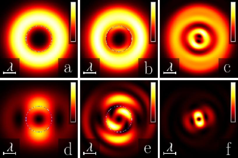
Figure 7: Near-field intensity maps of the electric field components $|E_{x}|^{2}$ (a,b,c) and $|E_{z}|^{2}$ (d,e,f) in the planes $z=0$ (a,b,d,e) and $z=R_{p}$ (c,f) for the LG beam with $m_{\mathrm{LG}}=2$ and $f=0.1$. (a) [(d)] Intensity distribution for the $x$ [$z$] component, $|E_{x}^{(\mathrm{LG})}|^{2}$ [$|E_{z}^{(\mathrm{LG})}|^{2}$], of the incident wave beam in the $x-y$ plane ($z=0$). (b,c) [(e,f)] Intensity distributions for the $x$ [$z$] component of electric field of the total light wavefield in the planes $z=0$ and $z=R_{p}$, respectively.

From Eq. (64) the net topological charge of vortices encircled by $C_{R}$ can be either $m_{\mathrm{LG}}+1$ or $m_{\mathrm{LG}}-1$. At $|E_{+1}^{(z)}(R)|=|E_{-1}^{(z)}(R)|$, $\mu_{z}(R)$ is undefined. This is the special case when $|E_{z}|=0$ at $\cos(\phi+\psi_{-}^{(z)})=0$ and the circle contains a pair of symmetrically located vortices. Each of these vortices carries the charge of the magnitude equal to unity. Generally, the vortices are of the same sign which is determined by the change of $\mu_{z}(R)$ as the radius $R$ passes the critical value. When $\mu_{z}(R)$ changes from $+1$ ($-1$) to $-1$ ($+1$) two vortices of the charge $-1$ ($+1$) intersect the boundary and move into the interior part of the circle.

The near field phase maps for $\chi_{z}$ are presented in Figs. 6(d)–(f). Figure 6(d) shows the 2D map for the incident optical vortex LG beam with $m_{\mathrm{LG}}=2$ in the focal plane $z=0$. The corresponding intensity map is depicted in Fig. 7(d). It is seen that there is a vortex of the charge $m_{\mathrm{LG}}-1=1$ at the center, so that, at sufficiently small $R$, $m_{z}=1$ and $\mu_{z}=-1$. In addition, there is a pair of the symmetrically arranged vortices of the charge $+1$ outside the particle. So, when the radius $R$ is large enough for the circle to enclose the three vortices, the total charge is $m_{z}=m_{\mathrm{LG}}+1=3$ and $\mu_{z}=1$.

For the total wavefield at $z=0$, the phase and intensity maps are given in Fig. 6(e) and Fig. 7(e), respectively. It can be seen that the vortex pattern is complicated by interference between the incident and the scattered waves. Referring to Fig. 6(e), there are two additional pairs of vortices whose charges are opposite in sign. The positively charged vortices (the charge is $+1$) are located inside the particle, whereas the negatively charged ones (the charge is $-1$) are formed at the surface of the particle. Similar structure is discernible from Figs. 6(f) and 7(f) representing the results for the plane tangent to the particle surface $z=R_{p}$.

The case of the $x$ component of the electric field, $E_{x}$, can be analyzed along similar lines. From Eq. (61), we deduce the $\phi$ dependence of $E_{x}$ in the form:

$$\exp[-im_{\mathrm{LG}}\,\phi+i\chi_{x}]|E_{x}|-E_{0}^{(x)}=E_{+2}^{(x)}\exp[2i\phi]+E_{-2}^{(x)}\exp[-2i\phi]=$$

$$\exp[i\psi_{+}^{(x)}]\left\{|E_{+2}^{(x)}|\exp[i(2\phi+\psi_{-}^{(x)})]+|E_{-2}^{(x)}|\exp[-i(2\phi+\psi_{-}^{(x)})]\right\},$$ (65)

where $E_{\pm 2,\,0}^{(x)}=\bigl{(}{\mathbf{E}_{\pm 2,\,0}}\cdot{\hat{\mathbf{x}}}\bigr{)}$, $2\psi_{\pm}^{(x)}=\arg(E_{+2}^{(x)})\pm\arg(E_{-2}^{(x)})$ and $\chi_{x}$ is the phase of $E_{x}$. The center of the ellipse described by Eq. (IV.2) is generally displaced from the origin and is determined by $E_{0}^{(x)}$. The length of its major (minor) semiaxis is $E_{+}^{(x)}(R)$ ($|E_{-}^{(x)}(R)|$), where $E_{\pm}^{(x)}(R)=|E_{+2}^{(x)}(R)|\pm|E_{-2}^{(x)}(R)|$.

The closed loop contour integral of the wave phase $\chi_{x}$ is

$$m_{x}=\frac{1}{2\pi}\,\oint_{C_{R}}\mathrm{d}\chi_{x}=m_{\mathrm{LG}}+\mu_{x}(R),\quad\mu_{x}(R)\in\{-2,0,2\}.$$ (66)

When the origin is enclosed by the ellipse (IV.2), similar to Eq. (64b), we have the relation

$$\mu_{x}(R)=2\mathop{\rm sign}\nolimits(E_{-}^{(x)}(R))=2\mathop{\rm sign}\nolimits(|E_{+2}^{(x)}(R)|-|E_{-2}^{(x)}(R)|).$$ (67)

In the opposite case where the origin is outside the area encircled by the ellipse, $\mu_{x}(R)$ is zero. The latter is the case for the phase maps representing the 2D distributions of $\chi_{x}$ in the $x-y$ plane (see Figs. 6(a)–(b)). As is evident from Figs. 6(a)–(b) (see also the intensity maps in Figs. 7(a)–(b)), in these distributions, the only vortex is positioned at the center and possesses the charge $m_{x}=m_{\mathrm{LG}}=2$.

For the origin located on the ellipse, we generally have the circle $C_{R}$ containing a pair of symmetrically arranged and identically charged vortices each with the charge magnitude equal to unity. Note that, by contrast to the case of $E_{z}$ where the origin is placed at the center of the ellipse (IV.2), intersection of $C_{R}$ and the vortices generally occurs at non-vanishing $E_{-}^{(x)}$, $E_{-}^{(x)}\neq 0$, when the ellipse (IV.2) is not degenerated into the interval.

In Fig. 6(c), we show what happen to the above discussed central vortex in the tangent plane of the particle surface, $z=R_{p}$. From the phase and intensity maps (see Figs. 6(c) and 7(c)), the central vortex has been destroyed and is replaced by a pair of positively charged and symmetrically arranged vortices. In this vortex pattern, $\mu_{x}(R)=-2$ at small $R$, whereas $\mu_{x}(R)$ becomes zero when the vortices are encircled by $C_{R}$. For the ellipse (IV.2), it means that the origin, which is initially encompassed by the ellipse with $E_{-}^{(x)}<0$, intersects the ellipse and moves outward the area bounded by the ellipse as $R$ increases.

V Conclusions

In this paper, we have used a modified $T$–matrix approach Kiselev et al. (2002a) to study the light scattering problem for optically isotropic spherical scatterers illuminated with LG beams that represent optical vortex laser beams. In our approach, such beams are described in terms of the far-field angular distribution (38) using the remodelling procedure in which the far-field matching method is combined with the results for nonparaxial propagation of LG beams (see Eq. (55)).

The analytical results are employed to perform numerical analysis of the optical field in the near-field region. In order to examine the effects of incident beam spatial structure on the light wavefield near the scatterer, we have computed a number of the 2D near-field intensity and phase distributions for purely azimuthal LG beams. In this case, a LG beam possesses the vanishing radial mode number and carries the optical vortex with the topological charge characterized by the azimuthal number $m_{\mathrm{LG}}$.

The 2D near-field intensity distributions computed for the plane-wave limiting case in which the incident wave is a Gaussian beam ($m_{\mathrm{LG}}=0$) with small focusing parameter $f$ ($2\pi f=\lambda/w_{0}<1$) reveal the well-known structure of photonic nanojets (see Fig. 1). Figures 2– 5 represent the results for the LG beams with $1\leq m_{\mathrm{LG}}\leq 3$ and illustrate the following effects:

1. a jetlike photonic flux emerging from the particle shadow surface can be formed even if the bulk part of the scatterer is in the low intensity region (see Fig. 2(b));

2. the morphology of photonic jets formed at $m_{\mathrm{LG}}\neq 0$ significantly differs from the well-known shape of nanojet at $m_{\mathrm{LG}}=0$ (see Figs. 3– 5);

3. by contrast to the case with $m_{\mathrm{LG}}=3$, at $|m_{\mathrm{LG}}|<3$, the intensity of scattered wavefield does not vanish on the beam axis so that, in the near-feld region, lght scattering has a destructive effect on the optical vortex (see Figs. 2– 4).

Our analysis of optical vortices associated with the electric field components is based on general formula (61) giving the electric field vector expressed as a function of the azimuthal angle $\phi$. Using analytical expressions (IV.2) and (IV.2), we have described the geometry of optical vortices for the components $E_{z}$ and $E_{x}$ in the planes $z=z_{0}$ normal to the beam axis (the $z$ axis).

It was found that, except for the central vortex, the topological charge of off-center vortices generally equals unity in magnitude. They are organized into pairs of symmetrically arranged and equally charged vortices. These pairs lie on concentric circles and their vortex charge alternate in sign with the circle radius.

The phase maps of $E_{x}$ shown in Figs. 6(a)-(c) (the corresponding square amplitude distributions are presented in Figs. 7(a)-(c)) are computed for the LG beam with $m_{\mathrm{LG}}=2$. It turned out that the central vortex of the charge equal to the azimuthal number $m_{\mathrm{LG}}=2$ is the only vortex in the $x-y$ plane ($z=0$) for both the incident beam (see Fig. 6(a)) and the total wavefield (see Fig. 6(b)). At $z=R_{d}$, this vortex breaks down into a pair of vortices each of the unity charge $m_{V}=1$ (see Fig. 6(c)).

By contrast to the case of $E_{x}$, Eq. (IV.2) implies that the $z$ axis is a nodal line for the $z$ component of the electric field $E_{z}$ and the central vortex is structurally stable at $m_{\mathrm{LG}}=2$ (see Figs. 6(d)-(f)). A comparison between the phase maps for the incident beam (see Fig. 6(d)) and for the total light field (see Fig. 6(e)) shows that, in the $x-y$ plane, interference between the incident and the scattered waves produces two additional pairs of vortices.

In conclusion, an important consequence of formula (61) is that, at sufficiently large azimuthal numbers, $|m_{\mathrm{LG}}|\geq 3$, light scattering of LG beams takes place without destroying the optical vortex located on the beam axis.

References

• Mie (1908) G. Mie, Ann. Phys. (Leipzig) 25, 377 (1908).
• Newton (1982) R. G. Newton, Scattering Theory of Waves and Particles, 2nd ed. (Springer, Heidelberg, 1982).
• Bohren and Huffman (1983) C. F. Bohren and D. R. Huffman, Absorption and Scattering of Light by Small Particles (Wiley-Interscience, New York, 1983).
• Tsang et al. (2000) L. Tsang, J. A. Kong,  and K.-H. Ding, Scattering of Electromagnetic Waves. Theories and Applications, Wiley Series in Remote Sensing, Vol. 1 (Wiley–Interscience Pub, NY, 2000) p. 426.
• Mishchenko et al. (2004) M. I. Mishchenko, L. D. Travis,  and A. A. Lacis, Scattering, Absorption and Emission of Light by Small Particles (Cambridge University Press, NY, 2004) p. 448.
• Doicu et al. (2006) A. Doicu, T. Wriedt,  and Y. A. Eremin, Light Scattering by Systems of Particles. Null-Field Method with Discrete Sources: Theory and Programs, Springer Series in Optical Sciences (Springer, Berlin, 2006) p. 322.
• Gouesbet and Gréhan (2011) G. Gouesbet and G. Gréhan, Generalized Lorenz–Mie theories (Springer, Berlin, 2011) p. 310.
• Mishchenko et al. (1996) M. I. Mishchenko, L. D. Travis,  and D. W. Mackowski, J. of Quant. Spectr. & Radiat. Transf. 55, 535 (1996).
• Mishchenko et al. (2000) M. I. Mishchenko, J. W. Hovenier,  and L. D. Travis, eds., Light Scattering by Nonspherical Particles: Theory, Measurements and Applications (Academic Press, New York, 2000).
• Roth and Digman (1973) J. Roth and M. J. Digman, J. Opt. Soc. Am. 63, 308 (1973).
• Lange and Aragon (1990) B. Lange and S. R. Aragon, J. Chem. Phys. 92, 4643 (1990).
• Hahn and Aragon (1994) D. K. Hahn and S. R. Aragon, J. Chem. Phys. 101, 8409 (1994).
• Karacali et al. (1997) H. Karacali, S. M. Risser,  and K. F. Ferris, Phys. Rev. E 56, 4286 (1997).
• Kiselev et al. (2000) A. D. Kiselev, V. Y. Reshetnyak,  and T. J. Sluckin, Opt. Spectrosc. 89, 907 (2000).
• Kiselev et al. (2002a) A. D. Kiselev, V. Y. Reshetnyak,  and T. J. Sluckin, Phys. Rev. E 65, 056609 (2002a).
• Geng et al. (2004) Y.-L. Geng, X.-B. Wu, L.-W. Li,  and B.-R. Guan, Phys. Rev. E 70, 056609 (2004).
• Novitsky and Barkovsky (2008) A. Novitsky and L. Barkovsky, Phys. Rev. A 77, 033849 (2008).
• Qiu et al. (2010) C. Qiu, L. Gao, J. D. Joannopoulos,  and M. Soljačić, Laser & Photon. Rev. 4, 268 (2010).
• Grehan et al. (1986) G. Grehan, B. Maheu,  and G. Gouesbet, Appl. Opt. 25, 3539 (1986).
• Gouesbet et al. (1988a) G. Gouesbet, B. Maheu,  and G. Gréhan, J. Opt. Soc. Am. A 5, 1427 (1988a).
• Barton et al. (1988) J. P. Barton, D. R. Alexander,  and S. A. Schaub, J. Appl. Phys. 64, 1632 (1988).
• Barton et al. (1989) J. P. Barton, D. R. Alexander,  and S. A. Schaub, J. Appl. Phys. 65, 4594 (1989).
• Schaub et al. (1992) S. A. Schaub, D. R. Alexander,  and J. P. Barton, J. Opt. Soc. Am. A 9, 316 (1992).
• Lock and Gouesbet (2009) J. A. Lock and G. Gouesbet, J. of Quant. Spectr. & Radiat. Transf. 110, 800 (2009).
• Gouesbet et al. (1988b) G. Gouesbet, G. Grehan,  and B. Maheu, Appl. Opt. 27, 4874 (1988b).
• Gouesbet et al. (2011) G. Gouesbet, J. A. Lock,  and G. Gréhan, J. of Quant. Spectr. & Radiat. Transf. 112, 1 (2011).
• Lax et al. (1975) M. Lax, W. H. Louisell,  and W. B. McKnight, Phys. Rev. A 11, 1365 (1975).
• Davis (1979) L. W. Davis, Phys. Rev. A 19, 1177 (1979).
• Nieminen et al. (2003) T. A. Nieminen, H. Rubinsztein-Dunlop,  and N. R. Heckenberg, J. of Quant. Spectr. & Radiat. Transf. 79-80, 1005 (2003).
• Bareil and Sheng (2013) P. B. Bareil and Y. Sheng, J. Opt. Soc. Am. A 30, 1 (2013).
• Hoang et al. (2012) T. X. Hoang, X. Chen,  and C. J. R. Sheppard, J. Opt. Soc. Am. A 29, 32 (2012).
• Barnett and Allen (1994) S. M. Barnett and L. Allen, Opt. Commun. 110, 670 (1994).
• Duan et al. (2005) K. Duan, B. Wang,  and B. Lü, J. Opt. Soc. Am. A 22, 1976 (2005).
• Van De Nes et al. (2006) A. S. Van De Nes, S. F. Pereira,  and J. J. M. Braat, Journal of Modern Optics 53, 677 (2006).
• Zhou (2006) G. Zhou, Opt. Lett. 31, 2616 (2006).
• Zhou (2008) G. Zhou, Optics & Laser Technology 40, 930 (2008).
• van de Ness and Török (2007) A. S. van de Ness and P. Török, Opt. Express 15, 6417 (2007).
• Jiang et al. (2012) Y. Jiang, Y. Shao, X. Qu, J. Ou,  and H. Hua, J. Opt. 14, 125709 (2012).
• Allen et al. (2003) L. Allen, S. M. Barnett,  and M. J. Padgett, eds., Optical Angular Momentum (Taylor & Francis, London, 2003).
• Desyatnikov et al. (2005) A. S. Desyatnikov, Y. S. Kivshar,  and L. Torner, in Progress in Optics, Vol. 47, edited by E. Wolf (North-Holland, Amsterdam, 2005) Chap. 5, pp. 291–391.
• Andrews (2008) D. L. Andrews, ed., Structured Light and Its Applications: An Introduction to Phase-Structured Beams and Nanoscale Optical Forces (Academic Press, Amsterdam, 2008) p. 342.
• Simpson and Hanna (2009) S. H. Simpson and S. Hanna, J. Opt. Soc. Am. A 26, 173 (2009).
• Simpson and Hanna (2010) S. H. Simpson and S. Hanna, J. Opt. Soc. Am. A 27, 2061 (2010).
• Heifetz et al. (2009) A. Heifetz, S.-C. Kong, A. V. Sahakian, A. Taflove,  and V. Backman, J. Comput. Theor. Nanosci. 12, 1214 (2009).
• Chen et al. (2004) Z. Chen, A. Taflove,  and V. Backman, Opt. Express 12, 1214 (2004).
• Li et al. (2005) X. Li, Z. Chen, A. Taflove,  and V. Backman, Opt. Express 13, 526 (2005).
• Lecler et al. (2005) S. Lecler, Y. Takakura,  and P. Meyrueis, Opt. Lett. 30, 2641 (2005).
• Devilez et al. (2008) A. Devilez, B. Stout, N. Bonod,  and E. Popov, Opt. Express 16, 14200 (2008).
• Geints et al. (2010) Y. E. Geints, A. A. Zemlyanov,  and E. K. Panina, Opt. Commun. 283, 4775 (2010).
• Ding et al. (2010) H. Ding, L. Dai,  and C. Yan, Chin. Opt. Lett. 8, 706 (2010).
• Geints et al. (2012) Y. E. Geints, A. A. Zemlyanov,  and E. K. Panina, J. Opt. Soc. Am. B 29, 758 (2012).
• Guo et al. (2013) H. Guo, Y. Han, X. Weng, Y. Zhao, G. Sui, Y. Wang,  and S. Zhuang, Opt. Express 16, 6930 (2013).
• Biedenharn and Louck (1981) L. C. Biedenharn and J. D. Louck, Angular Momentum in Quantum Physics: Theory and Application, Encyclopedia of Mathematics and its Applications, Vol. 8 (Addison–Wesley, Reading, Massachusetts, 1981) p. 717.
• Varshalovich et al. (1988) D. A. Varshalovich, A. N. Moskalev,  and V. K. Khersonskii, Quantum theory of angular momentum: Irreducible tensors, spherical harmonics, vector coupling coefficients, 3nj symbols (World Scientific Publishing Co., Singapore, 1988) p. 514.
• Jackson (1999) J. D. Jackson, Classical Electrodynamics, 3rd ed. (Wiley, New York, 1999).
• Abramowitz and Stegun (1972) M. Abramowitz and I. A. Stegun, eds., Handbook of Mathematical Functions (Dover, New York, 1972).
• Sarkar and Halas (1997) D. Sarkar and N. J. Halas, Phys. Rev. E 56, 1102 (1997).
• Kiselev et al. (2002b) A. D. Kiselev, V. Y. Reshetnyak,  and T. J. Sluckin, Mol. Cryst. Liq. Cryst. 375, 373 (2002b).
• Ishimaru (1978) A. Ishimaru, Wave Propagation and Scattering in Random Media (Academic Press, New York, 1978).
• Gradshteyn and Ryzhik (1980) I. S. Gradshteyn and I. M. Ryzhik, Table of Integrals, Series, and Products (Academic, New York, 1980).
• Nienhuis and Allen (1993) G. Nienhuis and L. Allen, Phys. Rev. A 48, 656 (1993).
• Enderlein and Pampaloni (2004) J. Enderlein and F. Pampaloni, J. Opt. Soc. Am. A 21, 1553 (2004).
• Sherman et al. (1976) G. C. Sherman, J. J. Stamnes,  and E. Lalor, J. Math. Phys. 17, 760 (1976).
• Rury and Freeling (2012) A. S. Rury and R. Freeling, Phys. Rev. A 86, 053830 (2012).
• Devilez et al. (2009) A. Devilez, N. Bonod, J. Wegner, D. Gérard, B. Stout, H. Rigneault,  and E. Popov, Opt. Express 17, 2089 (2009).
• Kim et al. (2011) M.-S. Kim, T. Scharf, S. Mühlig, C. Rockstuhl,  and H. P. Herzig, Opt. Express 19, 10206 (2011).