Stable Exact Cosmological Solutions in Induced Gravity Models

Abstract

We study dynamics of induced gravity cosmological models with sixth degree potential, that have found using the superpotential method. The important property of these models are existence of exact cosmological solutions that tend to fixed points. The stability of these cosmological solutions have been obtained. In particular, we find conditions under which solutions with a non-monotonic Hubble parameter that tend to a fixed point are attractors.

1 Introduction

A large number of observational data [1, 2, 3, 4, 5, 6, 7, 8] supports that the post-inflationary Universe is nearly homogeneous and isotropic and that the expansion of the Universe is accelerating. It was also shown that the Universe is spatially flat at large distances.

There are two possible ways of describing the accelerating expansion of the Universe. The assumption that General Relativity is the correct theory of gravity leads to the conclusion that there exists and currently dominates a smoothly distributed, slowly varying cosmic fluid with negative pressure, so-called dark energy [9, 10, 11]. The simplest way to describe the dark energy is to add the cosmological constant to the Einstein–Hilbert action. Another popular variant is to consider models with scalar fields [10, 11, 12]. There are a few reason to consider cosmological models with scalar fields. First of all there is no doubt that the evolution of the Universe can be described by the spatially flat Friedmann–Lemaître–Robertson–Walker (FLRW) background and cosmological perturbations. Models with scalar fields are very useful to describe such a type of the evolution. That is why scalar fields play an essential role in modern cosmology, in particular, in the current description of the evolution of the Universe at the early epoch [13, 14, 15, 16, 17, 18].

To specify the cosmic fluid one typically uses a phenomenological relation $p=w\varrho$ between the pressure (Lagrangian density) $p$ and the energy density $\varrho$ of this fluid. If a model includes only one cosmic fluid then in the FLRW metric the equation of state parameter $w$ and the Hubble parameter $H$ are connected as follows:

$$w={}-1-\frac{2\dot{H}}{3H^{2}},$$

where differentiation with respect to the cosmic time $t$ is denoted by a dot.

The cosmological constant corresponds to a constant $H$ (de Sitter Universe). The standard way to obtain an evolving Hubble parameter is to add scalar fields to a cosmological model. It has been demonstrated that dark energy with an evolving equation of state parameter provides a compelling alternative to a cosmological constant if data are analysed in a prior-free manner and the weak energy condition is not imposed by hand [19]. For the model with minimally coupled scalar with the standard kinetic term we get $w>-1$ and the Hubble parameter is a monotonically decreasing function. To get non-monotonic behaviour of the Hubble parameter one needs either to add a phantom scalar field and get a quintom model [20, 21, 22, 23, 24], or consider a scalar field with the second-derivative Lagrangian (see [25] as a review). Note that the dark energy equation of state parameter can be less than $-1$, since this possibility is not excluded by astrophysical data [19, 26]. At the same time the cosmological models with $w<-1$ violate the null energy condition (NEC), this violation is generally related to the phantom fields appearing. The standard quantization of these models leads to instability, which is physically unacceptable. Examples of cosmological models with nonstandard scalar fields that admit solutions violating the NEC and having no obvious pathologies are presented in [25].

Note that consideration of models with phantom scalar fields can be motivated by the string field theory [27, 28, 29, 21]. The theory with $w<-1$ can be interpreted as an approximation in the framework of the fundamental theory. Because the fundamental theory must be stable and must admit quantization, this instability can be considered an artefact of the approximation. In the FLRW metric the NEC violating models can have classically stable solutions cosmology. In particular, there are classically stable solutions for self-interacting ghost models with minimal coupling to gravity. Moreover, there exists an attractor behavior in a class of the phantom cosmological models [30, 31, 32].

Alternative way to describe the dark energy is to modify the theory of gravity [33, 34, 35, 36]. Some of popular modified gravity models, for example, ${\cal F}(R)$ gravity models, can then be mapped into general relativity models with additional scalar fields by a suitable conformal transformation of the metric (see, e.g., [35, 36, 37]). Another example is a class of nonlocally modified gravity models which were proposed to explain the current phase of cosmic acceleration without dark energy [38] (see also [39, 40, 41, 42] and the review [43]). These models do not assume the existence of a new dimensional parameter in the action and include a function $f(\Box^{-1}R)$, with $\Box$ the d’Alembertian operator. These nonlocal models have a local scalar-tensor formulation that has been proposed in [44], developed and used in [45, 46, 47, 48, 49].

Predictions of simplest inflationary models are in disagreement with the Planck2013 results [8]. At the same time many of these inflationary scenarios can be improved by adding a tiny non-minimal coupling of the inflaton field to gravity [50, 51]. In the last years, the Higgs-driven inflation that includes non-minimal coupling between the Higgs boson and gravity has attracted a lot of attention [52, 53, 54, 55, 56, 57].

The models with the Ricci scalar multiplied by a function of the scalar field are being intensively studied in cosmology [58, 59, 60, 61, 62, 63, 64, 65, 66, 67, 68, 69, 70] (see also [33, 35, 36] and references therein). Generally these models are described by the following action:

$$S=\int d^{4}x\sqrt{-g}\left[U(\phi)R-\frac{1}{2}g^{\mu\nu}\phi_{,\mu}\phi_{,\nu}-V(\phi)\right],$$ (1)

where $U(\phi)$ and $V(\phi)$ are differentiable functions of the scalar field $\phi$, $g$ is the determinant of the metric tensor $g_{\mu\nu}$ and the signature $(-,+,+,+)$ is used.

The reconstruction procedure for the induced gravity models ($U(\phi)=\xi\phi^{2}$, where $\xi$ is a constant) has been proposed in [66]. In such a case it has been shown that one can linearize all the differential equations that should be solved in the reconstruction procedure to get the potential corresponding to a given cosmological evolution. This property allows one to obtain the explicit forms of potentials reproducing the dynamics of a spatially flat FLRW universe, driven by barotropic perfect fluids, by a Chaplygin gas and by a modified Chaplygin gas [66].

In [69] another reconstruction procedure for the models described by action (1) has been considered. Such a method is similar to the Hamilton–Jacobi method (also known as the superpotential method or the first-order formalism) and is applied to cosmological models with scalar fields [71, 28, 72, 21, 73, 74, 75, 76]. Note that similar method is used for the reconstruction procedure in brane models [77, 78] and in holographic models [79, 80]. The key point in this method is that the Hubble parameter is considered as a function of the scalar field $\phi$. These two methods described above supplement each other and together allow one to construct different cosmological models with some required properties.

In this paper we study the stability of solutions in the FLRW metric, considering isotropic and homogenous fluctuations only. In other word, we assume that not only background solution, but also perturbations are homogeneous and isotropic. We analyse the stability with respect to small fluctuations of the initial data.

In [69], induced gravity models with the sixth degree polynomial potentials and physically interesting behaviors of the Hubble parameter have been obtained. To get these models the superpotential method has been used, because the explicit form of the Hubble parameter $H(t)$ is too complicated to be guessed. In particular, solutions with non-monotonic behaviors of the Hubble parameter have been obtained. In this paper we consider the stability of these solutions.

The stability of a continuous solution tending to a fixed point (kink or lump like solutions) implies the stability of this fixed point. This fixed point is a de Sitter solution if the corresponding Hubble parameter is not equal to zero. De Sitter solutions which are attractors of the system describing the cosmological dynamics of non-minimally coupled scalar field have been investigated in [67]. In this paper we use the Lyapunov theorem [81, 82] and find conditions under which the fixed point and the corresponding kink (or lump) solution are stable. In these cases the necessary condition of exact solution’s stability is boundedness of the first corrections for positive time semiaxis. In particular we find conditions under which solutions this nonmonotonic behaviour of the Hubble parameter are stable.

The paper is organized as follows. In Section 2, we review the basic equations for a induced gravity model and remind the algorithm of the superpotential reconstruction procedure. In Section 3 we consider induced gravity cosmological models. In Section 4, we find solutions and potentials with a Hubble parameter that evolves toward a constant value at late times. In Section 5 we obtain the stability conditions. In Section 6, we analyse the stability of the kink-type solutions. Finally Section 7 is devoted to the conclusions.

2 Cosmological models with non-minimally coupled scalar fields

Let us consider the spatially flat FLRW universe with the interval

$$ds^{2}={}-dt^{2}+a^{2}(t)\left(dx_{1}^{2}+dx_{2}^{2}+dx_{3}^{2}\right).$$

The Friedmann equations derived by variation of action (1) have the following form [66, 69]:

$$6UH^{2}+6\dot{U}H=\frac{1}{2}\dot{\phi}^{2}+V,$$ (2)

$$2U\left(2\dot{H}+3H^{2}\right)+4\dot{U}H+2\ddot{U}+\frac{1}{2}\dot{\phi}^{2}-V=0,$$ (3)

where the Hubble parameter is the logarithmic derivative of the scale factor: $H=\dot{a}/a$. The variation of action (1) with respect to $\phi$ gives

$$\ddot{\phi}+3H\dot{\phi}+V^{\prime}=6\left(\dot{H}+2H^{2}\right)U^{\prime}\,,$$ (4)

where the prime indicates the derivative with respect to the scalar field $\phi$. Combining Eqs. (2) and (3) we obtain

$$4U\dot{H}-2\dot{U}H+2\ddot{U}+\dot{\phi}^{2}=0.$$ (5)

From Eqs. (2)–(5), one can get the following system of the first order equations [68]:

$$\begin{split}\dot{\phi}&=\psi,\\ \dot{\psi}&={}-3H\psi-\frac{\left[(6U^{\prime\prime}+1)\psi^{2}-4V\right]U^{\prime}+2UV^{\prime}}{2\left(3{U^{\prime}}^{2}+U\right)},\\ \dot{H}&={}-\frac{2U^{\prime\prime}+1}{4\left(3{U^{\prime}}^{2}+U\right)}\psi^{2}+\frac{2U^{\prime}}{{3{U^{\prime}}^{2}+U}}H\psi-\frac{6{U^{\prime}}^{2}}{3{U^{\prime}}^{2}+U}H^{2}+\frac{U^{\prime}V^{\prime}}{2\left(3{U^{\prime}}^{2}+U\right)}\,.\end{split}$$ (6)

Note that Eq. (2) is not a consequence of system (6). On the other hand, if Eq. (2) is satisfied in the initial moment of time, then from system (6) it follows that Eq. (2) is satisfied at any moment of time. In other words, system (6) is equivalent to the initial system of equations (2)–(4) if and only if we choose such initial data that Eq. (2) is satisfied.

Let $H=Y(\phi)$ and the function ${\cal F}(\phi)$ is defined as follows

$$\dot{\phi}={\cal F}(\phi).$$ (7)

Substituting $\dot{\phi}$ and $\ddot{\phi}={\cal F}^{\prime}{\cal F}$ into Eq. (5), one obtains the following equation [69]:

$$4UY^{\prime}+2({\cal F}^{\prime}-Y)U^{\prime}+\left(2U^{\prime\prime}+1\right){\cal F}=0.$$ (8)

Equation (8) contains three functions. If two of them are given, then the third one can be found as the solution of a linear differential equation. Let us note that Eq. (8) is a first order differential equation for both $Y$ and $F$.

The potential $V(\phi)$ can be obtained from (2):

$$V(\phi)=6UY^{2}+6U^{\prime}{\cal F}Y-\frac{1}{2}{\cal F}^{2}.$$ (9)

To find the function $\phi(t)$ and, hence, $H(t)=Y(\phi(t))$ we integrate Eq. (7).

Let system (6) has a constant solution (fixed point): $(\phi_{f},\psi_{f},H_{f})$. For such a solution $\psi_{f}=0$ and

$$V(\phi_{f})=6U(\phi_{f})H_{f}^{2},\qquad V^{\prime}(\phi_{f})=2\frac{U^{\prime}(\phi_{f})}{U(\phi_{f})}V(\phi_{f}).$$ (10)

In terms of functions ${\cal F}$ and $Y$ we get the following conditions for fixed point:

$${\cal F}(\phi_{f})=0,\qquad V(\phi_{f})=6U(\phi_{f})Y(\phi_{f})^{2},\qquad V^{\prime}(\phi_{f})=12U^{\prime}(\phi_{f})Y(\phi_{f})^{2}.$$ (11)

3 Induced gravity cosmological models

In this paper, we are interested in the induced gravity models [59, 66] with

$$U(\phi)=\frac{\xi}{2}\phi^{2}\,,$$ (12)

where $\xi$ is the non-minimal coupling constant.

Equations (2)–(4) for such choice of the function $U(\phi)$ look as follows:

$$H^{2}=\frac{V}{3\xi\phi^{2}}+\frac{1}{6\xi}\left(\frac{\dot{\phi}}{\phi}\right)^{2}-2H\frac{\dot{\phi}}{\phi},$$ (13)

$$3H^{2}+2\dot{H}={}-2\frac{\ddot{\phi}}{\phi}-4H\frac{\dot{\phi}}{\phi}-\frac{4\xi+1}{2\xi}\left(\frac{\dot{\phi}}{\phi}\right)^{2}+\frac{V}{\xi\phi^{2}},$$ (14)

$$\ddot{\phi}+3H\dot{\phi}+V^{\prime}-6\xi\phi\left(2H^{2}+\dot{H}\right)=0,$$ (15)

and system (6) has the following form:

$$\begin{split}\dot{\phi}&=\psi,\\ \dot{\psi}&={}-3H\psi-\frac{\psi^{2}}{\phi}+\frac{1}{(1+6\xi)\phi}[4V(\phi)-\phi V^{\prime}(\phi)],\\ \dot{H}&=\frac{4H\psi}{(1+6\xi)\phi}+\frac{V^{\prime}(\phi)}{(1+6\xi)\phi}-\frac{12\xi}{1+6\xi}H^{2}-\frac{1+2\xi}{2\xi(1+6\xi)}\left(\frac{\psi}{\phi}\right)^{2}.\end{split}$$ (16)

It has been shown in [68] that at $\xi=-1/6$ nontrivial solutions in the FLRW metric exist for the potential $V=V_{0}\phi^{4}$ only. By this reason, we assume that $\xi\neq-1/6$.

For induced gravity models we get from equation (8) that

$${\cal F}(\phi)=\phi^{-1-1/(2\xi)}\left[B_{1}-\int\phi^{(2\xi+1)/(2\xi)}\left(Y^{\prime}\phi-Y\right)d\!\phi\right],$$ (17)

where $B_{1}$ is an arbitrary constant.

4 Different behavior of the Hubble Parameter

Let $Y(\phi)$ is a generic quadratic polynomial

$$Y(\phi)=C_{0}+C_{1}\phi+C_{2}\phi^{2},$$ (18)

where $C_{0}$, $C_{1}$, and $C_{2}$ are arbitrary constants, but $C_{2}\neq 0$. From (17) we obtain

$${\cal F}(\phi)=\frac{2\left((8\xi+1)C_{0}-(4\xi+1)C_{2}\phi^{2}\right)\xi\phi}{(4\xi+1)(8\xi+1)}+B\phi^{-(1+2\xi)/(2\xi)},$$ (19)

where $B$ is an arbitrary constant. Note that the function ${\cal F}(\phi)$ does not depend on $C_{1}$. We assume that $\xi\neq-1/4$ and $\xi\neq-1/8$. When $B=0$, the function ${\cal F}(\phi)$ is a cubic polynomial and the general solution for Eq. (7) can be written in terms of elementary functions.

For $C_{0}\neq 0$ we obtain

$$\phi_{\pm}(t)=\pm\frac{\sqrt{(8\xi+1)C_{0}}}{\sqrt{(8\xi+1)C_{0}e^{-\omega(t-t_{0})}+(4\xi+1)C_{2}}}\,,$$ (20)

where $\omega=4\xi C_{0}/(4\xi+1)$, $t_{0}$ is an arbitrary integration constant.

At $C_{0}=0$ the general solution for Eq. (7) is

$$\tilde{\phi}_{\pm}(t)=\pm\frac{\sqrt{8\xi+1}}{\sqrt{4\xi C_{2}(t-t_{0})}}.$$ (21)

Solutions that correspond to ${\cal F}(\phi)=0$ are

$$\phi_{f_{0}}=0,\qquad\phi_{f_{\pm}}=\pm\frac{\sqrt{(8\xi+1)C_{0}}}{\sqrt{(4\xi+1)C_{2}}},$$ (22)

Note that $\phi_{f_{0}}$ is a singular point for system (16). For de Sitter solutions with $\phi_{f_{\pm}}$ the value of the Hubble parameter is given by (18). The corresponding potential is the sixth degree polynomial:

$$\begin{split}V(\phi)&=\frac{(16\xi+3)(6\xi+1)\xi}{(8\xi+1)^{2}}C_{2}^{2}\phi^{6}+\frac{6(6\xi+1)\xi}{8\xi+1}C_{1}C_{2}\phi^{5}+\left[3\xi C_{1}^{2}+\frac{2(6\xi+1)(20\xi+3)\xi}{(8\xi+1)(4\xi+1)}C_{0}C_{2}\right]\phi^{4}+{}\\[7.68222pt] &{}+\frac{6(6\xi+1)\xi}{4\xi+1}C_{0}C_{1}\phi^{3}+\frac{(16\xi+3)(6\xi+1)\xi}{(4\xi+1)^{2}}C_{0}^{2}\phi^{2}\,.\end{split}$$ (23)

It is easy to find that there exist other fixed points with

$$\tilde{\phi}_{f}=-\frac{1}{2C_{2}(4\xi+1)(16\xi+3)}\left[3C_{1}(8\xi+1)(4\xi+1)\pm\sqrt{9C_{1}^{2}(8\xi+1)^{2}(4\xi+1)^{2}-4C_{0}C_{2}(16\xi+3)^{2}}\right]\!.$$

We do not know solutions that tend to these fixed points, by this reason we do not consider the stability of these points in our paper. In Fig. 1 we demonstrate that this model has bounce solution: $H(0)=0$, $\dot{H}(0)>0$.

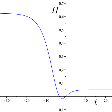
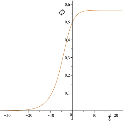
Figure 1: The functions $H(t)$, given by (18), and $\phi(t)=\phi_{+}(t)$ that correspond to a bounce solution. The values of parameter are $\xi=1$, $C_{2}=7/2$, $C_{1}=-3$, and $C_{0}=5/8$, and $t_{0}=2\ln(8/9)\simeq-0.235$.

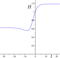
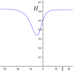
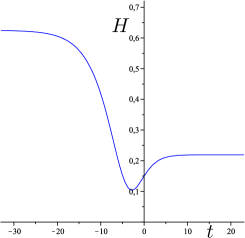
Figure 2: Non-monotonic functions $H(t)$, given by (18) that correspond to $\phi(t)$ plotted in Fig. 1. The values of parameter are $\xi=1$, $C_{2}=7/2$, and $C_{0}=5/8$, and $t_{0}=2\ln(8/9)$. The parameter $C_{1}=-1$ (left), $C_{1}=-2$ (middle), $C_{1}=-2.7$ (right).

The solution $\phi(t)$ in (20) is associated with different behaviors of the Hubble parameter. In Fig. 2, we plot a few non-monotonic $H(t)$ that corresponds to the same $\phi(t)$. We restrict ourselves to the case $C_{0}>0$ and $C_{2}>0$. One can see that the function $H(t)$ is not monotonic if and only if

$$\begin{split}-\frac{2\sqrt{(8\xi+1)C_{2}C_{0}}}{\sqrt{4\xi+1}}<C_{1}<0,&\quad\mbox{at}\ \phi(t)=\phi_{+}(t),\\ 0<C_{1}<\frac{2\sqrt{(8\xi+1)C_{2}C_{0}}}{\sqrt{4\xi+1}},&\quad\mbox{at}\ \phi(t)=\phi_{-}(t).\end{split}$$ (24)

In this case $\dot{H}=0$ at the point

$$t_{1}=t_{0}-\frac{4\xi+1}{4\xi C_{0}}\ln\left[\frac{\left(4(8\xi+1)C_{0}C_{2}-(4\xi+1)C_{1}^{2}\right)C_{2}}{(8\xi+1)C_{0}C_{1}^{2}}\right].$$ (25)

It is easy to see that the Hubble parameter (18) is invariant under transformation $C_{1}\rightarrow{}-C_{1}$ and $\phi(t)\rightarrow-\phi(t)$. By this reason $t_{1}$ is one and the same both for solutions tend to $\phi_{f_{+}}$, and for solutions tend to $\phi_{f_{-}}$.

Solutions described by (20) tend to a fixed point. Indeed, if $\omega>0$, then

$$\lim_{t\rightarrow\infty}\phi(t)=\phi_{f_{\pm}}\equiv\pm\frac{\sqrt{(8\xi+1)C_{0}}}{\sqrt{(4\xi+1)C_{2}}}\,.$$ (26)

In the case $\omega<0$, the function $\phi(t)$ tends to zero at late times. In the case $C_{0}=0$ the function $\phi(t)$ tends to zero as well. Therefore, the Hubble parameter tends to a constant value at late times for any case. So, the obtained solutions are asymptotically de Sitter ones. We choose $C_{0}>0$ and $\xi>0$, so $\omega>0$ as well. Thereby, to analyse stability of these solutions we should analyse the stability of de Sitter solutions with $\phi_{f\pm}$.

5 Stable solutions that tend to a fixed point

5.1 The Lyapunov stability

We consider the stability with respect to homogeneous isotropic perturbations. In other words, we consider system (16) and see stability with respect to the initial condition.

Let us remind few facts about stability [81, 82] of solutions for a general system of the first order autonomic equations

$$\dot{y}_{k}=F_{k}(y),\qquad k=1,2,\dots,N.$$ (27)

By definition a solution (a trajectory) $y_{0}(t)$ is attractive (stable) if

$$\|\tilde{y}(t)-y_{0}(t)\|\rightarrow 0\quad\mbox{at}\quad t\rightarrow\infty$$ (28)

for all solutions $\tilde{y}(t)$ that start close enough to $y_{0}(t)$.

We assume that $y(t)$ tends to a fixed point $y_{f}$. If all solutions of the dynamical system that start out near a fixed (equilibrium) point $y_{f}$,

$$F_{k}(y_{f})=0,\qquad k=1,2,\dots,N$$ (29)

stay near $y_{f}$ forever, then $y_{f}$ is a Lyapunov stable point. If all solutions that start out near the equilibrium point $y_{f}$ converge to $y_{f}$, then the fixed point $y_{f}$ is an asymptotically stable one. Asymptotic stability of fixed point means that solutions that start close enough to the equilibrium not only remain close enough but also eventually converge to the equilibrium.

The Lyapunov theorem [81, 82] states that to prove the stability of fixed point $y_{f}$ of nonlinear system (27) it is sufficient to prove the stability of this fixed point for the corresponding linearized system ($y$ is a column):

$$\dot{y}=Ay,\qquad A_{ik}=\frac{\partial F_{i}(y)}{\partial y_{k}}|_{y=y_{f}}.$$ (30)

The stability of the linear system means that real parts of all roots $\lambda_{k}$ of the characteristic equation

$$\det\left(A-\lambda I\right)|_{y=y_{f}}=0$$ (31)

are negative. Here $I$ is the identity matrix.

If at least one root of (31) is positive, then the fixed point is unstable. The case with pure imaginary eigenvalues of the Jacobian matrix of $F$ at the fixed point requires more specific treatment [83].

If a solution tends to a stable fixed point, then this solution is stable. Indeed, if a solution $y(t)$ tends to a fixed point $y_{f}$, then for any $\varepsilon>0$ there exist $t_{1}$ such that for all $t>t_{1}$ $|y(t)-y_{f}|<\varepsilon/2$. At the same time if functions $F_{k}$ are defined and continuous together with their partial derivatives, then solutions of system (27) continuously depend on the initial values [82]. It means that for any finite time $t_{1}$ and any $\varepsilon>0$ there exist such $\delta$ that $|y(t_{1})-\tilde{y}(t_{1})|<\varepsilon/2$ for all solutions $\tilde{y}(t)$ such that $|y(t_{0})-\tilde{y}(t_{0})|<\delta$. We denote the initial moment of time as $t_{0}$. It means that that for all solutions $\tilde{y}(t)$ we get $|\tilde{y}(t_{1})-y_{f}|<\varepsilon$, therefore, $|\tilde{y}(t)-y_{f}|<\varepsilon$ for all $t>t_{1}$ and $|y(t)-\tilde{y}(t)|<\varepsilon$ for all $t>t_{1}$, so $y(t)$ is a stable solution. Therefore, a solution $y_{0}(t)$ of (27), which tends to the fixed point $y_{f}$, is attractive if and only if the point $y_{f}$ is asymptotically stable.

The point $\phi=0$ is a singular point for system (16), so the above-mentioned arguments are not valid when one considers solutions that tend to this point. We restrict ourselves to consideration of solutions with $\omega>0$ and consider the Lyapunov stability of fixed points, corresponding to $\phi_{f\pm}$.

5.2 Stability conditions

To consider the stability of solutions of induced gravity models we denote $y(t)=(\phi(t),\psi(t),H(t))$. Let $y_{f}=(\phi_{f},\psi_{f},H_{f})$ is a fixed point. We get $\psi_{f}=0$. Also from Eqs. (13) and (15) we obtain:

$$V(\phi_{f})=3\xi\phi_{f}^{2}H_{f}^{2},\qquad V^{\prime}(\phi_{f})=12\xi\phi_{f}H_{f}^{2},$$ (32)

consequently,

$$V(\phi_{f})=\frac{1}{4}\phi_{f}V^{\prime}(\phi_{f}).$$ (33)

Let

$$\phi(t)=\phi_{f}+\varepsilon\phi_{1}(t),\qquad\psi(t)=\varepsilon\psi_{1}(t),\qquad H(t)=H_{f}+\varepsilon H_{1}(t).$$ (34)

To first order in $\varepsilon$ we obtain the following system of linear equations

$$\begin{split}\dot{\phi}_{1}&=\psi_{1},\\ \dot{\psi}_{1}&=\frac{1}{1+6\xi}\left[3\frac{V^{\prime}(\phi_{f})}{\phi_{f}}-V^{\prime\prime}(\phi_{f})\right]\phi_{1}-3H_{f}\psi_{1},\\ \dot{H}_{1}&=\frac{V^{\prime\prime}(\phi_{f})\phi_{f}-V^{\prime}(\phi_{f})}{(1+6\xi)\phi_{f}^{2}}\phi_{1}+\frac{4H_{f}}{(1+6\xi)\phi_{f}}\psi_{1}-\frac{24\xi H_{f}}{1+6\xi}H_{1}.\end{split}$$ (35)

With the result that we get the following matrix

$$A=\begin{array}[]{||c c c||}0&1&0\\[20.48596pt] \frac{36\xi H_{f}^{2}-V^{\prime\prime}(\phi_{f})}{1+6\xi}&-3H_{f}&0\\[20.48596pt] \frac{V^{\prime\prime}(\phi_{f})\phi_{f}-V^{\prime}(\phi_{f})}{(1+6\xi)\phi_{f}^{2}}&\quad\frac{4H_{f}}{(1+6\xi)\phi_{f}}&\quad{}-\frac{24\xi H_{f}}{1+6\xi}\\ \end{array}$$ (36)

and roots of Eq. (31) are as follows:

$$\begin{split}\lambda_{1}&={}-\frac{3}{2}H_{f}+\frac{\sqrt{9(22\xi+1)H_{f}^{2}-4V^{\prime\prime}(\phi_{f})}}{2\sqrt{1+6\xi}},\\ \lambda_{2}&={}-\frac{3}{2}H_{f}-\frac{\sqrt{9(22\xi+1)H_{f}^{2}-4V^{\prime\prime}(\phi_{f})}}{2\sqrt{1+6\xi}},\\ \lambda_{3}&={}-\frac{24\xi H_{f}}{1+6\xi}.\end{split}$$ (37)

So, we obtain the conditions on $H_{f}$ and $V^{\prime\prime}(\phi_{f})$ that are sufficient for the stability of de Sitter solutions in induced gravity models. If we assume $\xi>0$, then we get that a fixed point can be stable for $H_{f}>0$ only.

6 Stable solutions with a non-monotonic Hubble parameter

Let us consider the stability conditions for solutions, describing by formulae (18) and (20). Using (18), we get the following conditions on parameters of the potentials:

$$\lambda_{3}\quad\Leftrightarrow\quad H_{f}>0\quad\Leftrightarrow\quad\left\{\begin{array}[]{ll}C_{1}>-\frac{2(6\xi+1)\sqrt{C_{0}C_{2}}}{\sqrt{(4\xi+1)(8\xi+1)}},&\quad\mbox{for}\quad\phi_{f}=\phi_{f_{+}}\equiv\frac{\sqrt{(8\xi+1)C_{0}}}{\sqrt{(4\xi+1)C_{2}}},\\[20.48596pt] C_{1}<\frac{2(6\xi+1)\sqrt{C_{0}C_{2}}}{\sqrt{(4\xi+1)(8\xi+1)}},&\quad\mbox{for}\quad\phi_{f}=\phi_{f_{-}}\equiv{}-\frac{\sqrt{(8\xi+1)C_{0}}}{\sqrt{(4\xi+1)C_{2}}}.\end{array}\right.$$ (38)

If a solution tends to $\phi_{f_{+}}$, then

$$\begin{split}\lambda_{1+}&={}-\frac{3}{2}H_{f_{+}}+\frac{3\sqrt{C_{0}(8\xi+1)}}{2\sqrt{C_{2}(4\xi+1)}}\left(C_{1}+\frac{2(14\xi+3)\sqrt{C_{0}C_{2}}}{3\sqrt{(8\xi+1)(4\xi+1)}}\right),\\ \lambda_{2+}&={}-\frac{3}{2}H_{f_{+}}-\frac{3\sqrt{C_{0}(8\xi+1)}}{2\sqrt{C_{2}(4\xi+1)}}\left(C_{1}+\frac{2(14\xi+3)\sqrt{C_{0}C_{2}}}{3\sqrt{(8\xi+1)(4\xi+1)}}\right).\end{split}$$ (39)

Analogically, if a solution tends to $\phi_{f-}$, then

$$\begin{split}\lambda_{1-}&={}-\frac{3}{2}H_{f_{-}}+\frac{3\sqrt{C_{0}(8\xi+1)}}{2\sqrt{C_{2}(4\xi+1)}}\left(C_{1}-\frac{2(14\xi+3)\sqrt{C_{0}C_{2}}}{3\sqrt{(8\xi+1)(4\xi+1)}}\right),\\ \lambda_{2-}&={}-\frac{3}{2}H_{f_{-}}-\frac{3\sqrt{C_{0}(8\xi+1)}}{2\sqrt{C_{2}(4\xi+1)}}\left(C_{1}-\frac{2(14\xi+3)\sqrt{C_{0}C_{2}}}{3\sqrt{(8\xi+1)(4\xi+1)}}\right).\end{split}$$ (40)

We obtain that all $\lambda_{i}$ are real. Let us get conditions under that $\lambda_{i}$ are negative. The straightforward calculations show that

$$\lambda_{1+}={}-\frac{4\xi}{4\xi+1}C_{0}\,.$$ (41)

We consider the case $C_{0}>0$ and $\xi>0$, hence, $\lambda_{1+}<0$. So, the stability of the fixed point $\phi_{f_{+}}$ depends on sign of

$$\lambda_{2+}={}-3\frac{\sqrt{(8\xi+1)C_{0}}}{\sqrt{(4\xi+1)C_{2}}}C_{1}-\frac{32\xi+6}{4\xi+1}C_{0}\,.$$ (42)

We see that

$$\lambda_{2_{+}}<0\qquad\Leftrightarrow\qquad C_{1}>{}-\frac{2(16\xi+3)\sqrt{C_{0}C_{2}}}{3\sqrt{(8\xi+1)(4\xi+1)}}.$$ (43)

To explore the stability of the stable point $\phi_{f_{-}}$, we consider $\lambda_{i_{\pm}}$ as functions of the parameter $C_{1}$ and take notice that $\lambda_{1_{-}}(C_{1})=\lambda_{2_{+}}(-C_{1})$ and $\lambda_{2_{-}}(C_{1})=\lambda_{1_{+}}(-C_{1})$. Consequently, we get

$$\lambda_{1-}=3\frac{\sqrt{(8\xi+1)C_{0}}}{\sqrt{(4\xi+1)C_{2}}}C_{1}-\frac{32\xi+6}{4\xi+1}C_{0}\,,\qquad\lambda_{2-}={}-\frac{4\xi}{4\xi+1}C_{0}\,.$$ (44)

$$\lambda_{1_{-}}<0\qquad\Leftrightarrow\qquad C_{1}<\frac{2(16\xi+3)\sqrt{C_{0}C_{2}}}{3\sqrt{(8\xi+1)(4\xi+1)}}.$$ (45)

Now we are ready to analyse the stability of the fixed points. Let us start with $\phi_{f_{+}}$. We consider only the case $C_{0}>0$, $C_{2}>0$ and $\xi>0$. We see that $\lambda_{1_{+}}<0$ and $\lambda_{3_{+}}<0$ is a more strong restriction on $C_{1}$ than $\lambda_{2_{+}}<0$. Therefore, the fixed point $\phi_{f_{+}}$ is stable at $\lambda_{2_{+}}<0$. The analogous reasoning gives that $\phi_{f_{-}}$ is stable at $\lambda_{1_{-}}<0$.

Now let us analyse the stability of solutions with nonmonotonic Hubble parameter. For such a solution that tends to a stable point $\phi_{f_{+}}$ condition (43) should be satisfied. So, we get a such stable solution at

$$\begin{split}{}-\frac{2(16\xi+3)\sqrt{C_{0}C_{2}}}{3\sqrt{(8\xi+1)(4\xi+1)}}<C_{1}<0,&\quad\phi(t)=\phi_{+}(t),\\ 0<C_{1}<\frac{2(16\xi+3)\sqrt{C_{0}C_{2}}}{3\sqrt{(8\xi+1)(4\xi+1)}},&\quad\phi(t)=\phi_{-}(t).\end{split}$$ (46)

For example, we get that at $\xi=1$, $C_{2}=7/2$ and $C_{0}=5/8$, solutions are stable if $C_{1}>-19\sqrt{7}/18\approx-2.7927$. Therefore, solutions, presented in Fig. 2, are stable, whereas the bounce solution that we plot in Fig. 1 is unstable.

7 Conclusion

We have analysed the stability of kink-type solutions for the induced gravity models in the FLRW metric. Using the Lyapunov theorem we have found sufficient conditions of stability. The obtained results allow us to prove that the exact solutions, with non-monotonic behaviors of the Hubble parameter, found in [69], are stable if condition (46) is satisfied.

Our study of the stability of isotropic solutions with nonmonotonic behaviors of the Hubble parameter shows that it is possible to obtain stable solutions with increasing Hubble parameter, in particular, the bounce solutions.

We have analysed the stability of solutions, specifying a form of fluctuations. It is interesting to know whether these solutions are stable under the deformation of the FLRW metric to an anisotropic one, for example, to the Bianchi I metric. Also, it is interesting to check the possibility to get a stable bounce solution in the induced gravity model. This will be a subject of our future investigations.

Acknowledgements.

The authors are grateful to the organizers of the Second Russian-Spanish Congress ”Particle and Nuclear Physics at all scales, Astroparticle Physics and Cosmology” for the hospitality and the financial support. This work is supported in part by the Russian Ministry of Education and Science under grant NSh-3042.2014.2 and by the RFBR grant 14-01-00707.

References

- [1] S. Perlmutter et al. [SNCP Collaboration], Measurements of Omega and Lambda from 42 High-Redshift Supernovae, Astrophys. J. 517 (1999) 565–586 (arXiv:astro-ph/9812133)
-
[2]
A.G. Riess et al. [Supernova Search Team Collaboration],
Observational Evidence from Supernovae for an Accelerating Universe and a Cosmological Constant,
Astron. J. 116 (1998) 1009–1038 (arXiv:astro-ph/9805201);
A.G. Riess et al. [Supernova Search Team Collaboration], Type Ia supernova discoveries at from the Hubble Space Telescope: Evidence for past deceleration and constraints on dark energy evolution, Astrophys. J. 607 (2004) 665–687 (arXiv:astro-ph/0402512);
P. Astier et al., The Supernova Legacy Survey: Measurement of , and from the First Year Data Set, Astron. Astrophys. 447 (2006) 31–48 (arXiv:astro-ph/0510447) -
[3]
D.N. Spergel et al. [WMAP Collaboration],
First Year Wilkinson Microwave Anisotropy Probe (WMAP) Observations:
Determination of Cosmological Parameters,
Astrophys. J. Suppl. 148 (2003) 175–194
(arXiv:astro-ph/0302209);
D.N. Spergel et al. [WMAP Collaboration], Wilkinson Microwave Anisotropy Probe (WMAP) three year results: Implications for cosmology, Astrophys. J. Suppl. 170 (2007) 377 (arXiv:astro-ph/0603449);
E. Komatsu et al. [WMAP Collaboration], Five-Year Wilkinson Microwave Anisotropy Probe (WMAP) Observations:Cosmological Interpretation, Astrophys. J. Suppl. 180 (2009) 330–376 (arXiv:0803.0547);
E. Komatsu et al. [WMAP Collaboration], Seven-Year Wilkinson Microwave Anisotropy Probe (WMAP) Observations: Cosmological Interpretation, Astrophys. J. Suppl. 192 (2011) 18 (arXiv:1001.4538) -
[4]
M. Tegmark et al. [SDSS Collaboration],
Cosmological parameters from SDSS and WMAP,
Phys. Rev. D 69 (2004) 103501
(arXiv:astro-ph/0310723);
M. Tegmark et al. [SDSS collaboration], The 3D power spectrum of galaxies from the SDS, Astroph. J. 606 (2004) 702–740 (arXiv:astro-ph/0310725);
U. Seljak et al. [SDSS Collaboration], Cosmological parameter analysis including SDSS Ly-alpha forest and galaxy bias: Constraints on the primordial spectrum of fluctuations, neutrino mass, and dark energy, Phys. Rev. D 71 (2005) 103515 (arXiv:astro-ph/0407372);
D.J. Eisenstein et al. [SDSS Collaboration], Detection of the Baryon Acoustic Peak in the Large-Scale Correlation Function of SDSS Luminous Red Galaxies, Astrophys. J. 633 (2005) 560–574 (arXiv:astro-ph/0501171) - [5] W.M. Wood-Vasey et al. [ESSENCE Collaboration], Observational Constraints on the Nature of the Dark Energy: First Cosmological Results from the ESSENCE Supernova Survey, Astrophys. J. 666 (2007) 694–715 (arXiv:astro-ph/0701041)
- [6] B. Jain and A. Taylor, Cross-correlation Tomography: Measuring Dark Energy Evolution with Weak Lensing, Phys. Rev. Lett. 91 (2003) 141302 (arXiv:astro-ph/0306046)
- [7] A. Bernui, B. Mota, M.J. Reboucas, and R. Tavakol, Mapping large-scale anisotropy in the WMAP data, Astron. Astrophys. 464 (2007) 479–485 (arXiv:astro-ph/0511666)
-
[8]
P.A.R. Ade, et. al. [Planck Collaboration], Planck 2013 results. XVI. Cosmological parameters, arXiv:1303.5076;
P.A.R. Ade, et. al. [Planck Collaboration], Planck 2013 results. XXII. Constraints on inflation, arXiv:1303.5082;
P.A.R. Ade, et. al. [Planck Collaboration], Planck 2013 Results. XXIV. Constraints on primordial non-Gaussianity, arXiv:1303.5084 -
[9]
T. Padmanabhan,
Cosmological constant — the weight of the vacuum,
Phys. Rept. 380 (2003) 235–320
(arXiv:hep-th/0212290);
P. Frampton, Dark Energy — a Pedagogic Review, arXiv:astro-ph/0409166;
A.D. Dolgov, Cosmology and Elementary Particles, or Celestial Mysteries, Phys. Part. Nucl. 43 (2012) 273–293;
K. Bamba, S. Capozziello, S. Nojiri, and S.D. Odintsov, Dark energy cosmology: the equivalent description via different theoretical models and cosmography tests, Astrophys. Space Science 342 (2012) 155–228 (arXiv:1205.3421) - [10] E.J. Copeland, M. Sami, and Sh. Tsujikawa, Dynamics of dark energy, Int. J. Mod. Phys. D 15 (2006) 1753–1936 (arXiv:hep-th/0603057)
- [11] C. Wetterich, Modified gravity and coupled quintessence, arXiv:1402.5031
- [12] Sh. Tsujikawa, Quintessence: A Review, Class. Quant. Grav. 30 (2013) 214003 (arXiv:1304.1961)
-
[13]
A.A. Starobinsky,
Relict Gravitation Radiation Spectrum and Initial State of the Universe (In Russian),
JETP Lett. 30 (1979) 682 [Pisma Zh. Eksp. Teor. Fiz. 30 (1979) 719–723];
A.A. Starobinsky, A New Type of Isotropic Cosmological Models Without Singularity, Phys. Lett. B 91 (1980) 99–102;
A.A. Starobinsky, Lect. Notes in Phys. 246 (1986) 107 - [14] V.F. Mukhanov and G.V. Chibisov, Quantum Fluctuation and Nonsingular Universe (In Russian), JETP Lett. 33 (1981) 532–535, [Pisma Zh. Eksp. Teor. Fiz. 33 (1981) 549–553].
- [15] A.H. Guth, The Inflationary Universe: A Possible Solution to the Horizon and Flatness Problems, Phys. Rev. D 23 (1981) 347
-
[16]
A.D. Linde,
A New Inflationary Universe Scenario: A Possible Solution of the Horizon, Flatness, Homogeneity, Isotropy and Primordial Monopole Problems, Phys. Lett. B 108 (1982) 389;
A.D. Linde, Chaotic Inflation, Phys. Lett. B 129 (1983) 177;
A.D. Linde, Particle Physics and Inflationary Cosmology, Chur, Switzerland: Harwood, 1990 - [17] A. Albrecht and P.J. Steinhardt, Cosmology for Grand Unified Theories with Radiatively Induced Symmetry Breaking, Phys. Rev. Lett. 48 (1982) 1220
-
[18]
J.E. Lidsey, A.R. Liddle, E.W. Kolb, E.J. Copeland, T. Barreiro, and M. Abney,
Reconstructing the inflaton potentialan overview,
Rev. Mod. Phys. 69 (1997) 373–410 (arXiv:astro-ph/9508078);
M.V. Libanov, V.A. Rubakov and P.G. Tinyakov, Cosmology with nonminimal scalar field: Graceful entrance into inflation, Phys. Lett. B 442 (1998) 63 (arXiv:hep-ph/9807553);
C.M. Peterson, M. Tegmark, Testing Two-Field Inflation, Phys. Rev. D 83 (2011) 023522 (arXiv:1005.4056);
Shi Pi, M. Sasaki, Curvature perturbation spectrum in two-field inflation with a turning trajectory, J. Cosmol. Astropart. Phys. 1210 (2012) 051 (arXiv:1205.0161) - [19] U. Alam, V. Sahni, T.D. Saina, and A.A. Starobinsky, Is there Supernova Evidence for Dark Energy Metamorphosis?, Mon. Not. R. Astron. Soc. 354 (2004) 275–291 (arXiv:astro-ph/0311364)
- [20] Zong-Kuan Guo, Yun-Song Piao, Xinmin Zhang, Yuan-Zhong Zhang, Cosmological Evolution of a Quintom Model of Dark Energy, Phys. Lett. B 608 (2005) 177–182 (arXiv:astro-ph/0410654)
-
[21]
I.Ya. Aref’eva, A.S. Koshelev, and S.Yu. Vernov,
Crossing the barrier in the D3-brane dark energy model,
Phys. Rev. D 72 (2005) 064017 (arXiv:astro-ph/0507067);
S.Yu. Vernov, Construction of exact solutions in two-field cosmological models, Theor. Math. Phys. 155 (2008) 544–556 [Teor. Mat. Fiz. 155 (2008) 47–61] (arXiv:astro-ph/0612487) -
[22]
R. Lazkoz, G. León, and I. Quiros,
Quintom cosmologies with arbitrary potentials,
Phys. Lett. B 649 (2007)
103–110 (arXiv:astro-ph/0701353);
R. Lazkoz and G. León, Quintom cosmologies admitting either tracking or phantom attractors, Phys. Lett. B 638 (2006) 303–309 (arXiv:astro-ph/0602590) - [23] Yi-Fu Cai, E.N. Saridakis, M.R. Setare, and Jun-Qing Xia, Quintom Cosmology: theoretical implications and observations, Phys. Rep. 493 (2010) 1–60 (arXiv:0909.2776)
- [24] Hongsheng Zhang, Crossing the phantom divide, arXiv:0909.3013
- [25] V.A. Rubakov, The Null Energy Condition and its violation, arXiv:1401.4024
- [26] S. Nesseris, L. Perivolaropoulos, Crossing the Phantom Divide: Theoretical Implications and Observational Status, J. Cosmol. Astropart. Phys. 0701 (2007) 018 (arXiv:astro-ph/0610092)
- [27] I.Ya. Aref’eva, Nonlocal String Tachyon as a Model for Cosmological Dark Energy, AIP Conf. Proc. 826 (2006) 301–311, arXiv:astro-ph/0410443
- [28] I.Ya. Aref’eva, A.S. Koshelev, and S.Yu. Vernov, Exactly Solvable SFT Inspired Phantom Model, Theor. Math. Phys. 148 (2006) 895–909 [Teor. Mat. Fiz. 148 (2006) 23–41] (arXiv:astro-ph/0412619)
- [29] B. McInnes, The Phantom divide in string gas cosmology, Nucl.Phys. B 718 (2005) 55–82 (arXiv:hep-th/0502209)
- [30] Z.-K. Guo, Y.-S. Piao, and Y.-Zh. Zhang, Attractor Behavior of Phantom Cosmology, Phys. Lett. B 594 (2004) 247–251 (arXiv:astro-ph/0404225)
- [31] I.Ya. Aref’eva, A.S. Koshelev, and S.Yu. Vernov, Stringy Dark Energy Model with Cold Dark Matter, Phys. Lett. B 628 (2005) 1–10 (arXiv:astro-ph/0505605)
- [32] I.Ya. Aref’eva, N.V. Bulatov, L.V. Joukovskaya, and S.Yu. Vernov, The NEC Violation and Classical Stability in the Bianchi I Metric, Phys. Rev. D 80 (2009) 083532 (arXiv:0903.5264)
- [33] Y. Fujii and K. Maeda, The Scalar–Tensor Theory of Gravitation, Cambridge University Press, Cambridge, 2004
-
[34]
S. Nojiri and S.D. Odintsov,
Modified gravity and its reconstruction from the universe expansion history,
J. Phys. Conf. Ser. 66 (2007) 012005 (arXiv:hep-th/0611071);
S. Nojiri and S.D. Odintsov, Introduction to modified gravity and gravitational alternative for dark energy, Int. J. Geom. Meth. Mod. Phys. 4 (2007) 115–146 (arXiv:hep-th/0601213);
S. Nojiri and S.D. Odintsov, Unified cosmic history in modified gravity: from theory to Lorentz non-invariant models, Phys. Rept. 505 (2011) 59–144 (arXiv:1011.0544) - [35] S. Capozziello and V. Faraoni, Beyond Einstein Gravity: A Survey of Gravitational Theories for Cosmology and Astrophysics, Fund. Theor. Phys. 170, Springer, New York, 2011
- [36] S. Capozziello and M. De Laurentis, Extended Theories of Gravity, Phys. Rep. 509 (2011) 167–321 (arXiv:1108.6266)
- [37] A. de Felice and Sh. Tsujikawa, Theories, Living Rev. Rel. 13 (2010) 3 (arXiv:1002.4928)
- [38] S. Deser and R.P. Woodard, Nonlocal Cosmology, Phys. Rev. Lett. 99 (2007) 111301 (arXiv:0706.2151)
- [39] C. Deffayet and R.P. Woodard, Reconstructing the Distortion Function for Nonlocal Cosmology, J. Cosmol. Astropart. Phys. 0908 (2009) 023 (arXiv:0904.0961)
-
[40]
S. Park and S. Dodelson,
Structure formation in a nonlocally modified gravity model,
Phys. Rev. D 87 (2013) 024003 (arXiv:1209.0836);
S. Dodelson and S. Park, Nonlocal Gravity and Structure in the Universe, arXiv:1310.4329 - [41] S. Deser and R.P. Woodard, Observational Viability and Stability of Nonlocal Cosmology, J. Cosmol. Astropart. Phys. 1311 (2013) 036 (arXiv:1307.6639)
-
[42]
S. Foffa, M. Maggiore and E. Mitsou,
Apparent ghosts and spurious degrees of freedom in non-local theories,
arXiv:1311.3421;
S. Foffa, M. Maggiore and E. Mitsou, Cosmological dynamics and dark energy from non-local infrared modifications of gravity, arXiv:1311.3435 - [43] R.P. Woodard, Nonlocal Models of Cosmic Acceleration, Found. Phys. 44 (2014) 213–233 (arXiv:1401.0254)
- [44] S. Nojiri and S.D. Odintsov, Modified non-local-F(R) gravity as the key for the inflation and dark energy, Phys. Lett. B 659 (2008) 821–826 (arXiv:0708.0924)
- [45] S. Jhingan, S. Nojiri, S.D. Odintsov, M. Sami, I. Thongkool, and S. Zerbini, Phantom and non-phantom dark energy: The cosmological relevance of non-locally corrected gravity, Phys. Lett. B 663 (2008) 424–428 (arXiv:0803.2613)
- [46] T.S. Koivisto, Dynamics of Nonlocal Cosmology, Phys. Rev. D 77 (2008) 123513 (arXiv:0803.3399) T.S. Koivisto, Newtonian limit of nonlocal cosmology, Phys. Rev. D 78 (2008) 123505 (arXiv:0807.3778)
-
[47]
N.A. Koshelev,
Comments on scalar-tensor representation of nonlocally corrected gravity,
Grav. Cosmol. 15 (2009) 220–223 (arXiv:0809.4927);
K.A. Bronnikov and E. Elizalde, Spherical systems in models of nonlocally corrected gravity, Phys. Rev. D 81 (2010) 044032 (arXiv:0910.3929);
A.J. López-Revelles and E. Elizalde, Universal procedure to cure future singularities of dark energy models, Gen. Rel. Grav. 44 (2012) 751–770 (arXiv:1104.1123);
J. Kluson, Non-Local Gravity from Hamiltonian Point of View, J. High Energy Phys. 1109 (2011) 001 (arXiv:1105.6056) -
[48]
S. Nojiri, S.D. Odintsov, M. Sasaki and Y.l. Zhang,
Screening of cosmological constant in non-local gravity,
Phys. Lett. B 696 (2011) 278–282
(arXiv:1010.5375);
K. Bamba, S. Nojiri, S.D. Odintsov, and M. Sasaki, Screening of cosmological constant for De Sitter Universe in non-local gravity, phantom-divide crossing and finite-time future singularities, Gen. Rel. Grav. 44 (2012) 1321–1356 (arXiv:1104.2692);
Y.l. Zhang and M. Sasaki, Screening of cosmological constant in non-local cosmology, Int. J. Mod. Phys. D 21 (2012) 1250006 (arXiv:1108.2112) -
[49]
E. Elizalde, E.O. Pozdeeva, and S.Yu. Vernov,
De Sitter universe in nonlocal gravity,
Phys. Rev. D 85 (2012) 044002 (arXiv:1110.5806);
E. Elizalde, E.O. Pozdeeva, and S.Yu. Vernov, Stability of de Sitter Solutions in Non-local Cosmological Models, Proceedings of Science, PoS(QFTHEP2011)038, 2012 (arXiv:1202.0178);
S.Yu. Vernov, Nonlocal Gravitational Models and Exact Solutions, Phys. Part. Nucl. 43 (2012) 694–696 (arXiv:1202.1172);
E. Elizalde, E.O. Pozdeeva, and S.Yu. Vernov, Reconstruction Procedure in Nonlocal Models, Class. Quantum Grav. 30 (2013) 035002 (arXiv:1209.5957);
E. Elizalde, E.O. Pozdeeva, S.Yu. Vernov, and Y-l. Zhang, Cosmological Solutions of a Nonlocal Model with a Perfect Fluid, J. Cosmol. Astropart. Phys. 1307 (2013) 034 (arXiv:1302.4330) - [50] F. Bezrukov, D. Gorbunov, Light inflaton after LHC8 and WMAP9 results, J. High Energy Phys. 1307 (2013) 140 (arXiv:1303.4395)
- [51] R. Kallosh, A. Linde, Superconformal generalization of the chaotic inflation model , J. Cosmol. Astropart. Phys. 1306 (2013) 027 (arXiv:1306.3211)
- [52] F.L. Bezrukov and M. Shaposhnikov, The Standard Model Higgs boson as the inflaton, Phys. Lett. B 659 (2008) 703 (arXiv:0710.3755)
-
[53]
F. Bezrukov, D. Gorbunov and M. Shaposhnikov,
On initial conditions for the Hot Big Bang,
J. Cosmol. Astropart. Phys. 0906 (2009) 029 (arXiv:0812.3622);
F.L. Bezrukov and D.S. Gorbunov, Distinguishing between -inflation and Higgs-inflation, Phys. Lett. B 713 (2012) 365 (arXiv:1111.4397) -
[54]
A.O. Barvinsky, A.Y. Kamenshchik, and A.A. Starobinsky,
Inflation scenario via the Standard Model Higgs boson and LHC
J. Cosmol. Astropart. Phys. 0811 (2008) 021 [arXiv:0809.2104];
A.O. Barvinsky, A.Y. Kamenshchik, C. Kiefer, A.A. Starobinsky, and C.F. Steinwachs, Asymptotic freedom in inflationary cosmology with a non-minimally coupled Higgs field, J. Cosmol. Astropart. Phys. 0912 (2009) 003 (arXiv:0904.1698);
A.O. Barvinsky, A.Y. Kamenshchik, C. Kiefer, A.A. Starobinsky, and C.F. Steinwachs, Higgs boson, renormalization group, and cosmology, Eur. Phys. J. C 72 (2012) 2219 (arXiv:0910.1041) -
[55]
J. Garcia-Bellido, D.G. Figueroa, and J. Rubio,
Preheating in the Standard Model with the Higgs-Inflaton coupled to gravity,
Phys. Rev. D 79 (2009) 063531 (arXiv:0812.4624);
R.N. Lerner and J. McDonald, Higgs Inflation and Naturalness, J. Cosmol. Astropart. Phys. 1004 (2010) 015 (arXiv:0912.5463) - [56] A.O. Barvinsky, A.Y. Kamenshchik, C. Kiefer, and C.F. Steinwachs, The Higgs field as an inflaton Tunneling cosmological state revisited: Origin of inflation with a non-minimally coupled Standard Model Higgs inflaton, Phys. Rev. D 81 (2010) 043530 (arXiv:0911.1408)
- [57] F. Bezrukov, The Higgs field as an inflaton, Class. Quantum Grav. 30 (2013) 214001 (arXiv:1307.0708)
- [58] F. Cooper and G. Venturi, Cosmology and broken scale invariance, Phys. Rev. D 24 (1981) 3338
-
[59]
D.I. Kaiser,
Induced-gravity Inflation and the Density Perturbation Spectrum,
Phys. Lett. B 340 (1994) 23–28 (arXiv:astro-ph/9405029);
D.I. Kaiser, Primordial spectral indices from generalized Einstein theories, Phys. Rev. D 52 (1995) 4295 (arXiv:astro-ph/9408044) - [60] A.Yu. Kamenshchik, I.M. Khalatnikov, A.V. Toporensky, Complex inflaton field in quantum cosmology, Int. J. Mod. Phys. D 6 (1997) 649–672 (arXiv:gr-qc/9801039)
-
[61]
E. Elizalde, Sh. Nojiri, and S.D. Odintsov,
Late-time cosmology in (phantom) scalar-tensor theory: dark energy and the cosmic speed-up,
Phys. Rev. D 70 (2004) 043539 (arXiv:hep-th/0405034);
E. Elizalde, Sh. Nojiri, S.D. Odintsov, D. Saez-Gomez and V. Faraoni, Reconstructing the universe history, from inflation to acceleration, with phantom and canonical scalar fields, Phys. Rev. D 77 (2008) 106005 (arXiv:0803.1311);
D. Saez-Gomez, Scalar-tensor theory with Lagrange multipliers: a way of understanding the cosmological constant problem, and future singularities, Phys. Rev. D 85 (2012) 023009 (arXiv:1110.6033) -
[62]
A. Cerioni, F. Finelli, A. Tronconi and G. Venturi,
Inflation and Reheating in Induced Gravity,
Phys. Lett. B 681 (2009) 383–386 (arXiv:0906.1902);
A. Cerioni, F. Finelli, A. Tronconi and G. Venturi, Inflation and Reheating in Spontaneously Generated Gravity, Phys. Rev. D 81 (2010) 123505 (arXiv:1005.0935);
A. Tronconi and G. Venturi, Quantum Back-Reaction in Scale Invariant Induced Gravity Inflation, Phys. Rev. D 84 (2011) 063517 (arXiv:1011.39580) -
[63]
M. Szydlowski and O. Hrycyna,
Scalar field cosmology in the energy phase-space – unified description of dynamics,
J. Cosmol. Astropart. Phys. 0901 (2009) 039 (arXiv:0811.1493);
O. Hrycyna and M. Szydlowski, Dynamical complexity of the Brans-Dicke cosmology, J. Cosmol. Astropart. Phys. 1312 (2013) 016 (arXiv:1310.1961);
M. Szydlowski, O. Hrycyna and A. Stachowski, Scalar field cosmology - geometry of dynamics, Int. J. Geom. Meth. Mod. Phys. 11 (2014) 1460012 (arXiv:1308.4069) - [64] A.Y. Kamenshchik, A. Tronconi and G. Venturi, Dynamical Dark Energy and Spontaneously Generated Gravity, Phys. Lett. B 713 (2012) 358 (arXiv:1204.2625)
-
[65]
J.L. Cervantes-Cota, R. de Putter, and E.V. Linder,
Induced Gravity and the Attractor Dynamics of Dark Energy/Dark Matter,
J. Cosmol. Astropart. Phys. 1012 (2010) 019 (arXiv:1010.2237);
J.L. Cervantes-Cota and H. Dehnen, Induced gravity inflation in the SU(5) GUT, Phys. Rev. D 51 (1995) 395 (arXiv:astro-ph/9412032);
J.L. Cervantes-Cota and H. Dehnen, Induced gravity inflation in the standard model of particle physics, Nucl. Phys. B 442 (1995) 391 (arXiv:astro-ph/9505069) - [66] A.Yu. Kamenshchik, A. Tronconi, and G. Venturi, Reconstruction of scalar potentials in induced gravity and cosmology, Phys. Lett. B 702 (2011) 191–196 (arXiv:1104.2125)
- [67] M. Sami, M. Shahalam, M. Skugoreva, and A. Toporensky, Cosmological dynamics of non-minimally coupled scalar field system and its late time cosmic relevance, Phys. Rev. D 86 (2012) 103532 (arXiv:1207.6691)
- [68] I.Ya. Aref’eva, N.V. Bulatov, R.V. Gorbachev, S.Yu. Vernov, Non-minimally Coupled Cosmological Models with the Higgs-like Potentials and Negative Cosmological Constant, Class. Quant. Grav. 31 (2014) 065007 (arXiv:1206.2801)
- [69] A.Yu. Kamenshchik, A. Tronconi, G. Venturi, and S.Yu. Vernov, Reconstruction of Scalar Potentials in Modified Gravity Models, Phys. Rev. D 87 (2013) 063503 (arXiv:1211.6272)
- [70] A.Yu. Kamenshchik, E.O. Pozdeeva, A. Tronconi, G. Venturi and S.Yu. Vernov, Integrable cosmological models with non-minimally coupled scalar fields, Class. Quant. Grav. 31 (2014) to be published, arXiv:1312.3540
-
[71]
A.G. Muslimov,
On the Scalar Field Dynamics in a Spatially Flat Friedman Universe,
Class. Quant. Grav. 7 (1990) 231–237,
D.S. Salopek and J.R. Bond, Nonlinear evolution of long-wavelength metric fluctuations in inflationary models, Phys. Rev. D 42 (1990) 3936–3962,
V.M. Zhuravlev, S.V. Chervon and V.K. Shchigolev, New classes of exact solutions in inflationary cosmology, J. Exp. Theor. Phys. 87 (1998) 223;
P.K. Townsend, Hamilton-Jacobi Mechanics from Pseudo-Supersymmetry, Class. Quant. Grav. 25 (2008) 045017 (arXiv:0710.5178);
A.V. Yurov, V.A. Yurov, S.V. Chervon, and M. Sami, Total energy potential as a superpotential in integrable cosmological models, Theor. Math. Phys. 166 (2011) 259–269;
A.Yu. Kamenshchik and S. Manti, Scalar field potentials for closed and open cosmological models, Gen. Rel. Grav. 44 (2012) 2205–2214 (arXiv:1111.5183);
H.-Ch. Kim, Exact solutions in Einstein cosmology with a scalar field, Mod. Phys. Lett. A 28 (2013) 1350089 (arXiv:1211.0604) -
[72]
D. Bazeia, C.B. Gomes, L. Losano, R. Menezes,
First-order formalism and dark energy,
Phys. Lett. B 633 (2006)
415–419 (arXiv:astro-ph/0512197);
D. Bazeia, L. Losano, R. Rosenfeld, First-order formalism for dust, Eur. Phys. J. C 55 (2008) 113–117 (arXiv:astro-ph/0611770) -
[73]
A.A. Andrianov, F. Cannata, A.Yu. Kamenshchik, and D. Regoli,
Reconstruction of scalar potentials in two-field cosmological models,
J. Cosmol. Astropart. Phys. 0802 (2008) 015 (arXiv:0711.4300);
M.R. Setare, J. Sadeghi, First-order formalism for the quintom model of dark energy, Int. J. Theor. Phys. 47 (2008) 3219–3225 (arXiv:0805.1117) - [74] I.Ya. Aref’eva, N.V. Bulatov, and S.Yu. Vernov, Stable exact solutions in cosmological models with two scalar fields, Theor. Math. Phys. 163 (2010) 788–803 (arXiv:0911.5105)
- [75] V.K. Shchigolev and M.P. Rotova, Cosmological model of interacting tachyon field, Mod. Phys. Lett. A 27 (2012) 1250086 (arXiv:1203.5030)
- [76] T. Harko, F.S.N. Lobo, and M.K. Mak, Arbitrary scalar field and quintessence cosmological models, Eur. Phys. J. C 74 2784 (arXiv:1310.7167)
-
[77]
A. Brandhuber and K. Sfetsos,
Nonstandard compactifications with mass gaps and Newton’s law,
J. High Energy Phys. 9910 (1999) 013 (arXiv:hep-th/9908116);
O. DeWolfe, D.Z. Freedman, S.S. Gubser, A. Karch, Modeling the fifth dimension with scalars and gravity, Phys. Rev. D 62 (2000) 046008 (arXiv:hep-th/9909134) - [78] A.S. Mikhailov, Yu.S. Mikhailov, M.N. Smolyakov, I.P. Volobuev, Constructing stabilized brane world models in five-dimensional Brans-Dicke theory, Class. Quantum Grav. 24 (2007) 231–242 (arXiv:hep-th/0602143) M.N. Smolyakov and I.P. Volobuev, Single-brane world with stabilized extra dimension, Int. J. Mod. Phys. A 23 (2008) 761 (arXiv:0705.4495)
- [79] U. Gursoy, E. Kiritsis, L. Mazzanti and F. Nitti, Holography and Thermodynamics of 5D Dilaton-gravity, J. High Energy Phys. 0905 (2009) 033 (arXiv:0812.0792)
- [80] I.Ya. Aref’eva, E.O. Pozdeeva and T.O. Pozdeeva, Holographic estimation of multiplicity and membranes collision in modified spaces , arXiv:1401.1180.
- [81] A.M. Lyapunov, Stability of motion, Academic Press, New-York and London, 1966 (in English); A.M. Lyapunov, General problem of stability of motion, GITTL, Moscow–Leningrad, 1950 (in Russian)
- [82] L.S. Pontryagin, Ordinary Differential Equations, Adiwes International Series in Mathematics. Addison-Wesley Publ. Comp., London–Paris, 1962 (in English), ”Nauka”, Moscow, 1982 (in Russian)
- [83] B.I. Arnold and Yu.S. Ilyashenko, Ordinary Differential equations, Itogi Nauki, vol. 1, 1985