Exactly solvable models of nuclei

“If politics is the art of the possible, research is surely the art of the soluble [1]”

1 Introduction

The atomic nucleus is a many-body system predominantly governed by a complex and effective in-medium nuclear interaction and as such exhibits a rich spectrum of properties. These range from independent nucleon motion in nuclei near closed shells, to correlated two-nucleon pair formation as well as collective effects characterized by vibrations and rotations resulting from the cooperative motion of many nucleons.

The present-day theoretical description of the observed variety of nuclear excited states has two possible microscopic approaches as its starting point. Self-consistent mean-field methods start from a given nucleon–nucleon effective force or energy functional to construct the average nuclear field; this leads to a description of collective modes starting from the correlations between all neutrons and protons constituting a given nucleus [2]. The spherical nuclear shell model, on the other hand, includes all possible interactions between neutrons and protons outside a certain closed-shell configuration [3]. Both approaches make use of numerical algorithms and are therefore computer intensive.

In this paper a review is given of a class of sub-models of both approaches, characterized by the fact that they can be solved exactly, highlighting in the process a number of generic results related to both the nature of pair-correlated systems as well as collective modes of motion in the atomic nucleus. Exactly solvable models necessarily are of a schematic character, valid for specific nuclei only. But they can be used as a reference or ‘bench mark’ in the study of data over large regions of the nuclear chart (series of isotopes or isotones) with more realistic models using numerical approaches. The emphasis here is on the exactly solvable models themselves rather than on the comparison with data. The latter aspect of exactly solvable models is treated in several of the books mentioned at the end of this review (e.g., references [115, 116, 117, 118]).

2 An algebraic formulation of the quantal $n$-body problem

Symmetry techniques and algebraic methods are not confined to certain models in nuclear physics but can be applied generally to find particular solutions of the quantal $n$-body problem. How that comes about is explained in this section.

To describe the stationary properties of an $n$-body system in non-relativistic quantum mechanics, one needs to solve the time-independent Schrödinger equation which reads

$$\hat{H}\Psi(\xi_{1},\dots,\xi_{n})=E\Psi(\xi_{1},\dots,\xi_{n}),$$ (1)

where $\hat{H}$ is the many-body hamiltonian

$$\hat{H}=\sum_{k=1}^{n}\left(\frac{\hat{p}_{k}^{2}}{2m_{k}}+\hat{V}_{1}(\xi_{k})\right)+\sum_{k<l}\hat{V}_{2}(\xi_{k},\xi_{l})+\sum_{k<l<m}\hat{V}_{3}(\xi_{k},\xi_{l},\xi_{m})+\cdots,$$ (2)

with $m_{k}$ the mass and $\hat{p}_{k}^{2}/2m_{k}$ the kinetic energy of particle $k$. The particles can be bosons or fermions. They may carry an intrinsic spin and/or be characterized by other intrinsic variables (such as isospin the projection of which distinguishes between a neutron and a proton). These variables of particle $k$, together with its position $\bar{r}_{k}$, are collectively denoted by $\xi_{k}$. Besides the kinetic energy and a possible external potential $\hat{V}_{1}(\xi_{k})$, the hamiltonian (2) contains terms that represent two-, three- and possible higher-body interactions $\hat{V}_{2}(\xi_{k},\xi_{l})$, $\hat{V}_{3}(\xi_{k},\xi_{l},\xi_{m})$, …between the constituent particles. The stationary properties of the $n$-body quantal system are determined by solving the Schrödinger equation (1) with the additional constraint that the solution $\Psi(\xi_{1},\dots,\xi_{n})$ must be symmetric under exchange of bosons and anti-symmetric under exchange of fermions.

The hamiltonian (2) can be written equivalently in second quantization. The one-body part of it describes a system of independent, non-interacting particles, and defines a basis consisting of single-particle states $\phi_{\alpha}(\xi_{k})$, where $\alpha$ characterizes a stationary state in the potential $\hat{V}_{1}$. In Dirac’s notation this single-particle state can be written as $\langle\xi_{k}|\alpha\rangle$, with $|\alpha\rangle$ a ket vector that can be obtained by applying the creation operator $c_{\alpha}^{\dagger}$ to the vacuum, $|\alpha\rangle=c_{\alpha}^{\dagger}|{\rm o}\rangle$. The hermitian adjoint bra vector can be obtained likewise by applying (to the left) the annihilation operator $c_{\alpha}$, $\langle\alpha|=\langle{\rm o}|c_{\alpha}$. A many-body state can now succinctly be written as $|\alpha\beta\dots\rangle=c_{\alpha}^{\dagger}c_{\beta}^{\dagger}\dots|{\rm o}\rangle$, and the Pauli principle is implicitly satisfied by requiring that the creation and annihilation operators $c_{\alpha}^{\dagger}$ and $c_{\alpha}$ obey either commutation relations if the particles are bosons or anti-commutation relations if they are fermions, viz.

$$[c_{\alpha},c_{\beta}^{\dagger}]=\delta_{\alpha\beta},\quad[c_{\alpha},c_{\beta}]=[c_{\alpha}^{\dagger},c_{\beta}^{\dagger}]=0,$$

or

$$\{c_{\alpha},c_{\beta}^{\dagger}\}=\delta_{\alpha\beta},\quad\{c_{\alpha},c_{\beta}\}=\{c_{\alpha}^{\dagger},c_{\beta}^{\dagger}\}=0,$$

respectively. With the preceding definitions, the hamiltonian (2) can be rewritten as

$$\hat{H}=\sum_{\alpha}\epsilon_{\alpha}c_{\alpha}^{\dagger}c_{\alpha}+\sum_{\alpha\beta\gamma\delta}v_{\alpha\beta\gamma\delta}c_{\alpha}^{\dagger}c_{\beta}^{\dagger}c_{\gamma}c_{\delta}+\cdots,$$ (3)

where $\epsilon_{\alpha}$ are coefficients related to the one-body term in the hamiltonian (2), $v_{\alpha\beta\gamma\delta}$ to the two-particle interaction, and so on. The summations are over complete sets of single-particle states, which in most applications are infinite in number. Even if the summations are restricted to a finite set of single-particle states, the solution of the Schrödinger equation remains a formidable task, owing to the exponential increase of the dimension of the Hilbert space of many-body states with the numbers of particles and of available single-particle states.

A straightforward solution of (the Schrödinger equation associated with) the hamiltonian (3) is available only when the particles are non-interacting. In that case the $n$-body problem reduces to $n$ one-body problems, leading to $n$-particle eigenstates that are Slater permanents for bosons or Slater determinants for fermions, i.e., eigenstates of the form $c_{\alpha_{1}}^{\dagger}\dots c_{\alpha_{n}}^{\dagger}|{\rm o}\rangle$. A Slater permanent or determinant is an important concept that emanates from Hartree(-Fock) theory. Although correlations can be implicitly included by way of an average potential or mean field, two- and higher-particle interactions are not explicitly treated in Hartree(-Fock) theory but Slater permanents or determinants do provide a basis in which the interactions between particles can be diagonalized. The main obstacle that prevents one from doing such a diagonalization is the dimension of the basis. The question therefore arises whether interactions exist that bypass the diagonalization and that can be treated analytically.

A strategy for solving with symmetry techniques particular classes of the many-body hamiltonian (3) starts from the observation that it can be rewritten in terms of the operators $\hat{u}_{\alpha\beta}\equiv c_{\alpha}^{\dagger}c_{\beta}$. The latter operators can be shown, both for bosons and for fermions, to obey the following commutation relations:

$$[\hat{u}_{\alpha\beta},\hat{u}_{\alpha^{\prime}\beta^{\prime}}]=\hat{u}_{\alpha\beta^{\prime}}\delta_{\alpha^{\prime}\beta}-\hat{u}_{\alpha^{\prime}\beta}\delta_{\alpha\beta^{\prime}},$$ (4)

implying that the $\hat{u}_{\alpha\beta}$ generate the unitary Lie algebra ${\rm U}(\Omega)$, with $\Omega$ the dimension of the single-particle basis. [In the commutator (4) it is assumed that all indices refer to either bosons or fermions. The case of mixed systems of bosons and fermions will be dealt with separately in subsection 5.3.] The algebra ${\rm U}(\Omega)$ is the dynamical algebra $G_{\rm dyn}$ of the problem, in the sense that the hamiltonian as well as other operators can be expressed in terms of its generators. It is not a true symmetry of the hamiltonian but a broken one. The breaking of the symmetry associated with $G_{\rm dyn}$ is done in a particular way which can be conveniently summarized by a chain of nested Lie algebras,

$$G_{1}\equiv G_{\rm dyn}\supset G_{2}\supset\cdots\supset G_{s}\equiv G_{\rm sym},$$ (5)

where the last algebra $G_{\rm sym}$ in the chain is the true-symmetry algebra, whose generators commute with the hamiltonian. For example, if the hamiltonian is rotationally invariant, the symmetry algebra is the algebra of rotations in three dimensions, $G_{\rm sym}={\rm SO}(3)$.

To appreciate the relevance of the classification (5) in connection with the many-body hamiltonian (3), note that to a particular chain of nested algebras corresponds a class of hamiltonians that can be written as a linear combination of Casimir operators associated with the algebras in the chain,

$$\hat{H}_{\rm DS}=\sum_{r=1}^{s}\sum_{m}\kappa_{rm}\hat{C}_{m}[G_{r}],$$ (6)

where $\kappa_{rm}$ are arbitrary coefficients. The $\hat{C}_{m}[G_{r}]$ are so-called Casimir operators of the algebra $G_{r}$; they are written as linear combinations of products of the generators of $G_{r}$, up to order $m$, and satisfy the important property that they commute with all generators of $G_{r}$, $[\hat{C}_{m}[G_{r}],\hat{g}]=0$ for all $\hat{g}\in G_{r}$. The Casimir operators in (6) satisfy $[\hat{C}_{m}[G_{r}],\hat{C}_{m^{\prime}}[G_{r^{\prime}}]]=0$, that is, they all commute with each other. This property is evident from the fact that for a chain of nested algebras all elements of $G_{r}$ are in $G_{r^{\prime}}$ or vice versa. Hence, the hamiltonian (6) is written as a sum of commuting operators and as a result its eigenstates are labelled by the quantum numbers associated with these operators. Note that the condition of the nesting of the algebras in (5) is crucial for constructing a set of commuting operators and hence for obtaining an analytic solution. Casimir operators can be expressed in terms of the operators $\hat{u}_{\alpha\beta}$ so that the expansion (6) can, in principle, be rewritten in the form (3) with the order of the interactions determined by the maximal order $m$ of the invariants.

To summarize these results, the hamiltonian (6), which can be obtained from the general hamiltonian (3) for specific choices of the coefficients $\epsilon_{\alpha}$, $\upsilon_{\alpha\beta\gamma\delta}$,…, can be solved analytically. Its eigenstates are characterized by quantum numbers $\Gamma_{r}$ which label irreducible representations of the different algebras $G_{r}$ appearing in the reduction (5), leading to a classification that can conveniently be summarized as follows:

$$\begin{array}[]{ccccccc}G_{1}&\supset&G_{2}&\supset&\cdots&\supset&G_{s}\\ \downarrow&&\downarrow&&&&\downarrow\\ \Gamma_{1}&&\Gamma_{2}&&&&\Gamma_{s}\end{array}.$$

The secular equation associated with the hamiltonian (6) is solved analytically

$$\hat{H}_{\rm DS}|\Gamma_{1}\Gamma_{2}\dots\Gamma_{s}\rangle=\sum_{r=1}^{s}\sum_{m}\kappa_{rm}E_{m}(\Gamma_{r})|\Gamma_{1}\Gamma_{2}\dots\Gamma_{s}\rangle,$$

where $E_{m}(\Gamma_{r})$ is the eigenvalue of the Casimir operator $\hat{C}_{m}[G_{r}]$ in the irreducible representation $\Gamma_{r}$. The most important property of the hamiltonian (6) is that, while its energy eigenvalues are known functions of the parameters $\kappa_{rm}$, its eigenfunctions do not depend on $\kappa_{rm}$ and have a fixed structure. Hamiltonians with the above properties are said to have a dynamical symmetry. The symmetry $G_{\rm dyn}$ is broken and the only remaining symmetry is $G_{\rm sym}$ which is the true symmetry of the problem. This idea has found repeated and fruitful application in many branches of physics, and in particular in nuclear physics.

3 The nuclear shell model

The basic structure of nuclei can be derived from a few essential characteristics of the nuclear mean field and the residual interaction. A schematic hamiltonian that grasps the essential features of nuclear many-body physics is of the form

$$\hat{H}=\sum_{k=1}^{A}\left({\frac{\hat{p}_{k}^{2}}{2m_{k}}}+{\frac{1}{2}}m_{k}\omega^{2}r_{k}^{2}+\zeta_{\ell\ell}\,\hat{\ell}_{k}^{2}+\zeta_{\ell s}\,\hat{\ell}_{k}\cdot\hat{s}_{k}\right)+\sum_{k<l}\hat{V}_{\rm ri}(\xi_{k},\xi_{l}),$$ (7)

where the indices $k,l$ run from 1 to $A$, the number of nucleons in the nucleus. The different terms in the hamiltonian (7) are the kinetic energy, a harmonic-oscillator potential with frequency $\omega$ (which is a first-order approximation to the nuclear mean field), the quadratic orbital and spin–orbit terms, and the residual two-nucleon interaction.

For a general residual interaction $\hat{V}_{\rm ri}(\xi_{k},\xi_{l})$ the hamiltonian (7) must be solved numerically. Two types of interaction lead to solvable models: pairing (section 3.1) and quadrupole (section 3.3).

3.1 Racah’s seniority model

The nuclear force between identical nucleons produces a large energy gap between $J=0$ and $J>0$ states, and therefore can be approximated by a pairing interaction which only affects the “paired” $J=0$ state. For nucleons in a single-$j$ shell, pairing is defined by the two-body matrix elements

$$\langle j^{2};JM_{J}|\hat{V}_{\rm pairing}|j^{2};JM_{J}\rangle=-{\frac{1}{2}}g(2j+1)\delta_{J0}\delta_{M_{J}0},$$ (8)

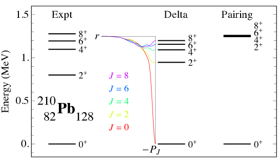
where $j$ is the orbital+spin angular momentum of a single nucleon (hence $j$ is half-odd-integer), $J$ results from the coupling of the angular momenta $j$ of the two nucleons and $M_{J}$ is the projection of $J$ on the $z$ axis. Furthermore, $g$ is the strength of the pairing interaction which is attractive in nuclei ($g>0$). Pairing is a reasonable, albeit schematic, approximation to the residual interaction between identical nucleons and hence can only be appropriate in semi-magic nuclei with valence nucleons of a single type, either neutrons or protons. The degree of approximation is illustrated in figure 1 for the nucleus ²¹⁰Pb which can be described as two neutrons in the $1g_{9/2}$ orbit outside the doubly magic ²⁰⁸Pb inert core. Also shown is the probability density $P_{J}$ to find two nucleons at a distance $r$ when they are in the $2g_{9/2}$ orbit of the harmonic oscillator and coupled to angular momentum $J$. This probability density at $r=0$ matches the energies of the zero-range delta interaction. The profiles of $P_{J}(r)$ for the different angular momenta show that any attractive short-range interaction favours the formation of a $J=0$ pair. This basic property of the nuclear force is accounted for by pairing.

Figure 1: The experimental low-energy spectrum of ²¹⁰Pb (left), and the corresponding spectra for a zero-range delta (middle) and for a pairing interaction (right). Levels are labelled by their angular momentum and parity $J^{\pi}$. The inset shows the probability density $P_{J}$ to find two nucleons at a distance $r$ when they are in the $2g_{9/2}$ orbit of a harmonic oscillator and coupled to angular momentum $J$.

The pairing interaction was introduced by Racah for the classification of electrons in an atom [4]. He was able to derive a closed formula for the interaction energy among the electrons and to prove that any eigenstate of the pairing interaction is characterized by a ‘seniority number’ $\upsilon$ which corresponds to the number of electrons that are not in pairs coupled to orbital angular momentum $L=0$. Racah’s original definition of seniority made use of coefficients of fractional parentage. He later noted that simplifications arose through the use of group theory [5]. Seniority turned out to be a label associated with the (unitary) symplectic algebra ${\rm Sp}(2j+1)$ in the classification

$$\begin{array}[]{ccccc}{\rm U}(2j+1)&\supset&{\rm Sp}(2j+1)&\supset&{\rm SU}(2)\\ \downarrow&&\downarrow&&\downarrow\\[0.0pt] [1^{n}]&&[1^{\upsilon}]&&J\end{array}.$$ (9)

Since the nucleons are identical, all states of the $j^{n}$ configuration belong to the totally anti-symmetric irreducible representation $[1^{n}]$ of ${\rm U}(2j+1)$. The irreducible representations of ${\rm Sp}(2j+1)$ therefore must also be totally anti-symmetric of the type $[1^{\upsilon}]$ with allowed values of seniority $\upsilon=n,n-2,\dots,1$ or 0.

In the definition (9) seniority appears as a label associated with the algebra ${\rm Sp}(2j+1)$. This has the drawback that, depending on $j$, the algebra can be quite large. Matters become even more complicated when the nucleons are non-identical and have isospin $t={\frac{1}{2}}$. The total number of single-particle states is then $\Omega\equiv(2j+1)(2t+1)$ and one quickly runs into formidable group-theoretical reduction problems. Fortunately, an alternative and simpler definition of seniority can be given in terms of algebras that do not change with $j$. The idea was simultaneously and independently proposed by Kerman [6] for $t=0$ (i.e., for identical nucleons) and by Helmers [7] for general $t$. It starts from operators $\hat{S}^{j}_{+}$ and $\hat{S}^{j}_{-}$ that create and annihilate pairs of particles in a single-$j$ shell and the commutator of which leads to a third kind of generator, $\hat{S}^{j}_{z}$, with one particle creation and one particle annihilation operator. This set of operators, known as quasi-spin operators, closes under commutation and forms the (unitary) symplectic algebra ${\rm Sp}(4t+2)$ which can be shown to have equivalent properties to those of ${\rm Sp}(2j+1)$, introduced in the classification (9).

The quasi-spin formulation of the pairing problem relies on the fact that the pairing interaction is related to the quadratic Casimir operator of the algebra ${\rm Sp}(4t+2)$. This allows a succinct and simultaneous derivation of the eigenvalues in the cases of identical nucleons ($t=0$) and of neutrons and protons ($t={\frac{1}{2}}$). Over the years many results have been derived and many extensions have been considered in both cases, which are discussed separately in the following.

3.1.1 Identical nucleons.

For $t=0$ one obtains the algebra Sp(2) which is isomorphic to SU(2). Due to its formal analogy with the spin algebra, the name ‘quasi-spin’ was coined by Kerman [6], and this terminology has stuck for all cases, even when $t\neq 0$.

The quasi-spin algebra ${\rm Sp}(2)\sim{\rm SU}(2)$ is obtained by noting that, in second quantization, the pairing interaction defined in equation (8) is written as

$$\hat{V}_{\rm pairing}=-g\hat{S}^{j}_{+}\hat{S}^{j}_{-},$$ (10)

with

$$\hat{S}^{j}_{+}={\frac{1}{2}}\sqrt{2j+1}\,(a_{j}^{\dagger}\times a_{j}^{\dagger})^{(0)}_{0},\qquad\hat{S}^{j}_{-}=\left(\hat{S}^{j}_{+}\right)^{\dagger},$$ (11)

where $a_{jm_{j}}^{\dagger}$ creates a nucleon in orbit $j$ with projection $m_{j}$. No isospin labels $t$ and $m_{t}$ are needed to characterize the identical nucleons. The symbol $\times$ refers to coupling in angular momentum and $\hat{S}^{j}_{+}$ therefore creates a pair of nucleons coupled to angular momentum $J=0$. The commutator $[\hat{S}^{j}_{+},\hat{S}^{j}_{-}]\equiv 2\hat{S}^{j}_{z}$, together with $[\hat{S}^{j}_{z},\hat{S}^{j}_{\pm}]=\pm\hat{S}^{j}_{\pm}$, shows that $\hat{S}^{j}_{+}$, $\hat{S}^{j}_{-}$ and $\hat{S}^{j}_{z}$ form a closed algebra SU(2).

Several emblematic results can be derived on the basis of SU(2). The quasi-spin symmetry allows the determination of the complete eigenspectrum of the pairing interaction which is given by

$$\hat{V}_{\rm pairing}|j^{n}\upsilon JM_{J}\rangle=E(n,\upsilon)|j^{n}\upsilon JM_{J}\rangle,$$ (12)

with

$$E(n,\upsilon)=-{\frac{g}{4}}(n-\upsilon)(2j-n-\upsilon+3).$$ (13)

Besides the nucleon number $n$, the total angular momentum $J$ and its projection $M_{J}$, all eigenstates are characterized by a seniority quantum number $\upsilon$ which counts the number of nucleons not in pairs coupled to angular momentum zero. For an attractive pairing interaction ($g>0$), the eigenstate with lowest energy has seniority $v=0$ if the nucleon number $n$ is even and $v=1$ if $n$ is odd. These lowest-energy eigenstates can, up to a normalization factor, be written as $(\hat{S}^{j}_{+})^{n/2}|{\rm o}\rangle$ for even $n$ and $a_{jm_{j}}^{\dagger}(\hat{S}^{j}_{+})^{n/2}|{\rm o}\rangle$ for odd $n$, where $|{\rm o}\rangle$ is the vacuum state for the nucleons.

The discussion of pairing correlations in nuclei traditionally has been inspired by the treatment of superfluidity in condensed matter, explained in 1957 by Bardeen, Cooper and Schrieffer [8], and later adapted to the discussion of pairing in nuclei [9]. The superfluid phase is characterized by the presence of a large number of identical bosons in a single quantum state. In superconductors the bosons are pairs of electrons with opposite momenta that form at the Fermi surface while in nuclei, according to the preceding discussion, they are pairs of valence nucleons with opposite angular momenta.

A generalization of these concepts concerns that towards several orbits. In case of degenerate orbits this can be achieved by making the substitution $\hat{S}^{j}_{\mu}\mapsto\hat{S}_{\mu}\equiv\sum_{j}\hat{S}^{j}_{\mu}$ which leaves all preceding results, valid for a single-$j$ shell, unchanged. The ensuing formalism can then be applied to semi-magic nuclei but, since it requires the assumption of a pairing interaction with degenerate orbits, its applicability is limited.

Figure 2: Graphical solution of the Richardson equation for two nucleons distributed over five single-particle orbits. The sum $\sum_{j}\Omega_{j}/(2\epsilon_{j}-E)\equiv y(E)$ (in MeV^-1) is plotted as a function of $E$ (in MeV). The intersections (red dots) of this curve (blue) with the (red) line $y=1/g$ correspond to the solutions of the Richardson equation.

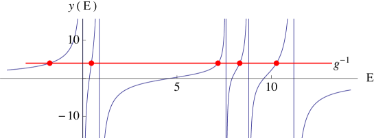
An exact method to solve the problem of particles distributed over non-degenerate levels interacting through a pairing force was proposed by Richardson [10] based on the Bethe ansatz and has been generalized more recently to other classes of integrable pairing models [11]. Richardson’s approach can be illustrated by supplementing the pairing interaction (10) with non-degenerate single-particle energies, to obtain the following hamiltonian:

$$\hat{H}_{\rm pairing}=\sum_{j}\epsilon_{j}\hat{n}_{j}-g\hat{S}_{+}\hat{S}_{-},$$ (14)

where $\hat{n}_{j}$ is the number operator for orbit $j$, $\epsilon_{j}$ is the single-particle energy of that orbit and $\hat{S}_{\pm}=\sum_{j}\hat{S}^{j}_{\pm}$. The solvability of the hamiltonian (14) arises as a result of the symmetry ${\rm SU}(2)\otimes{\rm SU}(2)\otimes\cdots$ where each SU(2) algebra pertains to a specific $j$. The eigenstates are of the form

$$\prod_{p=1}^{n/2}\left(\sum_{j}{\frac{\hat{S}^{j}_{+}}{2\epsilon_{j}-E_{p}}}\right)|{\rm o}\rangle,$$ (15)

where the $E_{p}$ are solutions of $n/2$ coupled, non-linear Richardson equations [10]

$$\sum_{j}{\frac{\Omega_{j}}{2\epsilon_{j}-E_{p}}}-\sum_{p^{\prime}(\neq p)}^{n/2}{\frac{2}{E_{p^{\prime}}-E_{p}}}={\frac{1}{g}},\qquad p=1,\dots,n/2,$$ (16)

with $\Omega_{j}=j+1/2$. This equation is solved graphically for the simple case of $n=2$ in figure 2. Each pair in the product (15) is defined through coefficients $\alpha_{j}=(2\epsilon_{j}-E_{p})^{-1}$ which depend on the energy $E_{p}$ where $p$ labels the $n/2$ pairs. A characteristic feature of the Bethe ansatz is that it no longer consists of a superposition of identical pairs since the coefficients $(2\epsilon_{j}-E_{p})^{-1}$ vary as $p$ runs from 1 to $n/2$. Richardson’s model thus provides a solution that covers all possible hamiltonians (14), ranging from those with superfluid character to those with little or no pairing correlations. Whether the solution can be called superfluid depends on the differences $\epsilon_{j}-\epsilon_{j^{\prime}}$ in relation to the strength $g$.

The pairing hamiltonian (14) admits non-degenerate single-particle orbits $\epsilon_{j}$ but requires a constant strength $g$ of the pairing interaction, independent of $j$. Alternatively, a hamiltonian with degenerate single-particle orbits $\epsilon_{j}=\epsilon$ but orbit-dependent strengths $g_{j}$,

$$\hat{H}^{\prime}_{\rm pairing}=\epsilon\sum_{j}\hat{n}_{j}-\sum_{j}g_{j}\hat{S}^{j}_{+}\sum_{j^{\prime}}g_{j^{\prime}}\hat{S}^{j^{\prime}}_{-},$$ (17)

can also be solved exactly based on the Bethe ansatz [12]. No exact solution is known, however, of a pairing hamiltonian with non-degenerate single-particle orbits $\epsilon_{j}$ and orbit-dependent strengths $g_{j}$, except in the case of two orbits [13]. Solvability by Richardson’s technique requires the pairing interaction to be separable with strengths that satisfy $g_{jj^{\prime}}=g_{j}g_{j^{\prime}}$ and no exact solution is known in the non-separable case when $g_{jj^{\prime}}\neq g_{j}g_{j^{\prime}}$.

These possible generalizations notwithstanding, it should be kept in mind that a pairing interaction is but an approximation to a realistic residual interaction among nucleons, as is clear from figure 1. A more generally valid approach is obtained if one imposes the following condition on the shell-model hamiltonian (7):

$$[[\hat{H}_{\rm GS},\hat{S}^{\alpha}_{+}],\hat{S}^{\alpha}_{+}]=\Delta\left(\hat{S}^{\alpha}_{+}\right)^{2},$$ (18)

where $\Delta$ is a constant and $\hat{S}^{\alpha}_{+}=\sum_{j}\alpha_{j}S^{j}_{+}$ creates the lowest two-particle eigenstate of $\hat{H}_{\rm GS}$ with energy $E_{0}$, $\hat{H}_{\rm GS}\hat{S}^{\alpha}_{+}|{\rm o}\rangle=E_{0}\hat{S}^{\alpha}_{+}|{\rm o}\rangle$. The condition (18) of generalized seniority, proposed by Talmi [14], is much weaker than the assumption of a pairing interaction and it does not require that the commutator $[\hat{S}^{\alpha}_{+},\hat{S}^{\alpha}_{-}]$ yields (up to a constant) the number operator which is central to the quasi-spin formalism. In spite of the absence of a closed algebraic structure, it is still possible to compute exact results for hamiltonians satisfying the condition (18). For an even number of nucleons, its ground state has the same simple structure as in the quasi-spin formalism,

$$\hat{H}_{\rm GS}\left(\hat{S}^{\alpha}_{+}\right)^{n/2}|{\rm o}\rangle=E_{\rm GS}(n)\left(\hat{S}^{\alpha}_{+}\right)^{n/2}|{\rm o}\rangle,$$

with an energy that can be computed for any nucleon number $n$,

$$E_{\rm GS}(n)=nE_{0}+{\frac{1}{2}}n(n-1)\Delta.$$

Because of its linear and quadratic dependence on the nucleon number $n$, this result can be considered as a generalization of Racah’s seniority formula (13), to which it reduces if $E_{0}=-g(j+1)/2$ and $\Delta=g/2$.

3.1.2 Neutrons and protons.

For $t={\frac{1}{2}}$ one obtains the quasi-spin algebra Sp(4) which is isomorphic to SO(5). The algebra ${\rm Sp}(4)$ or ${\rm SO}(5)$ is characterized by two labels, corresponding to seniority $\upsilon$ and reduced isospin $T_{\upsilon}$. Seniority $\upsilon$ has the same interpretation as in the like-nucleon case, namely the number of nucleons not in pairs coupled to angular momentum $J=0$, while reduced isospin $T_{\upsilon}$ corresponds to the total isospin of these nucleons [15, 16].

The above results are obtained from the general analysis as carried out by Helmers [7] for any $t$. It is of interest to carry out the analysis explicitly for the choice which applies to nuclei, namely $t={\frac{1}{2}}$. Results are given in $LS$ coupling, which turns out to be the more convenient scheme for the generalization to neutrons and protons.

Figure 3: Schematic illustration of the different types of nucleon pairs with orbital angular momentum $L=0$. The valence neutrons (blue) or protons (red) that form the pair occupy time-reversed orbits (circling the nucleus in opposite direction). If the nucleons are identical they must have anti-parallel spins—a configuration which is also allowed for a neutron–proton pair (top). The configuration with parallel spins is only allowed for a neutron–proton pair (bottom). Taken from reference [117].

If the $\ell$ shell contains neutrons and protons, the pairing interaction is assumed to be isospin invariant, which implies that it is the same in the three possible $T=1$ channels, neutron–neutron, neutron–proton and proton–proton, and that the pairing interaction (10) takes the form

$$\hat{V}^{\prime}_{\rm pairing}=-g\sum_{\mu}\hat{S}^{\ell}_{+,\mu}\hat{S}^{\ell}_{-,\mu}\equiv-g\hat{S}^{\ell}_{+}\cdot\hat{S}^{\ell}_{-},$$ (19)

where the dot indicates a scalar product in isospin. In terms of the nucleon operators $a^{\dagger}_{\ell m_{\ell},sm_{s},tm_{t}}$, which now carry also isospin indices (with $t={\frac{1}{2}}$), the pair operators are

$$\hat{S}^{\ell}_{+,\mu}=\sqrt{\frac{1}{2}}\sqrt{2\ell+1}(a_{\ell,s,t}^{\dagger}\times a_{\ell,s,t}^{\dagger})^{(001)}_{00\mu},\qquad\hat{S}^{\ell}_{-,\mu}=\left(\hat{S}^{\ell}_{+,\mu}\right)^{\dagger},$$ (20)

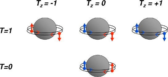
where $\hat{S}$ refers to a pair with orbital angular momentum $L=0$, spin $S=0$ and isospin $T=1$. The index $\mu$ (isospin projection) distinguishes neutron–neutron ($\mu=+1$), neutron–proton ($\mu=0$) and proton–proton ($\mu=-1$) pairs. There are thus three different pairs with $L=0$, $S=0$ and $T=1$ (top line in figure 3) and they are related through the action of the isospin raising and lowering operators $\hat{T}_{\pm}$. The quasi-spin algebra associated with the hamiltonian (19) is SO(5) and makes the problem analytically solvable [17].

For a neutron and a proton there exists a different paired state with parallel spins (bottom line of figure 3). The most general pairing interaction for a system of neutrons and protons is therefore

$$\hat{V}^{\prime\prime}_{\rm pairing}=-g\hat{S}^{\ell}_{+}\cdot\hat{S}^{\ell}_{-}-g^{\prime}\hat{P}^{\ell}_{+}\cdot\hat{P}^{\ell}_{-},$$ (21)

where $\hat{P}$ refers to a pair with orbital angular momentum $L=0$, spin $S=1$ and isospin $T=0$,

$$\hat{P}^{\ell}_{+,\mu}=\sqrt{\frac{1}{2}}\sqrt{2\ell+1}(a_{\ell,s,t}^{\dagger}\times a_{\ell,s,t}^{\dagger})^{(010)}_{0\mu 0},\qquad\hat{P}^{\ell}_{-,\mu}=\left(\hat{P}^{\ell}_{+,\mu}\right)^{\dagger}.$$ (22)

The index $\mu$ is the spin projection and distinguishes the three spatial orientations of the $S=1$ pair. The pairing interaction (21) now involves two parameters $g$ and $g^{\prime}$, the strengths of the isovector and isoscalar components. Solutions with an intrinsically different structure are obtained for different ratios $g/g^{\prime}$.

In general, the eigenproblem associated with the pairing interaction (21) can only be solved numerically which, given a typical size of a shell-model space, can be a formidable task. However, for specific choices of $g$ and $g^{\prime}$ the solution of $\hat{V}^{\prime\prime}_{\rm pairing}$ can be obtained analytically [18, 19]. The analysis reveals the existence of a quasi-spin algebra SO(8) formed by the pair operators (20) and (22), their commutators, the commutators of these among themselves, and so on until a closed algebraic structure is attained. Closure is obtained by introducing, in addition to the pair operators (20) and (22), the number operator $\hat{n}$, the spin and isospin operators $\hat{S}_{\mu}$ and $\hat{T}_{\mu}$, and the Gamow-Teller-like operators $\hat{U}_{\mu\nu}$, defined in section 3.2 in the context of Wigner’s supermultiplet algebra.

From a study of the subalgebras of SO(8) it can be concluded that the pairing interaction (21) has a dynamical symmetry (in the sense of section 2) in one of the three following cases: (i) $g=0$, (ii) $g^{\prime}=0$ and (iii) $g=g^{\prime}$, corresponding to pure isoscalar pairing, pure isovector pairing and pairing with equal isoscalar and isovector strengths, respectively. Seniority $\upsilon$ turns out to be conserved in these three limits and associated with either an SO(5) algebra in cases (i) and (ii), or with the SO(8) algebra in case (iii).

One of the main results of the theory of pairing between identical nucleons is the recognition of the special structure of low-energy states in terms of $S$ pairs. It is therefore of interest to address the same question in the theory of pairing between neutrons and protons. The nature of SO(8) superfluidity can be illustrated with the example of the ground state of nuclei with an equal number of neutrons $N$ and protons $Z$. For equal strengths of isoscalar and isovector pairing, $g=g^{\prime}$, the pairing interaction (21) is solvable and its ground state can be shown to be [20]:

$$\left(\hat{S}^{\ell}_{+}\cdot\hat{S}^{\ell}_{+}-\hat{P}^{\ell}_{+}\cdot\hat{P}^{\ell}_{+}\right)^{n/4}|{\rm o}\rangle.$$ (23)

This shows that the superfluid solution acquires a quartet structure in the sense that it reduces to a condensate of a boson-like object, which corresponds to four nucleons. Since this object in (23) is scalar in spin and isospin, it can be thought of as an $\alpha$ particle; its orbital character, however, might be different from that of an actual $\alpha$ particle. A quartet structure is also present in the other two limits of SO(8), with either $g=0$ or $g^{\prime}=0$, which have a ground-state wave function of the type (23) with either the first or the second term suppressed. Thus, a reasonable ansatz for the ground-state wave function of an $N=Z$ nucleus of the pairing interaction (21) with arbitrary strengths $g$ and $g^{\prime}$ is

$$\left(\cos\theta\;\hat{S}^{\ell}_{+}\cdot\hat{S}^{\ell}_{+}-\sin\theta\;\hat{P}^{\ell}_{+}\cdot\hat{P}^{\ell}_{+}\right)^{n/4}|{\rm o}\rangle,$$ (24)

where $\theta$ is a parameter that depends on the ratio $g/g^{\prime}$.

The condensate (24) of $\alpha$-like particles can serve as a good approximation to the $N=Z$ ground state of the pairing interaction (21) for any combination of $g$ and $g^{\prime}$ [20]. Nevertheless, it should be stressed that, in the presence of both neutrons and protons in the valence shell, the pairing interaction (21) is not a good approximation to a realistic shell-model hamiltonian which contains an important quadrupole component (see, e.g., the shell-model review [3]). Consequently, any model based on $L=0$ fermion pairs only, remains necessarily schematic in nature. A realistic model should include also $L\neq 0$ pairs.

3.2 Wigner’s supermultiplet model

Wigner’s supermultiplet model [21] assumes nuclear forces to be invariant under rotations in spin as well as isospin space. A shell-model hamiltonian with this property satifies the following commutation relations:

$$[\hat{H},\hat{S}_{\mu}]=[\hat{H},\hat{T}_{\mu}]=[\hat{H},\hat{U}_{\mu\nu}]=0,$$ (25)

where

$$\hat{S}_{\mu}=\sum_{k=1}^{A}\hat{s}_{k,\mu},\qquad\hat{T}_{\mu}=\sum_{k=1}^{A}\hat{t}_{k,\mu},\qquad\hat{U}_{\mu\nu}=\sum_{k=1}^{A}\hat{s}_{k,\mu}\hat{t}_{k,\nu},$$ (26)

are the spin, isospin and spin–isospin operators, in terms of $\hat{s}_{k,\mu}$ and $\hat{t}_{k,\mu}$, the spin and isospin components of nucleon $k$. The 15 operators (26) generate the Lie algebra SU(4). According to the discussion in section 2, any hamiltonian satisfying the conditions (25) has SU(4) symmetry, and this in addition to symmetries associated with the conservation of total spin $S$ and total isospin $T$.

The physical relevance of Wigner’s supermultiplet classification is due to the short-range attractive nature of the residual interaction as a result of which states with spatial symmetry are favoured energetically. To obtain a qualitative understanding of SU(4) symmetry, it is instructive to analyze the case of two nucleons. Total anti-symmetry of the wave function requires that the spatial part is symmetric and the spin-isospin part anti-symmetric or vice versa. Both cases correspond to a different symmetry under SU(4), the first being anti-symmetric and the second symmetric. The symmetry under a given algebra can characterized by the so-called Young tableau [108]. For two nucleons the symmetric and anti-symmetric irreducible representations are denoted by

$$\Box\Box\equiv[2,0],\qquad\begin{array}[]{c}\Box\\[-4.30554pt] \Box\end{array}\equiv[1,1],$$

respectively, and the Young tableaux are conjugate, that is, one is obtained from the other by interchanging rows and columns. This result can be generalized to many nucleons, leading to the conclusion that the energy of a state depends on its SU(4) labels, which are three in number and denoted here as $(\bar{\lambda},\bar{\mu},\bar{\nu})$.

Wigner’s supermultiplet model is an $LS$-coupling scheme which is not appropriate for nuclei. In spite of its limited applicability, Wigner’s idea remains important because it demonstrates the connection between the short-range character of the residual interaction and the spatial symmetry of the many-body wave function. The break down of SU(4) symmetry is a consequence of the spin–orbit term in the shell-model hamiltonian (7) which does not satisfy the first and third commutator in equation (25). The spin–orbit term breaks SU(4) symmetry [SU(4) irreducible representations are admixed by it] and does so increasingly in heavier nuclei since the energy splitting of the spin doublets $\ell-{\frac{1}{2}}$ and $\ell+{\frac{1}{2}}$ increases with nucleon number $A$. In addition, SU(4) symmetry is also broken by the Coulomb interaction—an effect that also increases with $A$—and by spin-dependent residual interactions.

3.3 Elliott’s rotation model

In Wigner’s supermultiplet model the spatial part of the wave function is characterized by a total orbital angular momentum $L$ but is left unspecified otherwise. The main feature of Elliott’s model [22] is that it provides additional orbital quantum numbers that are relevant for deformed nuclei. Elliott’s model of rotation presupposes Wigner’s SU(4) classification and assumes in addition that the residual interaction has a quadrupole character which is a reasonable hypothesis if the valence shell contains neutrons and protons. One requires that the schematic shell-model hamiltonian (7) reduces to

$$\hat{H}_{\rm SU(3)}=\sum_{k=1}^{A}\left({\frac{\hat{p}_{k}^{2}}{2m_{k}}}+{\frac{1}{2}}m_{k}\omega^{2}r_{k}^{2}\right)+\hat{V}_{\rm quadrupole},$$ (27)

where $\hat{V}_{\rm quadrupole}=-g_{2}\hat{Q}\cdot\hat{Q}$ contains a quadrupole operator

$$\hat{Q}_{\mu}=\sqrt{\frac{3}{2}}\left[\sum_{k=1}^{A}\frac{1}{b^{2}}(\bar{r}_{k}\wedge\bar{r}_{k})^{(2)}_{\mu}+\frac{b^{2}}{\hbar^{2}}\sum_{k=1}^{A}(\bar{p}_{k}\wedge\bar{p}_{k})^{(2)}_{\mu}\right],$$ (28)

in terms of coordinates $\bar{r}_{k}$ and momenta $\bar{p}_{k}$ of nucleon $k$, and where $b$ is the oscillator length parameter, $b=\sqrt{\hbar/m_{\rm n}\omega}$ with $m_{\rm n}$ the mass of the nucleon.

With use of the techniques explained in section 2, it can be shown that the shell-model hamiltonian (27) is analytically solvable. Since the hamiltonian (27) satisfies the commutation relations (25), it has SU(4) symmetry and its eigenstates are characterized by the associated quantum numbers, the supermultiplet labels $(\bar{\lambda},\bar{\mu},\bar{\nu})$. The spin–isospin symmetry SU(4) is equivalent through conjugation to the orbital symmetry ${\rm U}(\Omega)$, where $\Omega$ denotes the orbital shell size (i.e., $\Omega=1,3,6,\dots$ for the $s$, $p$, $sd$,…shells). The algebra ${\rm U}(\Omega)$, however, is not a true symmetry of the hamiltonian (27) but is broken according to the nested chain of algebras ${\rm U}(\Omega)\supset{\rm SU}(3)\supset{\rm SO}(3)$. As a result one finds that the hamiltonian (27) has the eigenstates $|[1^{n}](\bar{\lambda},\bar{\mu},\bar{\nu})(\lambda,\mu)K_{L}LM_{L}SM_{S}TM_{T}\rangle$ with energies

$$E_{\rm SU(3)}(\lambda,\mu,L)=E_{0}-g_{2}\left[4(\lambda^{2}+\mu^{2}+\lambda\mu+3\lambda+3\mu)-3L(L+1)\right],$$

where $E_{0}$ is a constant energy associated with the first term in the hamiltonian (27). Besides the set of quantum numbers encountered in Wigner’s supermultiplet model, that is, the SU(4) labels $(\bar{\lambda},\bar{\mu},\bar{\nu})$, the total orbital angular momentum $L$ and its projection $M_{L}$, the total spin $S$ and its projection $M_{S}$, and the total isospin $T$ and its projection $M_{T}$, all eigenstates of the hamiltonian (27) are characterized by the SU(3) quantum numbers $(\lambda,\mu)$ and an additional label $K_{L}$. Each irreducible representation $(\lambda,\mu)$ contains the orbital angular momenta $L$ typical of a rotational band, cut off at some upper limit [22]. The label $K_{L}$ defines the intrinsic state associated to that band and can be interpreted as the projection of the orbital angular momentum $L$ on the axis of symmetry of the rotating deformed nucleus.

The importance of Elliott’s idea is that it gives rise to a rotational classification of states through mixing of spherical configurations. With the SU(3) model it was shown, for the first time, how deformed nuclear shapes may arise out of the spherical shell model. As a consequence, Elliott’s work bridged the gap between the spherical nuclear shell model and the geometric collective model (see section 4) which up to that time (1958) existed as separate views of the nucleus.

Figure 4: The single-particle energies (for a non-zero quadratic orbital strength, $\zeta_{\ell\ell}\neq 0$) in SU(3), quasi-SU(3) and pseudo-SU(3) for the example of the $sdg$ oscillator shell. The spin–orbit strength is $\zeta_{\ell s}\approx 0$ in SU(3), $\zeta_{\ell s}\approx 2\zeta_{\ell\ell}$ in quasi-SU(3) and $\zeta_{\ell s}\approx 4\zeta_{\ell\ell}$ in pseudo-SU(3). The single-particle spaces in red and in blue are assumed to be approximately decoupled. In pseudo-SU(3) the level degeneracies can be interpreted in terms of a pseudo-spin symmetry.

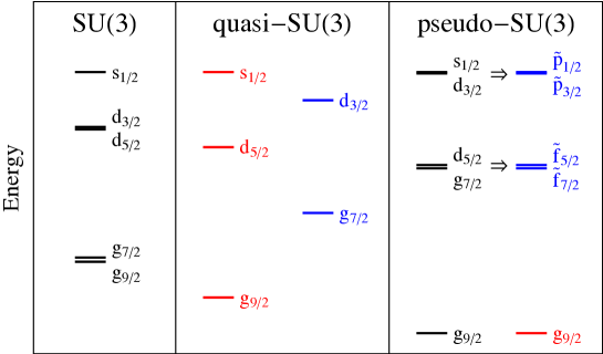
Elliott’s SU(3) model provides a natural explanation of rotational phenomena, ubiquitous in nuclei, but it does so by assuming Wigner’s SU(4) symmetry which is known to be badly broken in most nuclei. This puzzle has motivated much work since Elliott: How can rotational phenomena in nuclei be understood starting from a $jj$-coupling scheme which applies to most nuclei? Over the years several schemes have been proposed with the aim of transposing the SU(3) scheme to those modified situations. One such modification has been suggested by Zuker et al. [23] under the name of quasi-SU(3) and it invokes the similarities of matrix elements of the quadrupole operator in the $jj$- and $LS$-coupling schemes.

Arguably the most successful way to extend the applications of the SU(3) model to heavy nuclei is based upon the concept of pseudo-spin symmetry. The starting point for the explanation of this symmetry is the single-particle part of the hamiltonian (7). For $\zeta_{\ell\ell}=\zeta_{\ell s}=0$ a three-dimensional isotropic harmonic oscillator is obtained which exhibits degeneracies associated with U(3) symmetry. For arbitrary non-zero values of $\zeta_{\ell\ell}$ and $\zeta_{\ell s}$ this symmetry is broken. However, for the particular combination $4\zeta_{\ell\ell}=\zeta_{\ell s}$ some degree of degeneracy, associated with a so-called pseudo-spin symmetry, is restored in the single-particle spectrum (see figure 4).

Pseudo-spin symmetry has a long history in nuclear physics. The existence of nearly degenerate pseudo-spin doublets in the nuclear mean-field potential was pointed out almost forty years ago by Hecht and Adler [24] and by Arima et al. [25] who noted that, because of the small pseudo-spin–orbit splitting, pseudo-$LS$ coupling should be a reasonable starting point in medium-mass and heavy nuclei where $LS$ coupling becomes unacceptable. With pseudo-$LS$ coupling as a premise, a pseudo-SU(3) model can be constructed [26] in much the same way as Elliott’s SU(3) model can be defined in $LS$ coupling. It is only many years after its original suggestion that Ginocchio showed pseudo-spin to be a symmetry of the Dirac equation which occurs if the scalar and vector potentials are equal in size but opposite in sign [27].

The models discussed so far all share the property of being confined to a single shell, either an oscillator or a pseudo-oscillator shell. A full description of nuclear collective motion requires correlations that involve configurations outside a single (pseudo) oscillator shell. The proper framework for such correlations invokes the concept of a non-compact algebra which, in contrast to a compact one, can have infinite-dimensional unitary irreducible representations. The latter condition is necessary since the excitations into higher shells can be infinite in number. The inclusion of excitations into higher shells of the harmonic oscillator, was achieved by Rosensteel and Rowe by embedding the SU(3) algebra into the (non-compact) symplectic algebra Sp(3,R) [28].

3.4 The Lipkin model

Another noteworthy algebraic model in nuclear physics is due to Lipkin et al. [29] who consider two levels (assigned an index $\sigma=\pm$) each with degeneracy $\Omega$ over which $n$ fermions are distributed. The Lipkin model has an SU(2) algebraic structure which is generated by the operators

$$\hat{K}_{+}=\sum_{m}a^{\dagger}_{m+}a_{m-},\qquad\hat{K}_{-}=\left(\hat{K}_{+}\right)^{\dagger},\qquad\hat{K}_{z}={\frac{1}{2}}(\hat{n}_{+}-\hat{n}_{-}),$$

written in terms of the creation and annihilation operators $a^{\dagger}_{m\sigma}$ and $a_{m\sigma}$, with $m=1,\dots,\Omega$ and $\sigma=\pm$, and where $\hat{n}_{\pm}$ counts the number of nucleons in the level with $\sigma=\pm$. The hamiltonian

$$\hat{H}=\epsilon\hat{K}_{z}+{\frac{1}{2}}\upsilon\left(\hat{K}_{+}\hat{K}_{-}+\hat{K}_{-}\hat{K}_{+}\right)+{\frac{1}{2}}\omega\left(\hat{K}_{+}^{2}+\hat{K}_{-}^{2}\right),$$

can, with use of the underlying SU(2) algebra, be solved analytically for certain values of the parameters $\epsilon$, $\upsilon$ and $\omega$. These have a simple physical meaning: $\epsilon$ is the energy needed to promote a nucleon from the lower level with $\sigma=-$ to the upper level with $\sigma=+$, $\upsilon$ is the strength of the interaction that mixes configurations with the same nucleon numbers $n_{-}$ and $n_{+}$, and $\omega$ is the strength of the interaction that mixes configurations differing by two in these numbers. The Lipkin model has thus three ingredients (albeit in schematic form) that are of importance in determining the structure of nuclei: an interaction $\upsilon$ between the nucleons in a valence shell, the possibility to excite nucleons from the valence shell into a higher shell at the cost of an energy $\epsilon$, and an interaction $\omega$ that mixes these particle–hole excitations with the valence configurations. With these ingredients the Lipkin model has played an important role as a testing ground of various approximations proposed in nuclear physics, examples of which are given in reference [112].

4 Geometric collective models

In 1879, in a study of the properties of a droplet of incompressible liquid, Lord Rayleigh showed [30] that its normal modes of vibration are described by the variables $\alpha_{\lambda\mu}$ which appear in the expansion of the droplet’s radius,

$$R(\theta,\phi)=R_{0}\left(1+\sum_{\lambda\mu}\alpha_{\lambda\mu}^{*}Y_{\lambda\mu}(\theta,\phi)\right),$$ (29)

where $Y_{\lambda\mu}(\theta,\phi)$ are spherical harmonics in terms of the spherical angles $\theta$ and $\phi$. Since the atomic nucleus from early on was modeled as a dense, charged liquid drop [31], it was natural for nuclear physicists to adopt the same multipole parameterization (29), as was done in the classical papers on the geometric collective model by Rainwater [32], Bohr [33], and Bohr and Mottelson [34].

As was also shown by Lord Rayleigh, the multipolarity that corresponds to the normal mode with lowest eigenfrequency is of quadrupole nature, $\lambda=2$. The quadrupole collective coordinates $\alpha_{2\mu}$ can be transformed to an intrinsic-axes system through $a_{2\mu}=\sum_{\nu}{\cal D}^{2}_{\nu\mu}(\theta_{i})\alpha_{2\nu}$, with ${\cal D}^{2}_{\nu\mu}(\theta_{i})$ the Wigner $\cal D$ functions in terms of the Euler angles $\theta_{i}$ that rotate the laboratory frame into the intrinsic frame. If the intrinsic frame is chosen to coincide with the principal axes of the quadrupole-deformed ellipsoid, the $a_{2\mu}$ satisfy $a_{2-1}=a_{2+1}=0$ and $a_{2-2}=a_{2+2}$ while the remaining two variables can be transformed further to two coordinates $\beta$ and $\gamma$, according to $a_{0}=\beta\cos\gamma$ and $a_{2-2}=a_{2+2}=\beta\sin\gamma/\sqrt{2}$. The coordinate $\beta\geq 0$ parameterizes deviations from sphericity while $\gamma$ is a polar coordinate confined to the interval $[0,\pi/3]$. For $\gamma=0$ the intrinsic shape is axially symmetric and prolate, for $\gamma=\pi/3$ it is axially symmetric and oblate, and intermediate values of $\gamma$ describe triaxial shapes.

The classical problem of quadrupole oscillations of a droplet has been quantized by Bohr [33], resulting in the hamiltonian

$$\hat{H}_{\rm B}=\hat{T}_{\beta}+\hat{T}_{\gamma}+\hat{T}_{\rm rot}+V(\beta,\gamma),$$

where $\hat{T}$ ($V$) refers to kinetic (potential) energy. The kinetic energy has three contributions coming from $\beta$ oscillations which preserve axial symmetry, from $\gamma$ oscillations which do not and from the rotation of a quadrupole-deformed object. Bohr’s analysis results in a collective Schrödinger equation $\hat{H}_{\rm B}\Psi(\beta,\gamma,\theta_{i})=E\Psi(\beta,\gamma,\theta_{i})$ with

$$\hat{H}_{\rm B} = -\frac{\hbar^{2}}{2B_{2}}\left[\frac{1}{\beta^{4}}\frac{\partial}{\partial\beta}\beta^{4}\frac{\partial}{\partial\beta}+\frac{1}{\beta^{2}\sin 3\gamma}\frac{\partial}{\partial\gamma}\sin 3\gamma\frac{\partial}{\partial\gamma}\right]$$ (30)

$$+\frac{\hbar^{2}}{8B_{2}}\sum_{k=1}^{3}\frac{\hat{L}_{k}^{\prime 2}}{\beta^{2}\sin^{2}(\gamma-2\pi k/3)},$$

where $B_{2}=\rho R_{0}^{5}/2$ is the mass parameter in terms of the constant matter density $\rho$ for an incompressible nucleus. The operators $\hat{L}_{k}^{\prime}$ are the components of the angular momentum in the intrinsic frame of reference where the prime is used to distinguish these from the components of the angular momentum in the laboratory frame of reference. The collective coordinates are coupled in an intricate way in the Bohr hamiltonian (30) and this limits the number of exactly solvable cases. In particular, because of the $\gamma$ dependence of the moments of inertia, $\gamma$ excitations are strongly coupled to the collective rotational motion. It turns out that $\beta$ excitations are less strongly coupled and a judicious choice of the potential may well lead to a separation of $\beta$ from the $\gamma$ and $\theta_{i}$ coordinates.

4.1 Exactly solvable collective models

A way to decouple the Bohr hamiltonian (30) into separate differential equations was proposed by Wilets and Jean [35] and requires a potential of the form

$$V(\beta,\gamma)=V_{1}(\beta)+\frac{V_{2}(\gamma)}{\beta^{2}},$$

leading to the coupled equations

$$\Bigg{[}-\frac{1}{\beta^{4}}\frac{\partial}{\partial\beta}\beta^{4}\frac{\partial}{\partial\beta}+u_{1}(\beta)-\varepsilon+\frac{\omega}{\beta^{2}}\Bigg{]}\xi(\beta)=0,$$ (31)

$$\Bigg{[}-\frac{1}{\sin 3\gamma}\frac{\partial}{\partial\gamma}\sin 3\gamma\frac{\partial}{\partial\gamma}+\sum_{k=1}^{3}\frac{\hat{L}^{\prime 2}_{k}}{4\sin^{2}(\gamma-2\pi k/3)}+u_{2}(\gamma)-\omega\Bigg{]}\psi(\gamma,\theta_{i})=0,$$

(32)

where $\omega$ is the separation constant, $\varepsilon=(2B_{2}/\hbar^{2})E$ and $u_{i}=(2B_{2}/\hbar^{2})V_{i}$ ($i=1,2$). The first equation can only be solved exactly if the constant $\omega$ is obtained from the solution of the second one. At present the only known analytic solution of the Bohr hamiltonian (30) is for $\gamma$-independent potentials [35], that is, for $V_{2}(\gamma)=0$. In that case, one still needs to determine the allowed values of $\omega$ in the equation (32). Many techniques have been proposed to solve this equation relying on either algebraic or analytic methods. Rakavy [36] noticed that the first two terms in equation (32) correspond to the Casimir operator of the orthogonal group in five dimensions, SO(5), and it is known from group-theoretical arguments that $\omega$ therefore acquires the values $\omega=v(v+3)$ with $v=1,2,\dots$, leading to the following equation in $\beta$:

$$\left[-\frac{1}{\beta^{4}}\frac{\partial}{\partial\beta}\beta^{4}\frac{\partial}{\partial\beta}+u_{1}(\beta)-\varepsilon+\frac{v(v+3)}{\beta^{2}}\right]\xi(\beta)=0.$$ (33)

Special choices of $u_{1}(\beta)$ [or $V_{1}(\beta)$] lead to the following exact solutions of the Bohr hamiltonian (30).

4.1.1 The five-dimensional harmonic oscillator.

The harmonic quadrupole oscillator was the first potential used in an exactly solvable collective model [33]. The potential $V(\beta,\gamma)$ reduces to a single term $V(\beta)=C_{2}\beta^{2}/2$ where $C_{2}$ is a constant. Even though one does not expect harmonic quadrupole vibrations to appear in the experimental study of atomic nuclei, the model serves as an interesting benchmark. The solution of the differential equation in $\beta$ results in the energy spectrum $E(n,v)=\hbar\Omega(2n+v+5/2)$ with $\Omega=\sqrt{C_{2}/B_{2}}$ and the corresponding eigenfunctions are associated Legendre polynomials of order $v+3/2$. The energy spectrum is characterized by degeneracies that increase with increasing $n$ and $v$. The complete solution of the Bohr hamiltonian with a harmonic potential can be obtained with group-theoretical methods based on the reduction ${\rm U}(5)\supset{\rm SO}(5)\supset{\rm SO}(3)$ [37]. An alternative derivation is based on the notion of quasi-spin discussed in subsection 3.1.1 which for bosons has the algebraic structure is SU(1,1) [38].

4.1.2 The infinite square-well potential.

It was shown by Wilets and Jean  [35] that the spectrum of the five-dimensional harmonic oscillator can be made anharmonic by introducing a potential in $\beta$ that has the form of an infinite square well, that is, $V(\beta)={\rm constant}$ for $\beta\leq b$ and $V(\beta)=\infty$ for $\beta>b$. This leads to solutions of equation (33) that are Bessel functions with allowed values for $v$ resulting from the boundary condition of a vanishing wave function at $\beta=b$.

The solution of this problem has been worked out much later by Iachello [39] in the context of a study on shape transitions from spherical and to $\gamma$-soft potentials. The spectrum is determined by the energy eigenvalues

$$E(i,v)=\frac{\hbar^{2}}{2B_{2}}k^{2}_{i,v},\qquad k_{i,v}=\frac{x_{i,v}}{b},$$

with corresponding eigenfunctions

$$\xi_{i,v}(\beta)\propto\beta^{-3/2}J_{v+3/2}(k_{i,v}\beta),$$

where $x_{i,v}$ is the $i$th zero of the Bessel function $J_{v+3/2}(x)$. This solution, referred to as E(5), proves therefore to be exact, as discussed in great detail in reference [39].

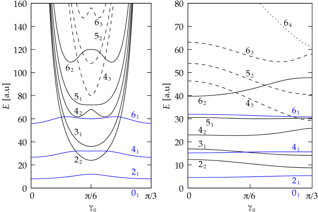
4.1.3 The Davidson potential.

The five-dimensional analogue of a three-dimensional potential, proposed by Davidson [40] for use in molecular physics, gives rise to another analytic solution of the Bohr hamiltonian. The constraint of $\gamma$ independence is kept and the harmonic potential of subsection 4.1.1 is modified to $V(\beta)=C_{2}(\beta^{2}+\beta_{0}^{4}/\beta^{2})/2$. The additional term changes the spherical potential into a deformed one with a minimum value located at $\beta_{0}$. The energy spectrum of the modified potential can be obtained from the spherical one after the substitution $v\mapsto\tilde{v}$, with $\tilde{v}$ defined from $\tilde{v}(\tilde{v}+3)=v(v+3)+k\beta_{0}^{4}$ with $k=B_{2}C_{2}/\hbar^{2}$. The resulting energy spectrum is shown in figure 5. The corresponding problem with a mass parameter $B_{2}$ depending on the coordinate $\beta$ has also been studied [41]. If one considers the form $B_{2}=B_{2}(0)/(1+a\beta^{2})^{2}$, the problem becomes exactly solvable with use of techniques from supersymmetric quantum mechanics [42] and by imposing integrability conditions, also called shape invariance [43].

Figure 5: The energy spectrum $E(n,\tilde{v})=2n+\tilde{v}+5/2$ (in units $\hbar\Omega$) of the Davidson potential as a function of the deformation parameter $\beta_{0}$. Taken from reference [55].

4.1.4 Other analytic solutions.

There are other $\gamma$-independent potentials $V(\beta)$ that lead to a solvable equation (33) and therefore yield an exactly solvable Bohr hamiltonian. Most notably, they are the Coulomb potential $V(\beta)=-A/\beta$ and the Kratzer potential $V(\beta)=-B[\beta_{0}/\beta-\beta^{2}_{0}/(2\beta^{2})]$ [44]. Also potentials of the form $V(\beta)=\beta^{2n}$ ($n=1,2,\dots$) have been studied, which for $n=1$ reduce to the five-dimensional harmonic oscillator and for $n\rightarrow\infty$ approach the infinite square-well potential, but with numerical techniques (see, e.g., the reviews [45, 46]). Lévai and Arias [47] proposed a sextic potential leading to a quasi-exactly solvable model [48, 49] which reduces to a class of two-parameter potentials containing terms in $\beta^{2}$, $\beta^{4}$ and $\beta^{6}$. This choice leads to exact solutions of the Bohr hamiltonian for a finite subset of states, here in particular for the lowest few eigenstates (energies, wave functions and a subset of $B$(E2) values). Finally, the particular choice $V(\beta)=C_{2}b\beta^{2}/(1+b\beta^{2})$, proposed by Ginocchio [50], is solvable. It leads to a solution of the Bohr hamiltonian that reproduces the lowest energy eigenvalues of an anharmonic vibrator [or of the U(5) limit of the IBM, see section 5].

4.2 Triaxial models

Many nuclei may exhibit excursions away from axial symmetry, requiring the introduction of explicit triaxial features in the Bohr hamiltonian. Due to the coupling of vibrational and rotational degrees of freedom in the Bohr hamiltonian, potentials with $\gamma$ dependence allow very few exact solutions, even if they are of the separable type, $V(\beta,\gamma)=V_{1}(\beta)+V_{2}(\gamma)$. In early attempts to address this more complicated situation, triaxial rotors were studied in an adiabatic approximation which implies that the nucleus’ intrinsic shape does not change under the effect of rotation. Such systems, in the context of the Bohr hamiltonian, correspond to a potential of the type $V(\beta,\gamma)=\delta(\beta-\beta_{0})\delta(\gamma-\gamma_{0})$ and their hamiltonian contains a rotational kinetic energy term only. On the other hand, the quantum mechanics of a rotating rigid body was studied much before the advent of the Bohr hamiltonian, by Reiche [51] and by Casimir [52], starting from a classical description of rotating bodies. The two approaches give rise to rather different moments of inertia, as discussed in the next subsection 4.2.1.

4.2.1 Rigid rotor models.

Davydov and co-workers [53, 54] studied and solved a triaxial rotor model in the context of the Bohr hamiltonian, which in the adiabatic approximation reduces to its rotational part,

$$\hat{H}_{\rm rot}=\frac{\hbar^{2}}{8B_{2}}\sum_{k=1}^{3}\frac{\hat{L}_{k}^{\prime 2}}{\beta_{0}^{2}\sin^{2}(\gamma_{0}-2\pi k/3)},$$ (34)

where $\beta_{0}$ and $\gamma_{0}$ are fixed values that define the shape of the rotating nucleus. The dependence of the moments of inertia ${\cal J}_{k}=4B_{2}\beta_{0}^{2}\sin^{2}(\gamma_{0}-2\pi k/3)$ on the shape parameters $\beta_{0}$ and $\gamma_{0}$ is that of a droplet in irrotational flow, that is, of which the velocity field $\bar{v}(\bar{r})$ obeys the condition $\bar{\nabla}\wedge\bar{v}(\bar{r})=0$.

The Davydov model is exactly solvable in the sense that the energies of the lowest-spin states $L^{\pi}=0^{+},2^{+},3^{+},\dots$ can be derived in closed form. For higher-spin states the energies are obtained as solutions of higher-order algebraic equations: cubic for $L^{\pi}=4^{+}$, quartic for $L^{\pi}=6^{+}$, etc. The corresponding wave functions only depend on the Euler angles $\theta_{i}$ and can be expressed as $\Phi_{iLM}(\theta_{i})=\sum_{K}a_{K}^{i}\Phi_{KLM}(\theta_{i})$, with coefficients $a_{K}^{i}$ obtained from the same algebraic equations, and

$$\Phi_{KLM}(\theta_{i})=\sqrt{\frac{2L+1}{16\pi^{2}(1+\delta_{K0})}}\left[{\cal D}_{MK}^{L}(\theta_{i})+(-)^{L}{\cal D}_{M,-K}^{L}(\theta_{i})\right],$$

where ${\cal D}_{MK}^{L}(\theta_{i})$ are the Wigner $\cal D$ functions. These expressions also allow the calculation of electromagnetic transitions [53].

Figure 6: The energy spectrum of a rigid rotor, with irrotational (left) and rigid (right) values for the moments of inertia and with energy in units $\hbar^{2}/(8B_{2})$ and $5\hbar^{2}/(4m_{\rm n}AR_{0}^{2})$, respectively. In both cases $\beta_{0}=1$. Taken from reference [55].

The classical expressions for the moments of inertia of a rigid body with quadrupole deformation, on the other hand, are ${\cal J}_{k}=(2m_{\rm n}AR_{0}^{2}/5)[1-\sqrt{5/4\pi}\beta_{0}\cos(\gamma_{0}-2\pi k/3)]$ where $m_{\rm n}A$ is the mass. As a result, its quantum-mechanical rotation leads to an energy spectrum [51, 52] which is different from the one obtained with the Bohr hamiltonian (see figure 6). The most obvious difference between the two cases occurs in the limits of axial symmetry ($\gamma_{0}=0$ or $\gamma_{0}=\pi/3$) when one of the moments of inertia diverges in the Davydov model. This divergence results from the extreme picture of rigid rotation and disappears when the rigid triaxial rotor model is generalized by allowing softness in the $\beta$ and $\gamma$ degrees of freedom [56, 57].

4.2.2 The Meyer-ter-Vehn model.

Meyer-ter-Vehn found an interesting solution of a rigid rotor with $\gamma_{0}=\pi/6$ [58]. For this value of $\gamma_{0}$ the moments of inertia ${\cal J}_{2}$ and ${\cal J}_{3}$ in equation (34) are equal while the three intrinsic quadrupole moments are different. The hamiltonian (34) can then be rewritten in the form $\hbar^{2}/(2B_{2}\beta_{0}^{2})(\hat{L}^{\prime 2}-3\hat{L}_{1}^{\prime 2}/4)$ with energy eigenvalues $\hbar^{2}/(2B_{2}\beta_{0}^{2})[L(L+1)-3R^{2}/4]$, where $L$ denotes the angular momentum and $R$ the projection of $L$ on the 1-axis (perpendicular to the 3-axis) which is a good quantum number for such systems. This model can be used for odd-mass nuclei by coupling an odd particle to the triaxial rotor [58].

4.2.3 Approximate solutions for soft potentials.

While the rigid rotor may serve as a good starting point for the description of certain nuclei, the strong coupling between $\gamma$ excitations and the collective rotational motion calls for simple, more realistic models, in particular for strongly deformed nuclei in the rare-earth and actinide regions. One approach is to assume harmonic-oscillator (or other schematic) potentials in the $\gamma$ and $\beta$ variables, such that the Bohr hamiltonian can be solved approximately. Even with potentials of the Wilets–Jean type that allow an exact decoupling of the $\beta$ degree of freedom, an analytic solution of the $(\gamma,\theta_{i})$ part of the wave function requires moments of inertia frozen at a certain $\gamma_{0}$ value [corresponding with the minimum of the $V(\gamma)$ potential] in addition to the assumption of harmonic motion around $\gamma_{0}$. With these restrictions analytic solutions can be obtained. Bonatsos et.al. studied a large number of such potentials, deriving special solutions of the Bohr Hamiltonian characterized by various expressions of $V_{1}(\beta)$ and $V_{2}(\gamma)$ (see the review paper [46]). The validity of these approximations has to be confronted with numerical studies (see section 4.3). Two particular approximate analytic solutions, extensively confronted with experimental data in the rare-earth region, are named X(5) [59] and Y(5) [60]. The corresponding potentials which are separable in $\beta$ and $\gamma$, make use of a square-well potential in the $\beta$ direction and a harmonic oscillator in the $\gamma$ direction $\propto\gamma^{2}$ [for the X(5) solution] and of a harmonic oscillator in the $\beta$ direction $\propto(\beta-\beta_{0})^{2}$ and an infinite square-well potential in the $\gamma$ direction around $\gamma=0$ [for the Y(5) solution].

Many other models exhibiting softness in both the $\beta$ and $\gamma$ degrees of freedom are discussed in the review papers by Fortunato [45] and Cejnar et al. [61].

4.2.4 Partial solutions.

There are some models that can be solved exactly for a limited number of states. An example is the Pöschl–Teller potential $V(\gamma)=a/\sin^{2}3\gamma$ which has an exact solution for the $J=0$ and $J=3$ states [62].

4.3 Geometric collective models: an algebraic approach

Exactly solvable models are only possible for specific potentials $V(\beta,\gamma)$ and are clearly limited in scope. To handle a general potential $V(\beta,\gamma)$, the differential equation associated with the Bohr hamiltonian (30) must be solved numerically [63].

An algebraic approach based on ${\rm SU}(1,1)\otimes{\rm SO}(5)$, has been proposed by Rowe [64] and, independently, by De Baerdemacker et al. [65]. To improve the convergence in a five-dimensional oscillator basis, a direct product is taken of SU(1,1) wave functions in $\beta$ with ${\rm SO}(5)\supset{\rm SO}(3)$ generalized spherical harmonics in $\gamma$ and $\theta_{i}$. This algebraic structure allows the calculation of a general set of matrix elements of potential and kinetic energy terms in closed analytic form. Consequently, the exact solutions of the harmonic oscillator, the $\gamma$-independent rotor and the axially deformed rotor can be derived easily. As a nice illustration of this approach, the solution of the Davidson potential (see section 4.1.3) can be obtained in the closed form [38]. The strength of this approach (also called the algebraic collective model) is that one can go beyond the adiabatic separation of the $\beta$ and $\gamma$ vibrational modes, usually taken as harmonic, and test this restriction (see, e.g., reference [66]). Presently, more realistic potential and kinetic energy terms are considered, leading to numerical studies going far beyond the constraints of the exactly solvable models considered here.

5 The interacting boson model

In the geometric collective model exact solutions are found for specific potentials in the Bohr hamiltonian (30). They correspond to solutions of coupled differential equations in terms of standard mathematical functions and have no obvious connection with the algebraic formulation of the quantal $n$-body problem of section 2. Alternatively, collective nuclear excitations can be described with the interacting boson model (IBM) of Arima and Iachello [67] which, in contrast, can be formulated in an algebraic language.

The original version of the IBM, applicable to even–even nuclei, describes nuclear properties in terms of interacting $s$ and $d$ bosons with angular momentum $\ell=0$ and $\ell=2$, and a vacuum state $|{\rm o}\rangle$ which represents a doubly-magic core. Unitary transformations among the six states $s^{\dagger}|{\rm o}\rangle$ and $d^{\dagger}_{m}|{\rm o}\rangle,m=0,\pm 1,\pm 2$, also collectively denoted by $b_{\ell m}^{\dagger}$, generate the Lie algebra U(6) (see section 2).

In nuclei with many valence neutrons and protons, the dimension of the shell-model space is prohibitively large. A drastic reduction of this dimension is obtained if shell-model states are considered that are constructed out of nucleon pairs coupled to angular momenta $J=0$ and $J=2$ only. If, furthermore, a mapping is carried out from nucleon pairs to genuine $s$ and $d$ bosons, a connection between the shell model and the IBM is established [68].

Given this microscopic interpretation of the bosons, a low-lying collective state of an even–even nucleus with $2N_{\rm b}$ valence nucleons is approximated as an $N_{\rm b}$-boson state. Although the separate boson numbers $n_{s}$ and $n_{d}$ are not necessarily conserved, their sum $n_{s}+n_{d}=N_{\rm b}$ is. This implies a hamiltonian that conserves the total boson number, of the form $\hat{H}_{\rm IBM}=E_{0}+\hat{H}_{1}+\hat{H}_{2}+\hat{H}_{3}+\cdots$, where the index refers to the order of the interaction in the generators of U(6) and where the first term is a constant which represents the binding energy of the core.

The characteristics of the most general IBM hamiltonian which includes up to two-body interactions and its group-theoretical properties are well understood [69]. Numerical procedures exist to obtain its eigensolutions but, as in the nuclear shell model, this quantum-mechanical many-body problem can be solved analytically for particular choices of boson energies and boson–boson interactions. For an IBM hamiltonian with up to two-body interactions between the bosons, three different analytical solutions or limits exist: the vibrational U(5) [70], the rotational SU(3) [71] and the $\gamma$-unstable SO(6) limit [72]. They are associated with the following lattice of algebras:

$${\rm U}(6)\supset\left\{\begin{array}[]{c}{\rm U}(5)\supset{\rm SO}(5)\\ {\rm SU}(3)\\ {\rm SO}(6)\supset{\rm SO}(5)\end{array}\right\}\supset{\rm SO}(3).$$ (35)

The algebras appearing in the lattice (35) are subalgebras of U(6) generated by operators of the type $b^{\dagger}_{\ell m}b_{\ell^{\prime}m^{\prime}}$. If the energies and interactions are chosen such that $\hat{H}_{\rm IBM}$ reduces to a sum of Casimir operators of subalgebras belonging to a chain of nested algebras in the lattice (35), the eigenvalue problem, according to the discussion of section 2, can be solved analytically and the quantum numbers associated with the different Casimir operators are conserved.

An important aspect of the IBM is its geometric interpretation which can be obtained by means of coherent (or intrinsic) states [73, 74, 75]. The ones used for the IBM are of the form

$$|N;\alpha_{2\mu}\rangle\propto\left(s^{\dagger}+\sum_{\mu}\alpha_{2\mu}d^{\dagger}_{\mu}\right)^{N}|{\rm o}\rangle,$$

where the $\alpha_{2\mu}$ are similar to the shape variables of the geometric collective model (see section 4). In the same way as in that model, the $\alpha_{2\mu}$ can be related to Euler angles $\theta_{i}$ and two intrinsic shape variables, $\beta$ and $\gamma$, that parameterize quadrupole vibrations of the nuclear surface around an equilibrium shape. The expectation value of an operator in the coherent state leads to a functional expression in $N$, $\beta$ and $\gamma$. The most general IBM hamiltonian, therefore, can be converted in a total energy surface $E(\beta,\gamma)$. An analysis of this type shows that the three limits of the IBM have simple geometric counterparts that are frequently encountered in nuclei [73, 74].

5.1 Neutrons and protons: $F$ spin

The recognition that the $s$ and $d$ bosons can be identified with pairs of valence nucleons coupled to angular momenta $J=0$ or $J=2$, made it clear that a connection between the boson and shell model required a distinction between neutrons and protons. Consequently, an extended version of the model was proposed by Arima et al. [76] in which this distinction was made, referred to as IBM-2, as opposed to the original version of the model, IBM-1.

In the IBM-2 the total number of bosons $N_{\rm b}$ is the sum of the neutron and proton boson numbers, $N_{\nu}$ and $N_{\pi}$, which are conserved separately. The algebraic structure of IBM-2 is a product of U(6) algebras, ${\rm U}_{\nu}(6)\otimes{\rm U}_{\pi}(6)$, consisting of the operators $b^{\dagger}_{\nu,\ell m}b_{\nu,\ell^{\prime}m^{\prime}}$ for the neutron bosons and $b^{\dagger}_{\pi,\ell m}b_{\pi,\ell^{\prime}m^{\prime}}$ for the proton bosons. The model space of IBM-2 is the product of symmetric irreducible representations $[N_{\nu}]\times[N_{\pi}]$ of ${\rm U}_{\nu}(6)\otimes{\rm U}_{\pi}(6)$. In this model space the most general, $(N_{\nu},N_{\pi})$-conserving, rotationally invariant IBM-2 hamiltonian is diagonalized.

The IBM-2 proposes a phenomenological description of low-energy collective properties of medium-mass and heavy nuclei. In particular, energy spectra and E2 and M1 transition properties can be reproduced with a global parameterization as a function of the number of valence neutrons and protons but the detailed description of specific nuclear properties can remain a challenge. The classification and analysis of the symmetry limits of IBM-2 is considerably more complex than the corresponding problem in IBM-1 but are known for the most important limits which are of relevance in the analysis of nuclei [77].

The existence of two kinds of bosons offers the possibility to assign an $F$-spin quantum number to them, $F={\frac{1}{2}}$, the boson being in two possible charge states with $M_{F}=-{\frac{1}{2}}$ for neutrons and $M_{F}=+{\frac{1}{2}}$ for protons [68]. Formally, $F$ spin is defined by the algebraic reduction

$$\begin{array}[]{ccccccc}{\rm U}(12)&\supset&{\rm U}(6)&\otimes&\Big{(}{\rm U}(2)&\supset&{\rm SU}(2)\Big{)}\\ \downarrow&&\downarrow&&\downarrow&&\downarrow\\[0.0pt] [N_{\rm b}]&&[N_{\rm b}-f,f]&&[N_{\rm b}-f,f]&&F\end{array},$$

with $2F$ being the difference between the labels that characterize U(6) or U(2), $F=[(N_{\rm b}-f)-f]/2=(N_{\rm b}-2f)/2$. The algebra U(12) consists of the generators $b^{\dagger}_{\rho,\ell m}b_{\rho^{\prime},\ell^{\prime}m^{\prime}}$, with $\rho,\rho^{\prime}=\nu$ or $\pi$, which also includes operators that change a neutron boson into a proton boson or vice versa ($\rho\neq\rho^{\prime}$). Under this algebra U(12) bosons behave symmetrically whence the symmetric irreducible representation $[N_{\rm b}]$. The irreducible representations of U(6) and U(2), in contrast, do not have to be symmetric but, to preserve the overall U(12) symmetry, they should be identical.

The mathematical structure of $F$ spin is entirely similar to that of isospin $T$. An $F$-spin SU(2) algebra can be defined which consists of the diagonal operator $\hat{F}_{z}=(-\hat{N}_{\nu}+\hat{N}_{\pi})/2$ and the raising and lowering operators $\hat{F}_{\pm}$ that transform neutron into proton bosons or vice versa. These are the direct analogues of the isopin generators $\hat{T}_{z}$ and $\hat{T}_{\pm}$. The physical meaning of $F$ spin and isospin is different, however, as the mapping of a shell-model hamiltonian with isospin symmetry does not necessarily yield an $F$-spin conserving hamiltonian in IBM-2. Conversely, an $F$-spin conserving IBM-2 hamiltonian may or may not have eigenstates with good isospin. If the neutrons and protons occupy different shells, so that the bosons are defined in different shells, then any IBM-2 hamiltonian has eigenstates that correspond to shell-model states with good isospin, irrespective of its $F$-spin symmetry character. If, on the other hand, neutrons and protons occupy the same shell, a general IBM-2 hamiltonian does not lead to states with good isospin. The isospin symmetry violation is particularly significant in nuclei with approximately equal numbers of neutrons and protons ($N\sim Z$) and requires the consideration of IBM-3 (see section 5.2). As the difference between the numbers of neutrons and protons in the same shell increases, an approximate equivalence of $F$ spin and isospin is recovered and the need for IBM-3 disappears [78].

Just as isobaric multiplets of nuclei are defined through the connection implied by the raising and lowering operators $\hat{T}_{\pm}$, $F$-spin multiplets can be defined through the action of $\hat{F}_{\pm}$ [79]. The states connected are in nuclei with $N_{\nu}+N_{\pi}$ constant; these can be isobaric (constant nuclear mass number $A$) or may differ by multiples of $\alpha$ particles, depending on whether the neutron and proton bosons are of the same or of a different type (which refers to their particle- or hole-like character).

The phenomenology of $F$-spin multiplets is similar to that of isobaric multiplets but for one important difference. The nucleon–nucleon interaction favours spatially symmetric configurations and consequently nuclear excitations at low energy generally have $T=T_{\rm min}=|(N-Z)/2|$. Boson–boson interactions also favour spatial symmetry but that leads to low-lying levels with $F=F_{\rm max}=(N_{\nu}+N_{\pi})/2$. As a result, in the case of an $F$-spin multiplet a relation is implied between the low-lying spectra of the nuclei in the multiplet, while an isobaric multiplet (with $T\geq 1$) involves states at higher excitation energies in some nuclei.

Another important aspect of IBM-2 is that it predicts states that are additional to those found in IBM-1. Their structure can be understood as follows. States with maximal $F$ spin, $F=N/2$, are symmetric in U(6) and are the exact analogues of IBM-1 states. The next class of states has $F=N/2-1$, no longer symmetric in U(6) but belonging to its irreducible representation $[N-1,1]$. Such states were studied theoretically in 1984 by Iachello [80] and were observed, for the first time in ¹⁵⁶Gd [81], and later in many other deformed as well as spherical nuclei.

Figure 7: Partial energy spectra in the three limits of the IBM-2 in which $F$ spin is a conserved quantum number. Levels are labelled by their angular momentum and parity $J^{\pi}$; the U(6) labels $[N-f,f]$ are also indicated. States symmetric in U(6) are in blue while mixed-symmetry states are in red.

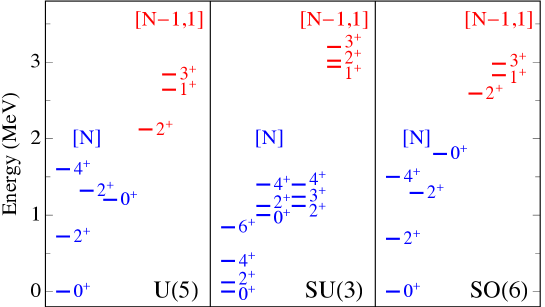
The existence of these states with mixed symmetry, excited in a variety of reactions, is by now well established [82]. The pattern of the lowest symmetric and mixed-symmetric states is shown in figure 7. Of particular relevance are $1^{+}$ states, since these are allowed in IBM-2 but not in IBM-1. The characteristic excitation of $1^{+}$ levels is of magnetic dipole type and the IBM-2 prediction for the M1 strength to the $1^{+}$ mixed-symmetry state is [77]

$$B({\rm M}1;0^{+}_{1}\rightarrow 1^{+}_{\rm MS})={3\over{4\pi}}(g_{\nu}-g_{\pi})^{2}f(N)N_{\nu}N_{\pi},$$

where $g_{\nu}$ and $g_{\pi}$ are the boson $g$ factors. The function $f(N)$ is known analytically in the three principal limits of the IBM-2, $f(N)=0$, $8/(2N-1)$ and $3/(N+1)$ in U(5), SU(3) and SO(6), respectively. This gives a simple and reasonably accurate estimate of the total M1 strength of orbital nature to $1^{+}$ mixed-symmetry states in even–even nuclei.

The geometric interpretation of mixed-symmetry states can be found by taking the limit of large boson number [83]. From this analysis emerges that they correspond to oscillations in which the neutrons and protons are out of phase, in contrast to the symmetric IBM-2 states for which such oscillations are in phase. The occurrence of such states was first predicted in the context of geometric two-fluid models in vibrational [84] and deformed [85] nuclei in which they appear as neutron–proton counter oscillations. Because of this geometric interpretation, mixed-symmetry states are often referred to as scissors states which is the pictorial image one has in the case of deformed nuclei. The IBM-2 thus confirms these geometric descriptions but at the same time generalizes them to all nuclei, not only spherical and deformed, but $\gamma$ unstable and transitional as well.

5.2 Neutrons and protons: Isospin

If neutrons and protons occupy different valence shells, it is natural to consider neutron–neutron and proton–proton pairs only, and to include the neutron–proton interaction explicitly between the two types of pairs. If neutrons and protons occupy the same valence shell, this approach no longer is valid since there is no reason not to include the $T=1$ neutron–proton pair. The ensuing model, proposed by Elliott and White [86], is called IBM-3. Because the IBM-3 includes the complete $T=1$ triplet, it can be made isospin invariant, enabling a more direct comparison with the shell model.

In the IBM-3 there are three kinds of bosons ($\nu$, $\delta$ and $\pi$) each with six components and, as a result, an $N_{\rm b}$-boson state belongs to the symmetric irreducible representation $[N_{\rm b}]$ of U(18). It is possible to construct IBM-3 states that have good total angular momentum $J$ and good total isospin $T$.

The classification of dynamical symmetries of IBM-3 is rather complex and as yet their analysis is incomplete. The cases with dynamical U(6) symmetry [or SU(3) charge symmetry] were studied in detail in reference [87]. Other classifications that conserve $J$ and $T$ [but not charge SU(3)] were proposed and analyzed in references [88, 89].

All bosons included in IBM-3 have $T=1$ and, in principle, other bosons can be introduced that correspond to $T=0$ neutron–proton pairs. This further extension (proposed by Elliott and Evans [90] and referred to as IBM-4) can be considered as the most elaborate version of the IBM. There are several reasons for including also $T=0$ bosons. One justification is found in the $LS$-coupling limit of the nuclear shell model, where the two-particle states of lowest energy have orbital angular momenta $L=0$ and $L=2$ with $(S,T)=(0,1)$ or (1,0). Furthermore, the choice of bosons in IBM-4 allows a boson classification containing Wigner’s supermultiplet algebra SU(4). These qualitative arguments in favour of IBM-4 have been corroborated by quantitative, microscopic studies in even–even [91] and odd–odd [92] $sd$-shell nuclei.

Arguably the most important virtue of the extended versions IBM-3 and IBM-4 is that they allow the construction of dynamical symmetries in the IBM with quantum numbers that have their counterparts in the shell model (isospin, Wigner supermultiplet labels, etc.). As so often emphasized by Elliott [93], this feature allows tests of the validity of the IBM in terms of the shell model.

5.3 Supersymmetry

Symmetry techniques can be applied to systems of interacting bosons and to systems of interacting fermions. In both cases the dynamical algebra is ${\rm U}(\Omega)$, with $\Omega$ the number of states available to a single particle. In both cases solvable models can be constructed from the study of the subalgebras of ${\rm U}(\Omega)$. Not surprisingly, the same symmetry techniques can be applied to systems composed of interacting bosons and fermions. If the bosons and fermions commute, the dynamical algebra of the boson–fermion system is ${\rm U}^{\rm B}(\Omega_{\rm b})\otimes{\rm U}^{\rm F}(\Omega_{\rm f})$, and the study of its subalgebras again leads to solvable hamiltonians.

This idea was applied in the context of the interacting boson–fermion model (IBFM) which proposes a description of odd-mass nuclei by coupling a fermion to a bosonic core [94]. Properties of even–even and odd-mass nuclei can be obtained from IBM and IBFM, respectively, but no unified description is achieved with the dynamical algebra ${\rm U}^{\rm B}(6)\otimes{\rm U}^{\rm F}(\Omega)$ which does not contain both types of nuclei in a single of its irreducible representations. Nuclear supersymmetry provides a theoretical framework where bosonic and fermionic systems are treated as members of the same supermultiplet and where excitation spectra of the different nuclei arise from a single hamiltonian. A necessary condition for such an approach to be successful is that the energy scale for bosonic and fermionic excitations is comparable which is indeed the case in nuclei. Nuclear supersymmetry was originally postulated by Iachello and co-workers [95, 96, 97, 98] as a symmetry among doublets and was subsequently extended to quartets of nuclei which include an odd–odd member [99].

Schematically, states in even–even and odd-mass nuclei are connected by the generators

$$\left(\begin{array}[]{c|c}b^{\dagger}b&0\\ ---&---\\ 0&a^{\dagger}a\end{array}\right),$$

where $a$ ($b$) refers to a fermion (boson) and indices are omitted for simplicity. States in an even–even nucleus are connected by the operators in the upper left-hand corner while those in odd-mass nuclei require both sets of generators. No operator connects even–even to odd-mass states. An extension of this algebraic structure considers in addition operators that transform a boson into a fermion or vice versa,

$$\left(\begin{array}[]{c|c}b^{\dagger}b&b^{\dagger}a\\ ---&---\\ a^{\dagger}b&a^{\dagger}a\end{array}\right).$$

This set does not any longer form a classical Lie algebra which is defined in terms of commutation relations. For example,

$$[a^{\dagger}b,b^{\dagger}a]=a^{\dagger}bb^{\dagger}a-b^{\dagger}aa^{\dagger}b=a^{\dagger}a-b^{\dagger}b+2b^{\dagger}ba^{\dagger}a,$$

which does not close into the original set $\{a^{\dagger}a,b^{\dagger}b,a^{\dagger}b,b^{\dagger}a\}$. The inclusion of the cross terms does not lead to a classical Lie algebra since the bilinear operators $b^{\dagger}a$ and $a^{\dagger}b$ do not behave like bosons but rather as fermions, in contrast to $a^{\dagger}a$ and $b^{\dagger}b$, both of which have bosonic character. This suggests the separation of the generators in two sectors, the bosonic sector $\{a^{\dagger}a,b^{\dagger}b\}$ and the fermionic sector $\{a^{\dagger}b,b^{\dagger}a\}$. Closure is maintained by considering anti-commutators among the latter operators and commutators otherwise. This leads to the graded or superalgebra is ${\rm U}(6/\Omega)$, where 6 and $\Omega$ are the dimensions of the boson and fermion algebras.

By embedding ${\rm U}^{\rm B}(6)\otimes{\rm U}^{\rm F}(\Omega)$ into a superalgebra ${\rm U}(6/\Omega)$, the unification of the description of even–even and odd-mass nuclei is achieved. Formally, this can be seen from the reduction

$$\begin{array}[]{ccccc}{\rm U}(6/\Omega)&\supset&{\rm U}^{\rm B}(6)&\otimes&{\rm U}^{\rm F}(\Omega)\\ \downarrow&&\downarrow&&\downarrow\\[0.0pt] [{\cal N}\}&&[N_{\rm b}]&&[1^{N_{\rm f}}]\end{array}.$$

The supersymmetric irreducible representation $[{\cal N}\}$ of ${\rm U}(6/\Omega)$ imposes symmetry in the bosons and anti-symmetry in the fermions, and contains the ${\rm U}^{\rm B}(6)\otimes{\rm U}^{\rm F}(\Omega)$ irreducible representations $[N_{\rm b}]\times[1^{N_{\rm f}}]$ with ${\cal N}=N_{\rm b}+N_{\rm f}$ [96]. A single supersymmetric irreducible representation therefore contains states in even–even ($N_{\rm f}=0$) as well as odd-mass ($N_{\rm f}=1$) nuclei.

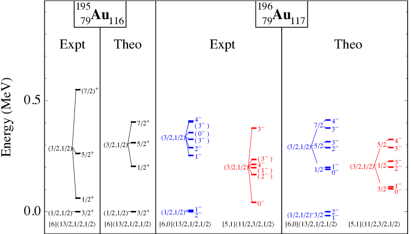
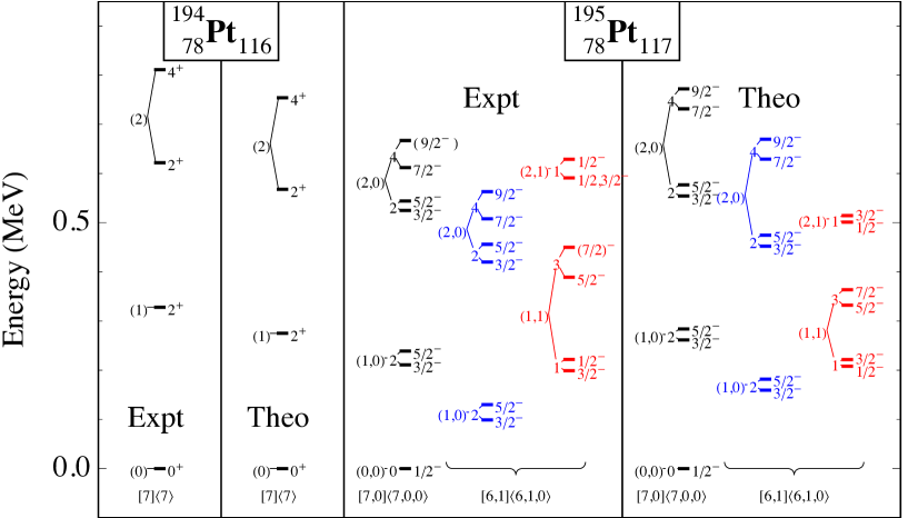
Finally, if a distinction is made between neutrons and protons, it is natural to propose a generalized dynamical algebra ${\rm U}_{\nu}(6/\Omega_{\nu})\otimes{\rm U}_{\pi}(6/\Omega_{\pi})$ where $\Omega_{\nu}$ and $\Omega_{\pi}$ are the dimensions of the neutron and proton single-particle spaces, respectively. This algebra contains generators which transform bosons into fermions and vice versa, and furthermore are distinct for neutrons and protons. The supermultiplet now contains a quartet of nuclei (even–even, even–odd, odd–even and odd–odd) which are to be described simultaneously with a single hamiltonian. The predictions of ${\rm U}_{\nu}(6/12)\otimes{\rm U}_{\pi}(6/4)$ have been extensively investigated in platinum ($Z=78$) and gold ($Z=79$) nuclei, where the dominant orbits are $3p_{1/2}$, $3p_{3/2}$ and $2f_{5/2}$ for the neutrons, and $2d_{3/2}$ for the protons. Probing the properties of the odd–odd member of the quartet proved to be a challenge and it took many years of dedicated experiments to establish a convincing case of a complete supermultiplet [100] which is shown in figure 8.

Figure 8: Example of a ${\rm U}_{\nu}(6/12)\otimes{\rm U}_{\pi}(6/4)$ supermultiplet.

6 Beyond exact solvability

The exact solutions discussed in this review are restricted to particular hamiltonians of the nuclear shell model, the geometric collective model and the interacting boson model. This concluding section contains a succinct and qualitative discussion of model hamiltonians that are not exactly solvable for all eigenstates but only for a subset of them.

It is well known that only a limited number of potentials in quantum mechanics are analytically solvable, meaning that the entire energy spectrum of eigenvalues and corresponding eigenfunctions can be obtained as exact solutions. A wider class of potentials can be constructed, with an exact solution for a finite (or possibly infinite) but not complete part of the eigenvalue spectrum. Models with such potentials are called quasi-exactly solvable (QES). This is a rich field of research that has been studied since many years (see, e.g., reference [49] and references therein). Very few QES applications were considered up to now in nuclear structure, one of which was cited in the context of the Bohr hamiltonian [47].

A related generalization concerns dynamical symmetries. The conditions for a dynamical symmetry are seldom satisfied in the description of complex quantum many-body systems. A more realistic description requires the breaking of the dynamical symmetry by adding, in a particular subalgebra chain, one or more terms from a different chain. This, in general, results in the loss of complete solvability. Nevertheless, hamiltonians with a partial dynamical symmetry (PDS) can be constructed, such that a subset of its eigenstates is characterized by a subset of the labels of a particular dynamical symmetry. The generic mechanism is layed out precisely by Alhassid and Leviatan [101] and extensively discussed in the review of Leviatan [102]. Three types of PDS exist depending on whether all (or part) of the eigenstates carry all (or part) of the quantum numbers associated with the dynamical symmetry.

Many nuclei can be described as exhibiting a transition between two dynamical symmetries (e.g., in IBM from U(5) to SU(3) or from U(5) to O(6), or a transition from pairing SU(2) to rotor SU(3), etc.). Although the transitional hamiltonian in general does not have a dynamical symmetry, it turns out that, except for a very narrow region before (or after) the transition point, the initial (or final) symmetry remains intact in some effective way. This is possible because of the existence of a quasi-dynamical symmetry (QDS) [103, 104, 105], formulated in a precise way by Rowe et al. using the concept of embedded representations [106]. Strictly speaking a hamiltonian with QDS is not exactly solvable. However, the concept of QDS clearly emanates from that of dynamical symmetry, with applications in the study of atomic nuclei [61] and of more general systems [107].

Further reading

Scientific studies covering a period of almost 80 years are difficult to summarize in barely 30 pages and consequently most developments were only fleetingly discussed in the present review. It is therefore appropriate to end with a list of suggestions for further reading. Many books exist on symmetries in physics and group theory. A standard monograph is the one of Hamermesh [108]; a more recent one in the spirit of this review is by Iachello [109]. Nuclear structure is comprehensively covered in the standard works by Bohr and Mottelson [110, 111] and the many-body techniques used in the field are discussed by Ring and Schuck [112]. Details on the shell model can be found in references [113, 114] while the interacting boson model is covered in references [114, 115, 116]. A recent monograph [117] gives an overview of symmetries encountered in the description of atomic nuclei. Finally, a discussion on embedding algebraic collective models within a shell-model framework can be found in the book of Rowe and Wood [118].

References

- [1] A. Koestler, cited by Sir Peter Medawar in The Art of the Soluble (Methuen, London, 1967).
- [2] M. Bender, P.-H. Heenen and P.G. Reinhard, Rev. Mod. Phys. 75 (2003) 121.
- [3] E. Caurier, G. Martínez–Pinedo, F. Nowacki, A. Poves and A.P. Zuker, Rev. Mod. Phys. 77 (2005) 427.
- [4] G. Racah, Phys. Rev. 63 (1943) 367.
- [5] G. Racah, Phys. Rev. 76 (1949) 1352.
- [6] A.K. Kerman, Ann. Phys. (NY) 12 (1961) 300.
- [7] K. Helmers, Nucl. Phys. 23 (1961) 594.
- [8] J. Bardeen, L.N. Cooper and J.R. Schrieffer, Phys. Rev. 106 (1957) 162 & 108 (1957) 1175.
- [9] A. Bohr, B.R. Mottelson and D. Pines, Phys. Rev. 110 (1958) 936.
- [10] R.W. Richardson, Phys. Lett. 3 (1963) 277.
- [11] J. Dukelsky, C. Esebbag and P. Schuck, Phys. Rev. Lett. 87 (2001) 066403.
- [12] F. Pan, J.P. Draayer and W.E. Ormand, Phys. Lett. B 422 (1998) 1.
- [13] A.B. Balantekin and Y. Pehlivan, Phys. Rev. C 76 (2007) 051001(R).
- [14] I. Talmi, Nucl. Phys. A 172 (1971) 1.
- [15] B.H. Flowers, Proc. Roy. Soc. (London) A 212 (1952) 248.
- [16] G. Racah, L. Farkas Memorial Volume, (Research council of Israel, Jerusalem, 1952), p. 294.
- [17] K.T. Hecht, Phys. Rev. 139 (1965) B794; Nucl. Phys. A 493 (1989) 29.
- [18] B.H. Flowers and S. Szpikowski, Proc. Phys. Soc. 84 (1964) 673.
- [19] S.C. Pang, Nucl. Phys. A 128, 497 (1969) 497.
- [20] J. Dobeš and S. Pittel, Phys. Rev. C 57 (1998) 688.
- [21] E.P. Wigner, Phys. Rev. 51 (1937) 106.
- [22] J.P. Elliott, Proc. Roy. Soc. (London) A 245 (1958) 128 & 562.
- [23] A.P. Zuker, J. Retamosa, A. Poves and E. Caurier, Phys. Rev. C 52 (1995) R1741.
- [24] K.T. Hecht and A. Adler, Nucl. Phys. A 137 (1969) 129.
- [25] A. Arima, M. Harvey and K. Shimizu, Phys. Lett. B 30 (1969) 517.
- [26] R.D. Ratna Raju, J.P. Draayer and K.T. Hecht, Nucl. Phys. A 202 (1973) 433.
- [27] J.N. Ginocchio, Phys. Rev. Lett. 78 (1997) 436.
- [28] G. Rosensteel and D.J. Rowe, Phys. Rev. Lett. 38 (1977) 10.
- [29] H.J. Lipkin, N. Meshkov and A.J. Glick, Nucl. Phys. 62 211 (1965) 188.
- [30] Lord Rayleigh, Proc. Roy. Soc. (London) 29 (1879) 71.
- [31] C.F. von Weizsäcker, Z. Phys. 96 (1935) 431.
- [32] J. Rainwater, Phys. Rev. 79 (1950) 432.
- [33] A. Bohr, K. Dansk. Vidensk. Selsk. Mat.-Fys. Meddr. 26 (1952) no 14.
- [34] A. Bohr and B.R. Mottelson, K. Dansk. Vidensk. Selsk. Mat.-Fys. Meddr. 27 (1953) no 16.
- [35] L. Wilets and M. Jean, Phys. Rev. 102 (1956) 788.
- [36] G. Rakavy, Nucl. Phys. 4 (1957) 289.
- [37] E. Chacón, M. Moshinsky and R.T. Sharp, J. Math. Phys. 17 (1976) 668.
- [38] D.J. Rowe and V. Bahri, J. Phys. A 31 (1998) 4947.
- [39] F. Iachello, Phys. Rev. Lett. 85 (2000) 3580.
- [40] P.M. Davidson, Proc. Roy. Soc. (London) 135 (1932) 459.
- [41] D. Bonatsos, P. Georgoudis, D. Lenis, N. Minkov and C. Quesne, Phys. Lett. B 683 (2010) 264.
- [42] F. Cooper, A. Khare and U. Sukhatme, Phys. Rep. 251 (1995) 267.
- [43] B. Bagchi, A. Banerjee, C. Quesne and V.M. Tkachuk, J. Phys. A 38 (2005) 2929.
- [44] L. Fortunato and A. Vitturi, J. Phys. G 29 (2003) 1341.
- [45] L. Fortunato, Eur. Phys. J. A 26 s01 (2005) 1.
- [46] D. Bonatsos, D. Lenis and D. Petrelis, Rom. Reports Phys. 59 (2007) 273.
- [47] G. Lévai and J.M. Arias, Phys. Rev. C 69 (2004) 014304.
- [48] A.V. Turbiner, Commun. Math. Phys. 118 (1988) 467.
- [49] A.G. Ushveridze, Quasi-Exactly Solvable Models in Quantum Mechanics (Institute of Physics, Bristol, 1994).
- [50] J.N. Ginocchio, Nucl. Phys. A 376 (1980) 438.
- [51] F. Reiche, Z. Phys. 39 (1926) 444.
- [52] H. Casimir, Rotation of a Rigid Body in Quantum Mechanics, PhD thesis, Rijksuniversiteit Leiden (1931).
- [53] A.S. Davydov and G.F. Filippov, Nucl. Phys. 8 (1958) 237.
- [54] A.S. Davydov and V.S. Rostovsky, Nucl. Phys. 12 (1959) 58.
- [55] S. De Baerdemacker, The Geometrical Bohr–Mottelson model: Analytic Solutions and an Algebraic Cartan–Weyl Perspective, PhD thesis, University of Ghent (2007).
- [56] A.S. Davydov and A.A. Chaban, Nucl. Phys. 20 (1960) 499.
- [57] A.S. Davydov, Nucl. Phys. 24 (1961) 682.
- [58] J. Meyer-ter-Vehn, Nucl. Phys. A 249 (1975) 111.
- [59] F. Iachello, Phys. Rev. Lett. 87 (2001) 052502.
- [60] F. Iachello, Phys. Rev. Lett. 91 (2003) 132502.
- [61] P. Cejnar, J. Jolie and R.F. Casten, Rev. Mod. Phys. 82 (2010) 014308.
- [62] S. De Baerdemacker, L. Fortunato, V. Hellemans and K. Heyde, Nucl. Phys. A769 (2006) 16.
- [63] G. Gneuss and W. Greiner, Nucl. Phys. A171 (1971) 449.
- [64] D.J. Rowe, Nucl. Phys. A735 (2004) 372.
- [65] S. De Baerdemacker, V. Hellemans and K. Heyde, J. Phys. A40 (2007) 2733.
- [66] M.A. Caprio, Phys. Rev. C 83 (2011) 064309.
- [67] A. Arima and F. Iachello, Phys. Rev. Lett. 35 (1975) 1069.
- [68] T. Otsuka, A. Arima and F. Iachello, Nucl. Phys. A 309 (1978) 1.
- [69] O. Castaños, E. Chacón, A. Frank and M. Moshinsky, J. Math. Phys. 20 (1979) 35.
- [70] A. Arima and F. Iachello, Ann. Phys. (NY) 99 (1976) 253.
- [71] A. Arima and F. Iachello, Ann. Phys. (NY) 111 (1978) 201.
- [72] A. Arima and F. Iachello, Ann. Phys. (NY) 123 (1979) 468.
- [73] J.N. Ginocchio and M.W. Kirson, Phys. Rev. Lett. 44 (1980) 1744.
- [74] A.E.L. Dieperink, O. Scholten and F. Iachello, Phys. Rev. Lett. 44 (1980) 1747.
- [75] A. Bohr and B.R. Mottelson, Phys. Scripta 22 (1980) 468.
- [76] A. Arima, T. Otsuka, F. Iachello and I. Talmi, Phys. Lett. B 66 (1977) 205.
- [77] P. Van Isacker, K. Heyde, J. Jolie and A. Sevrin, Ann. Phys. (NY) 171 (1986) 253.
- [78] J.P. Elliott and J.A. Evans, Phys. Lett. B 195 (1987) 1.
- [79] P. von Brentano, A. Gelberg, H. Harter and P. Sala, J. Phys. G: Nucl. Part. Phys. 11 (1985) L85.
- [80] F. Iachello, Phys. Rev. Lett. 53 (1984) 1427.
- [81] D. Bohle, A. Richter, W. Steffen, A.E.L. Dieperink, N. Lo Iudice, F. Palumbo and O. Scholten, Phys. Lett. B 137 (1984) 27.
- [82] K. Heyde, P. von Neumann–Cosel and A. Richter, Rev. Mod. Phys. 82 (2010) 2365.
- [83] J.N. Ginocchio and A. Leviatan, Ann. Phys. (NY) 216 (1992) 152.
- [84] A. Faessler, Nucl. Phys. A 85 (1966) 653.
- [85] N. Lo Iudice and F. Palumbo, Phys. Rev. Lett. 53 (1978) 1532.
- [86] J.P. Elliott and A.P. White, Phys. Lett. B 97 (1980) 169.
- [87] J.E. García–Ramos and P. Van Isacker, Ann. Phys. (NY) 274 (1999) 45.
- [88] J.N. Ginocchio, Phys. Rev. Lett. 77 (1996) 28.
- [89] V.K.B. Kota, Ann. Phys. (NY) 265 (1998) 101.
- [90] J.P. Elliott and J.A. Evans, Phys. Lett. B 101 (1981) 216.
- [91] P. Halse, J.P. Elliott and J.A. Evans, Nucl. Phys. A 417 (1984) 301.
- [92] P. Halse, Nucl. Phys. A 445 (1985) 93.
- [93] J.P. Elliott, Rep. Prog. Phys. 48 (1985) 171.
- [94] F. Iachello and O. Scholten, Phys. Rev. Lett. 43 (1979) 679.
- [95] F. Iachello, Phys. Rev. Lett. 44 (1980) 772.
- [96] A.B. Balantekin, I. Bars and F. Iachello, Phys. Rev. Lett. 47 (1981) 19; Nucl. Phys. A370 (1981) 284.
- [97] A.B. Balantekin, A Study of Dynamical Supersymmetries in Nuclear Physics, PhD thesis, Yale University (1982).
- [98] R. Bijker, Dynamical Boson–Fermion Symmetries in Nuclei, PhD thesis, University of Groningen (1984).
- [99] P. Van Isacker, J. Jolie, K. Heyde and A. Frank, Phys. Rev. Lett. 54 (1985) 653.
- [100] A. Metz, J. Jolie, G. Graw , R. Hertenberger, J. Gröger, C. Günther, N. Warr and Y. Eisermann, Phys. Rev. Lett. 83 (1999) 1542.
- [101] Y. Alhassid and A. Leviatan, J. Phys. A 25 (1992) L1265.
- [102] A. Leviatan, Prog. Part. Nucl. Phys. 66 (2011) 93.
- [103] D.J. Rowe, Nucl. Phys. A 745 (2004) 47.
- [104] P.S. Turner and D.J. Rowe, Nucl. Phys. A 756 (2005) 333.
- [105] G. Rosensteel and D.J. Rowe, Nucl. Phys. A 759 (2005) 92.
- [106] D.J. Rowe, P. Rochford and J. Repka, J. Math. Phys. 29 (1988) 572.
- [107] D. Rowe, M.J. Carvalho and J. Repka, Rev. Mod. Phys. 84 (2012) 711.
- [108] M. Hamermesh, Group Theory and Its Application to Physical Problems (Addison–Wesley, Reading MA, 1962).
- [109] F. Iachello, Lie Algebras and Applications. Lecture Notes in Physics (Springer–Verlag, Berlin, 2006).
- [110] A. Bohr and B.R. Mottelson, Nuclear Structure. I Single-Particle Motion (Benjamin, New York, 1969).
- [111] A. Bohr and B.R. Mottelson, Nuclear Structure. II Nuclear Deformations (Benjamin, New York, 1975).
- [112] P. Ring and P. Schuck, The Nuclear Many-Body Problem (Springer Verlag, New York, 1980).
- [113] K.L.G. Heyde, The Nuclear Shell Model (Springer-Verlag, Berlin, 1990).
- [114] I. Talmi, Simple Models of Complex Nuclei. The Shell Model and Interacting Boson Model (Harwood, Chur, 1993).
- [115] F. Iachello and A. Arima, The Interacting Boson Model (Cambridge University Press, Cambridge, 1987).
- [116] F. Iachello and P. Van Isacker, The Interacting Boson–Fermion Model (Cambridge University Press, Cambridge, 1991).
- [117] A. Frank, J. Jolie and P. Van Isacker, Symmetries in Atomic Nuclei. From Isospin to Supersymmetry (Springer Science, New York, 2009).
- [118] D.J. Rowe and J.L. Wood, Fundamentals of Nuclear Models. Foundational Models (World Scientific, Singapore, 2010).