Comparing the Performance of Different x86 SIMD Instruction Sets for a Medical Imaging Application on Modern Multi- and Manycore Chips

Abstract

Single Instruction, Multiple Data (SIMD) vectorization is a major driver of performance in current architectures, and is mandatory for achieving good performance with codes that are limited by instruction throughput. We investigate the efficiency of different SIMD-vectorized implementations of the RabbitCT benchmark. RabbitCT performs 3D image reconstruction by back projection, a vital operation in computed tomography applications. The underlying algorithm is a challenge for vectorization because it consists, apart from a streaming part, also of a bilinear interpolation requiring scattered access to image data. We analyze the performance of SSE (128 bit), AVX (256 bit), AVX2 (256 bit), and IMCI (512 bit) implementations on recent Intel x86 systems. A special emphasis is put on the vector gather implementation on Intel Haswell and Knights Corner microarchitectures. Finally we discuss why GPU implementations perform much better for this specific algorithm.

1 Introduction

Single Instruction, Multiple Data (SIMD) is a data-parallel execution model enabling to do more work with the same number of instructions. Because of its integration in existing microarchitectures it is a standard technology for increasing performance in modern processors. While the idea originated in the early seventies, the first implementation in a commodity processor was Intel’s MMX instruction set extension for the x86 Pentium processor line in 1996. With AltiVec/VMX (1998) for PowerPC and SSE (1999) for x86 more capable 128 bit-wide SIMD instruction set extensions followed. For the software the introduction of SIMD was a paradigm shift as in contrast to previous hardware optimizations, which were designed to work transparently, the software must make explicit use of the new instructions in order to leverage the full potential of new processors. Vendors promised that optimizing compilers would enable the efficient use of the new instructions, but it soon turned out that in many cases data structures must be adapted and kernels must be rewritten with the help of compiler intrinsics or even in assembly code. Intel incrementally updated the SIMD capabilities by introducing new instruction set extensions. SSE comprised 70 instructions, SSE2 (2001) added 144, SSE3 (2004) 29, and SSE4 (2006) 54 new instructions, for a total of 297 instructions Intel Corporation [2013]. In 2011 Intel doubled the SIMD width to 256 bit with AVX. Still of the total 349 instructions introduced with AVX only a subset of 92 instructions supported the 256 bit registers and only few new instructions were added. This was changed in 2013 with AVX2, which promoted most instructions to 256 bit and again added new ones. The new instructions can be grouped into complex instructions for arithmetic targeted at specific application classes, horizontal operations, more powerful in-register reordering instructions, and operations promoted to vectorized execution. While most of this can be seen as incremental improvements, AVX2 introduces instructions that change the way SIMD can be employed. This is the gather instruction together with the ability to mask out SIMD lanes with predicate registers. The hope is that this enables the use of SIMD in new application classes with more complex data access patterns where SIMD could not be used efficiently up to now. The first implementation of the AVX2 instruction set is in the Intel Haswell microarchitecture. Haswell also features Fused Multiply-Add (FMA) instructions in a separate instruction set extension (FMA3).

In 2006 Intel started developing an x86 many-core design (codename Larrabee), initially targeted as an alternative to existing graphics processors. It uses a 512 bit SIMD instruction set called IMCI (Initial Many Core Instructions). While in 2010 the usage as a GPU was terminated, the design was refined and eventually re-targeted as an accelerator card. The first product based on this design, the Intel Xeon Phi, was available in early 2013 with 60 cores and 8 GB of main memory. IMCI already anticipated and implemented many current developments in SIMD instruction sets and allowed to gain experience with a working implementation. The instruction set comprises gather/scatter instructions, predicate registers, and FMA.

This paper studies the efficiency of an important algorithm from medical imaging when mapped to different Intel SIMD instruction set extensions. We look at the Instruction Set Architecture (ISA) interface as well as its implementation in a concrete microarchitecture. Although we also present results for compiler-generated code, a detailed analysis of the conditions under which a compiler would be able to achieve the same performance level as hand-crafted assembly is out of scope for this paper. Still we discuss how well an instruction set extension is suited for automatic generation of efficient code.

We have chosen the RabbitCT benchmarking framework as test case Rohkohl et al. [2009]. RabbitCT implements volume reconstruction by back projection, which is the performance limiting part of many Computed Tomography (CT) applications. This operation is well suited for evaluating SIMD implementations, because it consists of streaming as well as scattered data access patterns and is therefore non-trivial to vectorize. Although a naive performance model suggests that the runtime of the algorithm should be determined by main memory bandwidth, its implementation with existing instruction sets introduces so much overhead that instruction throughput becomes the bottleneck. Therefore it can be seen as a prototype for applications in which the data cannot be loaded block-wise, but instead requires in-register shuffles. An interesting aspect of RabbitCT is that it is also a popular target for GPU-based efforts and therefore provides a good case to compare general purpose multi- and manycore designs with GPUs.

We picked an Intel Xeon IvyBridge-EP two-socket system for executing the SSE and AVX code variants and an Intel Xeon Phi accelerator card for the IMCI kernels. Unfortunately a multi-socket system implementing AVX2 and FMA3 is not yet available. Therefore we choose a single socket Intel Xeon Haswell system to execute the AVX2/FMA3 kernel.

This paper is structured as follows. Section 2 gives an overview of previous work about the performance optimization of this algorithm. The test systems used are described in Section 3. Section 4 introduces the RabbitCT benchmark and motivates its use for this study. Next we cover the SIMD kernel implementations in Section 5. We briefly introduce all optimizations applied and specifically cover the SIMD vectorization with an emphasis on the gather instruction in IMCI and AVX2. The section closes with a detailed instruction code analysis for the resulting kernels. The results are presented in Section 6. We separate single core from full system results to be able to clearly analyze the SIMD speedup efficiency. We also present microbenchmarking results showing the instruction latency for different settings in the current gather implementations. In Section 7 we compare our results with the fastest published GPU result and try to explain why this specific application is well suited for GPUs. We also present performance numbers for generated code in Section 8. To conclude we summarize our results and give an outlook.

2 Related Work

Due to its relevance in medical applications, reconstruction in computed tomography is a well-studied problem. As vendors for CT devices are constantly looking for ways to speed up the reconstruction time, many computer architectures have been evaluated over time. Initial products in this field used special purpose hardware based on FPGAs (Field Programmable Gate Arrays) and DSPs (Digital Signal Processors) Heigl and Kowarschik [2007]. The Cell Broadband Engine, which at the time of its release provided unrivaled memory bandwidth, was also subject to experimentation Kachelriess et al. [2007]; Scherl et al. [2012]. It is noteworthy that CT reconstruction was among the first non-graphics applications that were run on graphics processors Pratx and Xing [2011]. However, the use of varying data sets and reconstruction parameters limited the comparability of all these implementations. In an attempt to remedy this problem, the RabbitCT framework Rohkohl et al. [2009] provides a standardized, freely available CT scan data set and a uniform benchmarking interface that evaluates both reconstruction performance and accuracy. Current noteworthy entries in the RabbitCT ranking include Thumper by Zinsser and Keck Zinsser and Keck [2013], a Kepler-based implementation which currently dominates all other implementations, and fastrabbit by Treibig et al. Treibig et al. [2013], a highly optimized CPU-based implementation. The presented work is partly based on the results of fastrabbit, improving it and providing an implementation for the Intel IMCI and AVX2 instruction sets.

3 Experimental Testbed

Microarchitecture	Intel IvyBridge-EP	Intel Haswell	Intel Knights Corner
Model	Xeon E5-2660 v2	Xeon E3-1240 v3	Xeon Phi 5110P
Base/Max. Turbo Clock Speed	2.2 GHz/3.0 GHz	3.4 GHz/3.8 GHz	1.053 GHz/–
Sockets/Cores/Threads per Node	2/20/40	1/4/8	1/60/240
SIMD Support	SSE (128 bit), AVX (256 bit)	AVX2 (256 bit), FMA3 (256 bit)	IMCI (512 bit)
Vector Register File	16 Registers	16 Registers	32 Registers
Node L1/L2/L3 Cache	20$\times$32 kB/20$\times$256 kB/2$\times$25 MB	4$\times$32 kB/4$\times$256 kB/8 MB	60$\times$32 kB/60$\times$512 kB/–
Node Main Memory Configuration	8 channels DDR3-1866	2 channels DDR3-1600	16 channels GDDR5 5GHz
Node Peak Memory Bandwidth	119.4 GB/s	25.6 GB/s	320 GB/s
Node Update Benchmark Bandwidth	98 GB/s (81%)	23 GB/s (90%)	168 GB/s (53%)

Table 1: Test machine specifications. “Node Update” is a streaming multi-threaded benchmark that modifies an array in memory.

A standard two-socket server based on the IvyBridge-EP microarchitecture was chosen for executing the SSE/AVX kernels. It employs two-way SMT and has ten moderately clocked (2.2 GHz base frequency) cores per socket. Sixteen vector registers are available for use with SSE and AVX. Using floating-point arithmetic, each core can execute one multiply and one add instruction per cycle, leading to a peak performance of eight Double Precision (DP) or 16 Single Precision (SP) Flops per cycle. Memory bandwidth is provided by means of a ccNUMA memory subsystem with four DDR3-1600 memory channels per socket.

For the AVX2/FMA3 kernel a single-socket Intel Xeon server based on the Haswell microarchitecture was used. This system has four cores (two-way SMT) and 8 MB of L3 cache.

The Intel Xeon Phi is located on a PCIe card and runs its own operating system. It consists of a single chip providing 60 low-frequency cores with four-way SMT. The cores are based on a modified version of P54C design used in the original Pentium processor (1995). Each core is in-order and two-way superscalar, featuring a scalar pipeline (V-pipe) and a vector pipeline (U-pipe). The Vector Processing Unit (VPU) connected to the U-pipe features a total of 32 512 bit vector registers and is capable of FMA operations, yielding a total of 16 DP (32 SP) Flops per cycle. The cores are connected via a bidirectional ring bus. Eight GDDR5 memory controllers with two channels each are connected to the ring bus. The Xeon Phi offers different settings for usage, such as offload (common for GPUs) and native mode. We have used the native execution model in which everything is executed on the accelerator card and data transfers to and from the card are not taken into account. An overview of the test machine specifications is given in Table 1.

4 RabbitCT Benchmark

In CT an X-ray source and a flat-panel detector positioned on opposing ends of a gantry move along a defined trajectory—mostly a circle—around the volume that holds the object to be investigated. X-ray images are taken at regular angular increments along the way. In general 3D image reconstruction works by back projecting the information recorded in the individual X-ray images (also called projection images) into a 3D volume, which is made up of individual voxels (volume elements). In medical applications, this volume almost always has an extent of $512^{3}$ voxels. To obtain the intensity value for a particular voxel of the volume from one of the recorded projection images we forward project a ray originating from the X-ray source through the center of the voxel to the detector; the intensity value at the resulting detector coordinates is then read from the recorded projection image and added to the voxel. This process is performed for each voxel of the volume and all recorded projection images, yielding the reconstructed 3D volume as the result.

Performance comparisons of different optimized back projection implementations found in the literature can be difficult because of variations in data acquisition and preprocessing, as well as different geometry conversions and the use of proprietary data sets. The RabbitCT framework was designed as an open platform that tries to remedy these problems. It features a benchmarking interface, a prototype back projection implementation, and a filtered, high resolution CT dataset of a rabbit; it also includes a reference volume that is used to derive various image quality metrics. The preprocessed dataset consists of 496 projection images that were acquired using a commercial C-arm CT system. Each projection is 1248$\times$960 pixels wide and contains the filtered and weighted intensity values as single-precision floating-point numbers. In addition, each projection image $p_{i}$ comes with a separate projection matrix $A_{i}\in\mathbb{R}^{3\times 4}$, which is used to perform the forward projection. The framework takes care of all required steps to set up the benchmark, so the programmer can focus entirely on the actual back projection implementation, which is provided as a module (shared library) to the framework.

4.1 Algorithm

⬇

1for (z=0; z<L; ++z) { // iterate over all voxels

2 for (y=0; y<L; ++y) {

3 for (x=0; x<L; ++x) {

4 // PART 1

5 // convert from VCS to WCS

6 float wx = O + x * MM;

7 float wy = O + y * MM;

8 float wz = O + z * MM;

9 // convert from WCS to ICS

10 float u = wx*A[0] + wy*A[3] + wz*A[6] + A[9];

11 float v = wx*A[1] + wy*A[4] + wz*A[7] + A[10];

12 float w = wx*A[2] + wy*A[5] + wz*A[8] + A[11];

13 // de-homogenize

14 float ix = u / w;

15 float iy = v / w;

16 // integer indices to access projection image

17 int iix = (int)ix;

18 int iiy = (int)iy;

19 // calculate interpolation weights

20 float scalex = ix - iix;

21 float scaley = iy - iiy;

22 // PART 2

23 // load four values for bilinear interpolation

24 float valbl = 0.0f; float valbr = 0.0f;

25 float valtr = 0.0f; float valtl = 0.0f;

26 if (iiy>=0 && iiy<width && iix>=0 && iix<height)

27 valbl = I[iiy * width + iix];

28 if (iiy>=0 && iiy<width && iix+1>=0

29 && iix+1<height)

30 valbr = I[iiy * width + iix + 1];

31 if (iiy+1>=0 && iiy+1<width && iix>=0

32 && iix<height)

33 valtl = I[(iiy + 1) * width + iix];

34 if (iiy+1>=0 && iiy+1<width && iix+1>=0

35 && iix+1<height)

36 valtr = I[(iiy + 1)* width + iix + 1];

37 // PART 3

38 // perform bilinear interpolation

39 float valb = (1-scalex)*valbl + scalex*valbr;

40 float valt = (1-scalex)*valtl + scalex*valtr;

41 float val = (1-scaley)*valb + scaley*valt;

42 // add weighted results to voxel

43 VOL[z*L*L+y*L+x] += val / (w * w);

44 } // x-loop

45 } // y-loop

46} // z-loop

Listing 1: Unoptimized reference back projection implementation processing a single projection image.

A slightly compressed version of the unoptimized reference implementation that comes with RabbitCT is shown in Listing 1. This code is called once for every projection image. The three outer for loops (lines 1–3) are used to iterate over all voxels in the volume; note that we refer to the innermost x-loop, which updates one “line” of voxels in the volume, as the “line update kernel.” The loop variables x, y, and z are used to logically address all voxels in memory. To perform the forward projection these logical coordinates used for addressing must first be converted to the World Coordinate System (WCS), whose origin coincides with the center of the voxel volume; this conversion happens in lines 6–8. The variables O and MM that are required to perform this conversion are precalculated by the RabbitCT framework and made available to the back projection implementation in a struct pointer that is passed to the back projection function as a parameter.

After this the forward projection is performed using the corresponding projection matrix in lines 10–12. In order to transform the affine mapping that implements the forward projection into a linear mapping homogeneous coordinates are used. Thus the detector coordinates are obtained in lines 14 and 15 by dehomogenization.

The next step is a bilinear interpolation, which requires converting the previously obtained detector coordinates from floating-point to integer (lines 17–18) to address the intensity values in the projection image buffer I. The interpolation weights scalex and scaley are calculated in lines 20–21.

The four intensity values needed for the bilinear interpolation are fetched from the buffer containing the intensity values in lines 26–36. The if statements ensure that the image coordinates lie inside the projection image; in case the ray does not hit the detector, i.e., if the coordinates lie outside the projection image, an intensity value of zero is assumed (lines 24–25). Note that the projection image is linearized, which is why we need the projection image width in the variable width (also made available by the framework via the struct pointer passed to the function) to correctly address data inside the buffer.

The actual bilinear interpolation is performed in lines 39–41. Before the result is written back into the volume, it is weighted according to the inverse-square law (line 43). The variable w holds the homogeneous coordinate, which is an approximation of the distance from the X-ray source to the voxel under consideration, and can be used to perform the weighting.

For all further analysis we will structure the overall algorithm in three main parts. Part 1 consists of the geometry computation involving the calculation of the index in detector coordinates. Part 2 involves of the actual loading of the intensity values from the projection image. Finally in Part 3 the bilinear interpolation and the update of the voxel data is performed.

4.2 Code Analysis

One voxel sweep incurs a data transfer volume which consists of the loads from the projection image and an update operation (VOL[i]+=s for all i) to the voxel array. The latter causes 8 bytes of traffic per voxel and for the medically relevant problem size of $512^{3}$ voxels results in a data volume of $1$ GB per projection image, or $496$ GB for all projections. The main memory traffic caused by loading the intensity values from the projection images is hard to quantify since it is not a simple stream; it is defined by a “beam” of locations slowly moving over the projection image as the voxel update loop nest progresses. It exhibits some temporal locality, which allows for a certain degree of caching, since neighboring voxels are projected on proximate regions in the image, but there may also be multiple streams with large strides if the beam sweeps across the image orthogonal to the rows. On the computational side, the basic version of this algorithm performs 13 additions, 5 subtractions, 17 multiplications, and 3 divides.

5 Implementation

Task parallel programming is based on OpenMP: The voxel volume is segmented into voxels planes that can be processed independent from each other. All line update kernels (SSE, AVX, AVX2/FMA3, IMCI) are written in assembly language and use all of the optimizations found in the original fastrabbit implementation Treibig et al. [2013].

The presented work improves on these achievements. The original algorithm calculating the clipping mask had minor flaws, which have been remedied. For a $512^{3}$ volume we can reduce the number of voxels that have to be processed by almost 10% when using the improved instead of the original clipping mask. Moreover parameter handling and instruction scheduling inside the kernel was improved leading to an overall speedup of a factor of 1.25 compared to the original fastrabbit implementation.

5.1 SIMD Vectorization

Part 1 of the algorithm is straightforward to vectorize. A viable optimization on all architectures is to replace the divide with a reciprocal instruction. The reciprocal is pipelined with a throughput of one cycle and has a lower latency compared to the standard divide. On KNC the reciprocal provides full accuracy; on the CPU, however, it has a reduced accuracy (11 bits of mantissa). Nevertheless, the quality of the resulting reconstruction is similar to that of GPU implementations. As a result of Part 1, the detector indices have been computed and are located in SIMD registers.

Part 2 is the most difficult part of the algorithm, because the required detector values are not contiguous in memory. Moreover, the contents of a SIMD register cannot be used for addressing (i.e., as pointers or offsets) in SSE and AVX. Therefore the SIMD register containing the indices must be stored back to memory and loaded again into a general purpose register for addressing. Since two adjacent values are always needed (cf. bilinear interpolation), the image data can be loaded in pairs. The interpolation weights need to be rearranged to match the order of the intensity values. While Part 2 looks simple in C code, it requires a lot of instructions to implement it efficiently using SSE and AVX. This part therefore does not scale very well with increased register width.

In Part 3 the actual bilinear interpolation is performed. It requires some additional reordering of the data in the SIMD registers, but is otherwise straightforward to vectorize. The SSE and AVX implementations are very similar, the latter requiring more reordering and adding more overhead for loading the data due to its doubled SIMD width.

The main difference between SSE/AVX and AVX2/IMCI is the availability of FMA and gather instructions in the latter. A significant part of the arithmetic operations can be mapped to FMAs. The gather instruction simplifies the implementation considerably, since it enables using the indices in the SIMD register directly for addressing. However, some peculiarities of the IMCI ISA diminish this benefit. The AVX2 implementation is very similar to IMCI but provides a much simpler interface to the gather instruction, saving 50% instructions compared to the IMCI version. Instruction set-wise, the gather instruction is a main benefit for this algorithm, so we introduce it in more detail in the following section.

5.1.1 Gather Instruction Interfaces

⬇

1 kxnor k2, k2

2..L100: vgatherdps zmm13{k2}, [rdi + zmm17 * 4]

3 jkzd k2, ..L101

4 vgatherdps zmm13{k2}, [rdi + zmm17 * 4]

5 jknzd k2, ..L100

6..L101:

Listing 2: Gather instruction interface in IMCI.

Listing 2 shows the instruction code for one gather construct with IMCI. The vgatherdps instruction loads 16 single-precision values (or fewer, depending on which bits of the mask register—k2 in our example—are set) into a register from the 16 addresses specified in its second argument. Instead of fetching all data with one instruction, vgatherdps works by getting the data cache line-wise per invocation; this means that every time the gather instruction is used, it will fetch only one cache line (CL), load all the values that it is supposed to gather from it, store them in the destination vector register, and finally zero out the bits of the components that have been filled in the vector mask register. As a consequence, the number of gather instruction depends on the distribution of the data: If all data resides in one CL then one gather instruction is sufficient; in the worst case, each value is located in a different CL, which will require sixteen gather instructions. The jkzd instruction in line 3 checks the contents of the vector mask register that was updated in the line before by the vgatherdps instruction. If the mask register is zero, i.e., all zero bits indicating that all data has been gathered, control flow continues at label ..L101 in line 6; if the mask register is non-zero, i.e., if one or more bits are set, indicating that there is still data to be fetched, no jump is performed and the vgatherdps in line 4 is scheduled next. After more data has been gathered and k2 has been updated, the vector mask register is tested again for zero by the jknzd in line 5. If there is still data to be fetched, control flow will jump back to label ..L100 in line 2, starting the gather construct all over. If all data has been fetched, the construct is left. This two-stage strategy was obtained by examining the compiler output for non-contiguous data access and turns out to be faster than a simple loop with only one gather instruction. The authors have as yet no plausible explanation for this.

⬇

1 vpcmpeqw ymm7, ymm7, ymm7

2 vgatherdps ymm15, [rdi + ymm11 * 4], ymm7

Listing 3: Gather instruction interface in AVX2.

Listing 3 shows the respective code for AVX2. In contrast to IMCI, no loop construct is required and a single instruction is sufficient. This allows for a very compact and elegant code. Instead of using dedicated vector mask registers, AVX2 uses regular vector registers (supplied as third argument) as mask for the operation.

Note that for our application we always gather all vector components without checking whether the intensity values are located inside the projection images or not. This is achieved by setting the vector (mask) registers to all one bits (kxnor, vpcmpeqw). We found that copying the projection images into a zero-padded buffer and removing the conditionals (cf. lines 26–36 in Listing 1) resulted in a better performance than setting the mask registers, which causes too much instruction overhead.

5.2 Instruction Code Analysis

The main benefit of SIMD is that a given amount of work can be finished with fewer instructions than with scalar execution. Therefore the number of instructions and their composition in terms of instruction types (memory, in-register, arithmetic, etc.) are interesting metrics for our case. These are influenced by the register width and by the availability of instruction types, such as FMA or gather instructions. Table 2 shows an overview for the three parts of this algorithm for all five hand-written assembly implementations. Note that for Haswell in addition to an AVX2 version we also devised an AVX/FMA3 implementation that uses Haswell’s FMA3 instruction but is otherwise identical to the AVX implementation—i.e. it uses no gather instructions.

Part 1 is trivial to vectorize and exhibits good scalability: In Table 2 this is reflected by the fact that hardly any additional instructions are required when switching from SSE to AVX. Apart from reducing the total number of arithmetic instructions, the use of FMA has the additional benefit of reducing memory instruction in Part 1: Because a FMA doesn’t require an intermediate register for the result of the multiplication, register pressure and—as a consequence—the amount of register spilling is lower. In contrast to the first part, the second part of the algorithm scales poorly instruction-wise. Due to the sequential loads, the number of memory operations almost doubles when switching from SSE to AVX. For IMCI the gather instruction simplifies the implementation, because no additional in-register reordering is necessary. In contrast to the slim AVX2 gather interface, the bold IMCI loop interface cancels out the advantage instruction-wise and ends up with an instruction count similar to AVX. In Part 3, while in theory simple to vectorize, all non-gather implementations suffer from in-register reordering overhead.

Overall, the overhead of switching from SSE to AVX is 19 instructions. IMCI roughly ends up with the same instruction count as the SSE code. While we would anticipate a lower instruction count for IMCI considering FMA and gather, the fact prefetching has to be implemented in software and the design of the gather interface cause a lot of instruction overhead. The AVX2 gather interface does not suffer from this shortcoming and has the lowest instruction count.

	Type	SSE	AVX	AVX2	AVX/FMA3	IMCI
Part 1	Memory	4	3	0	3	0
	Arith.	17	17	12	12	15
	All	21	20	12	15	15
Part 2	Memory	18	34	4	34	16
	Shuffle	6	10	0	10	0
	Arith.	2	2	12	2	24
	All	26	46	16	46	40
Part 3	Memory	2	2	2	2	2
	Arith.	20	20	15	16	12
	All	22	22	17	18	14
Other	All	4	4	4	3	8
Total		73	92	49	82	77

Table 2: Instruction count and composition. The instruction types are categorized into three classes: memory for all instructions with a memory reference, shuffle for register manipulation instructions, and arithmetic for computational instructions. All remaining instructions such as, e.g., loop instructions are contained in other.

In Table 3 we compare the number of instructions required by different SIMD instruction sets compared to baseline scalar code. The baseline code was generated using the Intel 13.1 compiler together with the -O3 -no-vec -x flag for each of the instruction sets. This means that for AVX and AVX2 the scalar version makes use of the new VEX (vector extensions) prefix introduced by AVX, allowing instructions to use more than two operands; the AVX2 and AVX/FMA3 versions use FMA instructions. We omit IMCI in this comparison, because there exist no dedicated scalar instructions in this instruction set. The “instruction count efficiency” metric is the ratio of instruction counts between the scalar and the vectorized code versions—e.g. an efficiency of 100% means that both versions require the same amount of instructions, whereas an efficiency of 50% means that the vectorized code requires twice as many instructions as the scalar code. Additionally we also list the “SIMD runtime efficiency,” which we define as the achieved runtime speedup divided by the number of SIMD lanes. Interestingly, the SIMD efficiency numbers for SSE and AVX are almost identical to the respective instruction count efficiencies. For both the AVX2 and AVX/FMA3 implementations the baseline scalar code was generated using the -xCORE-AVX2, which is why the AVX/FMA3 code shows a lower runtime efficiency than AVX. Interestingly we find that while instruction count efficiency is higher using AVX2, AVX/FMA3 provides better runtime efficiency, i.e. performance. The reason for this is the high latency of the gather instruction that is used in the AVX2 variant (cf. Section 6.3).

	SSE	AVX	AVX2	AVX/FMA3
Voxels per Vectorized Loop	4	8	8	8
Instr. per Loop (SIMD)	73	92	49	82
Instr. per Voxel (Scalar)	57	46	41	46
Instr. Count Efficiency	78%	50%	84%	56%
SIMD Runtime Efficiency	82%	51%	33%	42%

Table 3: Overview of static instruction code analysis. Runtime Efficiency results pertain to one core using SMT.

6 Results

Section 5.2 has already described the SIMD efficiency of various implementations in terms of instruction overhead. Here we present results illustrating how well the instruction set was implemented in the microarchitectures and how efficient the implementation is in terms of speedup. To do so we distinguish two cases: Single core (to pinpoint the SIMD influence alone) and full-system scaling. It was shown previously Treibig et al. [2013] that the performance of the code is limited by instruction execution, and that data transfers through the cache hierarchy do not play a significant role on modern multi-core architectures. Thread pinning was done with likwid-pin Treibig et al. [2010].

6.1 Analysis of SIMD and SMT Speedup

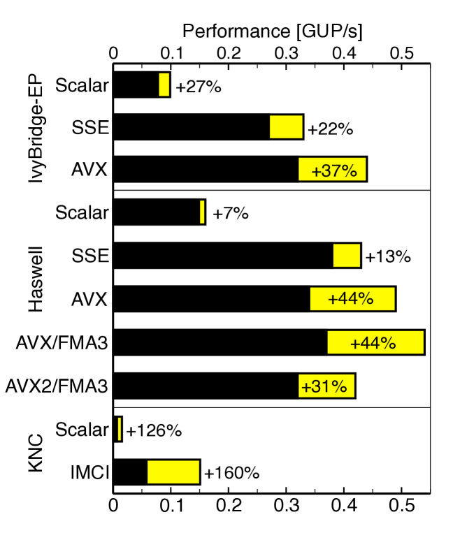
Figure 1: Single core performance of different SIMD implementations on IvyBridge-EP, Haswell and Knights Corner (KNC) in billions of voxel updates per second (GUP/s). The black bars are sequential results. The yellow bar is the speedup using all available SMT threads. The scalar version on IvyBridge-EP based on AVX and on Haswell on AVX2.

Figure 1 shows the results for single core performance. Again, scalar code was generated using the Intel 13.1 compiler. It is instructive to analyze the benefit of Simultaneous Multi-Threading (SMT) together with SIMD, since a considerable speedup with SMT points to inefficient pipeline utilization. On IvyBridge-EP, SSE yields a 3.3$\times$ speedup with SMT (out of a possible 4$\times$). As expected, the AVX kernel is significantly less efficient, with 4.1$\times$ out of 8$\times$. It is known that the AVX kernel suffers from critical path dependencies Treibig et al. [2013], which is confirmed by the large benefit gained with SMT. In a sense, inefficient SIMD code can be partly compensated by multi-threading in this particular case. On Haswell the SSE kernel performs surprisingly well, even without SMT, but the best possible variant is AVX/FMA3 with SMT. The AVX2 kernel is the slowest of all variants despite its instruction count advantage: The bilinear interpolation requires four intensity values for each voxel, which results in four gather instructions. These incur a latency of about 42 clock cycles (cf. Sec. 6.3). In contrast the AVX and AVX/FMA3 implementations use 16 pairwise loads to gather the intensity values; although these version require about 10 additional in-register shuffling instructions overall this approach yields a much better performance. On KNC the SIMD speedup is 10$\times$ out of a possible 16$\times$. This result emerges from a combination of slow scalar code (see above) with an inefficient and dominating gather instruction in the SIMD case. We will analyze the latter in more depth in Section 6.3.

6.2 Full Device Results

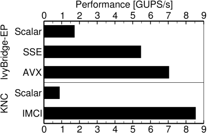
Figure 2: Full system performance on IvyBridge-EP and KNC

Figure 2 shows the performance of scalar and vectorized implementations on IvyBridge-EP and KNC. Results for Haswell are omitted because at the time of writing no two-socket system was available. The full system results were measured with Turbo mode enabled and all available SMT threads. A naive peak performance comparison gives reason to expect a 3$\times$ advantage for KNC. For our algorithm, one KNC device is only 1.2$\times$ faster than one IvyBridge-EP node. This is a disappointing result, considering that IvyBridge-EP is also available with 12 instead of 10 cores and with a faster clock speed. Both architectures suffer from the impact of the inefficient Part 2 execution, but this problem is more severe on KNC, as will be demonstrated in Section 6.4.

Scalability across the cores is very similar on both systems, with a parallel efficiency of 93%. This corroborates the expectation that code execution is highly core-bound.

6.3 Detailed Performance Analysis of Vector Gather Implementations

The vector gather instruction in the KNC microarchitecture has attracted major attention as it is the first gather implementation in an x86-based design. In this section we conduct a more detailed analysis of the gather performance on KNC, and compare with the situation on Haswell (with AVX2).

As introduced in Section 5.1.1 the KNC ISA requires the gather instructions to be invoked multiple times in order to load all required data elements. The exact number of executions depends on the total number of cache lines the data is loaded from. Using the likwid-bench tool Treibig et al. [2010] we implemented a microbenchmark which allows to measure the average instruction latency depending on how many values are loaded per call (cache line). All hardware threads of a single core were used to measure the latencies to gather 16 elements from L1 cache and L2 cache, depending on how the data is distributed. The results are shown in Table 4.

Microarchitecture	Knights Corner				Haswell
Distribution	L1 Cache		L2 Cache		L1 Cache	L2 Cache
	Instruction	Loop	Instruction	Loop	Instruction	Instruction
16 per CL	9.0	9.0	13.6	13.6
8 per CL	4.2	8.4	9.4	18.8	10.0	10.0
4 per CL	3.7	14.8	9.1	36.4	11.0	11.2
2 per CL	2.9	23.2	8.6	68.8	10.0	12.0
1 per CL	2.3	36.8	8.1	129.6	11.2	11.2

Table 4: Latencies in clock cycles encountered when gathering data from different levels of the memory hierarchy for different distributions of the data to be gathered. “Instruction” and “Loop” refer to the average latency of a single vgatherdps instruction and the total time required to gather all 16 (IMCI) or 8 (AVX2) elements, respectively.

We find that the latency for a single vgatherdps instruction on KNC varies depending on how many elements it has to fetch from a cache line. The reason for this effect is that the vgatherdps instruction itself is implemented as another loop, not visible on the ISA level: the more elements it has to fetch from a single CL, the higher the latency. Nevertheless we find that it is beneficial for the data to reside in as few CLs as possible: Although the latency for a single vgatherdps instruction increases with the number of elements per cache line, the impact of calling the vgatherdps instruction multiple times is generally more severe. On the Haswell microarchitecture, the gather latency is largely independent of the number of cache lines touched when data is in the L1 or the L2 cache. From the numbers it is evident that it may be faster in some cases to ignore the hardware-based gather. The good performance of the AVX/FMA3 algorithm implementation on Haswell compared to AVX2 (see Fig. 1) is a direct consequence of this.

On KNC, which has no L1 hardware prefetcher, there is a noticeable impact when dropping from L1 to L2 cache. Due to the streaming access pattern in the microbenchmark we find that on Haswell there is almost no difference in latency depending on whether data is gathered from L1 or L2 cache due to hardware prefetching. Overall, the performance impact of the gather operation is much more severe on KNC than on Haswell. In Section 6.4 we will show that the gather instructions do indeed account for the dominant part of the kernel runtime on KNC, leading to the observed mediocre KNC performance.

6.4 Performance Analysis for Knights Corner

We start by estimating how many cycles are needed to execute one loop iteration of the kernel. Neglecting the variable influence of the gather constructs in Part 2 for the time being, we created a variant of the full kernel without gather instructions.

Based on a static instruction code analysis taking into account instruction pairing (superscalar execution) we estimate 34 cycles for the gather-less kernel. This was verified by measurement which resulted in about 37.5 cycles. For our model, we use the measured value of 37.5 clock cycles because it contains non-negligible overhead such as backing up caller-save registers when calling the line update kernel that was not accounted for in the analytical prediction.

By instrumentation of the gather loops it was determined that for one loop iteration the gather instruction was executed 16 times on average. Distributing that number over the four gather loop constructs (one for each of the four values required for the bilinear interpolation) we arrive at 4 gather instructions per gather loop—indicating that the data is, on average, distributed across four CLs. From this we can infer the runtime contribution based on our previous findings (cf. Table 4). The latency of each gather instruction in the situation where the data is distributed across four CLs is 3.7 clock cycles. With a total of 16 gather instructions per iteration, the contribution is 59.2 clock cycles. Together with the remaining part of one kernel loop iteration (37.5 clock cycles), the total execution time is approximately 97 clock cycles.

Up until now we assumed that all data is already located in the L1 cache. Using likwid-perfctr Treibig et al. [2010] we found that 88.5% of the projection data can be serviced from the local L1 cache and the remaining 11.5% can be serviced from the local L2 cache. Since each gather transfers a full CL, this amounts to approximately $16\,\textrm{CLs}\cdot 64\,\textrm{byte/CL}\cdot 11.5\%\approx 118\,\textrm{byte}$. We estimate the effective L2 bandwidth in conjunction with the gather instruction to be the following: The latency of a single gather instruction (with data distributed across four CLs) was previously measured to be 3.7 clock cycles with data in L1 cache, respectively 9.1 clock cycles with data in the L2 cache (cf. Table 4). Assuming the difference of 5.4 clock cycles to be the exclusive L2 cache contribution, we arrive at an effective bandwidth of $64\,\textrm{byte}/5.4\,\textrm{cycle}=11.85\,\textrm{byte/cycle}$. The additional cost is thus $118\,\textrm{byte}/11.85\,\textrm{byte/cycle}\approx 10\,\textrm{cycles}$, resulting in a total runtime of 107 clock cycles.

Several unsuccessful attempts to improve the L1 hit rate of the gather instructions were made. We found that the gather hint instruction, vgatherpf0hintdps, is implemented as a dummy operation—it has no effect whatsoever apart from instruction overhead. Another prefetching instruction, vgatherpf0dps, appeared to be implemented exactly the same as the actual gather instruction, vgatherdps: Instead of returning control back to the hardware context after the instruction is executed, we found that control was relinquished only after the data has been fetched into the L1 cache, rendering the instruction useless. Finally, scalar prefetching using the vprefetch0 instruction was evaluated. Unfortunately the instruction overhead of moving the offsets from vector registers onto the stack to get them into general purpose registers for scalar prefetching far outweighed the benefit of improving the L1 hit rate (even when prefetching only the CLs containing every second, forth, or even eight value).

To summarize, out of the 107 clock cycles 69 can be attributed to gathering the required data, clearly indicating that the gather implementation is the factor limiting SIMD scalability. If pairwise loads and an adequate latency hiding mechanism were available, this could be reduced to a mere 32 cycles (2$\times$16 pairwise loads for the 16 voxels that are processed in one loop iteration).

7 Comparison to GPU Implementations

In order to integrate our findings with today’s state-of-the-art in CT image reconstruction, a comparison with the fastest currently available GPU implementation called Thumper Zinsser and Keck [2013] shows that the GeForce GTX 680 is almost 8$\times$ faster than KNC, although Intel had originally intended the KNC to compete with GPU accelerators from other vendors. This discrepancy can not be explained by simply examining the platforms’ specifications such as peak Flop/s and memory bandwidth.

Two of the main causes contributing to the GPU’s superior performance in this particular application are:

1. Most computations involved in the reconstruction kernel, such as the projection of voxels onto the detector panel or the bilinear interpolation, are typical for graphics applications (which GPUs are designed for). While the matrix-vector multiplication is performed efficiently on both the GPU and the KNC, the bilinear interpolation is much faster on the GPU: GPUs have additional hardware (texture units) that can perform multiple bilinear interpolations in each clock cycle for data in the texture cache. To emphasize the implications, consider that out of the total of 107 clock cycles for one loop iteration of the kernel, 94 clock cycles, i.e., almost 90%, are spent on the bilinear interpolation, which can be performed with a single instruction on a GPU.

2. Given a sufficient amount of work, Nvidia’s CUDA programming model does a better job at hiding latencies. As seen before, even in the ideal case, where all data can be serviced from the L1 cache, on average each of the gather instructions has a latency of 3.7 clock cycles. Although the KNC can hide the latencies of most instructions when using all four hardware contexts of a core, 4-way SMT is not sufficient to hide latencies caused by loading non-contiguous data, and is still plagued by excess traffic due to the cache line concept. The massive threading on Nvidia’s multiprocessors ensures that there is always a sufficient number of warps to choose from when a particular warp stalls. This approach can hide much longer latencies than the 4-way SMT in-order approach of KNC.

8 Performance Comparison to Generated Code

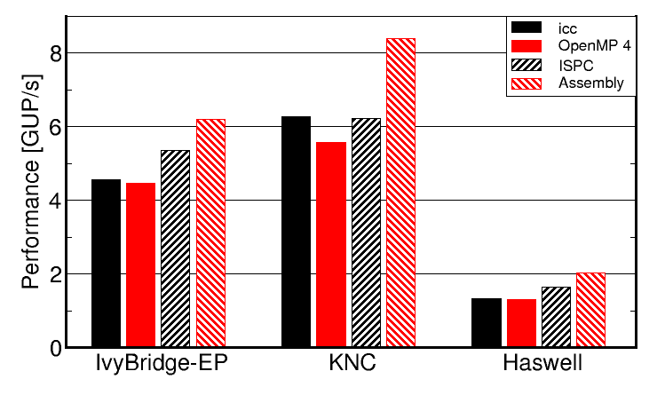
Figure 3: Performance comparison of different programming models on full systems.

Figure 3 compares our best implementations on the three platforms with compiler-generated code. We consider three different variants: C code, C code with the #pragma simd directive from the latest OpenMP 4 standard OpenMP Architecture Review Board [2013], and ISPC Pharr and Mark [2012]. The Intel C compiler version 13.1.3 with optimization flags -O3 -xHost was used on all systems. It is noteworthy that the performance using #pragma simd is worse than without the directive. ISPC (Intel SPMD Program Compiler, Version 1.5.0) is an Open Source implementation of the SPMD programming model. It provides the same performance as the Intel C compiler on KNC but on both CPUs it offers performance superior to that of the commercial Intel compiler.

The hand-written assembly kernels outperform compiler-generated code on every architecture. On IvyBridge the AVX version is 10% faster than the ISPC-generated code. The effect is more pronounced on Haswell: Because the ISPC-generated code makes use of the vector gather instruction, the hand-written assembly using pairwise loads is 22% faster. On KNC the Intel compiler provided the fastest auto-vectorized code; the hand-written IMCI version is 34% faster.

9 Conclusion

We have implemented the RabbitCT benchmark algorithm using different SIMD instruction set extensions and have benchmarked the resulting kernels on three recent Intel x86 architectures. The SIMD instruction sets exhibit different register widths ranging from 128 to 512 bits. Moreover, AVX2/FMA3 and IMCI provide instructions for vector gather and FMA. Using an instruction code analysis we have shown that it is not efficient to employ wider SIMD widths for this algorithm due to its partially scattered data access pattern. We also show that FMA and gather have a significant impact on the implementation, not only with regard to instruction count but also in terms of simplicity. By far the most compact and straightforward variant is the AVX2/FMA3 kernel. From the ISA point of view we think this is instruction code which is well suited to be automatically generated. We have then benchmarked the kernels to test the hardware implementations. The advantages at the ISA level of the gather-enabled SIMD instruction sets are currently thwarted by inefficient hardware implementations. On KNC and Haswell the current gather throughput is the dominating performance bottleneck for these kernels. An in-detail microbenchmarking analysis on these two systems revealed that the implementations suffer from significant overhead. Another issue is the fact that there is no functional latency hiding for the gather operation on KNC.

Still the new instruction sets make it easier for a compiler to generate competitive code. Therefore we think that the problem is solved on the ISA side and the vendors have to provide improved implementations to further increase the benefit of using these instructions. The advantage of GPUs for this algorithm can be explained by the bilinear interpolation being implemented completely in hardware. The second advantage is the more robust and easier to use latency hiding strategies on GPUs compared to the available multi- and many-core architectures.

We believe that RabbitCT is a very good benchmarking case to test the efficiency of available instruction sets, code generators, and microarchitectures. Future work will cover the port of our kernels on further SIMD instruction sets such as IBM VSX.

We thank IBM Research for giving Jan Treibig the opportunity for a scientific visit at the T.J.Watson Research Center, which was the starting point for this work. Special acknowledgments go to Jose Moreira for fruitful discussions.

References

- Heigl and Kowarschik [2007] B. Heigl and M. Kowarschik. High-speed reconstruction for C-arm computed tomography. In In Proceedings Fully 3D Meeting and HPIR Workshop, pages 25–28, July 2007.
- Intel Corporation [2013] Intel Corporation. Intel® 64 and IA-32 Architectures Software Developer’s Manual. Number 325462-048US. September 2013.
- Kachelriess et al. [2007] M. Kachelriess, M. Knaup, and O. Bockenbach. Hyperfast parallel-beam and cone-beam backprojection using the cell general purpose hardware. Med Phys, 34(4):1474–86, 2007. ISSN 0094-2405.
- OpenMP Architecture Review Board [2013] OpenMP Architecture Review Board. OpenMP Application Program Interface — Version 4.0. July 2013.
- Pharr and Mark [2012] M. Pharr and W. R. Mark. ispc: A SPMD Compiler for High-Performance CPU Programming. In In Proceedings Innovative Parallel Computing (InPar), San Jose, CA, May 2012.
- Pratx and Xing [2011] G. Pratx and L. Xing. Gpu computing in medical physics: A review. Medical Physics, 38(5):2685–2697, 2011. 10.1118/1.3578605. URL http://link.aip.org/link/?MPH/38/2685/1.
- Rohkohl et al. [2009] C. Rohkohl, B. Keck, H. Hofmann, and J. Hornegger. RabbitCT - an open platform for benchmarking 3D cone-beam reconstruction algorithms. Medical Physics, 36(9):3940–3944, 2009. 10.1118/1.3180956.
- Scherl et al. [2012] H. Scherl, M. Kowarschik, H. G. Hofmann, B. Keck, and J. Hornegger. Evaluation of state-of-the-art hardware architectures for fast cone-beam ct reconstruction. Parallel Comput., 38(3):111–124, Mar. 2012. ISSN 0167-8191. 10.1016/j.parco.2011.10.004. URL http://dx.doi.org/10.1016/j.parco.2011.10.004.
- Treibig et al. [2010] J. Treibig, G. Hager, and G. Wellein. LIKWID: A lightweight performance-oriented tool suite for x86 multicore environments. In PSTI2010, the First International Workshop on Parallel Software Tools and Tool Infrastructures, pages 207–216, Los Alamitos, CA, USA, 2010. IEEE Computer Society. URL http://dx.doi.org/10.1109/ICPPW.2010.38.
- Treibig et al. [2013] J. Treibig, G. Hager, H. G. Hofmann, J. Hornegger, and G. Wellein. Pushing the limits for medical image reconstruction on recent standard multicore processors. Int. J. High Perform. Comp. Appl., 27(2):162–177, 2013. 10.1177/1094342012442424.
- Zinsser and Keck [2013] T. Zinsser and B. Keck. Systematic Performance Optimization of Cone-Beam Back-Projection on the Kepler Architecture. In F. committee, editor, Proceedings of the 12th Fully Three-Dimensional Image Reconstruction in Radiology and Nuclear Medicine, page 225–228, 2013.