Observational constraints on dual intermediate inflation

Abstract

We explore the observational implications of models of intermediate inflation driven by modified dispersion relations, specifically those representing the phenomenon of dimensional reduction in the ultraviolet limit. These models are distinct from the standard ones because they do not require violations of the strong energy condition, and this is reflected in their structure formation properties. We find that they can naturally accommodate deviations from exact scale-invariance. They also make clear predictions for the running of the spectral index and tensor modes, rendering the models straightforwardly falsifiable. We discuss the observational prospects for these models and the implications these may have for quantum gravity scenarios.

I Introduction

The phenomenon of dimensional reduction in the ultraviolet (UV) energy limit has attracted a growing interest from the quantum gravity community Ambjorn et al. (2005a); Litim (2004); Lauscher and Reuter (2005a); Horava (2009a, b); Alesci and Arzano (2012); Benedetti (2009); Modesto (2009a); Caravelli and Modesto (2009); Magliaro et al. (2009); Modesto and Nicolini (2010); Calcagni (2011a, 2013). In some of these scenarios it appears that modified dispersion relations (MDRs) encode the salient features of the phenomenon Sotiriou et al. (2011). Interestingly, these modified dispersion relations may be implemented with Horava (2009a); Sotiriou et al. (2011), or without, violating the principle of relativity of inertial frames Amelino-Camelia et al. (2013a). The phenomenological implications of the deep UV limit of these MDRs can be studied by building cosmological models based upon them, and evaluating their cosmic structure formation properties Amelino-Camelia et al. (2013b) so that their predictions can be compared with observations. A minimal assumption in these calculations is that Einstein gravity (GR) is valid in the frame where the MDRs are postulated. This is called the Einstein frame. However, by disformally transforming to a frame which trivialises the MDRs, we find an equivalent dual description which displays modified gravity (more specifically ’rainbow gravity’ Magueijo and Smolin (2004)) and unmodified dispersion relations Amelino-Camelia et al. (2013c). This is called the ’rainbow frame’.

In the Einstein frame, MDRs drive cosmic structure formation Magueijo (2008a, 2009, b) without the need for inflation, but in the dual frame the cosmological expansion is perceived as accelerating. Yet, such superluminal expansion is never conventional inflation and, in particular, it is not derived from the behaviour of scalar fields or other sources of a violation of the strong energy condition. The accelerated expansion is driven purely by modified gravity Garattini and Sakellariadou (2012); Amelino-Camelia et al. (2013c) and, unsurprisingly, the conditions for a scale-invariant spectrum of density perturbations to arise are very different to those required in standard inflationary models Starobinsky (2005).

It is known that power-law MDRs lead to dual power-law and de Sitter inflation, so one may wonder what type of MDRs dualize into intermediate inflation Barrow (1990); Barrow and Saich (1990); Barrow and Liddle (1993); Barrow et al. (2006); Barrow (1995) – another example of the inflationary scenario. In Barrow and Magueijo (2013) it was shown that to achieve this style of inflation it was enough to modulate the power-law appearing in the MDRs with a logarithmic factor, typical of those arising from renormalization arguments. The purpose of this paper is to study the full observational constraints upon this model, in the light of recent observational results Ade et al. (2013). We will also study how these constraints may feed back into quantum gravity theories, and bring a much larger data set to bear upon them.

We start by presenting the model and improving the presentation in Barrow and Magueijo (2013). We shall write the MDRs, proposed in Barrow and Magueijo (2013), in the alternative form:

$$E^{2}=p^{2}\left[1+\left(\lambda p\right)^{2\gamma}\left(\frac{\ln(p_{0}/p)}{\ln(\lambda p_{0})}\right)^{2\beta}\right],$$ (1)

(valid for massless particles, but easy to adapt for massive particles) with $\beta$, $\gamma$, $\lambda$ and $p_{0}$ non-negative constants. The speed of light $c$ is obtained from the MDR via $c=dE/dp\approx E/p$. This reparameterisation has two advantages. First, it brings to the fore the fact that there is a maximum momentum $p_{\text{M}}$ in these models, as already pointed out in Barrow and Magueijo (2013). The maximum momentum is more precisely defined as the point where $c=dE/dp=0$ and this is only of the order of $p_{0}$ (for the cases we are interested in; with $\gamma$ and $\beta$ of the order of unity); specifically, $p_{\text{M}}=p_{0}\exp\left(\frac{-\beta}{1+\gamma}\right)$. Note that $p_{0}$ will always have to be a very large number, so that the cut off happens at energies higher than those needed to solve the horizon problem. This is a general feature of these models, unrelated to the issue of the fine tuning necessary for obtaining departures from scale-invariance, which is the subject of this paper.

The second advantage of parameterisation (1) concerns the logarithmic factor introduced in the denominator. With this factor, the transition between the infrared (IR) regime and the UV regime is always at $p\sim\lambda^{-1}$ (regardless of the remaining parameters). The IR regime is described then by $\lambda p\ll 1$, where the MDR turns out to be trivial as $E^{2}\approx p^{2}$, while in the UV regime, $\lambda p\gg 1$, there is a strong modification: $E^{2}\approx p^{2}\left(\lambda p\right)^{2\gamma}\left(\ln(p_{0}/p)/\ln(\lambda p_{0})\right)^{2\beta}$. This will clarify some of the points we will make regarding the spectrum normalization, and the implications for quantum gravity theories.

We highlight the specific case $\gamma=2$, known to be related to conformal invariance of the gravitational coupling Amelino-Camelia et al. (2013c) as well as to strict scale-invariance for the fluctuations. The logarithmic factor can then be seen as a soft breaker of conformal invariance. The appearance of such soft breaking is to be expected in any theory as was pointed out at the end of Amelino-Camelia et al. (2013d). Whether the resulting departure from strict scale-invariance can naturally accommodate the observations is one of the questions raised by this paper. We will argue that it can.

The plan of the rest of this paper is as follows. In section II we study the model in the context of quantum gravity, and the phenomenon of dimensional reduction in the UV regime. Specifically, we present the running spectral and Hausdorff dimensions for the most relevant case, with $\gamma=2$ and $\beta=1$. Then, in Section III we find the power spectrum for scalar and tensor perturbations in general, and focus later on the specific case $\gamma=2$. We find that for $\beta\neq 0$, this theory naturally predicts deviations from exact scale-invariance at the rough level required by observations. In Section IV, we compare the predictions with the observations in more detail, and derive constraints upon the parameters of the theory. In a concluding section we examine what the wider implications might be for quantum gravity theories.

Throughout this paper we will use Planck units (i.e. $c=\hbar=G=1$).

II Dimensional reduction associated with the MDRs

In this section we work out the dimensional reduction profile linking the IR regime and the UV regime associated with (1). We perform this using both the spectral dimension measure and the Hausdorff dimension of momentum space in a dual picture where the MDRs are trivialised, with the measure absorbing the non-trivial effects. A number of concerns have been raised regarding the use of the spectral dimension and its probabilistic interpretation Calcagni et al. (2013). These are beyond the scope of this paper, and in any case we find equivalent results whatever dimensionality measure we use, as we will now show.

II.1 The spectral dimension

The spectral dimension $d_{s}(s)$ has been proposed as a possible quantity characterising the geometry of some quantum gravity theories (Ambjorn et al. (2005b)). We can think of the spectral dimension as the effective dimension probed by a fictitious random walk process. Its average return probability at a scale $s$ is given by:

$$P(s)=\int\frac{d^{3}pdE}{(2\pi)^{4}}e^{-s\Omega_{\lambda}(p,E)},$$ (2)

where $\Omega_{\lambda}(p,E)=E^{2}+f_{\lambda}(p)$, and the defining function $f_{\lambda}(p)$ is supplied by the specific MDR. In our case, we have

$$f_{\lambda}(p)=p^{2}\left[1+(\lambda p)^{2\gamma}(\ln(p_{0}/p)/\ln(\lambda p_{0}))^{2\beta}\right].$$ (3)

We define the spectral dimension as:

$$d_{s}(s)=-2\frac{d\ln P(s)}{d\ln s}.$$ (4)

The parameter $s$ can be interpreted as the scale at which we are probing the process. For $s\rightarrow 0$ we probe the ultraviolet limit, while for $s\rightarrow\infty$ we probe the infrared. In general, the integral in (2) should consider all the possible values of the energy $E$ and momentum $p$. This means that, for our MDR, the integral of momentum must be done up to its maximum, $p_{\text{M}}$.

As has been mentioned in Amelino-Camelia et al. (2013b); Barrow and Magueijo (2013), the case of $\gamma=2$ is of special interest. This case leads to exact scale-invariance for $\beta=0$ (which describes de-Sitter spacetime in the rainbow frame), and leads to a UV spectral dimension of about $2$, which is favoured in many quantum-gravity studies (Ambjorn et al. (1998); Horava (2009c); Ambjorn et al. (2005b); Lauscher and Reuter (2005b); Kommu (2012); Giasemidis et al. (2012); Alesci and Arzano (2012); Modesto (2009b); Calcagni (2011b)). For this reason, we will study that particular case. Fig. 1 shows the result calculated for the spectral dimension $d_{s}(s)$ in the case of $\lambda=1$, $p_{0}=10^{50}$, $\gamma=2$ and $\beta=1$, in the region where the transition from UV to IR occurs.

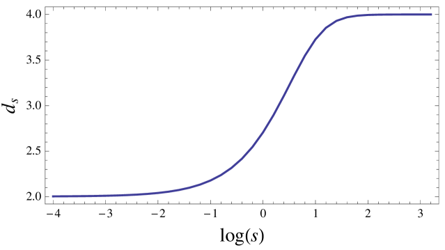
Figure 1: The transition from UV to IR of the spectral dimension, $d_{s}(s)$ for $\lambda=1$, $p_{0}=10^{50}$, $\gamma=2$ and $\beta=1$.

From Fig.1 we can see that in the IR regime, $\lim_{s\rightarrow\infty}d_{s}=4$, which is expected since eq. (1) approaches the trivial dispersion relation $E^{2}=p^{2}$ in this regime, and $d_{s}$ then coincides with the topological dimension. In addition, we can see that in the UV regime, $d_{s}$ is near to 2, which looks similar to what was found in Amelino-Camelia et al. (2013b) for $\gamma=2$ and $\beta=0$. However, Fig. 2 shows that these cases are actually different. In Amelino-Camelia et al. (2013b), it was found that $\lim_{s\rightarrow 0}d_{S}=2$, but now we observe that $d_{s}$ never settles to 2, but it keeps on increasing as $s\rightarrow 0$.

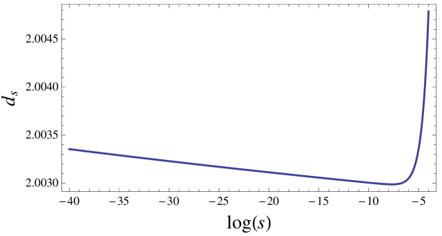
Figure 2: The UV region of the spectral dimension variation with $s$ for $\lambda=1$, $p_{0}=10^{50}$, $\gamma=2$ and $\beta=1$. Note that $d_{s}$ never settles at 2, but keeps on increasing as $s\rightarrow 0$.

II.2 The dual Hausdorff dimension

An alternative characterisation of the phenomenon of dimensional reduction was proposed in Amelino-Camelia et al. (2013d). By redefining the units of momentum it is possible to trivialise the dispersion relations. This shifts the non-trivial effects elsewhere, for example to the interactions, or to the measure of integration in momentum space. Interestingly, the latter shows a Hausdorff dimension $d_{H}$ which in the UV limit coincides with the UV spectral dimension of the theory. It was shown in Amelino-Camelia et al. (2013a) that a similar phenomenon may be found in theories which do not introduce preferred frames, but the integration measure in energy-momentum space becomes non-factorable.

In our case, trivialising the MDR can be done by defining a new (spatial) momentum variable:

$$\tilde{p}=p\left[1+(\lambda p)^{2\gamma}\left(\frac{\ln(p_{0}/p)}{\ln(\lambda p_{0})}\right)^{2\beta}\right]^{1/2}\,.$$ (5)

We can then evaluate the momentum measure $d\mu({\tilde{p}})=\mu({\tilde{p}})d\tilde{p}=p^{2}dp$, and evaluate its running Hausdorff dimension from:

$$d_{H}({\tilde{p}})=2+\frac{d\ln\mu}{d\ln\tilde{p}}.$$ (6)

Fig. 3 shows the results for the Hausdorff dimension with $\lambda=10^{4}$, $p_{0}=10^{50}$, $\gamma=2$ and $\beta=1$, during the transition from IR to UV. We observe a similar transition behaviour to that found for the spectral dimension.

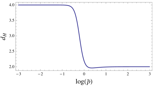
Figure 3: The transition from IR to UV of the Hausdorff dimension, $d_{H}(\tilde{p})$, of momentum space for $\lambda=1$, $p_{0}=10^{50}$, $\gamma=2$ and $\beta=1$.

In addition, Fig. 4 shows the UV region. The top plot shows the same behaviour as in the spectral dimension, where $d_{H}$ never settles to 2. However, in this case there is a maximum momentum $\tilde{p}_{\text{M}}$ (corresponding to $p_{\text{M}}$), where $d_{H}\rightarrow\infty$, as it can be seen in the bottom plot of this figure with greatly expanded scales.

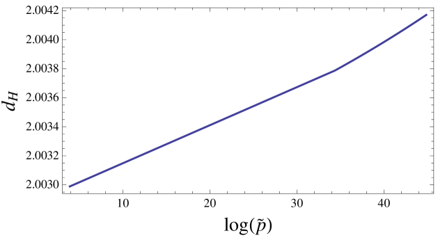
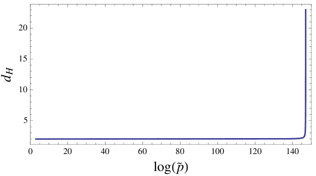
Figure 4: The UV region of the Hausdorff dimension of momentum space for $\lambda=1$, $p_{0}=10^{50}$, $\gamma=2$ and $\beta=1$. The top plot shows some UV region, where it is seen that $d_{H}$ never settles at 2, but it rather keeps on increasing. The bottom plot, with greatly expanded scales, shows the long UV regime, where a divergence is found at a maximum momentum $\tilde{p}_{M}$.

Notice that these results for the spectral and Hausdorff dimensions are general for $\gamma=2$. The specific value of $\beta$ does not affect the behaviour of $d_{s}$ nor $d_{H}$ significantly (except when $\beta=0$) because $\beta$ can only have an effect in the UV limit but in this case the polynomial term $\lambda p$ with exponent $\gamma$ dominates over the logarithmic term.

III Detailed calculation of the cosmological scalar and tensor fluctuations

MDRs models are able to produce viable primordial perturbations in the early Universe, providing an alternative to the simple models of inflation (Dodelson (2003)). This has been already shown in Amelino-Camelia et al. (2013b); Magueijo (2008b); Barrow and Magueijo (2013); Lu and Piao (2010).

In this section we calculate the scalar and tensor power spectra predicted with the MDR given by eq. (1). We will find their amplitudes along with the spectral indices, and due to the special interest in the case with $\gamma=2$, we will specialise the calculations to that case at the end.

III.1 Primordial scalar fluctuations

Let us assume that the underlying theory is GR (see Magueijo (2008b); Amelino-Camelia et al. (2013b) for the logic behind this choice) and consider the equation of motion for first-order scalar cosmological perturbations in a spatially flat Friedmann-Robertson-Walker (FRW) universe filled with a perfect fluid:

$$v^{{}^{\prime\prime}}+\left(c^{2}k^{2}-\frac{a^{{}^{\prime\prime}}}{a}\right)v=0,$$ (7)

such that $v=-\zeta/a$, and $c=E/p$ (up to a factor of order 1). We are ultimately interested in calculating the field $\zeta$, known as the curvature perturbation. The general form of this equation of motion can be found in Mukhanov et al. (1992), but we have already made some approximations given our MDR Magueijo (2008b); Amelino-Camelia et al. (2013b).

For an equation of state of matter $P=w\rho$ (with $P$ being the pressure and $\rho$ the energy density), for a spatially-flat FRW universe we have that:

$$a\propto\eta^{\frac{1}{\epsilon-1}};\quad\epsilon=\frac{3}{2}(1+w),$$ (8)

where $\eta$ is the conformal time satisfying $\eta>0$, and $w$ is assumed to be constant. In this model, the horizon problem can be solved in an expanding Universe that does not necessarily inflate, i.e. with $w>-1/3$. This is because if we take in consideration eq. (1), in the past, i.e. in the UV regime, $c$ evolves in time as:

$$c\propto\eta^{-\alpha}[C_{1}+C_{2}\ln(\eta)]^{\beta};\quad\alpha=\frac{\gamma}{\epsilon-1},$$ (9)

where $C_{1}$ and $C_{2}$ are some constants. Since we also have $a^{\prime\prime}/a\propto 1/\eta^{2}$, and we will be considering only cases where $-1/3<w<(2\gamma-1)/3$ (and therefore $\alpha>1$), then $c^{2}k^{2}\eta^{2}\ll 1$ in this regime. This means that the first term in the parenthesis of (7) dominates over the second term. Consequently, we have that in the past perturbations oscillate on sub-Hubble scales ($ck\eta\gg 1$). As time grows the second term dominates, i.e. perturbations freeze-in on super-Hubble scales ($ck\eta\ll 1$). Due to the fact that all perturbations were inside the Hubble radius during the UV regime, the horizon problem is solved.

Now, we would like to solve eq. (7), but instead of solving it exactly, we do so in two regimes: for sub-Hubble and super-Hubble scales, and then match both solutions at the horizon-crossing time. For sub-Hubble scales, the correct normalised solution is given by the WKB approximation:

$$v\approx\frac{e^{ik\int c\,d\eta}}{\sqrt{ck}}.$$ (10)

For super-Hubble scales, the solution is simply given by $v=F(k)a$, where $F(k)$ is some undetermined function. Next, we impose a continuity condition on $v$ at the horizon-crossing time $\eta_{*}$ defined by $c_{\ast}k\eta_{\ast}=1$, in order to find $F(k)$, which actually corresponds to $\zeta$ on super-Hubble scales. For simplicity, in the following calculations we will use the parametrisation of the MDR given in Barrow and Magueijo (2013):

$$E^{2}=p^{2}\left(1+(\tilde{\lambda}p)^{2\gamma}(D-\ln(\tilde{\lambda}p))^{2\beta}\right),$$ (11)

where the relation between the parameters $(D,\tilde{\lambda})$ and $(p_{0},\lambda)$ of (1) is:

$$D=\ln\left(\frac{\lambda p_{0}}{\ln(\lambda p_{0})^{\beta/2}}\right);\quad\tilde{\lambda}=\frac{\lambda}{\ln(\lambda p_{0})^{\beta/2}}.$$ (12)

By assuming that the crossing-time occurs in the UV regime, which as we will see later can be guaranteed by choosing a suitable value of $\lambda$, we can approximate $c_{\ast}\approx(\lambda p_{\ast})^{\gamma}(D-\ln(\lambda p_{\ast}))^{\beta}$ and find that the power spectrum of $\zeta$ on super-Hubble scales is:

$$\mathcal{P}_{\zeta}(k)=\frac{k^{3}}{2\pi^{2}}|\zeta|^{2}\sim\frac{\left(\tilde{\lambda}^{\gamma}D^{\beta}\right)^{\frac{\gamma-2}{\gamma+1-\epsilon}}k^{\frac{\epsilon\left(\gamma-2\right)}{\gamma+1-\epsilon}}}{2\pi^{2}\tilde{\lambda}^{\gamma}\left[E+\left(\frac{\gamma+1}{1+\gamma-\epsilon}-1\right)\ln(\tilde{\lambda}k)\right]^{\beta}},$$ (13)

such that $E\equiv D+\ln\left[\left(D^{\beta}/\tilde{\lambda}\right)^{\frac{1}{1+\gamma-\epsilon}}\right]$.

In order to see more clearly the dependence of the power spectrum on $k$, we approximate the power spectrum on some scale $k_{0}$ by

$$\mathcal{P}_{\zeta}(k)\sim A_{\zeta}^{2}\left(\frac{k}{k_{0}}\right)^{n_{\text{s}}(k_{0})-1},$$ (14)

where $A_{\zeta}^{2}=\mathcal{P}_{\zeta}(k_{0})$ is the amplitude of the power spectrum at $k_{0}$, and $n_{\text{s}}$ is the spectral index given by:

$$n_{\text{s}}(k)-1=\frac{d\ln\mathcal{P}_{\zeta}(k)}{d\ln k}$$

$$=\frac{\epsilon\left(\gamma-2\right)}{1+\gamma-\epsilon}-\frac{\beta\epsilon}{\left(1+\gamma-\epsilon\right)\left(E+\left(\frac{\gamma+1}{1+\gamma-\epsilon}-1\right)\ln(\tilde{\lambda}k)\right)}$$ (15)

Here, we can see two terms: the first comes from the polynomial part of the dispersion relation; it was already found in Magueijo (2008b), and corresponds to the particular case of $\beta=0$. The second term comes from the logarithmic part of (1) and brings a dependence on the scale $k$ into the spectral index, so the power spectrum cannot be written exactly as a purely polynomial function of $k$.

Now, we consider the specific case of $\gamma=2$. The power spectrum (13) and the spectral index (15) reduce to:

$$\mathcal{P}_{\zeta}\sim\frac{1}{2\pi^{2}\tilde{\lambda}^{2}(E+2\ln(\tilde{\lambda}k))^{\beta}};\quad E=D+\ln(D^{\beta}/\tilde{\lambda}),$$ (16)

and

$$n_{\text{s}}(k)-1=-\frac{2\beta}{E+2\ln(\tilde{\lambda}k)}.$$ (17)

Here, we have also set $\epsilon=2$ ($w=1/3$, i.e. radiation) since, as it was shown in Barrow and Magueijo (2013), in order to have a transformation from the Einstein frame with the MDR (1) to a rainbow frame with intermediate inflation and a trivial dispersion relation, we need that $\gamma=\epsilon$. In this rainbow frame, the scale factor evolves as:

$$a(t)\propto e^{At^{n}},$$ (18)

where $n$ is related to the exponents in the MDR by:

$$\beta=\frac{1}{n}-1.$$ (19)

From eq. (17) we can see that we will always have a deviation from scale-invariance as long as $\beta\neq 0$, i.e. in all the possible models of intermediate inflation. Therefore, the logarithms in eq. (1) break exact scale-invariance in the cosmological density fluctuation spectrum for $\gamma=2$.

III.2 Primordial tensor fluctuations

The equation of motion for the tensor modes, described by the field $h$, is such that if $\tilde{h}=ah$ then $\tilde{h}$ satisfies the same equation as $v$, eq. (7). Therefore, we should find the same result for $h$ as for $\zeta$. However, as was pointed out in Amelino-Camelia et al. (2013b), the MDR for gravity and for matter do not need to be the same, and consequently the expression for $c$ in the equation of motion could now be different. One simple modification of the MDR in eq. (1) could be:

$$E^{2}=p^{2}\left[1+b^{2}\left(\lambda p\right)^{2\gamma}\left(\frac{\ln(p_{0}/p)}{\ln(\lambda p_{0})}\right)^{2\beta}\right],$$ (20)

where $b$ is some dimensionless factor, whose effect is to create a constant difference in the UV regime between the speeds of gravity and light:

$$c_{\text{g}}=bc.$$ (21)

Note that this case is equivalent to having a different $\lambda$ factor for tensor perturbations. When this is the case, the power spectrum for tensor perturbations, $\mathcal{P}_{\text{T}}(k)$, at the horizon-crossing time is:

$$\mathcal{P}_{\text{T}}(k)=\left(\frac{2}{b\pi^{2}}\right)\frac{1}{\tilde{\lambda}^{2}(E+\ln(b)+2\ln(\tilde{\lambda}k))^{\beta}},$$ (22)

with a tensor spectral index given by:

$$n_{\text{T}}(k)=-\frac{2\beta}{E+2\ln(\tilde{\lambda}k)+\ln(b)};\;\mathcal{P}_{\text{T}}\sim A_{\text{T}}^{2}\left(\frac{k}{k_{0}}\right)^{n_{T}(k_{0})}.$$ (23)

Thus, the tensor-to-scalar ratio will be:

$$r=\frac{\mathcal{P}_{\text{T}}}{\mathcal{P}_{\zeta}}=\frac{4}{b}\left(1+\frac{\ln(b)}{E+2\ln(\tilde{\lambda}k)}\right)^{-\beta}.$$ (24)

The results found in this section for primordial perturbations are valid while they are frozen-in, i.e. until they re-enter the horizon again. Since for a given comoving momentum, $k$, the end of the varying-$c$ period ($\lambda p\sim 1$) happens when $ck\eta\sim k^{2}\lambda$ (ignoring the matter epoch for simplicity, and defining $a=1$ today), then for all cosmologically relevant scales we have a set of suitable $\lambda$ values such that $k^{2}\lambda\ll 1$, i.e. the speed of light becomes constant while the perturbations are on super-Hubble scales. This means that perturbations will re-enter the horizon when $c=1$, which lets us compare our results to the observational ones. In addition, this also means that perturbations crossed the horizon for the first time during the UV regime, as we assumed in the previous calculations.

IV Observational constraints when $\boldsymbol{\gamma=2}$

We can now compare our predictions for $\gamma=2$ to the observational results found in Ade et al. (2013). In the case of the scalar power spectrum, for the form written in eq. (14), in this reference, it was found that for $k_{0}=0.05Mpc^{-1}$:

$$A_{\zeta}^{2} =\left(2.196_{-0.060}^{+0.051}\right)\times 10^{-9},$$ (25)

$$n_{\text{s}}-1 =-0.0371\pm 0.0057.$$ (26)

These values constrain the set of parameters $(\beta,p_{0},\lambda)$ of our model. It is convenient to study the case where $p_{0}$ is fixed due to the fact that $p_{0}$ always appears as $\ln(p_{0})$ in eqs. (16) and (17), and then these observational constraints will predict a big uncertainty for this parameter. If we do this, then the observations at $k_{0}$ constrain the parameters $\beta$ and $\lambda$. For the case of $p_{0}=10^{135}$, the results are shown in Fig. 5.

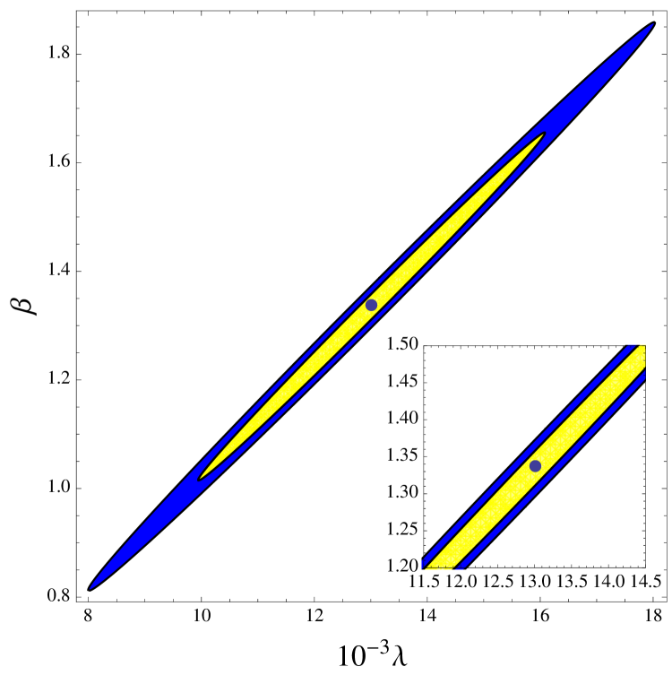
Figure 5: The two-parameter $(\beta,\lambda)$ joint error bounds for $p_{0}=10^{135}$ and $\gamma=2$ imposed by the Planck scalar spectrum bounds Ade et al. (2013). The yellow and blue ellipses represent the expected constraint on the parameter space with $1\sigma$ and $2\sigma$ significance, respectively.

Fig. 5 shows the $(\beta,\lambda)$ joint error bounds. The dot in the plot shows the set $(\bar{\beta}=1.3353,\bar{\lambda}=1.3013\times 10^{4})$ that maximises the likelihood, i.e. that give the observational central values in eqs. (25)-(26), when replaced in the theoretical equations (16) and (17), for $p_{0}=10^{135}$. Using the Fisher matrix technique, we find the approximated regions with $1\sigma$ and $2\sigma$ joint errors, represented by the yellow and blue regions, respectively. We observe that both parameters are highly correlated, in fact $Corr(\lambda,\beta)=99.7\%$. The errors found yield $\lambda=(1.3013\pm 0.2020)\times 10^{4}$ and $\beta=1.3353\pm 0.2108$.

Since our model predicts a $k$-dependent spectral index at next order, we could improve our approximation of the power spectrum by expanding $\mathcal{P}_{\zeta}$ as:

$$\mathcal{P}_{\zeta}(k)\sim A_{\zeta}^{2}\left(\frac{k}{k_{0}}\right)^{n_{\text{s}}(k_{0})-1+\frac{1}{2}\ln(k/k_{0})\alpha+\frac{1}{6}\ln^{2}(k/k_{0})\alpha_{2}},$$ (27)

where, at some pivotal scale $k_{0}$, the index $n_{\text{s}}$ is given by eq. (17), while $\alpha$ and $\alpha_{2}$ are given by:

$$\alpha\equiv\left.\frac{dn_{\text{s}}}{d\ln(k)}\right|_{k_{0}}=\frac{4\beta}{\left(E+2\ln(\tilde{\lambda}k_{0})\right)^{2}},$$ (28)

$$\alpha_{2}\equiv\left.\frac{d^{2}n_{\text{s}}}{d\ln k^{2}}\right|_{k_{0}}=\frac{-16\beta}{\left(E+2\ln(\tilde{\lambda}k_{0})\right)^{3}}.$$ (29)

In Ade et al. (2013) it was found that, for $k_{0}=0.05Mpc^{-1}$, the constraints are:

$$n_{\text{s}}-1 =-0.0432_{-0.0063}^{+0.0068},$$ (30)

$$\alpha =0.000_{-0.013}^{+0.016},$$ (31)

$$\alpha_{2} =0.017_{-0.014}^{+0.016},$$ (32)

while $A_{\zeta}^{2}$ is given by eq. (25). Again, these values constrain the set of parameters $(\beta,p_{0},\lambda)$ of our model. Fig. 6 shows a sample of the set of parameters that give the central observational values of (25) and (30).

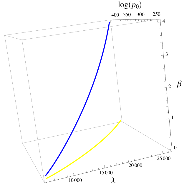
Figure 6: The set of values for $(\beta,\lambda,\log(p_{0}))$ satisfying the experimental constraints of $A_{\zeta}^{2}$, and $n_{\text{s}}$ at $k_{0}=0.05Mpc^{-1}$, represented by the blue line. We also show the projection of this line onto the $(\lambda,\log(p_{0}))$ plane, represented by the yellow line.

In Fig. 6 we draw a 3-dimensional box with axes $(\beta,\log(p_{0}),\lambda)$. The blue line shows the concordant set of parameters while the yellow line is its projection onto the plane $(0,\log(p_{0}),\beta)$. Here, we only plot a sample range of parameters such that $\beta$ is in the range of $0.1\leqslant\beta\leqslant 4$.

Not all of parameter values in the set shown in Fig. 6 satisfy the observational central values found for $\alpha$ and $\alpha_{2}$ in ref.Ade et al. (2013). In the case of $\alpha$, we can calculate the predicted values by using the set of parameters in Fig. 6 and eq. (28). This set of predicted values for $\alpha$ will always have positive values and therefore they will have some deviation from the central observed value $\bar{\alpha}=0$. Fig. 7 shows this deviation (in terms of the error $\sigma(\alpha)=0.016$) as a function of the parameter $\beta$. In this figure we see that the deviation is less than $1.2\sigma(\alpha)$ for the sampled values of $\beta$.

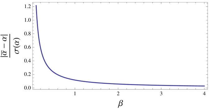
Figure 7: The deviation of $\alpha$ (in terms of the error $\sigma(\alpha)$) from the central experimental value of $\alpha$ from ref. Ade et al. (2013) as a function of $\beta$.

On the other hand, in the case of $\alpha_{2}$ we notice that, observationally, it is expected to be positive at a level of about $1.2\sigma(\alpha_{2})$ (see eq. (32)), where $\sigma(\alpha_{2})=0.014$. However, our theory always predicts a negative value, as eq. (29) shows . If now we do the same study we just did for $\alpha$, we will always predict values with a deviation of more than $1\sigma(\alpha_{2})$, as shown in Fig. 8. From this plot we can see that the deviation of $\alpha_{2}$ is less than $2.5\sigma$ for the set of sampled $\beta$ values.

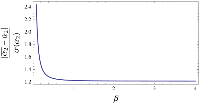
Figure 8: The deviation of $\alpha_{2}$ (in terms of the error $\sigma(\alpha_{2})$) from the central observational value of $\alpha_{2}$ as a function of $\beta$.

Therefore, even though there are predicted deviations from the central values of $\alpha$ and $\alpha_{2}$, these do not rule out the model because they are sufficiently small.

On the other hand, we could also find the appropriate value for the parameter $b$ which sets the tensor-to-scalar ratio. In Ade et al. (2013) a maximum value of

$$r<0.12$$ (33)

was found at the pivotal scale $k_{0}=0.002Mpc^{-1}$. The corresponding condition on the parameter $b$ will depend on the values we take for $(D,\tilde{\lambda},\beta)$ (or, equivalently for the set $(p_{0},\lambda,\beta)$). For the case with a fixed $p_{0}=10^{135}$, and the values $(\bar{\lambda},\bar{\beta})$, we must have $b>31.3$ in order to satisfy the lower limit on $r$. This means that in the high-energy regime, the speed of gravity exceeds the speed of light. We could also contemplate scenarios where the parameter $\beta$ is different for the scalar and tensor case, so we would have separate $\beta_{\text{s}}$ and $\beta_{\text{T}}$ parameters with different values.

V Conclusions

We have studied the cosmological implications of a specific class of MDRs, when they are combined with general relativity to create an early Universe cosmology. The resulting cosmology is equivalent to a dual model displaying intermediate inflation driven by modified gravity, in the guise of rainbow gravity. The specific case $\gamma=2$ is very interesting both from the quantum gravitational and the cosmological perspectives. When $\beta=0$ the MDRs are known to model the running from four dimensions in the IR to two dimensions in the UV (Amelino-Camelia et al. (2013b)), as suggested by numerous quantum gravity studies (Ambjorn et al. (1998); Horava (2009c); Ambjorn et al. (2005b); Lauscher and Reuter (2005b); Kommu (2012); Giasemidis et al. (2012); Alesci and Arzano (2012); Modesto (2009b); Calcagni (2011b)). The associated cosmological model then predicts exact scale-invariance for the primordial fluctuations. If we resort to fractional powers, with $\gamma$ slightly larger than 2, it is possible, but contrived, to produce departures from exact scale-invariance. Keeping $\gamma=2$, but building in a very long UV transient (as suggested in Amelino-Camelia et al. (2013b)) , is a more contrived possibility. The MDRs associated with intermediate inflation resolve this problem. Using both the spectral and Hausdorff dimension, we found that when $\gamma=2$ but $\beta\neq 0$, after an apparent running from 4 to 2 dimensions at the scale $\lambda$, the dimension never settles at 2, but drifts upwards very slowly over several orders of magnitude in energy. This can be achieved with natural values for $\beta$, say 1 or 2. This phenomenon would be hard to measure in simulations (e.g. in Causal Dynamical Triangulations, abbreviated as CDTs) without the development of specific methods. And yet the logarithmic corrections in the MDRs are typical of renormalisation group corrections. From the observational point of view this is precisely what supplies a natural mechanism for inducing departures from scale invariance in the primordial power spectrum, as we explicitly confirmed with calculations of the expected perturbations.

We studied the cosmological observational implications of this model in detail. We found that the model is able to predict primordial fluctuations in accordance with observations, in an expanding (but not inflating) early Universe dominated by radiation. Specifically, setting $\gamma=2$ and $P/\rho\equiv w=1/3$, we showed that a considerable range of the remaining model parameters can lead to viable predictions for the resulting cosmological density perturbations. We find that $\beta$ does not need to be highly contrived, since it can be at least in the range 1-5, while the length scale $\lambda$ must be four orders of magnitude above the Planck scale in order to obtain $n_{S}\sim 0.96$ and explain the amplitude $A_{\zeta}$. In addition, we introduced a new parameter in the theory to model tensor perturbations, which is capable of explaining the observed upper bound of the tensor-to-scalar ratio. The parameter choices made in this model can be compared with those typically made to arrive at best-fit inflationary models Ade et al. (2013).

Our model makes clear prediction for the running of the spectral index, encoded in eq. (28) and (29). These may go against current observational “trends” (e.g. in terms of sign for one of these parameters), but typically at only around $1\sigma$ (and never by more than $2.5\sigma$ in the range of parameters considered). This explains our label “trends” for these observations, which are not discriminating enough for the purpose of the model proposed here. However, this very remark leaves open the prospect of falsifying or verifying these models, as the data sharpens and becomes more discriminating. The running of the spectral index could be the ideal test for this class of models.

On the other hand, predictions based on non-Gaussianity (e.g. $f_{NL}$) remain to be worked out. We emphasise that we cannot simply read off the results obtained for single field intermediate inflation (Chen (2010)). A rather non-trivial fresh calculation is needed, since we would have to calculate the third-order action for higher-order derivative theories. This will be the subject of a future paper.

We close by noting that the models considered here are among the simplest of those leading to rainbow intermediate inflation. By fixing $\gamma=2$ we are requiring that in the Einstein frame the Universe be filled with radiation, i.e. $w=1/3$ (cf. eq. (27) in Barrow and Magueijo (2013)). In the rainbow frame, a case of interest is $\beta=1$, where we have that the scale factor evolves as:

$$a\left(\tilde{t}\right)\propto\lambda k\exp{\left(\frac{a_{0}\tilde{t}^{1/2}}{\lambda k}\right)}\;,$$ (34)

where here we have used some notation defined in Barrow and Magueijo (2013). These models softly break the conformal invariance of the gravitational coupling of fluctuations, which is peculiar to these models when $\beta=0$ as it was shown in Amelino-Camelia et al. (2013c). This is the root of their phenomenological and theoretical interest as alternatives to inflation for a detailed explanation of the structure observed in the cosmic microwave background radiation.

References

- Ambjorn et al. (2005a) J. Ambjorn, J. Jurkiewicz, and R. Loll, Phys.Rev.Lett. 95, 171301 (2005a), arXiv:hep-th/0505113 [hep-th] .
- Litim (2004) D. F. Litim, Phys.Rev.Lett. 92, 201301 (2004), arXiv:hep-th/0312114 [hep-th] .
- Lauscher and Reuter (2005a) O. Lauscher and M. Reuter, JHEP 0510, 050 (2005a), arXiv:hep-th/0508202 [hep-th] .
- Horava (2009a) P. Horava, Phys.Rev. D79, 084008 (2009a), arXiv:0901.3775 [hep-th] .
- Horava (2009b) P. Horava, Phys.Rev.Lett. 102, 161301 (2009b), arXiv:0902.3657 [hep-th] .
- Alesci and Arzano (2012) E. Alesci and M. Arzano, Phys.Lett. B707, 272 (2012), arXiv:1108.1507 [gr-qc] .
- Benedetti (2009) D. Benedetti, Phys.Rev.Lett. 102, 111303 (2009), arXiv:0811.1396 [hep-th] .
- Modesto (2009a) L. Modesto, Class.Quant.Grav. 26, 242002 (2009a), arXiv:0812.2214 [gr-qc] .
- Caravelli and Modesto (2009) F. Caravelli and L. Modesto, (2009), arXiv:0905.2170 [gr-qc] .
- Magliaro et al. (2009) E. Magliaro, C. Perini, and L. Modesto, (2009), arXiv:0911.0437 [gr-qc] .
- Modesto and Nicolini (2010) L. Modesto and P. Nicolini, Phys.Rev. D81, 104040 (2010), arXiv:0912.0220 [hep-th] .
- Calcagni (2011a) G. Calcagni, Phys.Lett. B697, 251 (2011a), arXiv:1012.1244 [hep-th] .
- Calcagni (2013) G. Calcagni, Phys.Rev. E87, 012123 (2013), arXiv:1205.5046 [hep-th] .
- Sotiriou et al. (2011) T. P. Sotiriou, M. Visser, and S. Weinfurtner, Phys.Rev. D84, 104018 (2011), arXiv:1105.6098 [hep-th] .
- Amelino-Camelia et al. (2013a) G. Amelino-Camelia, M. Arzano, G. Gubitosi, and J. Magueijo, (2013a), arXiv:1311.3135 [gr-qc] .
- Amelino-Camelia et al. (2013b) G. Amelino-Camelia, M. Arzano, G. Gubitosi, and J. Magueijo, Phys. Rev. D 87, 123532 (2013b), 1305.3153 .
- Magueijo and Smolin (2004) J. Magueijo and L. Smolin, Class. Quant. Grav. 21, 1725 (2004), arXiv:gr-qc/0305055 .
- Amelino-Camelia et al. (2013c) G. Amelino-Camelia, M. Arzano, G. Gubitosi, and J. Magueijo, Phys. Rev. D 88, 041303 (2013c), 1307.0745 .
- Magueijo (2008a) J. Magueijo, Phys.Rev.Lett. 100, 231302 (2008a), arXiv:arXiv:0803.0859 [astro-ph] .
- Magueijo (2009) J. Magueijo, Phys.Rev. D79, 043525 (2009), arXiv:0807.1689 [gr-qc] .
- Magueijo (2008b) J. Magueijo, Class.Quant.Grav. 25, 202002 (2008b), arXiv:0807.1854 [gr-qc] .
- Garattini and Sakellariadou (2012) R. Garattini and M. Sakellariadou, (2012), arXiv:1212.4987 [gr-qc] .
- Starobinsky (2005) A. A. Starobinsky, JETP Lett. 82, 169 (2005), arXiv:astro-ph/0507193 [astro-ph] .
- Barrow (1990) J. D. Barrow, Phys.Lett. B235, 40 (1990).
- Barrow and Saich (1990) J. D. Barrow and P. Saich, Phys.Lett. B249, 406 (1990).
- Barrow and Liddle (1993) J. D. Barrow and A. R. Liddle, Phys.Rev. D47, 5219 (1993), arXiv:astro-ph/9303011 [astro-ph] .
- Barrow et al. (2006) J. D. Barrow, A. R. Liddle, and C. Pahud, Phys.Rev. D74, 127305 (2006), arXiv:astro-ph/0610807 [astro-ph] .
- Barrow (1995) J. D. Barrow, Phys.Rev. D51, 2729 (1995).
- Barrow and Magueijo (2013) J. D. Barrow and J. Magueijo, Phys. Rev. D 88, 103525 (2013), arXiv:1310.2072 [astro-ph.CO] .
- Ade et al. (2013) P. Ade et al. (Planck Collaboration), (2013), arXiv:1303.5076 [astro-ph.CO] .
- Amelino-Camelia et al. (2013d) G. Amelino-Camelia, M. Arzano, G. Gubitosi, and J. Magueijo, (2013d), arXiv:1309.3999 [gr-qc] .
- Calcagni et al. (2013) G. Calcagni, A. Eichhorn, and F. Saueressig, Phys.Rev. D87, 124028 (2013), arXiv:1304.7247 [hep-th] .
- Ambjorn et al. (2005b) J. Ambjorn, J. Jurkiewicz, and R. Loll, Phys.Rev.Lett. 95, 171301 (2005b), arXiv:hep-th/0505113 [hep-th] .
- Ambjorn et al. (1998) J. Ambjorn, D. Boulatov, J. L. Nielsen, J. Rolf, and Y. Watabiki, JHEP 9802, 010 (1998), arXiv:hep-th/9801099 [hep-th] .
- Horava (2009c) P. Horava, Phys.Rev.Lett. 102, 161301 (2009c), arXiv:0902.3657 [hep-th] .
- Lauscher and Reuter (2005b) O. Lauscher and M. Reuter, JHEP 0510, 050 (2005b), arXiv:hep-th/0508202 [hep-th] .
- Kommu (2012) R. Kommu, Class.Quant.Grav. 29, 105003 (2012), arXiv:1110.6875 [gr-qc] .
- Giasemidis et al. (2012) G. Giasemidis, J. F. Wheater, and S. Zohren, J.Phys. A45, 355001 (2012), arXiv:1202.6322 [hep-th] .
- Modesto (2009b) L. Modesto, Class.Quant.Grav. 26, 242002 (2009b), arXiv:0812.2214 [gr-qc] .
- Calcagni (2011b) G. Calcagni, Phys.Lett. B697, 251 (2011b), arXiv:1012.1244 [hep-th] .
- Dodelson (2003) S. Dodelson, Modern Cosmology (Academic Press, Elsevier Science, 2003).
- Lu and Piao (2010) Y. Lu and Y.-S. Piao, Int.J.Mod.Phys. D19, 1905 (2010), arXiv:0907.3982 [hep-th] .
- Mukhanov et al. (1992) V. F. Mukhanov, H. A. Feldman, and R. H. Brandenberger, Phys.Rep. 215, 203 (1992).
- Chen (2010) X. Chen, Adv.Astron. 2010, 638979 (2010), arXiv:1002.1416 [astro-ph.CO] .