Distance to boundary and minimum-error discrimination

Abstract

We introduce the concept of boundariness capturing the most efficient way of expressing a given element of a convex set as a probability mixture of its boundary elements. In other words, this number measures (without the need of any explicit topology) how far the given element is from the boundary. It is shown that one of the elements from the boundary can be always chosen to be an extremal element. We focus on evaluation of this quantity for quantum sets of states, channels and observables. We show that boundariness is intimately related to (semi)norms that provide an operational interpretation of this quantity. In particular, the minimum error probability for discrimination of a pair of quantum devices is lower bounded by the boundariness of each of them. We proved that for states and observables this bound is saturated and conjectured this feature for channels. The boundariness is zero for infinite-dimensional quantum objects as in this case all the elements are boundary elements.

I Introduction

The experimetal ability to switch randomly between physical apparatuses of the same type naturally endows mathematical representatives of physical objects with a convex structure. This makes the convexity (and intimately related concept of probability) one of the key mathematical features of any physical theory. Even more, the particular “convexity flavor” plays a crucial role in the differences not only between the types of physical objects, but also between the theories. For example, the existence of non-unique convex decomposition of density operators is the property distinguishing quantum theory from the classical one Holevo .

Our goal is to study the convex structures that naturally appear in the quantum theory and to illustrate the operational meaning of the concepts directly linked to the convex structure. However, most of our findings are applicable for any convex set. The main goal of this paper is to introduce and investigate the concept of boundariness quantifying how far the individual elements of the convex set are from its boundary. Intuitively, the boundariness determines the most non-uniform (binary) convex decomposition into boundary elements, hence, it quantifies how mixed the element is. We will show that this concept is operationally related to specification of the most distinguishable element (in a sense of minimum-error discrimination probability). For instance, for states the evaluation of boundariness coincides with the specification of the best distinghuishable state from the given one, hence it is proportional to trace-distance Helstrom .

The paper is organized as follows: Section II introduces the concept of boundariness and related results in general convex sets, the boundariness for quantum sets is evaluated in Section III and the relation to minimum-error discrimination is described in Section IV. Section V shortly summarizes the main results. The appendices contain mathematical details concerning the properties of weight function, characterization of the boundary elements of all considered quantum sets and numerical details of the case study.

II Convex structure and boundariness

In any convex set $Z$ we may define a convex preorder $\leq_{C}$. We say $x\leq_{C}y$ if $x$ may appear in the convex decomposition of $y$ with a non zero weight, i.e. there exist $z\in Z$ such that $y=tx+(1-t)z$ with $0<t\leq 1$. If $x\leq_{C}y$, then $y$ has $x$ in its convex decomposition, hence, (losely speaking) $y$ is “more” mixed than $x$. The value of $t$ (optimized over $z$) can be used to quantify this relation. Namely, for any element $y\in Z$ we define the weight function $t_{y}:Z\to[0,1]$ assigning for every $x\in Z$ the supremum of possible weights $t$ of the point $x$ in the convex decomposition of $y$, i.e.

$$t_{y}(x)=\sup\Big{\{}0\leq t<1\,\Big{|}\,z=\frac{y-tx}{1-t}\in Z\Big{\}}\,.$$

Obviously, $t_{y}(y)=1$ and $t_{y}(x)=0$ whenever $x\nleq_{C}y$. In order to understand the geometry of the optimal $z$ for a given pair of elements $x,y$, it is useful to express the element $z$ in the form $z=y+\frac{t}{1-t}(y-x)$. As $t$ increases, $z$ moves in the direction of $y-x$ until (for value $t=t_{y}(x)$) it leaves the set $Z$ (see Fig. 1 for illustration). If the element $z$ associated with $t_{y}(x)$ is an element of $Z$, then it can be identified as a boundary element of $Z$.

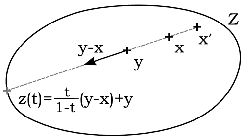
Figure 1: Illustration of elements $z$ and $x^{\prime}$ emerging in the definition of the weight function $t_{y}(x)$ and in the property $t_{y}(x^{\prime})\leq t_{y}(x)$, respectively.

The (algebraic) boundary $\partial Z$ contains all elements $y$ for which there exists $x$ such that $x\nleq_{C}y$ (let us stress this is equivalent with the definition used in Ref. dlp ). Hence, for each boundary element $y$ the weight function $t_{y}(x)=0$ for some $x$ and also the opposite claim holds, i.e., if there exists $x\in Z:t_{y}(x)=0$ then $y\in\partial Z$. As a consequence, $t_{y}(x)>0$ $\forall x\in Z$ for all inner points $y\in Z\setminus\partial Z$.

This motivates the following definition of boundariness

$$b(y)=\inf_{x\in Z}t_{y}(x)$$

measuring how far the given element of $Z$ is from the boundary $\partial Z$. Suppose $x^{\prime}$ belongs to the line generated by $x$ and $y$, i.e. $x^{\prime}=y-k(y-x)$ ($x^{\prime}=x$ for $k=1$ and $x^{\prime}=y$ for $k=0$). Then $t_{y}(x^{\prime})\leq t_{y}(x)$ whenever $k\geq 1$ (see Fig. 1). Hence, the infimum can be approximated again by some boundary element of $Z$. In other words, the value of boundariness is determined by the most non-uniform convex decomposition of $y$ into boundary elements of $Z$, i.e. $y$ can be, in a sense, approximated by expressions $b(y)x+(1-b(y))z$ with $x,z\in\partial Z$. Therefore, $b(y)\leq 1/2$. See Fig. 2 for illustration of boundariness for simple convex sets.

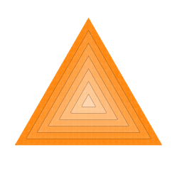
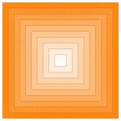
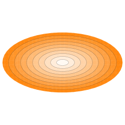
Figure 2: (Color online) Contour plots of boundariness for simple convex sets. Let us note that the maximal value of boundariness is not the same in all of them.

Lemma 1

Let $y\in Z$. The inverse $x\mapsto 1/t_{y}(x)$ of the weight function $t_{y}$ is convex, i.e.,

$$\frac{1}{t_{y}\big{(}sx_{1}+(1-s)x_{2}\big{)}}\leq\frac{s}{t_{y}(x_{1})}+\frac{1-s}{t_{y}(x_{2})}$$

for all $x_{1},\,x_{2}\leq_{C}y$ and $0\leq s\leq 1$.

Proof. For every $0<t_{i}<t_{y}(x_{i})$ $i=1,2$ we define $z_{i}=y-\frac{t_{i}}{1-t_{i}}(x_{i}-y)\in Z$. Further, we define $x=sx_{1}+(1-s)x_{2}$ and $z=uz_{1}+(1-u)z_{2}$, where $x,\,z\in Z$ because $s\in[0,1]$ and

$$u=\frac{s\frac{1-t_{1}}{t_{1}}}{s\frac{1-t_{1}}{t_{1}}+(1-s)\frac{1-t_{2}}{t_{2}}}\;\in[0,1].$$ (1)

See Fig. 3 for illustration. Straightforward calculation shows that we may write $y=tx+(1-t)z$, where $t^{-1}=st_{1}^{-1}+(1-s)t_{2}^{-1}$. From the definition of the weight function, we have $t\leq t_{y}(x)$. Since this holds for all $0<t_{i}<t_{y}(x_{i})$ $i=1,2$ we get $(\frac{s}{t_{y}(x_{1})}+\frac{1-s}{t_{y}(x_{2})})^{-1}\leq t_{y}(x)$, which concludes the proof. $\,\blacksquare$

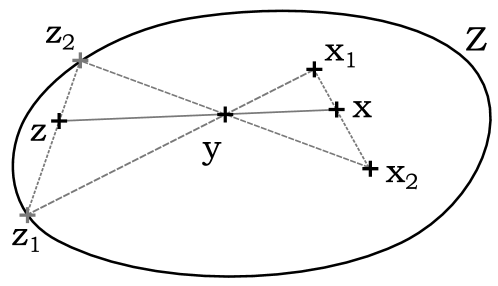
Figure 3: Illustration of the proof of the Lemma 1

The following proposition is one of the key results of this section. It guarantees that one of the elements of the optimal decomposition (determining the boundariness) can be chosen to be an extreme point of $Z$. It is shown in Appendix A that, whenever $Z\subset\mathbb{R}^{n}$ for some $n\in\mathbb{N}$, the weight function $t_{y}$ is continuous if (and only if) $y\in Z\setminus\partial Z$. Continuity of $t_{y}$ is studied in the appendices also in a slightly more general context.

Proposition 1

Suppose that $Z\subset\mathbb{R}^{n}$ is convex and compact set. For every $y\in Z\setminus\partial Z$ there exists an extreme point $x\in Z$ such that $b(y)=t_{y}(x)$.

Proof. The continuity implies that $t_{y}$ acquires its lowest value on the compact set $Z$, i.e., $b(y)=\inf_{x\in Z}t_{y}(x)=\min_{x\in Z}t_{y}(x)$. Since $y\in Z\setminus\partial Z$, we have $t_{y}(x)>0$. Moreover, because of the convexity of $x\mapsto 1/t_{y}(x)$ proven in Lemma 1, it follows that

$$\min_{x\in Z}t_{y}(x) = \big{(}\max_{x\in Z}1/t_{y}(x)\big{)}^{-1}$$

$$= \big{(}\max_{x\in\mathrm{ext}\,Z}1/t_{y}(x)\big{)}^{-1}=\min_{x\in\mathrm{ext}\,Z}t_{y}(x)\,,$$

where $\mathrm{ext}\,Z$ denotes the set of extreme points of $Z$. $\,\blacksquare$

The convex sets appearing in quantum theory are typically compact and convex subsets of $\mathbb{R}^{n}$, meaning that the above proposition is applicable in our subsequent analysis. It is easy to show that, in the context of Proposition 1, for any $y\in Z\setminus\partial Z$ and $x\in Z$ there exists an element $z\in\partial Z$ such that $y=t_{y}(x)x+\big{(}1-t_{y}(x)\big{)}z$. This, combined with Proposition 1, yields that for any $y\in Z\setminus\partial Z$ there is $x\in\mathrm{ext}\,Z$ and $z\in\partial Z$ such that $y=b(y)x+\big{(}1-b(y)\big{)}z$ when $Z$ is a convex and compact subset of $\mathbb{R}^{n}$.

Suppose that $y\in Z\setminus\partial Z$, where $Z\subset\mathbb{R}^{n}$ is a convex and compact set. Let $x\in\mathrm{ext}\,Z$ be an element, whose existence is guaranteed by Proposition 1, such that $b(y)=t_{y}(x)$. If one had $b(y)=0$, this would mean that $t_{y}(x)=0$ implying that $x$ does not appear in any convex decomposition of $y$. This yields the counterfactual result $y\in\partial Z$. Hence, $b(y)>0$ for any non-boundary element $y\in Z$, and we see that, in the context of Proposition 1, $b(y)=0$ if and only if $y\in\partial Z$. Compactness is an essential requirement for this property. Consider, e.g., a convex set $Z\subset\mathbb{R}^{n}$ that has a direction, i.e., there is a vector $v\in\mathbb{R}^{n}$ and a point $y\in Z\setminus\partial Z$ such that $y+\alpha v\in Z$ for all $\alpha>0$. Such set is not compact and one easily sees that $b(y)=0$.

Remark 1

(Evaluation of boundariness)
In practise, it is useful to think about some numerical way how to evaluate the boundariness. It follows from the definition of boundariness that for any element $y\in Z$ written as a convex combination $y=tx+(1-t)z$ with $z\in\partial Z$ the value of $t$ (being $t_{y}(x)$ in this case) provides an upper bound on the boundariness, hence $t\equiv t_{y}(x)\geq b(y)$. Suppose we are given $y$ and choose some value of $t$. Recall that for a fixed $y\in Z$ and for every $x\in Z$ the element $z_{t}(x)=(y-tx)/(1-t)$ leaves the set $Z$ for $t=t_{y}(x)$. Therefore, if we choose $t\leq b(y)$ implying $t\leq t_{y}(x)$, then $z_{t}(x)\in Z$ for all $x\in Z$. However, if it happens that $t>b(y)$, then for some $x$ we find $t>t_{y}(x)$ and consequently $z_{t}(x)\notin Z$. Even more, according to Proposition 1 such $x$ (determining the element $z_{t}(x)$ out of $Z$) can be chosen to be extremal. In conclusion, if $t>b(y)$, then there exist $x\in\mathrm{ext}Z$ such that $z_{t}(x)=(y-tx)/(1-t)\notin Z$.

This observation provides the basics of the numerical method we used to test whether a given value of $t$ coincide with $b(y)$, or not. In particular, for any $y$ we start with the maximal value of $t=1/2$ (if we do not have a better estimate) and decrease it until we reach the value of $t$ for which $z_{t}(x)\in Z$ for all $x\in\mathrm{ext}Z$. Equivalently, we may start with $t=0$ and increase its value until we find $t$ for which $z_{t+\varepsilon}(x)\notin Z$ for some $x\in\mathrm{ext}Z$ and $\forall\varepsilon>0$.

In what follows we will formulate a proposition that related relates the value of boundariness to any (bounded) seminorm defined on the (real) vector space $V$ containing the convex set $Z$.

Proposition 2

Consider a (semi)norm $p:V\to[0,\infty)$ such that $p(x)\leq a$ for all $x\in Z$ with some $a\geq 0$. Then

$$p(x-y)\leq 2a\big{(}1-t_{y}(x)\big{)}\leq 2a\big{(}1-b(y)\big{)}$$ (2)

for all $x,\,y\in Z$.

Proof. Pick $x,\,y\in Z$. The last inequality in (2) follows immediately from the definition of boundariness so we concentrate on the first inequality. If $t_{y}(x)=0$ then the claim is trivial and follows from the triangle inequality for the seminorm. Let us assume that $t_{y}(x)>0$ and pick $t\in[0,t_{y}(x))$. According to the definition of the weight function, we have $z(t)=(1-t)^{-1}(y-tx)\in Z$. It follows that $x-y=(1-t)\big{(}x-z(t)\big{)}$ yielding

$$p(x-y) = (1-t)p\big{(}x-z(t)\big{)}\leq(1-t)\big{(}p(x)+p\big{(}z(t)\big{)}\big{)}$$

$$\leq 2a(1-t).$$

As we let $t$ to approach $t_{y}(x)$ from below, we obtain the first inequality of (2). $\,\blacksquare$

In Section IV we will employ this proposition to relate the concept of boundariness to error rate of minimum-error discrimination in case of quantum convex sets of states, channels and observables. Shortly, the optimal values of error probabilities are associated with the so-called base norms jencova2013 ; reeb_etal2011 , thus setting $p(x-y)=\|x-y\|_{Z}$ in Eq. (2) we obtain an operational meaning of boundariness. Let us stress that the base norm $\|x-y\|_{Z}$ can be introduced only if certain conditions are met.

In particular, let us assume that the real vector space $V$ is equipped with a cone $C\subset V$, i.e., $C$ is a convex set such that $\alpha v\in C$ for any $v\in C$ and $\alpha\geq 0$. Moreover, we assume that $C$ is pointed, i.e., $C\cap(-C)=\{0\}$ and generating, i.e., $C-C=V$. Further, suppose $Z\subset C$ is a base for $C$, i.e., $Z$ is convex and for any $v\in C$ there are unique $x\in Z$ and $\alpha\geq 0$ with $v=\alpha x$. Especially when $x\in Z$, there is no non-negative factor $\alpha\neq 1$ such that $\alpha x\in Z$. Moreover, it follows that $0\notin Z$.

Let us note that all quantum convex sets are bases for generating cones for their ambient spaces. For example, the set of density operators $\mathcal{S}(\mathcal{H})$ on a Hilbert space $\mathcal{H}$ is the base for the cone of positive trace-class operators which, in turn, generates the real vector space of selfadjoint trace-class operators. This is the natural ambient space for $\mathcal{S}(\mathcal{H})$ rather than the entire space of selfadjoint bounded operators, although the value for the boundariness of an individual state does not change if the considered ambient space is larger than the space of selfadjoint trace-class operators.

Whenever $Z$ is a base of a generating cone in $V$ one can define the base norm $\|\cdot\|_{Z}:V\rightarrow[0,\infty)$. In particular, for each $v\in V$

$$\|v\|_{Z}=\inf_{\lambda,\mu\geq 0}\{\lambda+\mu|v=\lambda x-\mu y{\rm\ for\ some\ }x,y\in Z\}$$

By definition $\|x\|_{Z}\leq 1$ for all $x\in Z$, hence, according to Proposition 2

$$\|x-y\|_{Z}\leq 2(1-b(x))\,.$$ (3)

If $Z$ defines a base of a generating pointed cone in $V$ the weight function $t_{y}(x)$ has a relation to Hilbert’s projective metric. Details of this relation are discussed in Appendix B. Since members of a base $Z$ can be seen as representatives of the projective space $\mathbb{P}V$, the projective metric also defines a way to compare elements of $Z$ which can be used to relate this metric to distinguishability measures reeb_etal2011 .

III Quantum convex sets

There are three elementary types of quantum devices: sources (states), measurements (observables) and transformations (channels). They are represented by density operators, positive-operator valued measures, and completely positive trace-preserving linear maps, respectively (for more details see for instance heinosaari12 ).

III.1 States

Let us illustrate the concept of boundariness for the convex set of quantum states, i.e. for the set of density operators

$$\mathcal{S}(\mathcal{H}_{d})=\{\varrho:\varrho\geq O,\mathrm{tr}[\varrho]=1\}\,,$$

where $\varrho\geq O$ stands for the positive-semidefinitness of the operator $\varrho$. Suppose that the Hilbert space $\mathcal{H}_{d}$ is finite dimensional with the dimension $d$. The boundariness $b(\varrho)$ determines a decomposition (it need not be unique) of the state $\varrho$ into boundary elements $\xi$ and $\zeta$

$$\varrho=b(\varrho)\xi+(1-b(\varrho))\zeta\,.$$

A density operator belongs to the boundary if and only if it has a nontrivial kernel (i.e. it has $0$ among its eigenvalues, for details see appendix C.1). In other words there exists vectors $|\varphi\rangle$ and $|\psi\rangle$ such that $\xi|\varphi\rangle=0=\zeta|\psi\rangle$, respectively. Therefore,

$$\lambda_{\min}\leq\langle\psi|\varrho|\psi\rangle =b(\varrho)\langle\psi|\xi|\psi\rangle\,,$$

$$\lambda_{\min}\leq\langle\varphi|\varrho|\varphi\rangle =[1-b(\varrho)]\langle\varphi|\zeta|\varphi\rangle\,,$$

where $\lambda_{\min}$ is the minimal eigenvalue of $\varrho$. Moreover, since $\langle\varphi|\zeta|\varphi\rangle\leq 1$ and $\langle\psi|\xi|\psi\rangle\leq 1$ (because $\varrho\leq I$) it follows that boundariness is bounded in the following way

$$\lambda_{\min}\leq b(\varrho)\leq 1-\lambda_{\min}\,.$$ (4)

The upper bound in (4) holds trivially, because, in general, the boundariness is smaller or equal $1/2$. On the other side, the tightness of the lower bound (4) is exactly what we are interested in.

Based on our general consideration (Proposition 1) we know we may choose $\xi$ to be the extremal element, i.e. a one-dimensional projection. Set $\xi=|\psi\rangle\langle\psi|$, where $|\psi\rangle$ is the eigenvector of $\varrho$ associated with the minimal eigenvalue $\lambda_{\rm min}$. Then

$$\varrho=\lambda_{\min}|\psi\rangle\langle\psi|+(1-\lambda_{\min})\frac{\varrho-\lambda_{\min}|\psi\rangle\langle\psi|}{1-\lambda_{\min}}$$

is the convex decomposition of $\varrho$ into boundary elements saturating the above lower bound, hence we have just proved the following proposition.

Proposition 3

The boundariness of a state $\varrho$ of a finite-dimensional quantum system is given by

$$b(\varrho)=\lambda_{\min}\,,$$

where $\lambda_{\min}$ is the minimal eigenvalue of the density operator $\varrho$.

Thus, the minimal eigenvalue possesses a direct operational interpretation of the mixedness of the density operator. Indeed, the maximum $b(\varrho)=1/d$ is achieved only for the maximally mixed state $\varrho=\frac{1}{d}I$. The infinite-dimensional case is somewhat trivial, because, according to Proposition 12 in the appendices, all infinite-dimensional states are on the boundary, i.e., $\partial\mathcal{S}(\mathcal{H}_{\infty})=\mathcal{S}(\mathcal{H}_{\infty})$. Consequently, the boundariness of any state in this case is zero.

III.2 Observables

In quantum theory, the statistics of measurements is fully captured by quantum observables which are mathematically represented by positive-operator valued measures (POVM). Any observable $\mathsf{C}$ with finite number of outcomes labeled as $1,\dots,n$ is represented by positive operators (called effects) $C_{1},\dots,C_{n}\in\mathcal{L}(\mathcal{H})$ such that $\sum_{j}C_{j}=I$. Suppose the system is prepared in a state $\varrho$. Then, in the measurement of $\mathsf{C}$, the outcome $j$ occurs with probability $p_{j}=\mathrm{tr}[\varrho C_{j}]$. The set of all observables with the fixed number $n$ of outcomes is clearly convex. We interpret $\mathsf{C}=t\mathsf{A}+(1-t)\mathsf{B}$ as an $n$-outcome measurement with effects $C_{j}=tA_{j}+(1-t)B_{j}$.

Let us concentrate on the finite-dimensional case $\mathcal{H}=\mathcal{H}_{d}$ and denote by $\sigma(\mathsf{C})$ the union of all eigenvalues (spectra) of all effects $C_{j}$ of a POVM $\mathsf{C}$ and denote by $\lambda_{\min}$ the smallest number in $\sigma(\mathsf{C})$. An observable $\mathsf{C}$ belongs to the boundary if and only if dlp $\lambda_{\min}=0$; this is also proved in appendix C.2. Using the same argumentation as in the case of states we find that

$$\lambda_{\min}\leq b(\mathsf{C})\,.$$ (5)

Suppose $|\psi\rangle$ is the eigenvector associated with the eigenvalue $\lambda_{\min}$ of the effect $C_{k}$ for some value of $k\in\{1,\dots,n\}$. Define an extremal (and projective) $n$-valued observable $\mathsf{A}$ (in accordance with Proposition 1)

$$A_{j}=\left\{\begin{array}[]{lcl}|\psi\rangle\langle\psi|&&{\rm if\quad}j=k\\ I-|\psi\rangle\langle\psi|&&{\rm for\ unique\quad}j\neq k\\ O&&{\rm otherwise}\end{array}\right.$$ (9)

The observable $\mathsf{B}$ with effects

$$B_{j}=\frac{1}{1-\lambda_{\min}}(C_{j}-\lambda_{\min}A_{j})$$

belongs to the boundary, because

$$(1-\lambda_{\min})B_{k}|\psi\rangle=C_{k}|\psi\rangle-\lambda_{\min}A_{k}|\psi\rangle=0\,,$$

hence $0\in\sigma(\mathsf{B})$. Using these two boundary elements of the set of $n$-valued observables we may write $\mathsf{C}=\lambda_{\min}\mathsf{A}+(1-\lambda_{\min})\mathsf{B}$, hence the lower bound 5 can be saturated and we can formulate the following proposition:

Proposition 4

Given an $n$-valued observable $\mathsf{C}$ of a finite-dimensional quantum system, the boundariness equals

$$b(\mathsf{C})=\lambda_{\min}\,,$$

where $\lambda_{\min}$ is the minimal eigenvalue of all effects $C_{1},\dots,C_{n}$ forming the POVM of the observable $\mathsf{C}$.

III.3 Channels

Transformation of a quantum systems over some time interval is described by a quantum channel mathematically represented as a trace-preserving completely positive linear map. It is shown in the appendix C.3 that for infinite-dimensional quantum systems the boundary of the set of channels coincide with the whole set of channels, hence, the boundariness (just like for states) vanishes. Therefore, we will focus on finite-dimensional quantum systems, for which the channels can be isomorphically represented by so-called Choi-Jamiolkowski operators. In particular, for a channel $\mathcal{E}$ on a $d$-dimensional quantum system its Choi-Jamiolkowski operator is the unique positive operator $E=(\mathcal{E}\otimes\mathcal{I})(P_{+})$, where $P_{+}=|\psi_{+}\rangle\langle\psi_{+}|$ and $|\psi_{+}\rangle=\frac{1}{\sqrt{d}}\sum_{j=1}^{d}|j\rangle\otimes|j\rangle$. By definition, $E$ belongs to a subset of density operators on $\mathcal{H}_{d}\otimes\mathcal{H}_{d}$ satisfying the normalization ${\rm tr}_{1}E=\frac{1}{d}I$, where ${\rm tr}_{1}$ denotes the partial trace over the first system (on which the channel acts).

While the extremality of channels is a bit more complicated than for the states, the boundary elements of the set of channels can be characterized in exactly the same way as for states. In fact, ${\cal E}$ is a boundary element if and only if the associated Choi-Jamiolkowski operator $E$ contains zero in its spectrum (see Appendix C.3). Given a channel ${\cal E}$ we may use the result (4) derived for density operators to lower bound the boundariness

$$\lambda_{\min}\leq b({\cal E})\;,$$ (10)

where $\lambda_{\min}$ is the minimal eigenvalue of the Choi-Jamiolkowski operator $E$. However, since the structures of extremal elements for channels and states are different, the tightness of the lower bound (10) does not follow from the consideration of states. Surprisingly, the following example shows that this is indeed not the case.

Case study: Erasure channels. Consider a qubit “erasure” channel ${\cal E}_{p}$ transforming an arbitrary input state $\varrho$ into a fixed output state $\xi_{p}=p|0\rangle\langle 0|+(1-p)|1\rangle\langle 1|$, $0<p<1/2$ inducing Choi-Jamiolkowski operator $E_{p}=\xi_{p}\otimes\frac{1}{2}I$. In order to evaluate boundariness of the channel ${\cal E}_{p}$, according to proposition 1, it suffices to inspect convex decompositions

$$E_{p}=tF+(1-t)G,$$ (11)

where $F$ corresponds to an extremal qubit channel, $G$ is a channel from the boundary. Our goal is to minimize the value of $t\equiv t_{{\cal E}_{p}}(\mathcal{F})$ over extremal channels $\mathcal{F}$ in order to determine the value of boundariness.

The extremality conditions (linear independence of the set $\{A_{j}^{\dagger}A_{k}\}_{jk}$) implies that extremal qubit channels can be expressed via at most two Kraus operators $A_{j}$. Consequently, the corresponding Choi-Jamiolkowski operators are either rank-one (unitary channels), or rank-two operators. In what follows we will discuss only the analysis of rank-one extremal channels, because it turns out that they are minimizing the value of weight function $t_{{\cal E}_{p}}(\mathcal{F})$. The details concerning the analysis of rank-two extremal channels (showing they cannot give boundariness) are given in Appendix D.

Any qubit unitary channel $\mathcal{F}(\rho)=U\rho U^{\dagger}$ is represented by a Choi-Jamiolkowski operator $F=|U\rangle\langle U|$, where $|U\rangle=\frac{1}{\sqrt{2}}(|u\rangle\otimes|0\rangle+|u^{\perp}\rangle\otimes|1\rangle)$ is a maximally entangled state and $|u\rangle\equiv U|0\rangle$, $|u^{\perp}\rangle\equiv U|1\rangle$. Our goal is to evaluate $t$ for which the operator $G$ specified in Eq. (11) describes the channel $\mathcal{G}$ from the boundary. This reduces to analysis of eigenvalues of $(1-t)G$ that reads $\{p,1-p,\frac{1}{2}(1-2t-\sqrt{D}),\frac{1}{2}(1-2t+\sqrt{D})\}$, where $D=(1-2p)^{2}+4t^{2}$. It is straightforward to observe that they are all strictly positive for $t<p(1-p)$, thus, the identity $t=p(1-p)$ defines the cases when channels $\mathcal{G}$ belong to the boundary of the set of channels independently of the particular choice of the unitary channel $\mathcal{F}$. In conclusion, all unitary channels determine the same value of $t=p(1-p)$, hence, the boundariness of erasure channels equals $b({\cal E}_{p})=p(1-p)$.

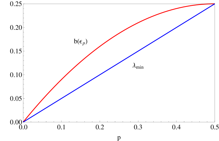
Figure 4: (Color online) The strict difference between the boundariness $b$ (upper line) and minimal eigenvalue $\lambda_{\min}$ (lower line) for erasure channels is illustrated. Let us stress that the difference is not negligible and it is maximal for value $p=1/4$.

The example of a qubit “erasure” channel ${\cal E}_{p}$ illustrates (see Figure 4) that, unlike for states and observables, the boundariness of a channel ${\cal E}$ may differ from the lower bound (10) given by the minimal eigenvalue of the Choi operator $E$. This finding is summarized in the following proposition.

Proposition 5

For qubit “erasure” channels ${\cal E}_{p}$ with $0<p<1/2$ the boundariness is strictly larger than the minimal eigenvalue of the Choi-Jamiolkowski operator. In particular, $b({\cal E}_{p})=p(1-p)>\lambda_{\min}=p/2$.

Further, we will investigate for which channels (if for any) the lower bound on boundariness is tight, i.e. when $b({\cal E}_{p})=\lambda_{min}$. A trivial example is provided by channels from the boundary for which $b({\cal E}_{p})=\lambda_{min}=0$, but are there any other examples? Consider a channel ${\cal E}$ such that the minimal eigenvalue subspace of the associated Choi-Jamiolkowski operator $E$ contains a maximally entangled state. Then a decomposition with $t=\lambda_{min}$ exists and it corresponds to a mixture of a unitary channel (extremal element) and some other channel from the boundary. On the other hand, if the subspace of the minimal eigenvalue of $E$ does not contain any maximally entangled state it is natural to conjecture that the boundariness will be strictly greater then $\lambda_{min}$. The following proposition proves that this conjecture is valid.

Proposition 6

Consider an inner element ${\cal E}$ of the set of channels such that the minimal eigenvalue subspace of its Choi-Jamiolkowski operator $E$ does not contain any maximally entangled state. Then its boundariness is strictly larger than the minimal eigenvalue, i.e. $b(\mathcal{E})>\lambda_{min}$.

Proof. We split the proof into two parts. First, we prove $t_{{\cal E}}(\mathcal{F})>\lambda_{min}$ for any unitary channel $\mathcal{F}$ and then we prove it for any other channel $\mathcal{F}$. Let us write the spectral decomposition of operator $E$ as

$$E =\sum_{k=1}^{r}\lambda_{k}P_{k},$$ (12)

where the eigenvalues $\lambda_{k}>0$ are non-decreasing with $k$ (i.e. $\lambda_{1}=\lambda_{min}$), $P_{k}$ are the projectors onto eigensubspaces corresponding to $\lambda_{k}$ and $\sum_{k}P_{k}=I$ is the identity operator on $\mathcal{H}_{d}\otimes\mathcal{H}_{d}$. Since ${\cal E}$ is an inner point $\lambda_{1}\neq 0$. The Choi-Jamiolkowski operators associated with unitary channels $\mathcal{F}$ have the form $F=|\varphi\rangle\langle\varphi|$, where $|\varphi\rangle$ is a maximally entangled state. The assumption of the proposition implies that $P_{1}|\varphi\rangle\neq|\varphi\rangle$. In order to prove that $t_{{\cal E}}(\mathcal{F})>\lambda_{min}$ it suffices to show that there exists $t>\lambda_{min}$ such that $E-tF\geq 0$ (implying $G=(E-tF)/(1-t)$ describes a quantum channel $\mathcal{G}$). It is useful to write

$$|\varphi\rangle=\sqrt{\alpha}|v\rangle+\sqrt{1-\alpha}|v_{\perp}\rangle,$$ (13)

where $0\leq\alpha<1$, $P_{1}|v\rangle=|v\rangle$ and $P_{1}|v_{\perp}\rangle=0$. Define a positive operator $X=\lambda_{1}|v\rangle\langle v|+\lambda_{2}|v_{\perp}\rangle\langle v_{\perp}|$ and write $E-tF=E-X+X-tF$. The operator $E-X$ is clearly positive. Further, we will show that $X-tF$ is positive when we set $t=\lambda_{1}\lambda_{2}/[\lambda_{1}+(\lambda_{2}-\lambda_{1})\alpha]>\lambda_{\min}$ and as a consequence $E-tF\geq 0$. By definition, $X-tF$ acts nontrivially in two-dimensional subspace spanned by vectors $|v\rangle$ and $|v_{\perp}\rangle$. Within this subspace it has eigenvalues $0$ and $\lambda_{2}+\lambda_{1}-t>0$, hence, it is positive. This concludes the first part of the proof concerning decompositions with unitary channels.

Now, let us assume that the channel $\mathcal{F}$ is not unitary. Since the Choi-Jamiolkowski operator $F$ associated with the channel $\mathcal{F}$ is a density operator, it follows that its maximal eigenvalue $\mu_{max}\leq 1$ (saturated only for unitary channels). Set $t=\lambda_{min}/\mu_{max}$. Then for non-unitary channels $t>\lambda_{\min}$ and since $0<\lambda_{min}\leq 1/d^{2}\leq\mu_{max}$ it follows that $0<t\leq 1$. For all vectors $|\varphi\rangle$

$$\langle\varphi|E-tF|\varphi\rangle\geq\lambda_{min}-\frac{\lambda_{min}}{\mu_{max}}\mu_{max}=0,$$ (14)

and, therefore, $G=(E-tF)/(1-t)\geq 0$, too. As in the first part of the proof this means that $t_{\mathcal{E}}(\mathcal{F})>\lambda_{min}$ for all non-unitary boundary channels $\mathcal{F}$, because we found decomposition $\mathcal{E}=t\mathcal{F}+(1-t)\mathcal{G}$ with $t>\lambda_{min}$.

The above two parts of the proof show that $t_{\mathcal{E}}(\mathcal{F})>\lambda_{min}$ for the channel $\mathcal{E}$ of the claim and for any channel $\mathcal{F}$. The claim follows from the observation that, according to Proposition 1, $b(\mathcal{E})=t_{\mathcal{E}}(\mathcal{F})$ for some (extreme) channel $\mathcal{F}$ and, especially for this optimal channel, $t_{\mathcal{E}}(\mathcal{F})>\lambda_{min}$. $\,\blacksquare$

IV Relation to minimum-error discrimination

Quantum theory is known to be probabilistic, hence, individual outcomes of experiments have typically very limited (if any) operational interpretation. One example of this type is the question of discrimination among a limited number of quantum devices. In its simplest form the setting is the following. We are given an unknown quantum device, which is with equal prior probability either $A$, or $B$ ($A$ and $B$ are known to us). Our task is to design an experiment in which we are allowed to use the given device only once and we are asked to conclude the identity of the device. Clearly, this cannot be done in all cases unless some imperfections are allowed. There are various ways how to formulate the discrimination task.

The most traditional Helstrom ; Holevo one is aimed to minimize the average probability of error of our conclusions. Surprisingly, the success is quantified by norm-induced distances chiribella2009 , hence, the discrimination problem provides a clear operational interpretation of these norms. We may express the optimal error probability of minimum-error discrimination as follows

$$p_{\rm error}(A,B)=\frac{1}{2}(1-\frac{1}{2}\|A-B\|)\,,$$ (15)

where the type of the norm $\|A-B\|$ depends on the considered problem.

Recently, it was shown in Ref. jencova2013 that in general convex settings the so-called base norms are solutions to minimum-error discrimination problems. In particular, it was also shown that base norms coincide with the completely bounded (CB) norms in the case of quantum channels, states and observables, thus, according to Proposition 2 and Eq. (3) the following inequality holds

$$\|A-B\|_{Z}\equiv\|A-B\|_{\rm cb}\leq 2(1-b(A))\,.$$

In rest of this section we will illustrate that for quantum structures the base norms (being completely bounded norms) and boundariness are intimately related. We will investigate how tight the above inequalities are for particular quantum convex sets.

IV.1 States

Let us start with the case of quantum states, for which the CB norm coincides with the trace-norm (see for instance jencova2013 ; chiribella2009 ), i.e. $||A||_{\rm tr}=\mathrm{tr}[|A|]$. Recall that the conclusion of Proposition 2, when applied for states, is

$$\|\varrho-\xi\|_{\rm tr}\leq 2[1-b(\varrho)]\,.$$ (16)

Using the absolute scalability of the norm the roles of $\varrho$ and $\xi$ can be exchanged and from (15) and (16) it follows that

$$p_{\rm error}(\varrho,\xi)\geq\frac{1}{2}\max\{b(\varrho),b(\xi)\}\,,$$

i.e. the mixedness of states measured by their boundariness lower bounds the optimal error probability of discrimination between them. Moreover, for a given state $\varrho$ we may write

$$\min_{\xi}p_{\rm error}(\varrho,\xi)\geq\frac{1}{2}b(\varrho)\,,$$

hence interpreting the boundariness as the limiting value of the best distinguishability of the state $\varrho$ from any other state. In other words, the boundariness determines the information potential of the state as the distinguishability of states is the key figure of merit for quantum communication protocols wilde2013 .

As before, let $|\psi\rangle$ be the state for which $\varrho|\psi\rangle=\lambda_{\min}|\psi\rangle$. It is straightforward to see that

$$\|\varrho-|\psi\rangle\langle\psi|\|_{\rm tr}=2(1-\lambda_{\min})\,.$$

Hence, the upper bound (16) can be saturated and we have proven the following proposition.

Proposition 7

For a given state $\varrho$

$$\sup_{\xi}\|\varrho-\xi\|_{\rm tr}=2(1-b(\varrho))\,.$$

In particular, this implies that the states from the boundary (with $b(\varrho)=0$) can be used as noiseless carriers of bits of information as for each of them one can find a perfectly distinguishable ”partner” state.

IV.2 Observables

For observables we may formulate an analoguous result:

Proposition 8

Suppose that $\mathsf{C}$ is an $n$-valued observable. Then

$$\sup_{\mathsf{A}}\|\mathsf{C}-\mathsf{A}\|=2(1-b(\mathsf{C}))\,,$$

where $\|\cdot\|$ is the base norm (identified with completely bounded norm) for observables.

Proof. We will prove that $\mathsf{A}$ defined in Eq. (9) yields the supremum of the claim. Let us recall that $|\psi\rangle$ (used in definition of $\mathsf{A}$) is the vector defined by the relation $C_{k}|\psi\rangle=\lambda_{\min}|\psi\rangle$ for some $k$. According to Proposition 2

$$\|\mathsf{C}-\mathsf{A}\|\leq 2(1-\lambda_{\min})\,,$$ (17)

where the norm $\|\mathsf{C}-\mathsf{A}\|$ (the base norm $=$ completely bounded norm $=$ diamond norm) can be evaluated as jencova2013

$$\|\mathsf{C}-\mathsf{A}\| = \sup_{\varrho}\sum_{j}|\mathrm{tr}[\varrho(C_{j}-A_{j})]|$$

Assuming $\varrho=|\psi\rangle\langle\psi|$ we obtain

$$\|\mathsf{C}-\mathsf{A}\|\geq 1-\lambda_{\min}+\sum_{j\neq k}\langle\psi|C_{j}|\psi\rangle$$

because $\langle\psi|A_{j}|\psi\rangle=0$ for $j\neq k$, $\langle\psi|A_{k}|\psi\rangle=1$ and $\langle\psi|C_{k}|\psi\rangle=\lambda_{\min}$. Moreover, since $\sum_{j\neq k}\langle\psi|C_{j}|\psi\rangle=1-\langle\psi|C_{k}|\psi\rangle=1-\lambda_{\min}$ we find that for the chosen observables $\mathsf{C}$, $\mathsf{A}$ we have $\|\mathsf{C}-\mathsf{A}\|\geq 2(1-\lambda_{\min})$. Combining this with the lower bound (17) valid for any observable we have proven the proposition. $\,\blacksquare$

IV.3 Channels

For channels the boundariness is not given by minimal eigenvalue of the Choi-Jamiolkowski operator. Actually, we are missing an analytical form of channel’s boundariness. Hence, in general the saturation of the inequality

$$\sup_{\mathcal{F}}\|\mathcal{E}-\mathcal{F}\|_{\rm cb}\leq 2(1-b(\mathcal{E}))$$ (18)

is open and we chose to test the saturation of the bound for the examples of quantum channels that we studied in Section III.3. Let us stress that analytical expressions of the completely bounded norm are rather rare, but there exist efficient numerical methods for its evaluation watrous2009 .

For the qubit “erasure” channel ${\cal E}_{p}$ that transforms an arbitrary input state $\varrho$ into a fixed output state $\xi_{p}=p|0\rangle\langle 0|+(1-p)|1\rangle\langle 1|$ the completely bounded norm $\|{\cal E}_{p}-\mathcal{F}\|_{\rm cb}$ can be expressed as

$$\|{\cal E}_{p}-\mathcal{F}\|_{\rm cb}=\sup_{\|\psi\|=1}\|({\cal E}_{p}-\mathcal{F})\otimes\mathcal{I}(|\psi\rangle\langle\psi|)\|_{\rm tr},$$ (19)

where $\mathcal{I}$ is the qubit identity channel and $|\psi\rangle$ is a two qubit state. Choice of $\mathcal{F}=\mathcal{I}$ and

$$|\psi\rangle=\sqrt{1-p}|0\rangle\otimes|0\rangle+\sqrt{p}|1\rangle\otimes|1\rangle$$ (20)

lower bounds the norm in (18) by $2(1-p(1-p))$ as can be seen by direct calculation. Due to the result $b({\cal E}_{p})=p(1-p)$ from section III.3 this can be equivalently written as $2(1-b({\cal E}_{p}))\leq\sup_{\mathcal{F}}\|{\cal E}_{p}-\mathcal{F}\|_{\rm cb}$, which implies that the bound (18) is tight for the channel ${\cal E}_{p}$.

Let us, further, consider the class of channels whose Choi operator $E$ contains some maximally entangled state $|\phi\rangle$ in its minimal eigenvalue subspace. For these channels $b({\cal E})=\lambda_{min}$ (see section III.3). Choose $\mathcal{F}$ to be a unitary channel, i.e. $F=|\phi\rangle\langle\phi|$ and set $|\psi\rangle=1/\sqrt{2}(|0\rangle\otimes|0\rangle+|1\rangle\otimes|1\rangle)$ (maximally entangled state). Then

$$\|E-F\|_{\rm tr}=\|({\cal E}-\mathcal{F})\otimes\mathcal{I}(|\psi\rangle\langle\psi|)\|_{\rm tr}\leq\|{\cal E}-\mathcal{F}\|_{\rm cb},$$

and direct calculation gives $\|E-F\|_{\rm tr}=2(1-\lambda_{min})=2(1-b({\cal E}))$. Altogether, we have shown

$$2(1-b({\cal E}))\leq\sup_{\mathcal{F}}\|{\cal E}-\mathcal{F}\|_{\rm cb},$$ (21)

which means that for this type of channels the bound (18) is tight.

V Summary

Convexity is one of the main mathematical features of modern science and it is natural to ask how the physical concepts and structures are interlinked with the existing convex structure. Using only the convexity we introduced the concept of boundariness and investigated its physical meaning in statistical theories such as quantum mechanics. Intuitively, the boundariness quantifies how far an element of the convex set is from its boundary. The definition of the boundary is based solely on the convexity and no other mathematical structure of the set is assumed.

We have shown that the value of boundariness $b(y)$ identifies the most non-uniform convex decomposition of inner element $y$ into a pair of boundary elements. Further, we showed (Proposition 1) that for compact convex sets such optimal decomposition is achieved when one of the boundary points is also extremal. This surprising property simplifies significantly our analysis of quantum convex sets and allowes us to evaluate the value of boundariness.

In particular, we have found that, in contrast to the case of states and observables, for channels the general lower bound on boundariness ($b\geq\lambda_{\min}$) given by the minimal eigenvalue of the Choi-Jamiolkowski representation is not saturated (see Section III). We illustrated this feature explicitely for the class of qubit “erasure” channels ${\cal E}_{p}$ mapping whole state space into a fixed state $\xi_{p}=p|0\rangle\langle 0|+(1-p)|1\rangle\langle 1|$ ($0<p<1/2$). The boundariness of this channel was found to be $b({\cal E}_{p})=p(1-p)>\lambda_{\min}=p/2$ (Proposition 5). We showed that the saturation of the bound is equivalent with existence of maximally entangled state in the minimal eigenvalue subspace of the channel’s Choi-Jamiolkowski operator. Let us stress that the boundariness vanishes for infinite dimensional systems, because the associated convex sets contain no interior points (discussed in Appendix B).

Concerning the operational meaning of boundariness, we first demonstrated that the boundariness can be used to upper bound any (semi)norm induced distance providing the (semi)norm is bounded on the convex set. An example of such norm is the base norm which is induced solely by the convex structure of the set. Recently, it was shown in Ref. jencova2013 that for the sets of quantum states, measurements and evolutions base norms coincide with so-called completely bounded norms. These norms are known chiribella2009 ; gutoski2012 to appear naturally in quantum minimum error discrimination tasks. As a result, this connection provides a clear operational interpretation for the boundariness as described in Section IV.

More precisely, if we want to determine in which of the two known (equally likely) possibilities $A$ or $B$ an unknown state (or measurement, or channel) was prepared and given to us, the probability of making an erroneous conclusion exceeds one half times the boundariness for any of the elements $A$ and $B$. For a generic pair of possibilities $A$ and $B$ this bound is not necessarily tight, however if we keep $A$ fixed then the boundariness of $A$ is proportional to the minimum error probability discrimination of $A$ and the most distinguishable quantum device from $A$. To be precise this was shown only for states and observables (in which case the analytic formula for boundariness was derived), but we conjecture that this feature holds also for quantum channels. We verified this conjecture for erasure channels and the class of channels containing a maximally entangled state in the minimum eigenvalue subspace of their Choi-Jamiolkoski operators.

In conclusion let us mention a rather intriguing observation. In all the cases we have met the “optimal” decompositions (determining the value of boundariness) contain pure states, sharp observables and unitary channels. In other words, only special subsets of extremal elements (for observables and channels) are needed. This is true for all states and for all observables. The case of channels is open, but no counter-example is known. This observation suggests that the concept of boundariness could provide some operational meaning to sharpness of observables and unitarity of evolution.

Appendix A Properties of the weight function

The purpose of this appendix is to prove results that are needed for Proposition 1. Let us first recall a few basic definitions in linear analysis. Suppose that $V$ is a real vector space. For a subset $X\subset V$ we denote by $V_{X}$ the smallest affine subspace of $V$ containing $X$. For any $x\in X$, the linear subspace $V_{X}-x$ is just the linear hull of $X-x$, where we introduced the notation $X-x\equiv\{y-x\,|\,y\in X\}$. We say that $U\subset V$ is absorbing if for every $v\in V$ there is $\alpha>0$ such that $\alpha^{-1}v\in U$; especially $0\in U$. The following lemma gives another characterization for the boundary of a convex set $Z$, which is useful for studying the continuity properties of the weight function.

Lemma 2

Suppose that $Z$ is a convex subset of a real vector space $V$. An element $y\in Z$ is inner, i.e., $y\in Z\setminus\partial Z$ if and only if $Z-y$ is absorbing in the subspace $V_{Z}-y$.

Proof. Let us assume that $y$ is an inner point of $Z$ and suppose that $v\in V_{Z}-y$. For simplicity, let us assume that $v\neq 0$. The convexity of $Z-y$ and the definition of $V_{Z}$ yield that there are $d_{+},\,d_{-}\in Z-y$ and $\lambda_{+},\,\lambda_{-}\geq 0$, where $\lambda_{+}>0$ or $\lambda_{-}>0$ such that $v=\lambda_{+}d_{+}-\lambda_{-}d_{-}$. The fact that $y$ is an inner point implies that when $d_{-}\in Z-y$ then $\exists q>0$ such that $-qd_{-}\in Z-y$. Hence, $v=\alpha d$, where $\alpha=\lambda_{+}+\lambda_{-}/q>0$, $d=\frac{\lambda_{+}}{\alpha}d_{+}+\frac{\lambda_{-}}{q\alpha}(-qd_{-})\in Z-y$, which proves that $Z-y$ is absorbing in $V_{Z}-y$. Suppose now that $Z-y$ is absorbing in $V_{Z}-y$ and $x\in Z$, so that $x-y=d\in Z-y$. Also $-d\in V_{Z}-y$ and because $Z-y$ is absorbing, there is $\alpha>0$ such that $-\alpha^{-1}d\in Z-y$, i.e., $y-\alpha^{-1}d=z\in Z$ and

$$y=\frac{1}{1+\alpha}x+\frac{\alpha}{1+\alpha}z.$$

This means that for all $x\in Z$, $x\leq_{C}y$, i.e., $y\notin\partial Z$. $\,\blacksquare$

The weight function can be associated with a function called as Minkowski gauge. This connection gives more insight in the properties of the weight function in the infinite-dimensional case. When $A$ is an absorbing subset of a real vector space $W$, we may define a function $P_{A}:W\to\mathbb{R}$,

$$P_{A}(w)=\inf\{\alpha\geq 0\,|\,\alpha^{-1}w\in A\},\quad w\in W.$$

$P_{A}$ is called the Minkowski gauge of $A$. For basic properties of this function, we refer to infdimanalysis . If $A$ is convex, then $P_{A}$ is a convex function, and

$$\{v\in W\,|\,P_{A}(v)<1\}\subset A\subset\{v\in W\,|\,P_{A}(v)\leq 1\}.$$

When $A$ is an absorbing convex balanced subset, $P_{A}$ has many properties reminiscent to a norm, whose unit ball is $A$. When $W$ is a (locally convex) topological vector space, the Minkowski gauge $P_{A}$ is continuous if and only if $A$ is a neighbourhood of the origin.

Suppose that $Z$ is a convex subset of a real vector space $V$ and $y\in Z$. The basis for connecting a Minkowski gauge to the weight function $t_{y}$ is provided by the following observation: Consider a vector $y-x\in V_{Z}-y$, where $x\in Z$. As can be seen from Fig. (5), the scaling factor $\alpha$ that shrinks or extends this vector to the border of the set $Z-y$ defines a point $z(t)$, which determines the value of the weight function $t_{y}$. These considerations can be formulated mathematically as follows: Pick $t\in[0,t_{y}(x))$ and define $z(t)=(1-t)^{-1}(y-tx)\in Z$. Now $z(t)-y=t(1-t)^{-1}(y-x)\in Z-y$. As $t$ approaches $t_{y}(x)$ from below, $\alpha(t)=(1-t)/t$ decreases and from this we see that $\big{(}1-t_{y}(x)\big{)}/t_{y}(x)=P_{Z-y}(y-x)$ or, when we denote the Minkowski gauge $P_{Z-y}:V_{Z}-y\to[0,\infty)$ of $Z-y$ by $p_{y}(x)\equiv P_{Z-y}(y-x)$,

$$t_{y}(x)=\frac{1}{1+p_{y}(x)}.$$ (22)

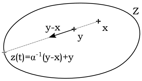
Figure 5: The scalar $\alpha$ extending $y-x$ from the starting point $y$ to the boundary coincides with the Minkowski gauge $P_{Z-y}(y-x)$ and the decomposition of $y$ with respect to this boundary point and $x$ gives the value $t_{y}(x)$ of the weight function.

According to Lemma 2 the gauge $p_{y}$ is well defined, when $y\in Z\setminus\partial Z$. From the convexity of the Minkowski gauge we again see that $x\mapsto 1/t_{y}(x)=1+p_{y}(x)$ is convex on $Z$ whenever $y\in Z\setminus\partial Z$. We immediately see that, in the case of a topological vector space $V$, whenever $y\in Z\setminus\partial Z$, the weight function $t_{y}$ is continuous if and only if the Minkowski gauge $p_{y}$ is continuous, i.e., $Z-y$ is a neighbourhood of the origin of $V_{Z}-y$. In finite-dimensional settings, any convex absorbing set is a neighbourhood of origin (as one may easily check). Thus we obtain the following result needed for proving Proposition 1.

Proposition 9

Suppose that $Z\subset\mathbb{R}^{n}$ for some $n\in\mathbb{N}$. The weight function $t_{y}$ is continuous if and only if $y\in Z\setminus\partial Z$.

The quantum physical sets of states, POVMs and channels are all compact (even in the infinite-dimensional case with respect to suitable topologies), implying that, e.g., Proposition 1 is applicable for the sets of (finite dimensional) quantum devices.

Appendix B Relation to Hilbert’s projective metric

The weight function is also related to the Hilbert’s projective metric. Suppose $C\subset V$ is a pointed generating cone of a real vector space $V$ (see definition in Section II). We may define the functions

$$\inf(v/w) = \sup\{\lambda\in\mathbb{R}\,|\,v-\lambda w\in C\},$$

$$\sup(v/w) = \inf\{\lambda\in\mathbb{R}\,|\,\lambda w-v\in C\},$$

$v,\,w\in V$. Through these functions, one can define Hilbert’s projective metric $\mathfrak{h}:V\times V\to[0,\infty]$, $\mathfrak{h}(v,w)=\ln{\big{(}\sup(v/w)/\inf(v/w)\big{)}}$ that can be lifted into a well-defined metric in the projective space $\mathbb{P}V$; for more on this subject, see eveson1990 ; reeb_etal2011 ; gaubert2013

When $Z$ is a base for $C$, one can easily show that, for $x,\,y\in Z$, $\inf(y/x)=\sup\{t\in[0,1)\,|\,y-tx\in C\}$. Moreover, if $x,\,y\in Z$ and $y-tx\in C$ for some $t\in[0,1)$, then $y-tx=sz$ for some (unique) $s\geq 0$ and $z\in Z$. If $s\neq 1-t$, then one sees that both $y\in Z$ and

$$\frac{1}{s+t}\;y=\frac{t}{s+t}\;x+\frac{s}{s+t}\;z$$ (23)

belongs to $Z$ contradicting the fact that $Z$ is a base. Hence $s=1-t$ and

$$\inf(y/x)=\sup\{t\in[0,1)\,|\,y-tx\in(1-t)Z\}=t_{y}(x).$$

Similarly, the convex function $x\mapsto 1/t_{y}(x)$ is associated with the $\sup$-function.

Appendix C Boundary of quantum convex sets

The question of the boundary elements for states, observables and channels can be treated in a unified way as all these objects can be understood as transformations represented by completely positive linear maps. In this section, we give conditions of being on the boundary for all relevant quantum devices. For the sake of brevity, we characterize the boundary for all relevant quantum convex sets in one go. This, however, necessitates the use of Heisenberg picture which is used only in this section.

Let us fix a Hilbert space $\mathcal{H}$ and a unital $C^{*}$-algebra $\mathcal{A}$. We say that a linear map $\Phi:\mathcal{A}\to\mathcal{L}(\mathcal{H})$ is completely positive (CP) if for any $n=1,\,2,\ldots$ and $a_{1},\ldots,\,a_{n}\in\mathcal{A}$ and $|v_{1}\rangle,\ldots,\,|v_{n}\rangle\in\mathcal{H}$

$$\sum_{j,k=1}^{n}\langle v_{j}|\Phi(a_{j}^{\dagger}a_{k})|v_{k}\rangle\geq 0.$$

For any CP map $\Phi$ there is a Hilbert space $\mathcal{M}$, a linear map $J:\mathcal{H}\to\mathcal{M}$ and a linear map $\pi:\mathcal{A}\to\mathcal{L}(\mathcal{M})$ such that $\pi(1)=I_{\mathcal{M}}$, $\pi(a^{\dagger})=\pi(a)^{\dagger}$ and $\pi(ab)=\pi(a)\pi(b)$ for all $a,\,b\in\mathcal{A}$ (i.e., $\pi$ is a unital *-representation of $\mathcal{A}$ on $\mathcal{M}$) that constitute a minimal Stinespring dilation for $\Phi$. This means that $\Phi(a)=J^{\dagger}\pi(a)J$ for all $a\in\mathcal{A}$ and the subspace of $\mathcal{M}$ generated by the vectors $\pi(a)J|v\rangle$, $a\in\mathcal{A}$, $|v\rangle\in\mathcal{H}$, is dense in $\mathcal{M}$.

In what follows, we only study unital CP maps, i.e., $\Phi(1_{\mathcal{A}})=I_{\mathcal{H}}$. We denote the set of all unital CP maps $\Phi:\mathcal{A}\to\mathcal{L}(\mathcal{H})$ by $\mathcal{CP}(\mathcal{A};\mathcal{H})$. Since the set $\mathcal{CP}(\mathcal{A};\mathcal{H})$ is convex, it is equipped with the preorder $\leq_{C}$. We denote $\Phi=_{C}\Psi$ if $\Phi\leq_{C}\Psi$ and $\Psi\leq_{C}\Phi$. For any $\Psi\in\mathcal{CP}(\mathcal{A};\mathcal{H})$ we may define the set

$$\mathcal{F}(\Psi)=\{\Phi\in\mathcal{CP}(\mathcal{A};\mathcal{H})\,|\,\Phi\leq_{C}\Psi\}.$$

Let us fix a minimal dilation $(\mathcal{M},\pi,J)$ for $\Psi$. Let us define $F(\Psi)$ as the set of positive operators $E\in\mathcal{L}(\mathcal{M})$ such that $E\pi(a)=\pi(a)E$ for all $a\in\mathcal{A}$ and $J^{\dagger}EJ=I$. The following proposition is essentially due to raginsky2003 .

Proposition 10

Suppose that $\Psi\in\mathcal{CP}(\mathcal{A};\mathcal{H})$ is equipped with the minimal dilation $(\mathcal{M},\pi,J)$. The sets $\mathcal{F}(\Psi)$ and $F(\Psi)$ are in one-to-one correspondence set up by

$$\Phi(a)=J^{\dagger}\pi(a)EJ,\qquad\Phi\in\mathcal{F}(\Psi),\quad E\in F(\Psi)$$ (24)

for all $a\in\mathcal{A}$.

Lemma 3

Suppose that $\Phi,\,\Psi\in\mathcal{CP}(\mathcal{A};\mathcal{H})$ and fix the minimal dilation $(\mathcal{M},\pi,J)$ for $\Psi$. Now $\Phi=_{C}\Psi$ if and only if there is $E\in F(\Psi)$ with bounded inverse such that $\Phi(a)=J^{\dagger}\pi(a)EJ$ for all $a\in\mathcal{A}$.

Proof. Case $\Phi=\Psi$ is obvious. Let us concentrate on the case $\Phi\neq\Psi$.

Let us assume that $\Phi=_{C}\Psi$. Because, especially, $\Phi\leq_{C}\Psi$, there is an operator $E\in F(\Psi)$ such that $\Phi(a)=J^{\dagger}\pi(a)EJ$ for all $a\in\mathcal{A}$. Denote the closure of the range of $\sqrt{E}$ by $\mathcal{M}_{E}$ and the projection of $\mathcal{M}$ onto this subspace by $P_{E}$. Since $E$ commutes with $\pi$, also $P_{E}$ commutes with $\pi$, and we may define the map $\pi_{E}:\mathcal{A}\to\mathcal{L}(\mathcal{M}_{E})$, $\pi_{E}(a)=P_{E}\pi(a)|_{\mathcal{M}_{E}}$. Also define $J_{E}=\sqrt{E}J$. It is straight-forward to check that the triple $(\mathcal{M}_{E},\pi_{E},J_{E})$ constitutes a minimal dilation of $\Phi$. Since also $\Psi\leq_{C}\Phi$ and $\Phi\neq\Psi$, it follows that there is $t\in(0,1)$ and $\Psi^{\prime}\in\mathcal{CP}(\mathcal{A};\mathcal{H})$ such that $\Phi=t\Psi+(1-t)\Psi^{\prime}$. In other words, there is a number $t\in(0,1)$ such that the map $\Psi^{\prime}$,

$$\Psi^{\prime}(a)=\frac{1}{1-t}(\Phi-t\Psi)=\frac{1}{1-t}J^{\dagger}\pi(a)(E-tI)J,\qquad a\in\mathcal{A},$$

is completely positive or, equivalently, $E\geq tI$. Hence $E$ has a bounded inverse.

Suppose that $E\in F(\Psi)$ is as in the first part of the proof and $E^{-1}\in\mathcal{L}(\mathcal{M})$. From Proposition 10 it follows immediately that $\Phi\leq_{C}\Psi$. Denote $E^{\prime}=P_{E}E^{-1}|_{\mathcal{M}_{E}}$. We have $E^{\prime}\geq 0$, $J_{E}^{\dagger}E^{\prime}J_{E}=J^{\dagger}J=I$ and

$$E^{\prime}\pi_{E}(a) = P_{E}E^{-1}\pi(a)|_{\mathcal{M}_{E}}=P_{E}E^{-1}\pi(a)EE^{-1}|_{\mathcal{M}_{E}}$$

$$= P_{E}E^{-1}E\pi(a)E^{-1}|_{\mathcal{M}_{E}}=P_{E}\pi(a)E^{-1}|_{\mathcal{M}_{E}}$$

$$= \pi_{E}(a)E^{\prime}$$

for all $a\in\mathcal{A}$, so that $E^{\prime}\in F(\Phi)$ when we fix the dilation $(\mathcal{M}_{E},\pi_{E},J_{E})$ for $\Phi$. Furthermore

$$J_{E}^{\dagger}\pi_{E}(a)E^{\prime}J_{E}=J^{\dagger}\pi(a)\sqrt{E}E^{-1}\sqrt{E}J=J^{\dagger}\pi(a)J=\Psi(a)$$

for all $a\in\mathcal{A}$. According to Proposition 10 this means that $\Psi\leq_{C}\Phi$. $\,\blacksquare$

We denote the spectrum of an operator $E\in\mathcal{L}(\mathcal{M})$ on a Hilbert space $\mathcal{M}$ by $\mathrm{sp}(E)$. The following proposition, which is an immediate corollary of the previous lemma, characterizes the boundary elements of the set of unital CP maps.

Proposition 11

Suppose that $\Phi\in\mathcal{CP}(\mathcal{A};\mathcal{H})$. The map $\Phi$ is on the boundary of $\mathcal{CP}(\mathcal{A};\mathcal{H})$ if and only if there is $\Psi\in\mathcal{CP}(\mathcal{A};\mathcal{H})$ with a minimal dilation $(\mathcal{M},\pi,J)$ such that $\Phi\leq_{C}\Psi$ and $\Phi$ corresponds to an operator $E\in F(\Psi)$ with $0\in\mathrm{sp}(E)$.

Proof. The condition $\Phi\in\partial\mathcal{CP}(\mathcal{A};\mathcal{H})$ is equivalent with the fact that there is $\Psi\in\mathcal{CP}(\mathcal{A};\mathcal{H})$ such that $\Phi\leq_{C}\Psi$ but $\Psi\not\leq_{C}\Phi$. Indeed, if $\Psi^{\prime}\in\mathcal{CP}(\mathcal{A};\mathcal{H})$ is such that $\Psi^{\prime}\not\leq_{C}\Phi$, we may define $\Psi=\frac{1}{2}\Phi+\frac{1}{2}\Psi^{\prime}$ so that $\Phi\leq_{C}\Psi$. Moreover, if $\Psi\leq_{C}\Phi$, it would follow that $\Psi^{\prime}\leq_{C}\Psi\leq_{C}\Phi$ yielding $\Psi^{\prime}\leq\Phi$ yielding a contradiction. Suppose that $\Psi\in\mathcal{CP}(\mathcal{A};\mathcal{H})$ is such that $\Phi\leq_{C}\Psi$ and $\Psi\not\leq_{C}\Phi$ and $\Psi$ has the minimal dilation $(\mathcal{M},\pi,J)$ and $\Phi$ corresponds to the operator $E\in F(\Psi)$ according to Equation (24). According to Lemma 3, the condition $\Psi\not\leq_{C}\Phi$ is equivalent to $E$ not having a bounded inverse or, in other words, $0\in\mathrm{sp}(E)$. $\,\blacksquare$

The CP maps of quantum physics are normal. This is because in this section we have described our quantum devices jointly in Heisenberg picture and, in order to transcend to the Schrödinger picture, we generally need normality. However, when $\mathcal{H}$ and $\mathcal{A}$ are finite dimensional the maps $\Phi\in\mathcal{CP}(\mathcal{A};\mathcal{H})$ are automatically normal. The results of this section also hold for the restricted class of normal elements in $\mathcal{CP}(\mathcal{A};\mathcal{H})$ because this class is a face of $\mathcal{CP}(\mathcal{A};\mathcal{H})$, i.e., if $\Phi$ is normal and $\Phi^{\prime}\leq_{C}\Phi$ then also $\Phi^{\prime}$ is normal.

C.1 States

Suppose that $\mathcal{K}$ is a Hilbert space. We will denote the set of states by $\mathcal{S}(\mathcal{K})$ containing positive trace-class operators on $\mathcal{K}$ with trace 1. The states are in one-to-one correspondence with the normal (completely) positive unital maps $\varphi:\mathcal{L}(\mathcal{K})\to\mathbb{C}$, i.e. the set of normal elements in $\mathcal{CP}\big{(}\mathcal{L}(\mathcal{K});\mathbb{C}\big{)}$.

Proposition 12

A state $\varrho\in\partial\mathcal{S}(\mathcal{K})$ if and only if $\rho$ has 0 in its spectrum.

Proof. First, let us assume that $\dim{\mathcal{K}}<\infty$. Suppose that $\varrho\in\mathcal{S}(\mathcal{K})$ is such that there is a unit vector $|v\rangle\in\mathcal{K}$ such that $\varrho|v\rangle=0$. Let us define the operator $D=|v\rangle\langle v|-(d-1)^{-1}(I-|v\rangle\langle v|)$. Denote the smallest non-zero eigenvalue of $\varrho$ by $\lambda_{min}$. It is easy to see that whenever $\varepsilon\leq\lambda_{\min}$, $\varrho+\varepsilon D\in\mathcal{S}(\mathcal{K})$ but $\varrho-\varepsilon D$ is not positive for any $\varepsilon>0$. Hence $\varrho\in\partial\mathcal{S}(\mathcal{K})$.

Suppose now $\varrho\in\partial\mathcal{S}(\mathcal{K})$, i.e., there is a state $\sigma\in\mathcal{S}(\mathcal{K})$ such that when we denote $D=\sigma-\varrho$, then $\varrho-\varepsilon D$ is not positive for any $\varepsilon>0$. We may write $\mathcal{K}=\mathcal{K}_{+}\oplus\mathcal{K}_{0}\oplus\mathcal{K}_{-}$, where $\mathcal{K}_{+}$ is the direct sum of the eigenspaces corresponding to the positive eigenvalues of $D$ and $\mathcal{K}_{0}$ is the kernel of $D$. We infer that $\mathcal{K}_{+}\cap\ker{\varrho}$ is non-trivial and hence also $\ker{\varrho}$ is non-trivial. This means that $0$ is an eigenvalue of $\varrho$.

Now, let us assume that $\mathcal{K}$ is infinite dimensional. Assume that $\varrho\in\mathcal{S}(\mathcal{K})$ would be in the interior, i.e., $\varrho\notin\partial\mathcal{S}(\mathcal{K})$. Then, especially, $|v\rangle\langle v|\leq_{C}\varrho$ for all unit vectors $|v\rangle\in\mathcal{K}$. Whenever $\lambda|v\rangle\langle v|\leq A$ for some $\lambda>0$ and some positive $A\in\mathcal{L}(\mathcal{K})$, it follows buschgudder that $|v\rangle\in\mathrm{ran}(\sqrt{A})$ or, in other words, $|v\rangle=\sqrt{A}|w\rangle$ for some $|w\rangle\in\mathcal{K}$. In the case where $A$ is a state operator, this result was already proven in hadjisavvas . Hence, $\mathrm{ran}(\sqrt{\varrho})=\mathcal{K}$, i.e., $\sqrt{\varrho}$ is surjective. If $\varrho$ had a non-trivial kernel, it could not be in the interior for then $|v\rangle\langle v|\not\leq_{C}\varrho$ for any unit vector $|v\rangle\in\mathrm{ker}(\varrho)$. Hence, $\rho$ is injective and so $\sqrt{\varrho}$ is injective as well. All this implies that $\sqrt{\varrho}:\mathcal{K}\to\mathcal{K}$ is a bijection and the open mapping theorem yields that there is a continuous inverse $\sqrt{\varrho}^{-1}:\mathcal{K}\to\mathcal{K}$. Hence, there is a bounded inverse $\varrho^{-1}=\sqrt{\varrho}^{-1}\sqrt{\varrho}^{-1}$. However, this is impossible, since in the infinite-dimensional case all state operators have 0 in their spectra. $\,\blacksquare$

The previous proposition tells us that the boundary of the set of states depends dramatically on the dimensionality of the Hilbert space: If the space is finite dimensional, boundary states are exactly those whose kernel is non-trivial. In the infinite-dimensional case, the set of states coincides with its boundary.

C.2 Effects and finite outcome observables

Denote $\Omega=\{1,\ldots,\,N\}$ and define $\mathcal{O}^{N}(\mathcal{H})$ as the set of positive-operator-valued measures on $\mathcal{H}$ and taking values in $\Omega$ ($N$-outcome observables), i.e., $\mathsf{M}\in\mathcal{O}^{N}(\mathcal{H})$ is a collection $\mathsf{M}=\{M_{j}\}_{j=1}^{N}$ of positive operators on $\mathcal{H}$ such that $\sum_{j=1}^{N}M_{j}=I$. It should be noted that whenever $\mathsf{M}\in\mathcal{O}^{N}(\mathcal{H})$ then $\mathsf{M}\leq_{C}\mathsf{E}^{N}$, where $\mathsf{E}^{N}=\{E_{j}^{N}\}_{j=1}^{N}$, $E_{j}^{N}=N^{-1}I$ for all $j=1,\ldots,\,N$. Note that we may identify $\mathcal{O}^{N}(\mathcal{H})$ with the set of normal elements in $\mathcal{CP}(\mathcal{A}^{N},\mathcal{H})$, where $\mathcal{A}^{N}$ is just the algebra $\mathbb{C}^{N}$ with componentwise operations.

Proposition 13

The boundary $\partial\mathcal{O}^{N}(\mathcal{H})$ consists of POVMs $\mathsf{M}=\{M_{j}\}$ with $0\in\mathrm{sp}(\mathsf{M}_{j})$ for some $j=1,\ldots,\,N$.

Proof. Endow $\mathbb{C}^{N}$ with an orthonormal basis $\{|1\rangle,\ldots\,|N\rangle\}$ and denote $P_{r}=|r\rangle\langle r|$, $r=1,\ldots\,N$. Define the PVM $\mathsf{Q}\in\mathcal{O}^{N}(\mathcal{H}\otimes\mathbb{C}^{N})$, $Q_{r}=I\otimes P_{r}$, $r=1,\ldots\,N$, and the isometry $J:\mathcal{H}\to\mathcal{H}\otimes\mathbb{C}^{N}$, $J|v\rangle=N^{-1/2}|v\rangle\otimes(|1\rangle+\cdots+|N\rangle)$. It is immediately seen that $(\mathcal{H}\otimes\mathbb{C}^{N},\mathsf{Q},J)$ is a minimal dilation of $\mathsf{E}^{N}=\{N^{-1}I,\ldots\,N^{-1}I\}$, i.e., $J^{\dagger}Q_{r}J=N^{-1}I$, $r=1,\ldots\,2$. Let $F(\mathsf{E}^{N})$ be the set of positive operators $E$ on $\mathcal{H}\otimes\mathbb{C}^{N}$ that commute with $\mathsf{Q}$ and $J^{\dagger}EJ=I$ so that $\mathcal{O}^{N}(\mathcal{H})$ is in one-to-one affine correspondence with $F(\mathsf{E}^{N})$. It follows that $F(\mathsf{E}^{N})$ consists of operators of the form $\sum_{j=1}^{N}A_{j}\otimes P_{j}$, where $A_{j}\in\mathcal{L}(\mathcal{H})$ are positive operators with $A_{j}\leq 2I$. Any $\mathsf{M}\in\mathcal{O}^{N}(\mathcal{H})$ corresponds to such an operator, where $A_{j}=2M_{j}$. A POVM $\mathsf{M}$ is thus on the boundary if and only if the corresponding operator $2\sum_{j=1}^{N}M_{j}\otimes P_{j}$ has 0 in its spectrum. This happens exactly when $0\in\mathrm{sp}(M_{j})$ for some $j$. $\,\blacksquare$

It is often denoted $\mathcal{O}^{2}(\mathcal{H})=\mathcal{E}(\mathcal{H})$ and $\mathsf{E}\in\mathcal{E}(\mathcal{H})$ are called effects. An effect $\mathsf{E}=\{E_{1},E_{2}\}\in\mathcal{E}(\mathcal{H})$ is usually identified with its value $E_{1}$ and hence effects are characterized as positive operators $E\in\mathcal{L}(\mathcal{H})$ with $E\leq I$. One easily sees from the previous proposition that an effect $E$ is on the boundary if and only if $0\in\mathrm{sp}(E)$ or $1\in\mathrm{sp}(E)$.

C.3 Channels

In this subsection, we assume that $\mathcal{H}$ and $\mathcal{K}$ are (separable) Hilbert spaces. We denote by $\mathcal{C}(\mathcal{K};\mathcal{H})$ the set of (normal) unital CP maps $\mathcal{E}:\mathcal{L}(\mathcal{K})\to\mathcal{L}(\mathcal{H})$ and call these maps as channels. Note the the physical input space of these channels is $\mathcal{H}$ and output is $\mathcal{K}$. The minimal Stinespring dilation $(\mathcal{M},\pi,J)$ of a channel $\mathcal{E}\in\mathcal{C}(\mathcal{K};\mathcal{H})$ can be chosen so that $\mathcal{M}$ is separable and $\pi:\mathcal{L}(\mathcal{K})\to\mathcal{L}(\mathcal{H})$ is a normal unital *-representation. This means that there is a separable Hilbert space $\mathcal{K}^{\prime}$ such that we may choose $\mathcal{M}=\mathcal{K}\otimes\mathcal{K}^{\prime}$ and $\pi(B)=B\otimes I_{\mathcal{K}^{\prime}}$ for all $B\in\mathcal{L}(\mathcal{K})$. Hence we usually denote a minimal Stinespring dilation of a channel $\mathcal{E}$ in the form $(\mathcal{K}^{\prime},J)$ where $J:\mathcal{H}\to\mathcal{K}\otimes\mathcal{K}^{\prime}$ is an isometry such that

$$\mathcal{E}(B)=J^{\dagger}(B\otimes I_{\mathcal{K}^{\prime}})J,\qquad B\in\mathcal{L}(\mathcal{K}).$$

Suppose that $\mathcal{K}$ is infinite-dimensional and $\mathcal{E}\in\mathcal{C}(\mathcal{K};\mathcal{H})\setminus\partial\mathcal{C}(\mathcal{K};\mathcal{H})$. For each unit vector $|v\rangle\in\mathcal{K}$ define the channel $\mathcal{F}^{|v\rangle}\in\mathcal{C}(\mathcal{K};\mathcal{H})$ by $\mathcal{F}^{|v\rangle}(B)=\langle\varphi|B\varphi\rangle I$. The predual map $\mathcal{F}_{*}^{|v\rangle}:\mathcal{T}(\mathcal{H})\to\mathcal{T}(\mathcal{K})$ of $\mathcal{F}^{|v\rangle}$ is given by $\mathcal{F}_{*}^{|v\rangle}(T)=\mathrm{tr}[T]|v\rangle\langle v|$ for all trace-class operators $T\in\mathcal{T}(\mathcal{H})$. It follows that $\mathcal{F}^{|v\rangle}\leq_{C}\mathcal{E}$ for all unit vectors $|v\rangle\in\mathcal{K}$ which means that for all unit vectors $|v\rangle\in\mathcal{K}$ there is a number $t_{|v\rangle}\in(0,1]$ such that for all positive $T\in\mathcal{T}(\mathcal{H})$ and $B\in\mathcal{L}(\mathcal{K})$ one has

$$\mathrm{tr}[T(\mathcal{E}-t_{|v\rangle}\mathcal{F}^{|v\rangle})(B)]=\mathrm{tr}[B(\mathcal{E}_{*}-t_{|v\rangle}\mathcal{F}_{*}^{|v\rangle})(T)]\geq 0$$

yielding $t_{|v\rangle}\mathcal{F}_{*}^{|v\rangle}(T)\leq\mathcal{E}_{*}(T)$. By picking a positive operator $T$ of trace one, we find that $|v\rangle\langle v|\leq_{C}\mathcal{E}_{*}(T)$ for all unit vectors $|v\rangle\in\mathcal{K}$ when $\mathcal{E}_{*}(T)$ is considered as a state. As in the proof of Proposition 12, one can show that this result leads into a contradiction. This means that if $\mathcal{K}$ is infinite dimensional, $\mathcal{C}(\mathcal{K};\mathcal{H})$ coincides with its boundary.

Suppose that $\dim{\mathcal{K}}=d<\infty$ and fix an orthonormal basis $\{|n\rangle\}_{n=1}^{d}\subset\mathcal{K}$. Define for each $\mathcal{F}\in\mathcal{C}(\mathcal{K};\mathcal{H})$ the Choi operator

$$E(\mathcal{F})=d\sum_{m,n=1}^{d}|m\rangle\langle n|\otimes\mathcal{F}(|m\rangle\langle n|)\in\mathcal{L}(\mathcal{K}\otimes\mathcal{H}).$$

Define the vector $|\psi_{d}\rangle=d^{-1/2}(|1,1\rangle+\cdots+|d,d\rangle)\in\mathcal{K}\otimes\mathcal{K}$ and the isometry $J:\mathcal{H}\to\mathcal{K}\otimes\mathcal{K}\otimes\mathcal{H}$ with $J|v\rangle=|\psi_{d}\rangle\otimes|v\rangle$ for all $|v\rangle\in\mathcal{H}$. One can easily check that the pair $(\mathcal{K}\otimes\mathcal{H},J)$ constitutes a minimal dilation for the channel $\mathcal{E}\in\mathcal{C}(\mathcal{K};\mathcal{H})$, $\mathcal{E}(B)=d^{-1}\mathrm{tr}[B]I_{\mathcal{H}}$. Suppose that $\mathcal{F}\in\mathcal{C}(\mathcal{K};\mathcal{H})$. We find

$$J^{\dagger}\big{(}B\otimes E(\mathcal{F})\big{)}J = d\sum_{m,n=1}^{d}\langle\psi_{d}|B\otimes|m\rangle\langle n||\psi_{d}\rangle\mathcal{F}(|m\rangle\langle n|)$$

$$= \sum_{m,n,r,s=1}^{d}\langle r|B|s\rangle\langle r|m\rangle\langle n|s\rangle\mathcal{F}(|m\rangle\langle n|)$$

$$= \sum_{m,n=1}^{d}\langle m|B|n\rangle\mathcal{F}(|m\rangle\langle n|)=\mathcal{F}(B)$$

for all $B\in\mathcal{L}(\mathcal{K})$. This means that $\mathcal{C}(\mathcal{K};\mathcal{H})=\mathcal{F}(\mathcal{E})$ when $\mathcal{K}$ is finite-dimensional and the operator on the dilation space of $\mathcal{E}$ corresponding to a channel $\mathcal{F}\in\mathcal{C}(\mathcal{K};\mathcal{H})$ is the Choi operator. Hence we can give the following characterization for boundary channels:

Proposition 14

Suppose that $\dim{(\mathcal{K})}<\infty$. A channel $\mathcal{F}\in\mathcal{C}(\mathcal{K};\mathcal{H})$ is on the boundary $\partial\mathcal{C}(\mathcal{K};\mathcal{H})$ if and only if the Choi operator $E(\mathcal{F})$ has 0 in its spectrum.

In the case when both $\dim{\mathcal{K}}=d_{\mathcal{K}}$ and $\dim\mathcal{H}=d_{\mathcal{H}}$ are finite, the above result means that a channel is on the boundary if and only if its Kraus rank is strictly less than $d_{\mathcal{K}}d_{\mathcal{H}}$. Suppose now that $\{|m\rangle\}_{m=1}^{d_{\mathcal{H}}}\subset\mathcal{H}$ is an orthonormal basis. Since $E(\mathcal{F})$ is positive for any channel $\mathcal{F}$, we may give it the spectral decomposition $E(\mathcal{F})=d_{\mathcal{K}}\sum_{j=1}^{r}|L_{j}\rangle\langle L_{j}|$. Let us define the operators $L_{j}=\sum_{m=1}^{d_{\mathcal{H}}}\sum_{n=1}^{d_{\mathcal{K}}}\langle n,m|L_{j}\rangle|m\rangle\langle n|$. One may check that the operators $K_{j}=L_{j}^{\dagger}$ constitute a minimal set of Kraus operators for $\mathcal{F}$, i.e., $\mathcal{F}(B)=\sum_{j=1}^{r}K_{j}^{\dagger}BK_{j}$. Moreover, the more familiar Choi operator associated with the Schrödinger (predual) version of $\mathcal{F}$ is given by

$$C(\mathcal{F}_{*})=\sum_{m,n=1}^{d_{\mathcal{H}}}|m\rangle\langle n|\otimes\mathcal{F}_{*}(|m\rangle\langle n|)=\sum_{j=1}^{r}|K_{j}\rangle\langle K_{j}|,$$

where $|K_{j}\rangle=\sum_{m=1}^{d_{\mathcal{H}}}\sum_{n=1}^{d_{\mathcal{K}}}\langle n|K_{j}|m\rangle|m,n\rangle=\sum_{m=1}^{d_{\mathcal{H}}}\sum_{n=1}^{d_{\mathcal{K}}}\langle L_{j}|n,m\rangle\ |m,n\rangle$, $|K_{j}\rangle\in\mathcal{H}\otimes\mathcal{K}$. Let us note, that orthogonality of vectors $|L_{j}\rangle$ implies the orthogonality of vectors $|K_{j}\rangle$, while their norm $\langle L_{j}|L_{j}\rangle^{1/2}=\langle K_{j}|K_{j}\rangle^{1/2}$ is the same. Hence, we demonstrated the following.

Proposition 15

Suppose that $\dim{\mathcal{K}}=d_{\mathcal{K}}$ and $\dim\mathcal{H}=d_{\mathcal{H}}$ are finite. A completely positive trace preserving map (i.e. a channel in the Schrödinger picture) is on the boundary of the set of channels if and only if the rank of its Choi operator is strictly less than $d_{\mathcal{K}}d_{\mathcal{H}}$.

Thus, also in the Schrödinger picture the channel is on the boundary, when zero is the spectrum of its Choi operator.

Appendix D Evaluation of boundariness for a qubit “erasure” channel

The aim of this appendix is to study two-element convex decompositions of the channel ${\cal E}_{p}$ into extremal rank-two qubit channels $\mathcal{F}$ and channels $\mathcal{G}$. Any such channel $\mathcal{F}$ has a Choi matrix, which can be written in the spectral form:

$$F=\frac{1}{2}(1+q)|\psi\rangle\langle\psi|+\frac{1}{2}(1-q)|\phi\rangle\langle\phi|\,,$$ (25)

where $|\psi\rangle,|\phi\rangle$ are mutually orthogonal unit vectors on $\mathcal{H}_{2}\otimes\mathcal{H}_{2}$ and $0\leq q<1$, hence $\mathrm{tr}[F]=1$. Vectors $|\psi\rangle$,$|\phi\rangle$ can be written in the Schmidt form

$$|\psi\rangle =\sqrt{s}|u\rangle|v\rangle+\sqrt{1-s}|u_{\perp}\rangle|v_{\perp}\rangle,$$ (26)

$$|\phi\rangle =\sqrt{r}|w\rangle|v^{\prime}\rangle+\sqrt{1-r}|w_{\perp}\rangle|v^{\prime}_{\perp}\rangle$$ (27)

with $1/2<s\leq 1$ and $0\leq r\leq 1$. Let us note that $s=1/2$ does not correspond to an extremal channel, but to a mixture of unitary channels (i.e. it leads to $r=1/2$). The condition ${\rm tr}_{1}F=\frac{1}{2}I$ requires that $|v^{\prime}\rangle=|v\rangle$ and

$$r=\frac{1-(1+q)s}{1-q}.$$ (28)

The orthogonality $\langle{\psi}|{\phi}\rangle=0$ gives

$$0=\sqrt{sr}\langle{u}|{w}\rangle+\sqrt{(1-s)(1-r)}\langle{u_{\perp}}|{w_{\perp}}\rangle.$$ (29)

For any two states of a qubit it holds that $|\langle{u}|{w}\rangle|=|\langle{u_{\perp}}|{w_{\perp}}\rangle|$. Thus, Eq. (29) can be satisfied only in two ways: i) $\langle{u}|{w}\rangle=-\langle{u_{\perp}}|{w_{\perp}}\rangle$ and $rs=(1-s)(1-r)$, which is, according to Eq. (28), equivalent to $q=0$ ii) both overlaps in Eq. (29) vanish.

Let us start with the case i), i.e both nonzero eigenvalues of Choi operator $F$ are equal to $1/2$ and the scalar products of vectors $u,v$ and $u_{\perp},v_{\perp}$ have opposite sign. Since channel $\mathcal{G}$ must belong to the boundary of the set of channels, there exists a normalized vector $|\varphi\rangle$ from the kernel of $G$, i.e. $\langle\varphi|G|\varphi\rangle=0$. We compute the expectation value of $E_{p}$ along the vector $|\varphi\rangle$. Using Eq. (11) we get

$$\frac{p}{2}\leq\langle\varphi|E_{p}|\varphi\rangle=t\langle\varphi|F|\varphi\rangle=tc,$$ (30)

where the lower bound on the left follows from the eigenvalues of $E_{p}$ being greater or equal to $p/2$ and we denoted $c\equiv\langle\varphi|F|\varphi\rangle$. We notice that $0<c\leq 1/2$, because $F$ is positive semidefinite and its eigenvalues are zero and $1/2$. From Eq. (30) we get the lower bound $t\geq p/(2c)\geq p>p(1-p)$. In other words the weight function $t_{{\cal E}_{p}}(\mathcal{F})$ gives on these channels $\mathcal{F}$ values higher then $p(1-p)$. Thus, we conclude that the convex decompositions (11) with rank-two channels $\mathcal{F}$ having $\langle{u}|{w}\rangle\neq 0$ can not achieve as small value of $t$ as it is achieved by the unitary channels.

So let us investigate the case ii) and assume $\langle{u}|{w}\rangle=0$. Our aim is to show that also in this case $t>p(1-p)$. Unfortunately, we were not able to solve this part of the problem completely analytically and we had to rely on numerical approach outlined in Remark 1. Thus, the test whether the Choi-operators $G$ generated by operators $F$ and the weight $p(1-p)$ correspond to channels was done numerically. More precisely, for $t=p(1-p)$ we calculated the smallest eigenvalues of $G$ for many choices of $F$ from the current subclass of extremal rank-two qubit channels and we confirmed that in all cases the obtained value is non-negative, i.e. $G$ always corresponded to a channel. Below are some details on how the actual test was done.

Without loss of generality we can write

$$|\phi\rangle =\sqrt{r}|u_{\perp}\rangle|v\rangle+e^{i\alpha}\sqrt{1-r}|u\rangle|v_{\perp}\rangle.$$ (31)

The Choi-operator $E_{p}$ is invariant under the unitary transformations $I\otimes V$ on the input Hilbert space. These transformations do not change eigenvalues, so to investigate eigenvalues of $G$ we can equivalently investigate $(I\otimes V)\,G\,(I\otimes V^{\dagger})$, which is for $V|v\rangle=|0\rangle$ the same as choosing $|v\rangle=|0\rangle$ in Eqs. (26), (31) and working directly with $G$. Moreover, we parameterize the vectors $|u\rangle$, $|u_{\perp}\rangle$ as:

$$|u\rangle=\cos{\frac{\theta}{2}}|0\rangle+e^{i\beta}\sin{\frac{\theta}{2}}|1\rangle$$

$$|u_{\perp}\rangle=e^{i\gamma}\sin{\frac{\theta}{2}}|0\rangle-e^{i(\gamma+\beta)}\cos{\frac{\theta}{2}}|1\rangle$$ (32)

In this way operator

$$G =\frac{1}{1-p(1-p)}\left(E_{p}-p(1-p)F\right)$$ (33)

further specified by Eqs. (25-26), (28), (31-D) and $|v\rangle=|0\rangle$ becomes a function of parameters $q,s,\alpha,\beta,\gamma,\theta$. Let us note that Eq. (28) requires parameters $q$ and $s$ to fulfill $s\leq 1/(1+q)$, since one must have $r\geq 0$. Especially, $q\rightarrow 1$ requires $s\rightarrow 1/2$ and the operator $F$ converges to a Choi operator of a unitary channel. In such case we expect that $\lambda_{G}$, the minimal eigenvalue of $G$, will converge to zero, because $\mathcal{G}$ must converge to a boundary in the set of channels.

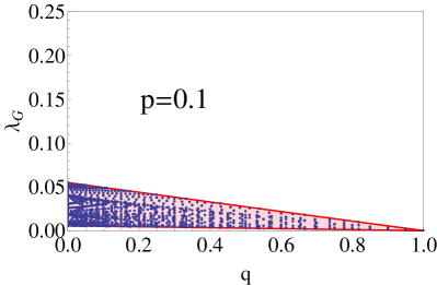
Figure 6: (Color online) Illustration of the dependance of the minimal eigenvalue $\lambda_{G}$ of operator $G$ on the parameter $q$ depicted for different values of the remaining parameters $s,\alpha,\beta,\gamma,\theta$ and $p$.

For this reason it is useful to plot $\lambda_{G}$ as a function of $q$ for some choice of remaining parameters (see Fig. 6). By numerically analyzing the actual dependence of the graphs on the parameters $s,\alpha,\beta,\gamma,\theta$ we observed that for a fixed $q$ the minimum and the maximum value of $\lambda_{G}$ can be achieved only when $s=1/(1+q)$ and $\theta=0$; $\theta=\pi/2$, respectively. In such case parameters $\alpha,\beta$ and $\gamma$ do not influence $\lambda_{G}$ and it can be calculated analytically. The obtained dependencies $G_{min}(p,q)$ and $G_{max}(p,q)$ are visualized on Fig. 6 as red lines, which form the boundary of the area where $\lambda_{G}$, the minimal eigenvalue of $G$, lies for any possible choice of its parameters. We can show that the minimum of $G_{min}(p,q)$ is zero and it is achieved only for $q=1$ corresponding to a unitary channel $\mathcal{F}$. Similarly, all the blue points in the Fig. 6 corresponding to the minimal eigenvalue of $G$ for some choice of its parameters were having $\lambda_{G}>0$, which proves that $G\geq 0$ in the considered range of parameters $q,s,\alpha,\beta,\gamma,\theta$. In conclusion, we proved that the boundariness is indeed achieved for decompositions containing at least one unitary channel, thus, it reads $b({\cal E}_{p})=p(1-p)$.

References

- (1) A. S. Holevo, Probabilistic and Statistical Aspects of Quantum Theory, North-Holland series in statistics and probability 1, (Amsterdam-New York-Oxford, 1982)
- (2) C. W. Helstrom, Quantum Detection and Estimation Theory, (Academic Press Inc., New York, 1976)
- (3) G. M. D’Ariano, P. Lo Presti, and P. Perinotti, Classical randomness in quantum measurements, J. Phys. A: Math. Gen. 38, 5979 (2005)
- (4) A. Jenčová, Base norms and discrimination of generalized quantum channels, J. Math. Phys. 55, 022201 (2014), [arXiv:1308.4030v1]
- (5) D. Reeb, M. J. Kastroyano and M. M. Wolf, Hilbert’s projective metric in quantum information theory, J. Math. Phys. 52, 082201 (2011), [arXiv:1102.5170]
- (6) T.Heinosaari and M. Ziman, The Language of Quantum Theory, (Cambridge University Press, 2013)
- (7) G. Chiribella, G. M. D’Ariano, and P. Perinotti, Theoretical framework for quantum networks, Phys. Rev. A 80, 022339 (2009), [arXiv:0904.4483v2]
- (8) Mark. M. Wilde, Quantum Information Theory, (Cambridge University Press, 2013)
- (9) J. Watrous, Semidefinite programs for completely bounded norms. Theory of Computing, 5(11), (2009)
- (10) G. Gutoski, On a measure of distance for quantum strategies, J. Math. Phys. 53, 032202 (2012), [arXiv:1008.4636v4]
- (11) C. D. Aliprantis and K. C. Border, Infinite Dimensional Analysis, A Hitchhiker’s Guide, Springer-Verlag, Berlin, Heidelberg (2006), 3rd edition
- (12) S. P. Eveson, Hilbert’s projective metric and the spectral properties of positive linear operators, Proc. London Math. Soc. 70 411-440 (1995),
- (13) Stephane Gaubert, Zheng QU, Dobrushin ergodicity coefficient for Markov operators on cones, and beyond, arXiv:1302.5226
- (14) M. Raginsky, Radon-Nikodým derivatives of quantum operations, J. Math. Phys. 44, 5003-5020 (2003)
- (15) P. Busch and S. P. Gudder, Effects as functions on projective Hilbert space, Lett. Math. Phys. 47, 329-337 (1999),
- (16) N. Hadjisavvas, Properties of mixtures on non-orthogonal states, Lett. Math. Phys. 5, 327-332 (1981),