Tomography by Fourier synthesis

Abstract

We consider a particular approach to the regularization of the inverse problem of computerized tomography. This approach is based on notions pertaining to Fourier synthesis. It refines previous contributions, in which the preprocessing of the data was performed according to the Fourier slice theorem. Since real models must account for the geometrical system response and possibly Compton scattering and attenuation, the Fourier slice theorem does not apply, yielding redefinition of the preprocessing. In general, the latter is not explicit, and must be performed numerically. The most natural choice of preprocessing involves the computation of unstable solutions. A proximal strategy is proposed for this step, which allows for accurate computations and preserves global stability of the reconstruction process.

Warning. This paper was submitted to the Journal of Inverse and Ill-Posed Problems on May 10, 2010, accepted there on November 28, 2010, and however never published.

1 Introduction

From the mathematical viewpoint, tomography consists in solving an ill-posed operator equation of the form $Rf_{0}=g$, where $f_{0}$ is the unknown image, $R$ is a linear operator (a simplified version of which being the Radon transformation) and $g$ is the data provided by the imaging device (e.g. a SPECT or PET camera). The data $g$ is usually referred to as the sinogram.

In the ideal model, $R$ is the standard Radon operator, given by

$$(Rf)(\boldsymbol{\theta},r)=\int f(\mathbf{x})\delta(r-\left\langle\boldsymbol{\theta},\mathbf{x}\right\rangle)\,\mathrm{d}\mathbf{x}.$$ (1)

Here, $\boldsymbol{\theta}=(\cos\phi,\sin\phi)$ is an element of the unit circle in $\mathds{R}^{2}$, $r$ is a real variable and $\delta$ denotes the Dirac delta function, so that the above integral is in fact the (one-dimensional) integral of $f$ over the line determined by the equation $r=\left\langle\boldsymbol{\theta},\mathbf{x}\right\rangle$. In this case, the celebrated Fourier Slice Theorem allows for considering the constraints on $f_{0}$ imposed by the equation $Rf_{0}=g$ as constraints on the Fourier transform of $f_{0}$, these constraints appearing on a radial domain of the Fourier plane. This observation led the authors of [8, 9] to regularize the ill-posed operator equation by means of concepts pertaining to Fourier synthesis [5].

Recall that Fourier synthesis refers to the generic problem of recovering a function $f_{0}$ from a partial and approximate knowledge of its Fourier transform. In [5], the analysis of spectral properties of the truncated Fourier operator led the authors to introduce a regularization principle which can be regarded as a reformulation into a well-posed problem of Fourier interpolation. The original problem of recovering the unknown object is replaced by that of recovering a limited resolution version of it, namely, $\phi_{\beta}\ast f_{0}$, where $\phi_{\beta}$ is some convolution kernel (or point spread function). In [1], inspired by well-known results from the approximation of $L^{p}$-functions by means of mollifiers, the authors established variational results for this type of regularization. They regarded $\phi_{\beta}$ as a member of the one-parameter family $\left\{\phi_{\beta}|\vphantom{\phi_{\beta}\beta\in\mathds{R}_{+}^{*}}\beta\in\mathds{R}_{+}^{*}\right\}$ defined by

$$\phi_{\beta}(\mathbf{x}):=\frac{1}{\beta^{2}}\phi\left(\frac{\mathbf{x}}{\beta}\right),$$

and studied the behavior of the reconstructed object as $\beta$ goes to zero.

Notice that mollifiers were also considered in [6]. By writing the mollified function $f_{\beta}:=\phi_{\beta}\ast f$ as

$$f_{\beta}(\mathbf{x}):=\int\phi_{\beta}(\mathbf{x}-\mathbf{y})f(\mathbf{y})\,\mathrm{d}\mathbf{y}=\left\langle\varphi_{\beta}(\mathbf{x},\cdot),f\right\rangle,$$

with $\varphi_{\beta}(\mathbf{x},\mathbf{y}):=\phi_{\beta}(\mathbf{x}-\mathbf{y})$, the duality associated to the underlying inner product is used to approximate $f_{\beta}$ via

$$f_{\beta}(\mathbf{x})\simeq\left\langle R^{*}\psi_{\beta}(\mathbf{x}),f\right\rangle=\left\langle\psi_{\beta}(\mathbf{x}),Rf\right\rangle,$$

in which $\psi_{\beta}(\mathbf{x})\simeq(R^{*})^{-1}\varphi_{\beta}(\mathbf{x},\cdot)$. This approach is referred to as the method of approximate inverses.

Our approach inherits features from both Fourier synthesis and the approximate inverses. In Section 2, we give a precise description of our methodology in a discrete setting. We shall focus on the problem of Computed Tomography. We shall introduce the notion of pseudo-commutant of a matrix with respect to another. In section 3, we discuss various computational strategies, especially concerning what we call preprocessing of the data, which consists in applying the aformentioned pseudo-commutant. Finally, in Section 4, we prove the numerical feasibility of our approach by means of reconstructions in emission tomography, in which the evolution towards realistic projectors made it necessary to give up the mere application of the Fourier Slice Theorem. Our numerical experiments will clearly indicate improvement in terms of stability and image quality.

2 A reconstruction methodology

As outlined in the introduction, our aim is to reconstruct a smoothed version $\phi_{\beta}\ast f_{0}$ of the original object $f_{0}$. Recall that, if the operator modelling data acquisition is actually the Radon operator $R$ defined in Equation (1), it is easy to generate the data corresponding to $\phi_{\beta}\ast f_{0}$. As a matter of fact, it results immediately from the Fourier Slice Theorem that

$$R(\phi_{\beta}\ast f_{0})=R\phi_{\beta}\circledast Rf_{0},$$ (2)

where $\circledast$ denotes the convolution with respect to $r$. If $g$ is an approximation of $Rf_{0}$, then $R\phi_{\beta}\circledast g$ will be an approximation of $R(\phi_{\beta}\ast f_{0})$. In terms of operators, this amounts to the existence of an operator $\Phi_{\beta}$ such that $RC_{\beta}=\Phi_{\beta}R$, where $C_{\beta}$ is the convolution operator: $C_{\beta}f:=\phi_{\beta}\ast f$. Now, realistic models describing the data acquisition in emission or transmission tomography involve operators which are not the exact Radon transformation, and which do not satisfy, in general, Equation (2).

In a recent paper [2], an extension of the regularization by mollification was proposed, in order to cope with operators $R$ for which it is not possible to explicitly find an operator $\Phi_{\beta}$ such that $RC_{\beta}=\Phi_{\beta}R$. The idea consists in defining $\Phi_{\beta}$ as an operator minimizing

$$X\mapsto\left\|RC_{\beta}-XR\right\|,$$

where $\left\|\cdot\right\|$ is some operator norm. In [2], the authors focus on the infinite dimensional setting, while considering general operators. Here, we concentrate on the discrete case. Therefore, from now on, $R$, $C_{\beta}$ and $X$ are matrices of respective sizes $m\times n$, $n\times n$ and $m\times m$, and we shall deal with the minimization of the Frobenius norm the matrix $RC_{\beta}-XR$ (with respect to $X$).

Recall that the Frobenius norm of a matrix $M\in\mathds{R}^{m\times n}$, denoted by $\left\|M\right\|_{F}$, is the Euclidean norm of $M$ regarded as a vector in $\mathds{R}^{mn}$, and that the corresponding inner product, denoted by $\left\langle\cdot,\cdot\right\rangle_{F}$, satisfies:

$$\forall M,N\in\mathds{R}^{m\times n},\quad\left\langle M,N\right\rangle_{F}=\mathop{\mathrm{tr}}(MN^{\top})=\mathop{\mathrm{tr}}(N^{\top}M).$$

The following theorem can be found in various sources and various forms. We provide a proof for the sake of completeness. Recall that a matrix $X\in\mathds{R}^{n\times m}$ is the pseudo-inverse $M^{\dagger}$ of $M$ if and only if it satisfies $MXM=M$, $XMX=X$, $(MX)^{\top}=MX$ and $(XM)^{\top}=XM$.

Theorem 2.1

Let $A$ and $R$ be real matrices of size $m\times n$. Then the matrix $AR^{\dagger}$ minimizes the function $f(X):=\left\|A-XR\right\|_{F}^{2}/2$ over $\mathds{R}^{m\times m}$. Among all minimizers, it is the one with minimum Frobenius norm.

Proof. Clearly, $f$ is convex, indefinitely differentiable, and its gradient at $X$ is equal to $(XR-A)R^{\top}$. Therefore,

$$\nabla f(AR^{\dagger})=A(R^{\dagger}RR^{\top}-R^{\top})=A\big{(}(RR^{\dagger}R)^{\top}-R^{\top}\big{)}=0.$$

This proves that $AR^{\dagger}$ minimizes $f$. Furthermore, since the Frobenius norm is strictly convex, minimizers of $f$ can only differ by matrices in the kernel of the linear mapping $\mathscr{R}\colon X\mapsto XR$ (from $\mathds{R}^{m\times m}$ to $\mathds{R}^{m\times n}$). Now, for all $K\in\mathds{R}^{m\times m}$,

$$\left\langle AR^{\dagger},K\right\rangle_{F}=\mathop{\mathrm{tr}}\big{(}AR^{\dagger}RR^{\dagger}K^{\top}\big{)}=\mathop{\mathrm{tr}}\big{(}AR^{\dagger}(R^{\dagger})^{\top}(KR)^{\top}\big{)}.$$

This implies that every matrix $K$ in the kernel of $\mathscr{R}$ is orthogonal (for $\left\langle\cdot,\cdot\right\rangle_{F}$) to $AR^{\dagger}$. The desired conclusion follows by Pythagoras’ theorem.  

Now, letting $A$ be the matrix $RC_{\beta}$, we see that the minimum Frobenius norm minimizer of the matrix function $X\mapsto\left\|RC_{\beta}-XR\right\|_{F}$ is the matrix

$$\Phi_{\beta}:=RC_{\beta}R^{\dagger}\in\mathds{R}^{m\times m}.$$

In order to be as consistent as possible with our aim, that is, with the reconstruction of the convolution of the original image by our point spread function $\phi_{\beta}$, we must replace the original sinogram with its transformation by $RC_{\beta}R^{\dagger}$.

Let $\mathbf{f}$ and $\mathbf{g}$ denote the discrete versions of $f$ and $g$, respectively. Consider the decomposition of the generic image $\mathbf{f}$ as the sum of its low and high frequency components:

$$\mathbf{f}=C_{\beta}\mathbf{f}+(I-C_{\beta})\mathbf{f}.$$

We define the reconstructed image as the solution to the following optimization problem:

$$(\mathscr{P})\quad\left|\begin{array}[]{rl}\hbox{Minimize}&\displaystyle\frac{1}{2}\left\|RC_{\beta}R^{\dagger}\mathbf{g}-R\mathbf{f}\right\|^{2}+\frac{\alpha}{2}\left\|H_{\beta}\mathbf{f}\right\|^{2}\\[6.45831pt] \hbox{subject to}&\mathbf{f}\geq\mathbf{0},\end{array}\right.$$

in which $\alpha$ is a positive weight and $H_{\beta}:=I-C_{\beta}$. From the computational viewpoint, the difficult part is the estimation of the regularized data $RC_{\beta}R^{\dagger}\mathbf{g}$. The reason is, of course, the ill-posedness of the model matrix $R$, which yields ill-posedness of the computation of $R^{\dagger}\mathbf{g}$. This difficulty will be addressed in the next section.

3 Computational aspects

In this section, we address the computation of the regularized data, that is, of $RC_{\beta}R^{\dagger}\mathbf{g}$. The resolution of problems such as $(\mathscr{P})$ is quite standard, and will not be discussed here.

Due to the dimension of the involved matrices, it seems unreasonable to actually compute either $RC_{\beta}R^{\dagger}$ or $R^{\dagger}$. The most natural strategy consists in computing $R^{\dagger}\mathbf{g}$ as the (unstable) minimum norm least square solution of the original system, and then in applying $RC_{\beta}$ to the obtained solution.

It may seem inappropriate to initialize a regularization scheme by computing an unstable solution. It is important, however, to realize that ill-posedness encompasses two aspects (which are related): the numerical inaccuracy induced by the poor conditioning of the system, and the propagation of measurement errors $\delta\mathbf{g}$. We conjecture, at this point, that the former can be dealt with by means of a proximal strategy, while the latter is not crucial since the unstable solution $R^{\dagger}\mathbf{g}$ is post-processed by the smoothing operator $C_{\beta}$ (and ultimately by $R$). In essence, the proximal point algorithm is a fixed point method. The reason for choosing an iterative scheme which, incidentally, has the reputation of being slow, is that it can give very accurate solutions. In fact, it may be used for refining solutions provided by some other method.

In the next paragraph, we review a few aspects of the Proximal Point Algorithm (PPA), applied to the computation of minimum norm least square solutions.

The Proximal Point Algorithm was introduced by Martinet [10] in 1970, in the context of variational inequalities. It was then generalized by Rockafellar [12] to the computation of zeros of maximal monotone operators (a particular case of which being the minimization of a convex function). In our context, that of computing the minimum norm least-square solution of the linear system $R\mathbf{f}=\mathbf{g}$, the PPA consists in the following steps:

• Initialization: put $k=0$ and choose an initial point $\mathbf{f}_{0}\in\mathds{R}^{n}$.

• Iteration: form the sequence $(\mathbf{f}_{k})_{k\geq 0}$ according to

  $$\mathbf{f}_{k+1}:=\mathop{\mathrm{argmin}}_{\mathbf{f}\in\mathds{R}^{n}}\left\{\frac{1}{2}\left\|\mathbf{g}-R\mathbf{f}\right\|^{2}+\frac{1}{2\lambda_{k}}\left\|\mathbf{f}-\mathbf{f}_{k}\right\|^{2}\right\},$$

  where $(\lambda_{k})_{k\geq 0}$ is a sequence of positive real numbers.

Observe that the function to be minimized in the iteration is strictly convex, smooth and coercive, and differs from the Tikhonov functional only by the subtraction of $\mathbf{f}_{k}$ in the regularizing part. It has the numerical stability inherent to Tikhonov regularization, and may be computed by using any routine from either quadratic optimization (e.g. the conjugate gradients) or linear algebra (on the corresponding regularized normal equation).

In [12], Rockafellar obtained convergence results for the proximal point algorithm, in the general setting of the computation of zeros of maximal monotone operators in real Hilbert spaces. For the sake of simplicity, we restrict attention to the minimization of any lower semi-continuous convex function on $\mathds{R}^{n}$. The proof of the following theorem is differed to the appendix.

Theorem 3.1

Let $F\colon\mathds{R}^{n}\to(-\infty,\infty]$ be a lower semi-continuous convex function which is not identically equal to infinity and bounded below, and let $\mathbf{x}_{0}$ be any point in $\mathds{R}^{n}$. Consider the sequence $(\mathbf{x}_{k})_{k\in\mathds{N}}$ defined by

$$\mathbf{x}_{k+1}=\mathop{\mathrm{argmin}}\left\{F(\mathbf{x})+\frac{1}{2\lambda_{k}}\left\|\mathbf{x}-\mathbf{x}_{k}\right\|^{2}|\vphantom{F(\mathbf{x})+\frac{1}{2\lambda_{k}}\left\|\mathbf{x}-\mathbf{x}_{k}\right\|^{2}\mathbf{x}\in\mathds{R}^{n}}\mathbf{x}\in\mathds{R}^{n}\right\},$$

where $(\lambda_{k})_{k\in\mathds{N}}$ is a sequence of positive numbers. If the series $\sum\lambda_{k}$ is divergent, then

$$F(\mathbf{x}_{k})\to\eta:=\inf\left\{F(\mathbf{x})|\vphantom{F(\mathbf{x})\mathbf{x}\in\mathds{R}^{n}}\mathbf{x}\in\mathds{R}^{n}\right\}\quad\hbox{as}\quad k\to\infty.$$

If in addition the set of minimizers $S:=\left\{\mathbf{x}\in\mathds{R}^{n}|\vphantom{\mathbf{x}\in\mathds{R}^{n}F(\mathbf{x})=\eta}F(\mathbf{x})=\eta\right\}$ is nonempty, then the sequence $(\mathbf{x}_{k})_{k\in\mathds{N}}$ converges to a point $\overline{\mathbf{x}}$ in $S$.

Now, let $F$ be the function $\mathbf{f}\mapsto\left\|\mathbf{g}-R\mathbf{f}\right\|^{2}/2$. In this case, the set $S$ of minimizers is the affine manifold

$$S=\left\{\mathbf{f}\in\mathds{R}^{n}|\vphantom{\mathbf{f}\in\mathds{R}^{n}R^{\top}R\mathbf{f}=R^{\top}\mathbf{g}}R^{\top}R\mathbf{f}=R^{\top}\mathbf{g}\right\}=\{R^{\dagger}\mathbf{g}\}+\mathop{\mathrm{ker}}R.$$

Furthermore, writing the usual first order necessary optimality condition for $\mathbf{f}_{k+1}$ yields

$$\mathbf{f}_{k+1}-\mathbf{f}_{k}=-\lambda_{k}R^{\top}(R\mathbf{f}_{k+1}-\mathbf{g})\in\mathop{\mathrm{ran}}R^{\top}=(\mathop{\mathrm{ker}}R)^{\perp}.$$

This shows that, if $\mathbf{f}_{0}=\mathbf{0}$, the limit point of the sequence $(\mathbf{f}_{k})_{k\in\mathds{N}}$ is nothing but $R^{\dagger}\mathbf{g}$ itself.

Notice that, in the case where $R$ is injective, the set of minimizers of $\left\|R\mathbf{f}-\mathbf{g}\right\|$ is reduced to the singleton $\{R^{\dagger}\mathbf{g}\}=\{(R^{\top}R)^{-1}R^{\top}\mathbf{g}\}$. In this case, numerical errors in the proximal iteration are unimportant, since each new iterate can be regarded as a new initial point. However, if $R$ is not injective, a component in the kernel of $R$ may grow due to finite precision in the iteration. In order to cope with this difficulty, the following strategy may be adopted. In practice, the smoothing properties of $RC_{\beta}$ are expected to give rise to reasonable perturbation transmission: a small perturbation $\delta\mathbf{f}\in\mathds{R}^{n}$ will yield a reasonably small perturbation $RC_{\beta}\delta\mathbf{f}\in\mathds{R}^{m}$. Therefore, replacing $R^{\dagger}$ with the usual Tikhonov approximation $(R^{\top}R+\varepsilon I)^{-1}R^{\top}$, where $I$ denotes the identity matrix of appropriate dimension and $\varepsilon$ is a very small positive parameter, will give a reasonable approximation of the regularized data:

$$RC_{\beta}(R^{\top}R+\varepsilon I)^{-1}R^{\top}\mathbf{g}\approx RC_{\beta}R^{\dagger}\mathbf{g}.$$

In the above proximal scheme, the iterations should then be replaced by

$$\mathbf{f}_{k+1}:=\mathop{\mathrm{argmin}}_{\mathbf{f}\in\mathds{R}^{n}}\left\{\frac{1}{2}\left\|\mathbf{g}-R\mathbf{f}\right\|^{2}+\frac{\varepsilon}{2}\left\|\mathbf{f}\right\|^{2}+\frac{1}{2\lambda_{k}}\left\|\mathbf{f}-\mathbf{f}_{k}\right\|^{2}\right\},$$

which will clearly yield convergence to $(R^{\top}R+\varepsilon I)^{-1}R^{\top}\mathbf{g}$.

We stress that mathematical convergence is guaranteed whenever the series $\sum\lambda_{k}$ is divergent, and that this happens in particular if $\lambda_{k}\equiv\lambda$ with $\lambda>0$. Notice that the smaller $\lambda_{k}$, the smaller the size of the step $\mathbf{f}_{k+1}-\mathbf{f}_{k}$. Consequently, it may be appropriate to start the algorithm with large values of $\lambda_{k}$ yielding large (but poorly conditioned) steps, and then let $\lambda_{k}$ decrease in order to have smaller but well-conditioned steps. Moreover, as indicated in [7], numerical accuracy in early iterations may be irrelevant: what really matters is the limit of the proximal sequence. We terminate this section with a few comments.

(1) If the size of $R$ is not prohibitively large, the computation of $R^{\dagger}$ may be performed by means of the singular value decomposition (SVD). The problems of tomographic reconstruction encountered in practice make it difficult or even impossible to perform the SVD. Approximate pseudo-inverses may then be obtained by truncating the SVD. Such approximate solution may be used as initial points for the PPA.

(2) As observed in [7], the proximal iteration with constant sequence $\lambda_{k}\equiv\lambda$ belongs to the class of fixed point methods, along with the algorithms of Jacobi, Gauss-Seidel, SOR and SSOR. It is easy to check that $R^{\dagger}\mathbf{g}$ satisfies the fixed point equation $\mathbf{f}=h(\mathbf{f})$, with

$$h(\mathbf{f}):=B\mathbf{f}+\mathbf{c},\quad B:=(I+\lambda R^{\top}R)^{-1}\quad\hbox{and}\quad\mathbf{c}:=\lambda(I+\lambda R^{\top}R)^{-1}R^{\top}\mathbf{g}.$$

Clearly, $h$ is a contraction and, if $R$ is injective, then $R^{\top}R$ is positive definite and $h$ is a strict contraction.

4 Numerical results

We now illustrate our reconstruction approach by a few numerical simulation. To begin with, we use a $64\times 64$ image of the Shepp-Logan phantom, as shown in Figure 1. The sinogram is obtained by means of an operator $R$ which accounts for the geometrical system response, as described in [3, 11] (the resolution in the projection depends on the distance to the detector). The simulated acquisition was performed with 64 bins and 64 angular values evenly spaced over 360 degrees. An independent Poisson noise was added to the sinogram, with parameter equal to the pixel value. (The total number of counts in the noisy sinogram is equal to 50065.)

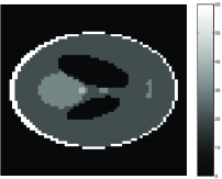
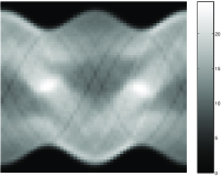
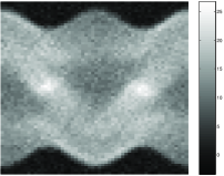
Figure 1: The shepp-Logan phantom (left), the corresponding sinogram (middle) and the noisy sinogram (right).

The reconstructions shown in Figure 2 were obtained by solving Problem $(\mathscr{P})$. The data is preprocessed according to the strategy described in the previous section. For comparison, reconstructions without preprocessing of the data are shown.

In practice, the positivity constraint can often be neglected: removing it from problem $(\mathscr{P})$ turns out to give images which are essentially positive. The advantage of this is that we deal with purely quadratic optimization, which allows for stability analysis as well as the use of the backward error stopping criterion, as in [9]: the reconstructions are performed using the conjugate gradients algorithm, with construction of the Galerkin tridiagonal matrix.

It is clear that preprocessing enhances the quality of the reconstruction. These simulations corroborate the anticipated relevance of our approach, and attests its numerical feasibility. It is interesting to note that, as conjectured in Section 3, the unstable step consisting in computing $R^{\dagger}\mathbf{g}$ does not damage the whole process: the application of $C_{\beta}$ to $R^{\dagger}\mathbf{g}$ is sufficient to ensure stability of the reconstruction.

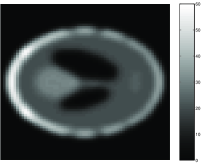
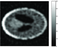
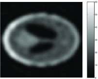
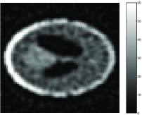
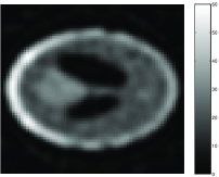
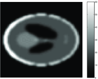
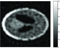
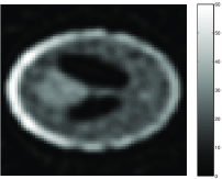
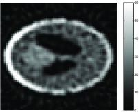
Figure 2: Images in the left column are mere convolutions of the original phantom image by the objective point-spread function (here a Hann filter is used), with cutoff frequency equal, in Nyquist units, to 0.5 (first line), 0.6 (second line), 0.7 (third line) and 0.8 (last line). The second and third columns show the corresponding reconstructions, respectively without and with preprocessing of the data.

Table 3 displays the normalized quadratic error

$$\mathscr{E}(\mathbf{f}):=\frac{\left\|C_{\beta}\mathbf{f}_{0}-\mathbf{f}\right\|}{\left\|C_{\beta}\mathbf{f}_{0}\right\|}$$

for various solutions $\mathbf{f}$: in the first line, $\mathbf{f}$ is reconstructed without preprocessing of the data, while in the second line, $\mathbf{f}$ is obtained without preprocessing. In the last line, the value (given for reference) is that corresponding to the reconstruction by Filtered Back-Projection (FBP). Here, $\mathbf{f}_{0}$ denotes the original object.

	Cutoff frequency
	0.5	0.6	0.7	0.8
without preprocessing	0.347786	0.301052	0.287429	0.291660
with preprocessing	0.118515	0.140563	0.168467	0.202067
with FBP	0.868203	0.879254	0.887703	0.891690

Figure 3: Normalized quadratic error $\mathscr{E}(\mathbf{f})$ for various cutoff frequencies and three reconstruction methods: Fourier synthesis without and with preprocessing (respectively first and second lines), and the Filtered Back-Projection (last line).

5 Conclusion

We have considered an extension of the regularization by mollification of the problem of computerized tomography. This was motivated by the fact that realistic models differ from the standard Radon transform: the latter cannot be used if the system response accounts for geometrical aspects as well as Compton scattering and attenuation.

The data corresponding to the objective of our reconstruction process (namely a smoothed version of the original object) can be computed numerically by means of the proximal point algorithm, which operates even when the dimension of the system matrix makes it difficult or impossible to use the SVD.

Simulations have shown both the numerical feasibility of our regularization scheme and its efficiency, in terms of robustness and image quality. The unstable computation of the pseudo-inverse of the data fits in a regularization strategy without affecting its global stability.

Such a strategy may be used to apply the regularization by mollification to many other imaging techniques. More generally, the proximal algorithm may provide the user with an efficient tool for preprocessing the data in accordance with the objective of the reconstruction, whenever the latter objective is a linear transform of the original image.

6 Appendix: proof of Theorem 3.1

We start with a finite dimensional version of Opial’s lemma:

Lemma 6.1

Let $(\mathbf{x}_{k})_{k\in\mathds{N}}$ be an $\mathds{R}^{n}$-valued sequence, and let $S$ be a nonempty subset of $\mathds{R}^{n}$. Suppose that

• for all $\mathbf{x}\in S$, the sequence $(\left\|\mathbf{x}_{k}-\mathbf{x}\right\|)_{k\in\mathds{N}}$ has a limit;

• every cluster point of $(\mathbf{x}_{k})$ belongs to $S$.

Then $(\mathbf{x}_{k})$ converges to a point $\overline{\mathbf{x}}$ in $S$.

Proof. Condition (i) implies that $(\mathbf{x}_{k})$ is bounded, which implies in turn that the sequence has at least one cluster point, say $\overline{\mathbf{x}}$. We shall prove that every cluster point $\check{\mathbf{x}}$ must coincide with $\overline{\mathbf{x}}$. Let $(\mathbf{x}_{k_{j}})_{j\in\mathds{N}}$ be a subsequence converging to $\overline{\mathbf{x}}$ and $(\mathbf{x}_{k^{\prime}_{j}})_{j\in\mathds{N}}$ be a subsequence converging to $\check{\mathbf{x}}$. Condition (ii) implies that both $\overline{\mathbf{x}}$ and $\check{\mathbf{x}}$ belong to $S$. Condition (i) again implies that

$$\left\|\mathbf{x}_{k}-\overline{\mathbf{x}}\right\|^{2}-\left\|\mathbf{x}_{k}-\check{\mathbf{x}}\right\|^{2}$$

has a limit. Developing the above expression then shows that the sequence $\left\langle\mathbf{x}_{k},\overline{\mathbf{x}}-\check{\mathbf{x}}\right\rangle$ has a limit, from which we deduce that

$$\lim_{j\to\infty}\big{\langle}\mathbf{x}_{k_{j}},\overline{\mathbf{x}}-\check{\mathbf{x}}\big{\rangle}=\lim_{j\to\infty}\big{\langle}\mathbf{x}_{k^{\prime}_{j}},\overline{\mathbf{x}}-\check{\mathbf{x}}\big{\rangle}.$$

Therefore, $\left\langle\overline{\mathbf{x}},\overline{\mathbf{x}}-\check{\mathbf{x}}\right\rangle=\left\langle\check{\mathbf{x}},\overline{\mathbf{x}}-\check{\mathbf{x}}\right\rangle$, which immediately yields $\overline{\mathbf{x}}=\check{\mathbf{x}}$.  

Recall that the effective domain of a convex function $F$ is defined to be the set

$$\mathop{\mathrm{dom}}F:=\left\{\mathbf{x}\in\mathds{R}^{n}|\vphantom{\mathbf{x}\in\mathds{R}^{n}F(\mathbf{x})<\infty}F(\mathbf{x})<\infty\right\},$$

and that the subdifferential of $F$ at a point $\mathbf{x}$ is the (closed convex) set

$$\partial F(\mathbf{x}):=\left\{\boldsymbol{\xi}\in\mathds{R}^{n}|\vphantom{\boldsymbol{\xi}\in\mathds{R}^{n}\forall\mathbf{y}\in\mathds{R}^{n},\;F(\mathbf{y})\geq F(\mathbf{x})+\left\langle\boldsymbol{\xi},\mathbf{y}-\mathbf{x}\right\rangle}\forall\mathbf{y}\in\mathds{R}^{n},\;F(\mathbf{y})\geq F(\mathbf{x})+\left\langle\boldsymbol{\xi},\mathbf{y}-\mathbf{x}\right\rangle\right\}.$$

Members $\boldsymbol{\xi}$ of the subdifferential are called subgradients, and the inequality in the definition of $\partial F(\mathbf{x})$ is referred to as the subgradient inequality.

Proof of theorem 3.1. For all $\mathbf{x}\in\mathds{R}^{n}$,

$$F(\mathbf{x}_{k+1})+\frac{1}{2\lambda_{k}}\left\|\mathbf{x}_{k+1}-\mathbf{x}_{k}\right\|^{2}\leq F(\mathbf{x})+\frac{1}{2\lambda_{k}}\left\|\mathbf{x}-\mathbf{x}_{k}\right\|^{2}.$$

Taking $\mathbf{x}=\mathbf{x}_{k}$ yields

$$F(\mathbf{x}_{k+1})+\frac{1}{2\lambda_{k}}\left\|\mathbf{x}_{k+1}-\mathbf{x}_{k}\right\|^{2}\leq F(\mathbf{x}_{k}).$$

This shows that the sequence $F(\mathbf{x}_{0}),F(\mathbf{x}_{1}),\ldots$ decreases, and since $F$ is bounded below, the sequence converges to some real limit $l\geq\eta:=\inf\left\{F(\mathbf{x})|\vphantom{F(\mathbf{x})\mathbf{x}\in\mathds{R}^{n}}\mathbf{x}\in\mathds{R}^{n}\right\}$. In order to obtain the first assertion of the theorem, we must prove that actually $l=\eta$. We start by proving the following inequality:

$$\forall\mathbf{x}\in\mathop{\mathrm{dom}}F,\quad\left\|\mathbf{x}_{k}-\mathbf{x}\right\|^{2}-\left\|\mathbf{x}_{k+1}-\mathbf{x}\right\|^{2}\geq 2\lambda_{k}\big{(}F(\mathbf{x}_{k+1})-F(\mathbf{x})\big{)}.$$ (3)

The optimality of $\mathbf{x}_{k+1}$ reads:

$$\mathbf{0}\in\partial F(\mathbf{x}_{k+1})+\frac{\mathbf{x}_{k+1}-\mathbf{x}_{k}}{\lambda_{k}},$$

that is, $\mathbf{x}_{k}-\mathbf{x}_{k+1}\in\lambda_{k}\partial F(\mathbf{x}_{k+1})$. In other words, there exists $\boldsymbol{\xi}$ in $\partial F(\mathbf{x}_{k+1})$ such that $\mathbf{x}_{k}-\mathbf{x}_{k+1}=\lambda_{k}\boldsymbol{\xi}$. Now, for all $\mathbf{x}\in\mathop{\mathrm{dom}}F$, we have:

$$\left\|\mathbf{x}_{k}-\mathbf{x}\right\|^{2}$$

$$= \left\|\mathbf{x}_{k}-\mathbf{x}_{k+1}\right\|^{2}+\left\|\mathbf{x}_{k+1}-\mathbf{x}\right\|^{2}+2\left\langle\mathbf{x}_{k}-\mathbf{x}_{k+1},\mathbf{x}_{k+1}-\mathbf{x}\right\rangle$$

$$\geq \left\|\mathbf{x}_{k+1}-\mathbf{x}\right\|^{2}+2\left\langle\mathbf{x}_{k}-\mathbf{x}_{k+1},\mathbf{x}_{k+1}-\mathbf{x}\right\rangle$$

$$= \left\|\mathbf{x}_{k+1}-\mathbf{x}\right\|^{2}+2\lambda_{k}\left\langle\boldsymbol{\xi},\mathbf{x}_{k+1}-\mathbf{x}\right\rangle$$

$$\geq \left\|\mathbf{x}_{k+1}-\mathbf{x}\right\|^{2}+2\lambda_{k}\big{(}F(\mathbf{x}_{k+1})-F(\mathbf{x})\big{)},$$

in which the last inequality stems from the subgradient inequality. Thus (3) is clear. Next, since $F(\mathbf{x}_{k+1})\geq l$ for all $k$, (3) implies that

$$\forall\mathbf{x}\in\mathop{\mathrm{dom}}F,\quad\left\|\mathbf{x}_{k}-\mathbf{x}\right\|^{2}-\left\|\mathbf{x}_{k+1}-\mathbf{x}\right\|^{2}\geq 2\lambda_{k}\big{(}l-F(\mathbf{x})\big{)}.$$

Summing the above for $k=0,\ldots,n$ shows that, for all $\mathbf{x}\in\mathop{\mathrm{dom}}F$,

$$\left\|\mathbf{x}_{0}-\mathbf{x}\right\|^{2}-\left\|\mathbf{x}_{n+1}-\mathbf{x}\right\|^{2}\geq 2\left(\sum_{k=0}^{n}\lambda_{k}\right)\big{(}l-F(\mathbf{x})\big{)}.$$

Since the series $\sum\lambda_{k}$ is divergent, we must have $l\leq F(\mathbf{x})$ for all $\mathbf{x}\in\mathop{\mathrm{dom}}F$, which eventually show that $l\leq\eta$.

It remains to prove that, assuming $S:=\mathop{\mathrm{argmin}}F\not=\emptyset$, the proximal sequence $(\mathbf{x}_{k})$ converges to a point $\overline{\mathbf{x}}\in S$. Since $F(\mathbf{x}_{k+1})-F(\mathbf{x})\geq 0$ for every $\mathbf{x}\in S$, (3) shows that

$$\forall\mathbf{x}\in S,\quad\left\|\mathbf{x}_{k}-\mathbf{x}\right\|^{2}\geq\left\|\mathbf{x}_{k+1}-\mathbf{x}\right\|^{2}.$$

Thus $\left\|\mathbf{x}_{k}-\mathbf{x}\right\|$ decreases as $k$ increases, which obviously implies that $\left\|\mathbf{x}_{k}-\mathbf{x}\right\|$ goes to a limit. It follows that the sequence $(\mathbf{x}_{k})$ is bounded. Now, by lower semi-continuity, every cluster point $\overline{\mathbf{x}}$ of $(\mathbf{x}_{k})$ (there is at least one since the sequence is bounded) satisfies

$$F(\overline{\mathbf{x}})\leq\lim_{j\to\infty}F(\mathbf{x}_{k_{j}})=\lim_{k\to\infty}F(\mathbf{x}_{k})=l.$$

Thus every cluster point of $(\mathbf{x}_{k})$ belongs to $S$, and Opial’s lemma shows that the sequence $(\mathbf{x}_{k})$ actually converges to a point $\overline{\mathbf{x}}$ in $S$.

References

• [1] N. Alibaud, P. MarΓ©chal and Y. Saesor, A variational approach to the inversion of truncated Fourier operators, Inverse Problems 25, 2009.
• [2] X. Bonnefond and P. MarΓ©chal, A variational approach to the inversion of some compact operators, Pacific Journal of Optimization 5(1), pp. 97-110.
• [3] A.R. Formiconi, A. Pupi, A. Passeri, Compensation of spatial system response in SPECT with conjugate gradient reconstruction technique, Phys. Med. Biol. 34, pp. 69-84, 1989.
• [4] P. M. Koulibaly, I. Buvat, M. Pelegrini and G. El fakhri, Correction de la perte de rΓ©solution avec la profondeur, Revue de l’ACOMEN, 4, pp. 114-120, 1998.
• [5] A. Lannes, S. Roques and M.-J. Casanove, Stabilized reconstruction in signal and image processing; Part I: partial deconvolution and spectral extrapolation with limited field, J. Mod. Opt. 34, pp. 161-226, 1987.
• [6] A.K. Louis and P. Maass, A mollifer method for linear operator equations of the first kind, Inverse Problems 6, pp. 427-440, 1990.
• [7] P. MarΓ©chal, A. Rondepierre, A proximal approach to the inversion of ill-conditioned matrices, C. R. Acad. Sci. Paris, Ser. I 347, pp. 1435-1438, 2009.
• [8] P. MarΓ©chal, D. Togane and A. Celler, A new reconstruction methodology for computerized tomography: FRECT (Fourier Regularized Computed Tomography), IEEE, Trans. Nucl. Sc., 47, pp. 1595-1601, 2000.
• [9] D. Mariano-Goulart, P. MarΓ©chal, L. Giraud, S. Gratton and M. Fourcade, A priori selection of the regularization parameters in emission tomography by Fourier synthesis, Computerized Medical Imaging and Graphics, 31, pp. 502-509, 2007.
• [10] B. Martinet, RΓ©gularisation d’inΓ©quations variationelles par approximations successives, Revue FranΓ§aise d’Informatique et de Recherche OpΓ©rationelle, pp. 154-159, 1970.
• [11] A. Passeri, A.R. Formiconi and U. Meldolesi, Physical modelling (geometrical system response, Compton scattering and attenuation) in brain SPECT using the conjugate gradient reconstruction method, Phys. Med. Biol., 37, pp. 1727-1744, 1992.
• [12] R.T. Rockafellar, Monotone operators and the proximal point algorithm, SIAM Journal on Control and Optimization, 14 (5), pp.877-898, 1976.