Optimal Control of Effective Hamiltonians

Abstract

We present a systematic scheme for optimization of quantum simulations. Specifically, we show how polychromatic driving can be used to significantly improve the driving of Raman transitions in the Lambda system, which opens new possibilities for controlled driven-induced effective dynamics.

In the past few years, one of the most active and promising research fields has been the design of quantum simulators, i.e. engineered controllable quantum systems utilized to mimic the dynamics of other systems. With this, new insight is expected to be gained in a variety of phenomena like high-temperature fractional quantum Hall states Tang et al. (2011), (non-)abelian gauge fields Hauke et al. (2012); Banerjee et al. (2013) and even relativistic effects Goldman et al. (2009); Franco-Villafañe et al. (2013).

Driven systems provide a powerful tool to simulate desired effective dynamics. An important example are laser-assisted Raman transitions between different electronic states and/or localized states of trapped atoms, which is a central pillar in a large number of quantum simulations. Because the direct coupling between low-lying energy states via dipole transitions is often forbidden by selection rules, an intermediate auxiliary state with higher energy is usually used to mediate the coupling. This so-called Lambda system is then specifically configured to imprint phases required to realize various spin-orbit couplings Cheuk et al. (2012); Wang et al. (2012) or to simulate the effect of gauge fields Miyake et al. (2013); Aidelsburger et al. (2013). Other prominent examples of driving-induced effective dynamics include shaken lattices Eckardt et al. (2005); Lignier et al. (2007); Struck et al. (2012), lattices with modulated interactions Rapp et al. (2012) or driven graphene Iadecola et al. (2013).

Even though driven systems provide a powerful approach to perform quantum simulations, they often rely on approximations that currently situate them still far from the ideal quantum simulator. For instance, in Raman transitions via a three-level Lambda system, the driving pulse produces an undesired population of the excited state. These deviations between the desired and simulated dynamics accumulate during the evolution and become considerable after a sufficiently long time. From the experimental side, however, spectacular progress has been made in the manipulation and control of quantum systems Braun et al. (2013); Struck et al. (2013), so that accurate theoretical tools to choose the proper driving are necessary. The field of optimal control theory D’Alessandro (2007); Krotov (1996) aims at such precise manipulation but, so far, it has primarily targeted properties at single instances in time Khaneja et al. (2005); Reich et al. (2013); Bartels and Mintert (2013) whereas we are rather concerned with the behavior of a system during a continuous time window.

In this Letter, we provide a general systematic approach to improve quantum simulations by using pulse shaping techniques of optimal control theory. We discuss in detail the optimal control of the Lambda system and rigorously show how an appropriately chosen polychromatic driving can significantly improve Raman transitions. As a result, we do not only provide a proof of principle for the optimal control of effective Hamiltonians but also optimize a building-block used in a large variety of quantum simulations.

Consider the target dynamics $U_{\rm tg}=e^{-iH_{\rm tg}t}$, generated by the target Hamiltonian $H_{\text{tg}}$ that we wish to simulate using a time-periodic driving Hamiltonian $H(t)=H(t+T)$. Its time–evolution operator $U(t)=\mathcal{T}\exp[-i\int_{0}^{t}H(t^{\prime})dt^{\prime}]$ then admits the Floquet decomposition Floquet (1883)

$$U(t)=\tilde{U}(t)U_{\text{eff}}(t).$$ (1)

Here $\tilde{U}(t)$ is a $T$-periodic unitary satisfying $\tilde{U}(0)=\mathbbm{1}$, $U_{\text{eff}}(t)=e^{-iH_{\text{eff}}t}$ and $H_{\text{eff}}$ is a time-independent effective Hamiltonian defined via $U(T)=e^{-iH_{\text{eff}}T}$. $\tilde{U}$ describes fluctuations around the envelope evolution $U_{\text{eff}}$. These fluctuations become negligible if typical matrix elements $\Omega_{\text{eff}}$ of $H_{\text{eff}}$ are sufficiently small compared to the driving frequency $\omega=2\pi/T$. In this case the low-energy or long-time dynamics of the periodically driven system is well described by $H_{\text{eff}}$, which in turn should be chosen to match the target Hamiltonian $H_{\text{tg}}$ to be simulated. Suppose now that the driving $H(t)$ contains a set $\{f_{n}\}$ of control parameters. Our aim is to tune these parameters such that the dynamics $U$ resembles the target dynamics $U_{\rm tg}$ as well as possible. Different choices of $\{f_{n}\}$ can result in similar effective dynamics, but produce different fluctuations. In order to ensure the optimal simulation of a given target Hamiltonian $H_{\rm tg}$ with least fluctuations, our scheme therefore consists in:

(i) Identifying the dependence of the effective Hamiltonian $H_{\text{eff}}$ on the control parameters $\{f_{n}\}$. Typically this can only be achieved in an approximate manner, where $H_{\text{eff}}=\sum_{k=0}^{r}H_{\text{eff}}^{(k)}+O(\Omega_{\rm eff}\epsilon^{r+1})$ is known up to order $r$ of the small parameter $\epsilon=\Omega_{\text{eff}}/\omega\ll 1$.

(ii) Constraining $\{f_{n}\}$ so that $H_{\text{tg}}=H_{\text{eff}}$ to the same order $r$.

(iii) Minimizing the target functional

$$\mathcal{F} = \dfrac{1}{T}\int_{0}^{T}\|U(t)-U_{\text{tg}}(t)\|^{2}dt,$$ (2)

where $||\cdot||^{2}={\rm\textrm{Tr}\left(\cdot^{\dagger}\cdot\right)}$ is the Hilbert–Schmidt norm, under the constrained control parameters allowed by (ii). $\mathcal{F}$ shall also be approximated to the order $r$ consistent with (i-ii).

In order to calculate $H_{\text{eff}}$, $U(t)$, and $\mathcal{F}$, we use the Magnus expansion Magnus (1954); Blanes et al. (2009) and write $U(t)=e^{-iM(t)}$ as the exponential of a time-dependent operator $M(t)=\sum_{k=1}^{\infty}M_{k}(t)$. The first two terms of this series are $M_{1}(t)=\int_{0}^{t}H(t_{1})dt_{1}$ and

$$M_{2}(t) = -\dfrac{i}{2}\int_{0}^{t}dt_{1}\int_{0}^{t_{1}}dt_{2}[H(t_{1}),H(t_{2})].$$ (3)

The $k$th-order Magnus operator $M_{k}(t)$ contains $k$-fold time integrals of $k-1$ nested commutators. When $H(t)$ is $T$-periodic, $M_{k}(T)$ is exactly of order $\epsilon^{k}$. Thus, $H_{\text{eff}}^{(k)}=M_{k+1}(T)/T$, since the factor $1/T$ reduces the order of expansion by one. In this manner, $H_{\text{eff}}$, $U(t)$, and consequently $\mathcal{F}$ are determined up to order $r$, and our scheme (i-iii) yields parameters $\{f_{n}\}$ that ensure the optimal simulation of $H_{\text{tg}}$.

In the following, we exemplify the method described above with a case study of the degenerate Lambda system where $|1\rangle$ and $|2\rangle$ denote the two ground states and $|3\rangle$ the excited state. The target Hamiltonian

$$H_{\text{tg}}=-\Omega_{\text{tg}}\left(|1\rangle\langle 2|+|2\rangle\langle 1|\right)$$ (4)

generates Raman transitions within the ground-state manifold at a rate $\Omega_{\text{tg}}$ (the overall sign is chosen for later convenience). Our aim is to simulate this dynamics by driving the transitions $|1\rangle\leftrightarrow|3\rangle$ and $|2\rangle\leftrightarrow|3\rangle$ with a suitably modulated Rabi frequency. In the interaction picture, where the dynamics induced by the static Hamiltonian is absorbed in the state vectors, the driving Hamiltonian takes the form

$$H(t) = f(t)\left(1+e^{-in_{0}\Delta t}\right)\left(|1\rangle\langle 3|+|2\rangle\langle 3|\right)+\text{H.c.}.$$ (5)

Importantly, we assume that the driving pulse

$$f(t)=\sum_{n=1}^{N}f_{n}e^{-in\omega t}$$ (6)

is written as a general Fourier series in terms of $\omega$, the fundamental frequency of driving. Since we do not want the optimization to rely on strong intensity and fast frequencies, the maximal frequency in the above pulse is the detuning $\Delta=\epsilon_{3}-\omega_{d}=N\omega$ between the driving carrier and excitation frequency. In other words, no Fourier components with frequency larger than $\Delta$ need to be generated. $H(t)$ defined in Eq. (5) should be periodic with period $T=2\pi/\omega$, which is the case if $\Delta$ is a fraction of twice the driving carrier frequency, such that $n_{0}$ is a integer. In the rotating wave approximation, one would neglect the counter-rotating contribution $e^{-in_{0}\Delta t}$ in (5); we consider the general case and keep this term.

Let us first discuss the simplest example of a monochromatic (MC) driving $f(t)=f_{1}e^{-i\Delta t}$ at constant Rabi frequency by taking $N=1$ in eq. (6). Since the Magnus operator $M_{2l}(t)$ of even order contains even products of $H(t)$, the corresponding effective Hamiltonian $H_{\rm eff}^{(2l-1)}$ has the desired structure of $H_{\text{tg}}$ with matrix elements that couple the ground states . Choosing

$$|f_{1}|^{2}=\Omega_{\text{tg}}\Delta\frac{1+n_{0}}{2+n_{0}},$$ (7)

the constraint $H_{\text{eff}}^{(1)}=H_{\text{tg}}$ can be fulfilled to first order since $H_{\text{eff}}^{(0)}=0$. The second-order term $H_{\rm eff}^{(2)}$, on the other hand, will generate undesired transitions to the upper level via cubic powers of $H(t)$. With $f_{1}$ already fixed, one cannot impose $H_{\text{eff}}^{(2)}=0$, so that one always ends up with an unwanted population in the excited state—except in the ideal limit of very strong, far-detuned driving $|f_{1}|,\Delta\rightarrow\infty$ at fixed $\Omega_{\text{tg}}$. Thus, with only one frequency, one can neither accurately realize the desired unitary ground-state dynamics nor simultaneously minimize the fluctuations.

Let us then take advantage of the general pulse (6) and implement the first constraint $H_{\text{eff}}^{(1)}=H_{\text{tg}}$ with

$$\Omega_{\text{tg}} = \dfrac{1}{\omega}\sum_{n=1}^{N}\dfrac{|f_{n}|^{2}}{\tilde{n}(1)},$$ (8)

where $\tilde{n}(p)^{-1}\equiv n^{-p}+(n+Nn_{0})^{-p}$. [In the rotating wave approximation $n_{0}\to\infty$ this simplifies to $\tilde{n}(p)=n^{p}$.] Pushing the Magnus expansion to third order, we can now require $H_{\text{eff}}^{(2)}=0$ through the second constraint

$$0 = \sum_{n=1}^{N}\dfrac{f_{n}}{\tilde{n}(1)}.$$ (9)

The target functional to be minimized reads

$$\mathcal{F}^{\left(2\right)}=\frac{4}{\omega^{2}}\sum_{n=1}^{N}\dfrac{|f_{n}|^{2}}{\tilde{n}(2)}.$$ (10)

We can solve the optimization problem now analytically by introducing two Lagrange multipliers $\lambda_{1}\in\mathbbm{R},\lambda_{2}\in\mathbbm{C}$ for the two constraints (8) and (9), respectively. The optimal pulse parameters are found to be

$$f_{n} = \omega\lambda_{2}\left(\dfrac{\tilde{n}(1)}{\tilde{n}(2)}-\lambda_{1}\right)^{-1}.$$ (11)

The Lagrange multipliers are determined by inserting this solution into the constraints (8) and (9). Dividing eq. (11) by $\lambda_{2}$ shows that $f_{n}/\lambda_{2}$ is real, and thus all $f_{n}$ as well as $\lambda_{2}$ can be taken real. Using Eqs. (8) and (9), the target functional (10) can be rewritten as $\mathcal{F}^{(2)}=4\lambda_{1}\Omega_{\text{tg}}/\omega$, such that the global minimum of the fluctuations is found with the minimal root $\lambda_{1}$ of Eq. (9) with (11) inserted. One should be able to suppress fluctuations more efficiently using more frequencies, and indeed, as $N\to\infty$ the minimal $\lambda_{1}$ tends to $\tilde{N}(1)/\tilde{N}(2)\sim 1/N$, such that $\mathcal{F}^{(2)}\rightarrow 0$.

With relatively little effort, one can take the calculation one step further. Using the first 4 terms of the Magnus expansion, the constraint (8) can be extended to third order $H^{(1)}_{\rm eff}+H^{(3)}_{\rm eff}=H_{\rm tg}$ with the constraint

$$\Omega_{\text{tg}} = \omega\left(A_{1}+2B_{3}-4A_{1}A_{2}\right)$$ (12)

defined in terms of $A_{p}=\sum|f_{n}/\omega|^{2}/\tilde{n}(p)$ and $B_{p}=\sum|f_{n}/\omega|^{4}/\tilde{n}(p)$. Eq. (10) does not change to this order since $\mathcal{F}^{(3)}=0$. The optimal Fourier components $\{f_{n}\}$ can still be chosen real and solve the coupled system of equations ($n=1,...,N$)

$$\frac{f_{n}}{\omega}\left[\dfrac{1+4A_{1}\lambda_{1}}{\tilde{n}(2)}-\lambda_{1}\dfrac{1-4A_{2}}{\tilde{n}(1)}\right]-\dfrac{4\lambda_{1}f_{n}^{3}}{\tilde{n}(3)\omega^{3}}=\dfrac{\lambda_{2}}{\tilde{n}(1)}.$$ (13)

(a) (b)

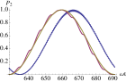
(c)

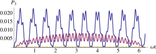
Figure 1: (color online). (a) and (b) Transition probability $P_{2}(t)=|\langle 2|U(t)|1\rangle|^{2}$ for the target dynamics (yellow), MC dynamics (blue) and third-order optimal dynamics with $N=10$ frequency components (red). (c) Population of the excited state $P_{3}=|\langle 3|U(t)|1\rangle|^{2}$ as a function of time. Plot parameters are $\Omega_{\text{tg}}=0.05\omega$ and $n_{0}=4$.

The full minimization in third order of expansion, given by the system of equations (13), (9) and (12), can be straightforwardly solved using the exact second-order solution (11) as an initial condition for a numerical routine. Fig. 1 shows the dynamics over one driving period and illustrates the striking advantages of polychromatic (PC) driving with $N=10$ frequencies over the MC dynamics. First of all, because of the approximative identification $H_{\rm eff}\approx H_{\rm tg}$, the effective dynamics always shows a systematic drift with respect to the target dynamics. In panels (a) and (b) of Fig. 1, the evolution over a single driving period is compared for short and long times, respectively. While the MC evolution with Rabi frequency (7) deviates significantly from the target evolution after several driving periods, the optimal PC dynamics follows the target rather faithfully. As the amplitude of the MC pulse has been chosen in first order, one might wonder if a better performance can be realized with an effective Hamiltonian that includes higher orders. Such a construction, however, would require a higher driving amplitude and, since the undesired terms in $H_{\text{eff}}^{(2)}$ cannot be set to zero, it results in larger overall deviations with respect to the target dynamics. Thus an improvement of the MC case is not possible through a more accurate treatment. The lower panel (c) of Fig. 1 shows the second main advantage, namely significantly smaller fluctuations of the optimal dynamics around the target dynamics and, in particular, a considerably lower population of the intermediate (excited) state.

\begin{overpic}[scale={.5},unit=1mm]{TF.pdf} \put(22.0,15.0){\includegraphics[scale={.4}]{FourierComponentsBRWA.pdf}} \end{overpic}

Figure 2: Magnitude of fluctuations, quantified by eq. (10), around the target unitary dynamics simulated by a third-order optimal pulse, as function of the number of modulation Fourier components; plot parameters are $\Omega_{\text{tg}}=0.05\omega$ and $n_{0}=4$. Inset: Fourier components for $N=10$.

In order to show how much the fluctuations can be suppressed, Fig. 2 plots the resulting third-order target fidelity $\mathcal{F}\approx\sum_{k=0}^{3}\mathcal{F}^{\left(k\right)}=\mathcal{F}^{\left(2\right)}$ of eq. (10), as a function of the number $N$ of frequency components. Clearly, already a moderate number of frequency components permits to reduce the fluctuations dramatically. The Fourier components of the optimal pulse for $N=10$ are shown in the inset. The component $f_{10}$ of the highest frequency $\Delta=10\omega$ is close to the MC solution (7); lower frequency components are phase-shifted by $\pi$ and their magnitude decays rapidly with decreasing frequency. These results show that modulating the driving with only few frequencies suffices to simulate the desired target unitary with significantly higher precision than in the MC case.

The long-time deviations observed in Fig. 1(b) can be quantitatively measured by the target functional $\mathcal{F}_{n}$, as defined in Eq. (2), but integrated over the $n$th driving period. In Fig. 3, these fidelities are shown for the MC pulse and the second- and third-order PC pulses with $N=10$ as function of $n$. Let us first compare the MC with the second-order PC pulse. In the first few periods, the optimized solution indeed yields a better result. However, the deviations with respect to the target dynamics grow faster in the second order optimized case than in the MC case. As a consequence, in the long-time regime the MC driving performs better than the optimized solution calculated in second order: since the PC pulse contains slower frequencies than the MC one, the expansion at second order leads to a worse approximation of the effective Hamiltonian and the deviations between $U_{\rm eff}$ and $U_{\rm tg}$ accumulate in time and overcome the difference in fluctuations after a sufficiently long times. Indeed, we observe that the larger $N$ is, the later the crossover occurs, since the fluctuations are smaller and deviations from the target Hamiltonian need more time to accumulate to the value of the MC dynamics. Nevertheless, the optimized PC pulse can always be systematically improved by pushing the calculations to higher order in the expansion parameter. As seen in Figs. 1 as well as 3, the third order optimal pulse significantly outperforms the MC dynamics in the entire time domain.

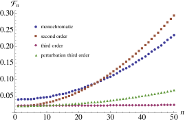
Figure 3: (color online). Deviations from the target dynamics $\mathcal{F}_{n}$ in the $n$th driving period for the MC pulse (blue circles), the second-order optimized pulse (brown squares) and the third-order optimized pulse (red rhombi) with $N=10$. The perturbed third order solution [see Eq. (14)] with frequency randomness $\delta=\delta_{\text{max}}/4$, averaged over 100 realizations (green triangles), shows good resilience against experimental uncertainty. $\Omega_{\text{tg}}=0.05\omega$ and $n_{0}=4$.

Finally, in order to estimate the robustness of optimal pulses in realistic experimental setups, we investigate how small perturbations to the Fourier components affect the performance of the optimal pulses. Consider perturbations of the form

$$f_{n}\rightarrow\tilde{f}_{n}=f_{n}+\delta{f}$$ (14)

where $\delta f$ is a random number uniformly distributed in the interval $[-\delta,\delta]$, which accounts for the experimental uncertainty in the tuned Fourier components. Comparison between the second- and third-order optimal pulses shows that their largest optimal Fourier components differ typically by $0.01\omega$ (for $\Omega_{\text{tg}}=0.05\omega$), which defines a scale $\delta_{\text{max}}$ for the maximum allowed uncertainty. Perturbations with $\delta=\delta_{\text{max}}/4$, however, still lead to a good performance, see Figure 3. Thus, the optimal pulses appear robust under such perturbations, which indicates a good experimental viability.

The control of periodically driven systems by means of pulse shaping presented here opens new perspectives for the optimal simulation of quantum systems. No increase in intensity as compared to mono-chromatic driving is required and the realization of optimal effective Hamiltonians is robust under perturbations. The optimal pulses have a rather narrow spectral range, what eases the identification of driving parameters ensuring that no high lying states are excited. This is of particular importance for large many-body systems, like trapped atomic gases, where un-careful driving easily results in uncontrolled heating. Since this can be avoided with the present approach, it may, for example, be used to enhance or suppress long-range or density-dependent tunneling processes Verdeny et al. (2013) in shaken optical lattices.

Financial support by the European Research Council within the project ODYCQUENT is gratefully acknowledged. F.M. acknowledges hospitality by the Centre for Quantum Technologies, a Research Centre of Excellence funded by the Ministry of Education and the National Research Foundation of Singapore.

References

- Tang et al. (2011) E. Tang, J.-W. Mei, and X.-G. Wen, Phys. Rev. Lett. 106, 236802 (2011).
- Hauke et al. (2012) P. Hauke, O. Tieleman, A. Celi, C. Ölschläger, J. Simonet, J. Struck, M. Weinberg, P. Windpassinger, K. Sengstock, M. Lewenstein, and A. Eckardt, Phys. Rev. Lett. 109, 145301 (2012).
- Banerjee et al. (2013) D. Banerjee, M. Bögli, M. Dalmonte, E. Rico, P. Stebler, U.-J. Wiese, and P. Zoller, Phys. Rev. Lett. 110, 125303 (2013).
- Goldman et al. (2009) N. Goldman, A. Kubasiak, A. Bermudez, P. Gaspard, M. Lewenstein, and M. A. Martin-Delgado, Phys. Rev. Lett. 103, 035301 (2009).
- Franco-Villafañe et al. (2013) J. A. Franco-Villafañe, E. Sadurní, S. Barkhofen, U. Kuhl, F. Mortessagne, and T. H. Seligman, Phys. Rev. Lett. 111, 170405 (2013).
- Cheuk et al. (2012) L. W. Cheuk, A. T. Sommer, Z. Hadzibabic, T. Yefsah, W. S. Bakr, and M. W. Zwierlein, Phys. Rev. Lett. 109, 095302 (2012).
- Wang et al. (2012) P. Wang, Z.-Q. Yu, Z. Fu, J. Miao, L. Huang, S. Chai, H. Zhai, and J. Zhang, Phys. Rev. Lett. 109, 095301 (2012).
- Miyake et al. (2013) H. Miyake, G. A. Siviloglou, C. J. Kennedy, W. C. Burton, and W. Ketterle, Phys. Rev. Lett. 111, 185302 (2013).
- Aidelsburger et al. (2013) M. Aidelsburger, M. Atala, M. Lohse, J. T. Barreiro, B. Paredes, and I. Bloch, Phys. Rev. Lett. 111, 185301 (2013).
- Eckardt et al. (2005) A. Eckardt, C. Weiss, and M. Holthaus, Phys. Rev. Lett. 95, 260404 (2005).
- Lignier et al. (2007) H. Lignier, C. Sias, D. Ciampini, Y. Singh, A. Zenesini, O. Morsch, and E. Arimondo, Phys. Rev. Lett. 99, 220403 (2007).
- Struck et al. (2012) J. Struck, C. Ölschläger, M. Weinberg, P. Hauke, J. Simonet, A. Eckardt, M. Lewenstein, K. Sengstock, and P. Windpassinger, Phys. Rev. Lett. 108, 225304 (2012).
- Rapp et al. (2012) A. Rapp, X. Deng, and L. Santos, Phys. Rev. Lett. 109, 203005 (2012).
- Iadecola et al. (2013) T. Iadecola, D. Campbell, C. Chamon, C.-Y. Hou, R. Jackiw, S.-Y. Pi, and S. V. Kusminskiy, Phys. Rev. Lett. 110, 176603 (2013).
- Braun et al. (2013) S. Braun, J. P. Ronzheimer, M. Schreiber, S. S. Hodgman, T. Rom, I. Bloch, and U. Schneider, Science 339, 52 (2013).
- Struck et al. (2013) J. Struck, M. Weinberg, C. Olschlager, P. Windpassinger, J. Simonet, K. Sengstock, R. Hoppner, P. Hauke, A. Eckardt, M. Lewenstein, and L. Mathey, Nat Phys 9, 738 (2013).
- D’Alessandro (2007) D. D’Alessandro, Introduction to Quantum Control and Dynamics (CRC, Boca Raton, 2007).
- Krotov (1996) V. F. Krotov, Global Methods in Optimal Control Theory (Marcel Dekker, New York, 1996).
- Khaneja et al. (2005) N. Khaneja, T. Reiss, C. Kehlet, T. Schulte-Herbrüggen, and S. J. Glaser, J. Magn. Res. 172, 296 (2005).
- Reich et al. (2013) D. M. Reich, G. Gualdi, and C. P. Koch, Phys. Rev. Lett. 111, 200401 (2013).
- Bartels and Mintert (2013) B. Bartels and F. Mintert, Phys. Rev. A 88, 052315 (2013).
- Floquet (1883) G. Floquet, Ann. École Norm. Sup. 12, 47 (1883).
- Magnus (1954) W. Magnus, Comm. P. and App. Math. 7, 649 (1954).
- Blanes et al. (2009) S. Blanes, F. Casas, J. Oteo, and J. Ros, Phys. Rep. 470, 151 (2009).
- Note (1) These terms also generate light-shift displacements of the excited and ground states which do not influence the target dynamics between the two ground states.
- Verdeny et al. (2013) A. Verdeny, A. Mielke, and F. Mintert, Phys. Rev. Lett. 111, 175301 (2013).