H I, CO, and Planck/IRAS dust properties in the
high-latitude-cloud complex, MBM 53, 54, 55 (catalog ) and HLCG $92{-}35$ (catalog ); Possible evidence for an optically thick H I envelope
around the CO clouds

Abstract

We present an analysis of the H I and CO gas in conjunction with the Planck/IRAS sub-mm/far-infrared dust properties toward the most outstanding high latitude clouds MBM 53, 54, 55 (catalog ) and HLCG $92{-}35$ (catalog ) at $b={-}30^{\circ}$ to ${-}45^{\circ}$. The CO emission, dust opacity at $353\,\mathrm{GHz}$ ($\tau_{353}$), and dust temperature ($T_{\mathrm{d}}$) show generally good spatial correspondence. On the other hand, the correspondence between the H I emission and the dust properties is less clear than in CO. The integrated H I intensity $W_{\mbox{{\scriptsize H}{\tiny\,I}}}$ and $\tau_{353}$ show a large scatter with a correlation coefficient of $\sim 0.6$ for a $T_{\mathrm{d}}$ range from $16\,\mathrm{K}$ to $22\,\mathrm{K}$. We find however that $W_{\mbox{{\scriptsize H}{\tiny\,I}}}$ and $\tau_{353}$ show better correlation for smaller ranges of $T_{\mathrm{d}}$ every $0.5\,\mathrm{K}$, generally with a correlation coefficient of $0.7\mbox{--}0.9$. We set up a hypothesis that the H I gas associated with the highest $T_{\mathrm{d}}\geq 21.5\,\mathrm{K}$ is optically thin, whereas the H I emission is generally optically thick for $T_{\mathrm{d}}$ lower than $21.5\,\mathrm{K}$. We have determined a relationship for the optically thin H I gas between atomic hydrogen column density and $\tau_{353}$, $N_{\mbox{{\scriptsize H}{\tiny\,I}}}\,(\mathrm{cm^{-2}})=(1.5\times 10^{26})\cdot\tau_{353}$, under the assumption that the dust properties are uniform, and applied it to estimate $N_{\mbox{{\scriptsize H}{\tiny\,I}}}$ from $\tau_{353}$ for the whole cloud. $N_{\mbox{{\scriptsize H}{\tiny\,I}}}$ was then used to solve for $T_{\mathrm{s}}$ and $\tau_{\mbox{{\scriptsize H}{\tiny\,I}}}$ over the region. The result shows that the H I is dominated by optically thick gas having low spin temperature of $20\,\mathrm{K}\mbox{--}40\,\mathrm{K}$ and density of $40\,\mathrm{cm^{-3}}\mbox{--}160\,\mathrm{cm^{-3}}$. The H I envelope has a total mass of $\sim 1.2\times 10^{4}\,M_{\odot}$, an order of magnitude larger than that of the CO clouds. The H I envelope properties derived by this method do not rule out a mixture of H I and $\mbox{H}_{2}$ in the dark gas, but we present indirect evidence that most of the gas mass is in the atomic state.

1 Introduction

The neutral interstellar medium (ISM) consists of H I, $\mbox{H}_{2}$, and possibly “dark gas”, which is believed to be undetectable in line emission of H I or CO (Grenier et al., 2005; Planck Collaboration et al., 2011b). The H I emission at $21\,\mathrm{cm}$ wavelength and the CO emission at $2.6\,\mathrm{mm}$ offer tools to probe atomic and molecular hydrogen. The CO clouds have low kinetic temperature $10\,\mathrm{K}\mbox{--}100\,\mathrm{K}$ with density above $1000\,\mathrm{cm^{-3}}$ as derived by analyses of multi-$J$ CO transitions (e.g. Castets et al., 1990). The CO intensity is converted into molecular column density by an $X_{\mbox{\scriptsize CO}}$ factor, which is empirically determined by assuming dynamical equilibrium of the CO clouds, dust properties measured in extinction and/or far-infrared emission, and comparison with gamma rays created by proton-proton collisions via neutral pion decay (e.g., Blitz et al., 2007; Fukui & Kawamura, 2010; Bolatto et al., 2013). On the other hand, the physical parameters of the H I gas have been rather ambiguous, mainly because the H I emission has a single observed quantity, intensity as a function of velocity, for two independent variables spin temperature $T_{\mathrm{s}}$ and H I optical depth $\tau_{\mbox{{\scriptsize H}{\tiny\,I}}}$, not allowing us to determine each of these observationally. The H I consists of warm and cold components (for a review see Kalberla & Kerp, 2009; Dickey & Lockman, 1990). The mass of the H I gas having spin temperature higher than $\sim 100\,\mathrm{K}$ is measurable at reasonably high accuracy under the optically thin approximation, while the cold component having spin temperature of $20\,\mathrm{K}\mbox{--}80\,\mathrm{K}$ is measured by comparing the absorption and emission H I profiles only where background continuum sources are available (Dickey et al., 2003; Heiles & Troland, 2003). It is notable that some recent works on TeV gamma-ray supernova remnants show that the cold H I gas which is not detectable in CO at $1\,\sigma$ integrated intensity level of $\sim 1\,\mathrm{K\,km\,s^{-1}}$ (Fukui et al., 2012) is responsible for the gamma-rays via collision between cosmic-ray protons and interstellar protons (Fukui et al., 2012; Fukui, 2013; Fukuda et al., 2014). However, the observed sample of cold H I is limited and the cold H I still needs further effort to better constrain its physical properties.

Recent progress in measuring the infrared and sub-mm emission over the whole sky is remarkable. These observations are strongly motivated by the aim to precisely measure the cosmic microwave background (CMB) radiation and its polarization. In particular, the Planck collaboration released the whole sky distribution of dust temperature $T_{\mathrm{d}}$ and dust opacity $\tau_{353}$ at $5\,\mathrm{arcmin}$ resolution which have been achieved through sensitive measurements of the dust emission above $100\,\mathrm{GHz}$ in the Galactic foreground. Five papers of the Planck collaboration presented comparisons between CO and dust emission (Planck Collaboration et al., 2011b, e, d, c, f). These studies derived basic physical relationships between the neutral gas and the dust emission and concluded that the dark gas (Grenier et al., 2005) occupies $15\,\%$ of the interstellar medium (ISM), where the H I emission was assumed to be optically thin. Similar studies on $21\,\mathrm{cm}$ H I emission include Lee et al. (2012) and Planck Collaboration et al. (2011a).

The high latitude molecular clouds MBM 53, 54, 55 (catalog ) and HLCG $92{-}35$ (catalog ) are one of the largest cloud systems in the sky at Galactic latitude of ${-}30\,\mathrm{degree}\ \mbox{--}\ {-}50\,\mathrm{degree}$ with only minor background components (Magnani et al., 1985). The distance of the cloud system is determined to be $150\,\mathrm{pc}$ (Welty et al., 1989). Yamamoto et al. (2003) used the NANTEN $4\,\mathrm{m}$ telescope to observe the $J{=}1\mbox{--}0$ transitions of ${}^{12}\mbox{CO}$, ${}^{13}\mbox{CO}$, and $\mathrm{C}^{18}\mathrm{O}$ and mapped the molecular distribution. The velocity of the MBM 53, 54, 55 (catalog ) and HLCG $92{-}35$ (catalog ) clouds is mainly in range from ${-}11\,\mathrm{km\,s^{-1}}$ to $0\,\mathrm{km\,s^{-1}}$ for CO. The half-power beam widths were $2.6\,\mathrm{arcmin}\mbox{--}2.7\,\mathrm{arcmin}$ and their grid spacings are $4$ or $8\,\mathrm{arcmin}$ for the ${}^{12}\mbox{CO}$, $2\,\mathrm{arcmin}$ for the ${}^{13}\mbox{CO}$ and the $\mathrm{C}^{18}\mathrm{O}$. They also identified associated H I gas at $36\,\mathrm{arcmin}$ resolution and discussed that the H I gas is being converted into $\mbox{H}_{2}$ under the dynamical effect of a nearby shell driven by stellar winds. Gir et al. (1994) studied and identified the associated H I, while their coverage was limited to ${\sim}1/2$ of the area studied by Yamamoto et al. (2003). For reference, this region is rich in high latitude clouds including a far-infrared looplike structure in Pegasus, and Yamamoto et al. (2006) observed this loop in $\mbox{CO}(J{=}1\mbox{--}0)$ lines. MBM 53, 54, 55 (catalog ) and HLCG $92{-}35$ (catalog ) clouds show no sign of active star formation and are an ideal target to study detailed ISM properties under the general interstellar radiation field. The regions of the MBM 53, 54, 55 (catalog ) and HLCG $92{-}35$ (catalog ) clouds and the Pegasus loop have also been used to test CO component separation in the analysis of the cosmic microwave background emission (Ichiki et al., 2014).

In order to better understand the detailed physical properties of the local ISM, we have undertaken new $\mbox{CO}(J{=}1\mbox{--}0)$ observations of MBM 53, 54, 55 (catalog ) and HLCG $92{-}35$ (catalog ) in the on-the-fly mode with the $2.6\,\mathrm{arcmin}$ beam of the NANTEN2 $4\,\mathrm{m}$ telescope as part of the NANTEN Super CO survey (=NASCO), which is aiming to cover $70\,\%$ of the sky. By using the H I dataset at $4\,\mathrm{arcmin}$ resolution from the GALFA archive data, we have compared the CO and H I with the Planck/IRAS dust properties. In this paper we present the first results from the detailed comparison. Section 2 describes the observations, Section 3 gives the results and analysis, and Section 4 presents conclusions. Another paper which deals with the dust emission covering the whole sky will be published separately (Fukui et al., 2014) and is complementary to the present paper.

2 Observational datasets

In this study we used NANTEN2 CO data, GALFA H I data, the dust emission data measured by Planck/IRAS, and the $1.4\,\mathrm{GHz}$ radio continuum data. All the data are gridded to $1\,\mathrm{arcmin}$, smaller than the angular resolutions of these datasets.

2.1 CO data

${}^{12}\mbox{CO}(J{=}1\mbox{--}0)$ and ${}^{13}\mbox{CO}(J{=}1\mbox{--}0)$ emission were obtained by the NANTEN2 $4\,\mathrm{m}$ millimeter/submillimeter telescope of Nagoya University, which is installed at an altitude of $4865\,\mathrm{m}$ in northern Chile. Observations of the ${}^{12}\mbox{CO}(J{=}1\mbox{--}0)$ and ${}^{13}\mbox{CO}(J{=}1\mbox{--}0)$ lines were simultaneously conducted in several sessions from 2011 November to 2013 January, and cover about $75\,\mathrm{deg}^{2}$. Only observational parameters of ${}^{12}\mbox{CO}(J{=}1\mbox{--}0)$ are described below. The front end was a $4\,\mathrm{K}$ cooled Nb Superconductor-Insulator-Superconductor (SIS) mixer receiver, and the double-sideband (DSB) system temperature was $\sim 200\,\mathrm{K}$ including the atmosphere toward the zenith. The spectrometer was a digital Fourier transform spectrometer (DFS) with 16,384 channels, providing velocity resolution of $0.2\,\mathrm{km\,s^{-1}}$. All observations were conducted by using an on-the-fly (OTF) mapping technique with a $2.6\,\mathrm{arcmin}$ main beam at a $1\,\mathrm{arcmin}$ data sampling, and each spatial area of $1\,\mathrm{degree}$ by $1\,\mathrm{degree}$ was mapped several times in different scanning directions to reduce scanning effects by basket-weave technique (Emerson & Graeve, 1988). These OTF data were reduced into fits data cubes with the original idl software. The rms noise fluctuations in ${}^{12}\mbox{CO}(J{=}1\mbox{--}0)$ spectra after basket-weave technique were $\sim 1.2\,\mathrm{K}$ per channel in the main beam temperature, $T_{\mathrm{mb}}$. The CO data is smoothed to $5\,\mathrm{arcmin}$ spatial resolution to be compared with H I and Planck/IRAS datasets. The final rms noise fluctuations are $\sim 0.6\,\mathrm{K}$ per channel in a $5\,\mathrm{arcmin}$ smoothed beam. The pointing was checked regularly using planets, and the applied corrections were always smaller than $20\,\mathrm{arcsec}$. The standard sources M17 SW and Ori KL were observed for intensity calibration. The CO intensity is integrated over a velocity range from $-12\,\mathrm{km\,s^{-1}}$ to ${+}2\,\mathrm{km\,s^{-1}}$.

2.2 H I data

Archival datasets of the GALFA-H I survey are used (Peek et al., 2011). The survey was conducted on the Arecibo Observatory $305\,\mathrm{m}$ telescope and the angular resolution of the data is $4\,\mathrm{arcmin}$. The rms noise fluctuations of the H I data are $\sim 0.25\,\mathrm{K}$ per channel in $T_{\mathrm{mb}}$. The H I data are also smoothed to $5\,\mathrm{arcmin}$ resolution, and the rms noise fluctuations of the final H I spectra are $0.2\,\mathrm{K}$ per channel for the $5\,\mathrm{arcmin}$ beam. The H I intensity is spread over a velocity range from ${-}49\,\mathrm{km\,s^{-1}}$ to ${+}17\,\mathrm{km\,s^{-1}}$, while most of the H I emission is between ${-}25\,\mathrm{km\,s^{-1}}$ and ${+}12\,\mathrm{km\,s^{-1}}$.

2.3 Planck/IRAS data

Archival datasets of the optical depth at $353\,\mathrm{GHz}$ ($\tau_{353}$) and dust temperature ($T_{\mathrm{d}}$) were obtained by fitting $353$, $545$, and $857\,\mathrm{GHz}$ data of the first 15 months observed by the Planck satellite and $100\,\mathrm{micron}$ data measured by the IRAS satellite. Both of these data have angular resolutions of $5\,\mathrm{arcmin}$. For details, see the Planck Legacy Archive (PLA) explanatory supplement (Planck Collaboration, 2013).

2.4 Radio continuum data

As the $1.4\,\mathrm{GHz}$ radio continuum background we use the CHIPASS data (Calabretta et al., 2014) for the region at $\delta(\mathrm{J2000})<25^{\circ}$ and the data described in Reich (1982) and Reich & Reich (1986) for the region at $\delta(\mathrm{J2000})\geq 25^{\circ}$. Their spatial resolutions are $14.4\,\mathrm{arcmin}$ and $35\,\mathrm{arcmin}$, respectively. Although these data have lower angular resolutions than the rest analyzed in the study, the peak radiation temperature of the continuum data shows small variations from $\sim 3.4\,\mathrm{K}$ to $\sim 4.9\,\mathrm{K}$ except for the area within $\sim 30\,\mathrm{arcmin}$ of the quasar 3C 454.3, which happens to be located near the CO clouds (e.g., Abdo et al., 2011). We used these lower resolution data by excluding the area around 3C 454.3.

2.5 Masking

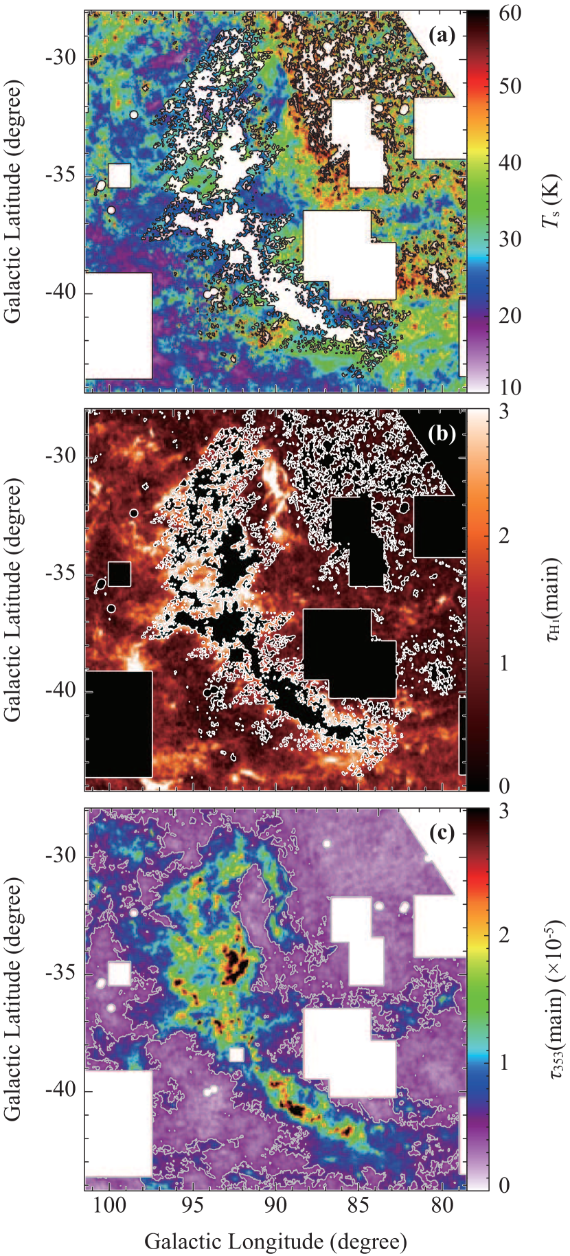
Figure 7: (a) and (b) show the spatial distribution of $T_{\mathrm{s}}$ and $\tau_{\mbox{{\scriptsize H}{\tiny\,I}}}(\mathrm{main})$ solved from the two equations (3) and (4) in the text. The masks described in Section 2.5. are applied, and in addition the areas where $T_{\mathrm{s}}\geq 70\,\mathrm{K}$ are masked. (c) represents the spatial distribution of $\tau_{353}(\mathrm{main})$. The gray contours indicate the level of $\tau_{353}(\mathrm{main})=5\times 10^{-6}$.

In the present analysis, the local interstellar medium toward the cloud system is approximated by a single layer. This is consistent with the velocity of the H I being peaked at around $0\,\mathrm{km\,s^{-1}}$, and generally a single velocity component is dominant. In order to eliminate possible sources of contamination, we further applied the following masking. These masked areas are listed in Table 1 (see also Figure 7).

• The areas showing CO emission higher than $1.1\,\mathrm{K\,km\,s^{-1}}$ ($1\sigma$) are masked in order to exclude the contribution of the CO-emitting molecular gas.

• The two regions where there is a secondary H I peak outside the velocity range from $-25\,\mathrm{km\,s^{-1}}$ to $+12\,\mathrm{km\,s^{-1}}$ are masked at $(\ell,b)\sim(81\fdg 5,-33\fdg 0)$, $(85\fdg 6,-33\fdg 8)$. Generally, these secondary peaks show intensity comparable to that of the main H I peak.

• Regions with high $T_{\mathrm{d}}$ indicating localized heating by stars etc. are masked by referring to the IRAS point source catalog etc. The most extended region of such high $T_{\mathrm{d}}$ is located toward 3C 454.3, although the origin of the high $T_{\mathrm{d}}$ is not known.

• The six regions where the H I data are missing are masked.

3 Results

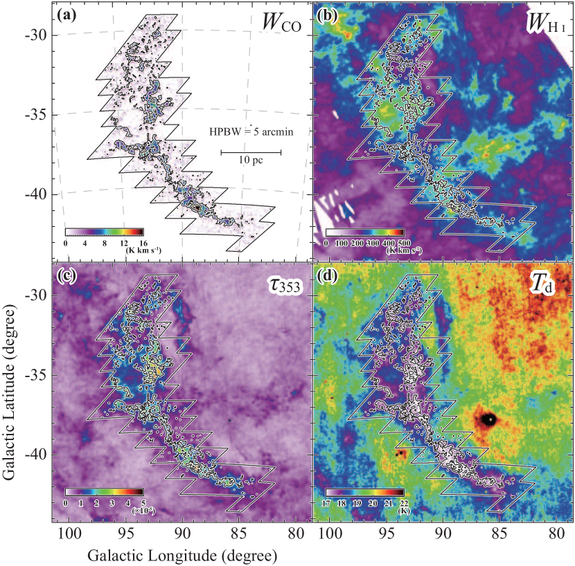
Figure 1: (a) Velocity-integrated intensity map of ${}^{12}\mbox{CO}(J{=}1\mbox{--}0)$ in the galactic coordinates. The integrated LSR-velocity range is from ${-}12\,\mathrm{km\,s^{-1}}$ to ${+}2\,\mathrm{km\,s^{-1}}$. The contours are drawn every $7.9\,\mathrm{K\,km\,s^{-1}}$ from $3.4\,\mathrm{K\,km\,s^{-1}}$. The bounding box shows the observed area. (b), (c), and (d) are spatial distributions of velocity-integrated intensity of the H I ($W_{\mbox{{\scriptsize H}{\tiny\,I}}}$), the optical depth at $353\,\mathrm{GHz}$ ($\tau_{353}$), and the temperature of the cold dust ($T_{\mathrm{d}}$), respectively. The contours of CO and the bounding boxes are the same as in (a). The integrated velocity range of the $W_{\mbox{{\scriptsize H}{\tiny\,I}}}$ in (b) is from ${-}49\,\mathrm{km\,s^{-1}}$ to ${+}17\,\mathrm{km\,s^{-1}}$. The effective beam sizes are $5\,\mathrm{arcmin}$ for the 4 panels.

Figure 1 shows four panels which present CO, H I and Planck/IRAS dust properties. Figure 1(a) shows the $\mbox{CO}(J{=}1\mbox{--}0)$ velocity integrated intensity distribution, $W_{\mbox{\scriptsize CO}}\,(\mathrm{K\,km\,s^{-1}})$. Figure 1(b) shows an overlay of H I and CO where we confirm the associated H I in the previous works (Gir et al., 1994; Yamamoto et al., 2003). $W_{\mbox{{\scriptsize H}{\tiny\,I}}}$ ($\mathrm{K\,km\,s^{-1}}$) is the intensity of H I integrated from ${-}49\,\mathrm{km\,s^{-1}}$ to ${+}17\,\mathrm{km\,s^{-1}}$. Figure 1(c) presents an overlay of $\tau_{353}$ and CO. The comparison shows good correspondence between them within the CO contours, whereas the correspondence of H I with $\tau_{353}$ seems less clear than in the case of CO. We note that $\tau_{353}$ is significantly extended beyond the lowest CO contour $3.4\,\mathrm{K\,km\,s^{-1}}$ ($3\,\sigma$). Figure 1(d) shows an overlay of $T_{\mathrm{d}}$ and CO. The lowest $T_{\mathrm{d}}\sim 16\,\mathrm{K}$ is clearly associated with CO, and $T_{\mathrm{d}}$ increases up to ${\sim}22\,\mathrm{K}$ outside the CO clouds.

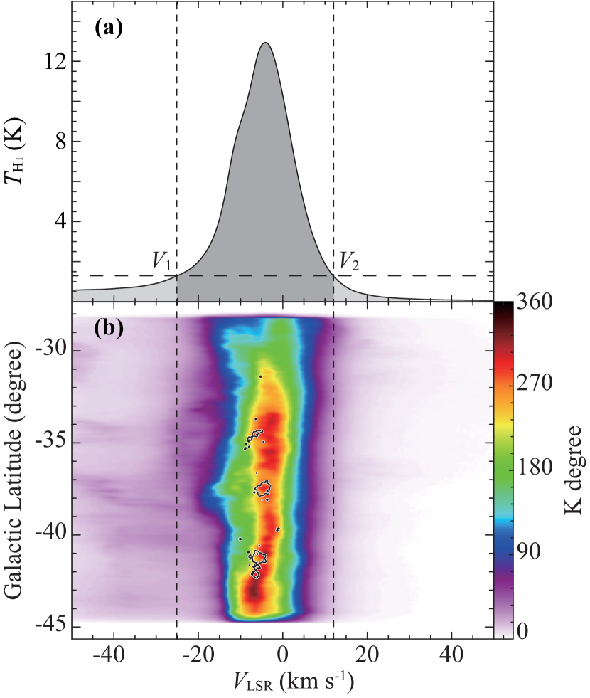
Figure 2: (a) Average spectrum of the H I in the region shown in Figure 1(d), but the masking described in Section 2.5. are applied. $T_{\mathrm{mb}}$ at $V_{1}={-}25\,\mathrm{km\,s^{-1}}$ and at $V_{2}={+}12\,\mathrm{km\,s^{-1}}$ correspond to $10\,\%$ level of the peak. (b) Latitude-velocity diagram of H I (color image) and CO (contours) integrated over the longitude range in Figure 1. The integrating range are from $\ell\sim 80^{\circ}$ to $\sim 100^{\circ}$. The level of the CO contours is $\sim 3\,\mathrm{K\,degree}$. $89\,\%$ of the H I emission is concentrated in the velocity range from $-25\,\mathrm{km\,s^{-1}}$ to $+12\,\mathrm{km\,s^{-1}}$.

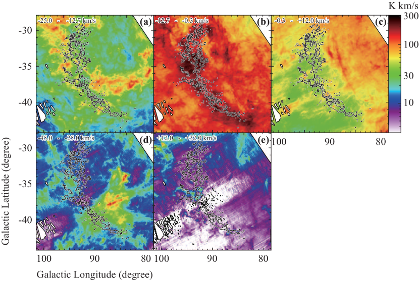
Figure 10: Velocity channel maps of the H I (color image) superposed on the $W_{\mbox{\scriptsize CO}}$ (contours). In panels (a), (b), and (c), we show the channel maps of the main H I cloud with dividing the velocity range into three. Panels (d) and (e) show the channel maps outside the main H I velocity range. The contour level of $W_{\mbox{\scriptsize CO}}$ is $3.4\,\mathrm{K\,km\,s^{-1}}$ for each panel.

Figure 2(a) where masking in Section 2.5. is applied shows an average H I spectrum over the region in Figure 1, and Figure 2(b), the H I integrated intensity over the same longitude range, where ${}^{12}\mbox{CO}(J{=}1\mbox{--}0)$ intensity is superposed by black contours. Figure 2(a) indicates that most of the H I emission is in the range from ${-}25\,\mathrm{km\,s^{-1}}$ to ${+}12\,\mathrm{km\,s^{-1}}$ which is determined by the $10\,\%$ level of the average H I spectrum and the H I emission from ${-}25\,\mathrm{km\,s^{-1}}$ to ${+}12\,\mathrm{km\,s^{-1}}$ has a single component, which includes $89\,\%$ of the H I integrated intensity. The remaining $11\,\%$ of the H I emission is mainly on the negative velocity side at $V_{\mathrm{LSR}}<-25\,\mathrm{km\,s^{-1}}$. In order to eliminate possible contamination of the H I at $V_{\mathrm{LSR}}<-25\,\mathrm{km\,s^{-1}}$ we shall adopt the H I velocity range from $-25\,\mathrm{km\,s^{-1}}$ to $+12\,\mathrm{km\,s^{-1}}$ in the following analysis and call this the main H I cloud. This velocity range includes the H I which has been suggested to be associated with the CO clouds (Gir et al., 1994; Yamamoto et al., 2003), and more details are given in Appendix A on the H I velocity channel distributions (Figure 10).

In the following, $\tau_{353}$ and $W_{\mbox{{\scriptsize H}{\tiny\,I}}}$ denote those quantities for the whole velocity range and $\tau_{353}(\mathrm{main})$ and $W_{\mbox{{\scriptsize H}{\tiny\,I}}}(\mathrm{main})$ for the main H I cloud only. The excluded velocity ranges from the main H I cloud have very weak H I intensity of $\lesssim 30\,\mathrm{K\,km\,s^{-1}}$ (Figure 2(b)) and it is likely that this H I is optically thin. $W_{\mbox{{\scriptsize H}{\tiny\,I}}}(\mathrm{main})$ is calculated from $W_{\mbox{{\scriptsize H}{\tiny\,I}}}$ by subtracting the H I integrated intensity at $V_{\mathrm{LSR}}<-25\,\mathrm{km\,s^{-1}}$ and $V_{\mathrm{LSR}}>+12\,\mathrm{km\,s^{-1}}$. By adopting the relationship between $\tau_{353}$ and $W_{\mbox{{\scriptsize H}{\tiny\,I}}}$ in the optically-thin limit (see below), $\tau_{353}(\mathrm{main})$ is calculated from $\tau_{353}$ by subtracting a fraction of $\tau_{353}$ in proportion to $[W_{\mbox{{\scriptsize H}{\tiny\,I}}}-W_{\mbox{{\scriptsize H}{\tiny\,I}}}(\mathrm{main})]/W_{\mbox{{\scriptsize H}{\tiny\,I}}}$, which corrects for the emission due to the velocity range excluded from H I main. The details of the subtraction are given in Appendix B.

Figures 3(a) and 4(a) show scatter plots between $W_{\mbox{{\scriptsize H}{\tiny\,I}}}$ and $\tau_{353}$ for the main H I cloud and for the whole H I velocity span, respectively, in the region with masking (Section 2.5.). We note that Figures 3 and 4 show the same trend, as described below, indicating that the subtraction has a minor effect on the results as expected from the weakness of the subtracted H I intensity. The scattering is fairly large with correlation coefficients of $\sim 0.6$ in the both plots (Figures 3(a) and 4(a)). Since $W_{\mbox{{\scriptsize H}{\tiny\,I}}}$ is supposed to be a good measure of the total H I in the optically thin approximation, $\tau_{353}$ should be highly correlated with $W_{\mbox{{\scriptsize H}{\tiny\,I}}}$ with a high correlation coefficient, if the H I is optically thin, and if gas and dust are well mixed with uniform properties. The large scatter suggests that the dust properties may vary significantly, and/or that the optically thin approximation for the H I gas may not be valid.

In Figures 3(b), 3(c), 4(b), and 4(c), we indicate $T_{\mathrm{d}}$ for every $0.5\,\mathrm{K}$ interval at each point in Figures 3(a) and 4(a). We made least-squares fits between $W_{\mbox{{\scriptsize H}{\tiny\,I}}}(\mathrm{main})$ and $\tau_{353}(\mathrm{main})$ by linear regression for each $T_{\mathrm{d}}$ range. Since the number of data points becomes less for the highest $T_{\mathrm{d}}$, the fitting accuracy becomes worse for higher $T_{\mathrm{d}}$. In particular, for $T_{\mathrm{d}}\geq 21.5\,\mathrm{K}$ the number of points becomes much less than for the others, and we here assume that the intercept is zero and determine only the slope. The slopes $k$ ($\mathrm{K\,km\,s^{-1}}$), intercepts, and correlation coefficients are listed in Table 2. We note the correlation coefficient is around $0.7\mbox{--}0.9$ for $T_{\mathrm{d}}$ higher than $18\,\mathrm{K}$. This clearly shows that the correlation strongly depends on $T_{\mathrm{d}}$, and becomes better for the smaller $T_{\mathrm{d}}$ ranges; generally speaking the slope becomes steeper and the intercept smaller with increasing $T_{\mathrm{d}}$.

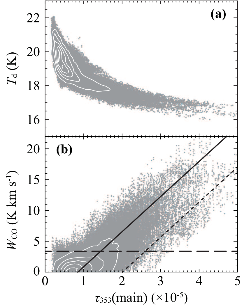
Figure 5: (a) Correlation plot between $T_{\mathrm{d}}$ and $\tau_{353}(\mathrm{main})$ in the area shown in Figure 7(c). The contours represent the $90\,\%$, $70\,\%$, $50\,\%$, $30\,\%$, and $10\,\%$ levels of the maximum of the density of the plotted data over the ($T_{\mathrm{d}}$, $\tau_{353}(\mathrm{main})$) space. (b) same as (a) but for $W_{\mbox{\scriptsize CO}}$ and $\tau_{353}(\mathrm{main})$. The contours represent the $90\,\%$, $70\,\%$, $50\,\%$, $30\,\%$, and $10\,\%$ levels of the maximum of the density of the plotted data over the ($W_{\mbox{\scriptsize CO}}$, $\tau_{353}(\mathrm{main})$) space. The dashed line represents $3\,\sigma$ level of the CO data ($3.4\,\mathrm{K\,km\,s^{-1}}$), and the solid line a relationship $\tau_{353}(\mathrm{main})=[(1.8\pm 0.8)\times 10^{-6}]\cdot W_{\mbox{\scriptsize CO}}\,(\mathrm{K\,km\,s^{-1}})+[(8.4\pm 5.0)\times 10^{-6}]$, which is the result of a least-squares fit to the data with $W_{\mbox{\scriptsize CO}}>3\,\sigma$. The dotted line is $\tau_{353}(\mathrm{main})=(1.8\times 10^{-6})\cdot W_{\mbox{\scriptsize CO}}\,(\mathrm{K\,km\,s^{-1}})+(2\times 10^{-5})$ (see text).

Figure 5(a) shows a scatter plot of $T_{\mathrm{d}}$ and $\tau_{353}(\mathrm{main})$, and clearly indicates a significant decrease of $T_{\mathrm{d}}$ with $\tau_{353}(\mathrm{main})$. A similar result that the dust temperature increases with decreasing gas column density has recently been found by the Planck Collaboration (Planck Collaboration et al., 2014, 2014). Figure 5(b) shows a scatter plot of $W_{\mbox{\scriptsize CO}}$ and $\tau_{353}(\mathrm{main})$ in the area observed in CO. This shows positive correlation with a correlation coefficient of ${\sim}0.7$, while the dispersion is large. The solid line in (b) represents a relationship $\tau_{353}(\mathrm{main})=[(1.8\pm 0.8)\times 10^{-6}]\cdot W_{\mbox{\scriptsize CO}}\,(\mathrm{K\,km\,s^{-1}})+[(8.4\pm 5.0)\times 10^{-6}]$, which is the result of a least-squares fit to the data with $W_{\mbox{\scriptsize CO}}\geq 3\,\sigma$.

4 Analysis

From the behavior in Figure 3 we infer that for the highest $T_{\mathrm{d}}$ the optically thin approximation of H I is valid, whereas for lower $T_{\mathrm{d}}$ the approximation becomes worse due to large H I optical depth. Equation (1) is used to estimate $N_{\mbox{{\scriptsize H}{\tiny\,I}}}$ for the optically thin part in Figure 3,

$$N_{\mbox{{\scriptsize H}{\tiny\,I}}}\,(\mathrm{cm^{-2}})=(1.823\times 10^{18})\allowbreak\cdot W_{\mbox{{\scriptsize H}{\tiny\,I}}}\,(\mathrm{K\,km\,s^{-1}}),$$ (1)

and the relationship between $\tau_{353}(\mathrm{main})$ and $N_{\mbox{{\scriptsize H}{\tiny\,I}}}(\mathrm{main})$ is estimated for the optically thin regime at $T_{\mathrm{d}}\geq 21.5\,\mathrm{K}$;

$$N_{\mbox{{\scriptsize H}{\tiny\,I}}}(\mathrm{main})\,(\mathrm{cm^{-2}})=(1.5\times 10^{26})\cdot\tau_{353}(\mathrm{main}),$$ (2)

where $1.5\times 10^{26}$ is calculated by a product of $1.823\times 10^{18}$ in equation (1) and the slope $k$ ($=8.47\times 10^{7}\,\mathrm{K\,km\,s^{-1}}$) for $T_{\mathrm{d}}>21.5\,\mathrm{K}$ in Table 2.

Relation (2) holds as long as the dust properties are uniform, allowing us to calculate $N_{\mbox{{\scriptsize H}{\tiny\,I}}}(\mathrm{main})$ from $\tau_{353}(\mathrm{main})$. Then the coupled equations (3) and (4) in the following are used to solve for $T_{\mathrm{s}}$ and $\tau_{\mbox{{\scriptsize H}{\tiny\,I}}}(\mathrm{main})$, where $N_{\mbox{{\scriptsize H}{\tiny\,I}}}(\mathrm{main})$ is calculated from $\tau_{353}(\mathrm{main})$ by equation (2),

$$W_{\mbox{{\scriptsize H}{\tiny\,I}}}(\mathrm{main})\,(\mathrm{K\,km\,s^{-1}}) = [T_{\mathrm{s}}\,(\mathrm{K})-T_{\mathrm{bg}}\,(\mathrm{K})]\allowbreak\cdot\mathit{\Delta}V_{\mbox{{\scriptsize H}{\tiny\,I}}}\,(\mathrm{km\,s^{-1}})\cdot\left[1-\rm{exp}(-\tau_{\mbox{{\scriptsize H}{\tiny\,I}}}(\mathrm{main}))\right],$$ (3)

$$\tau_{\mbox{{\scriptsize H}{\tiny\,I}}}(\mathrm{main}) = \frac{N_{\mbox{{\scriptsize H}{\tiny\,I}}}(\mathrm{main})\,(\mathrm{cm^{-2}})}{1.823\times 10^{18}}\cdot\frac{1}{T_{\mathrm{s}}\,(\mathrm{K})}\cdot\frac{1}{\mathit{\Delta}V_{\mbox{{\scriptsize H}{\tiny\,I}}}\,(\mathrm{km\,s^{-1}})},$$ (4)

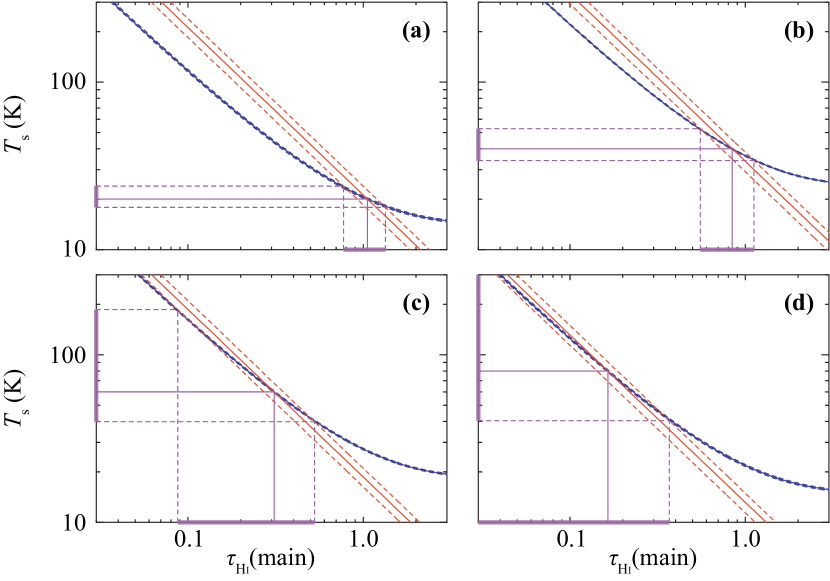
Figure 6: The blue and red lines represent equations (3) and (4) in the text, respectively. The crossing point of the two lines is the solution that satisfies both equations (3) and (4). (a), (b), (c), and (d) show the typical cases of the solutions of $T_{\mathrm{s}}\simeq 20\,\mathrm{K}$, $\simeq 40\,\mathrm{K}$, $\simeq 60\,\mathrm{K}$, and $\simeq 80\,\mathrm{K}$, and are located at $(\ell,b)\sim(92\fdg 70,-41\fdg 56)$, $(90\fdg 07,-42\fdg 68)$, $(89\fdg 69,-29\fdg 12)$, and $(86\fdg 03,-30\fdg 09)$, respectively. The dashed lines around each line are the error taking observational parameters into consideration. The purple solid lines indicate the solutions of $\tau_{\mbox{{\scriptsize H}{\tiny\,I}}}(\mathrm{main})$ and $T_{\mathrm{s}}$, and dashed lines their errors.

where $\mathit{\Delta}V_{\mbox{{\scriptsize H}{\tiny\,I}}}$, the H I linewidth, is given by $W_{\mbox{{\scriptsize H}{\tiny\,I}}}(\mathrm{main})/(\mathrm{peak\ \mbox{H\footnotesize\,I}\ brightness\ temperature})$, and $T_{\mathrm{bg}}$ is the background continuum radiation temperature (see Section 2.4.) including the $2.7\,\mathrm{K}$ cosmic background radiation (Fixsen, 2009). $\tau_{\mbox{{\scriptsize H}{\tiny\,I}}}(\mathrm{main})$ is the H I optical depth averaged over the H I velocity width $\mathit{\Delta}V_{\mbox{{\scriptsize H}{\tiny\,I}}}$, which ranges from $8\,\mathrm{km\,s^{-1}}$ to $30\,\mathrm{km\,s^{-1}}$ with a median at $\sim 14\,\mathrm{km\,s^{-1}}$. Note that equation (4) is valid not only for small $\tau_{\mbox{{\scriptsize H}{\tiny\,I}}}$ but also for any positive value of $\tau_{\mbox{{\scriptsize H}{\tiny\,I}}}$. Figure 6 shows the two relationships in the $T_{\mathrm{s}}\mbox{-}\tau_{\mbox{{\scriptsize H}{\tiny\,I}}}(\mathrm{main})$ plane for four typical values of $T_{\mathrm{s}}\simeq 20\,\mathrm{K}$ (a), $40\,\mathrm{K}$ (b), $60\,\mathrm{K}$ (c), and $80\,\mathrm{K}$ (d). We estimate the errors in $T_{\mathrm{s}}$ as shown in Figure 6 from the $1\,\sigma$ noise level of the H I and $\tau_{353}(\mathrm{main})$ data. We find that the equations give reasonable solutions with small errors for lower $T_{\mathrm{s}}$, whereas they cannot give a single set of $T_{\mathrm{s}}$ and $\tau_{\mbox{{\scriptsize H}{\tiny\,I}}}(\mathrm{main})$ for $T_{\mathrm{s}}$ higher than $\sim 70\,\mathrm{K}$, where the error bars in $T_{\mathrm{s}}$ become uncomfortably large. In Figure 6, we estimate the error ranges as follows: (a) $T_{\mathrm{s}}\simeq 20^{+4}_{-2}\,\mathrm{K}$, $\tau_{\mbox{{\scriptsize H}{\tiny\,I}}}(\mathrm{main})\simeq 1.06^{+0.28}_{-0.29}$, (b) $T_{\mathrm{s}}\simeq 40^{+13}_{-6}\,\mathrm{K}$, $\tau_{\mbox{{\scriptsize H}{\tiny\,I}}}(\mathrm{main})\simeq 0.84^{+0.28}_{-0.29}$, (c) $T_{\mathrm{s}}\simeq 60^{+126}_{-20}\,\mathrm{K}$, $\tau_{\mbox{{\scriptsize H}{\tiny\,I}}}(\mathrm{main})\simeq 0.31^{+0.21}_{-0.22}$, and (d) $T_{\mathrm{s}}\simeq 80^{+\infty}_{-39}\,\mathrm{K}$, $\tau_{\mbox{{\scriptsize H}{\tiny\,I}}}(\mathrm{main})\simeq 0.16^{+0.20}_{-0.16}$. In the optically thin limit, the two equations become essentially the same, and can be satisfied by an infinite number of solutions, either a combination of large $T_{\mathrm{s}}$ and small $\tau_{\mbox{{\scriptsize H}{\tiny\,I}}}(\mathrm{main})$, or that of small $T_{\mathrm{s}}$ and large $\tau_{\mbox{{\scriptsize H}{\tiny\,I}}}(\mathrm{main})$. Only the lower limit for $T_{\mathrm{s}}$ and the upper limit of $\tau_{\mbox{{\scriptsize H}{\tiny\,I}}}(\mathrm{main})$ are constrained.

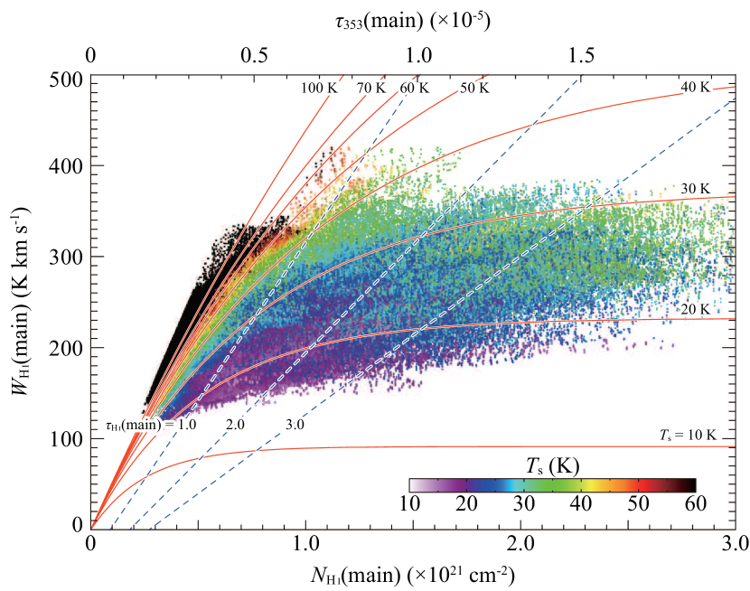
Figure 8: Correlation plot between $W_{\mbox{{\scriptsize H}{\tiny\,I}}}(\mathrm{main})$ and $N_{\mbox{{\scriptsize H}{\tiny\,I}}}(\mathrm{main})$. The data in the region shown in the Figure 7(a)(b) is plotted. The color of each point represents $T_{\mathrm{s}}$. The solid and dashed lines represent $T_{\mathrm{s}}$ and $\tau_{\mbox{{\scriptsize H}{\tiny\,I}}}(\mathrm{main})$ calculated from equations (3) and (4) in the text by assuming $\mathit{\Delta}V_{\mbox{{\scriptsize H}{\tiny\,I}}}$ of $\sim 14.1\,\mathrm{km\,s^{-1}}$ (median value) and $T_{\mathrm{bg}}$ of $\sim 3.5\,\mathrm{K}$ (median value), respectively.

Figure 7(a) shows the distribution of $T_{\mathrm{s}}$, Figure 7(b) the distribution for $\tau_{\mbox{{\scriptsize H}{\tiny\,I}}}(\mathrm{main})$, and Figure 7(c) the distribution of $\tau_{353}(\mathrm{main})$. Several specific areas are masked as described in Section 3 and also masked where the estimated $T_{\mathrm{s}}$ is greater than $70\,\mathrm{K}$. In Figure 7(a) $T_{\mathrm{s}}$ is mostly lower than $50\,\mathrm{K}$. We also find that $\tau_{\mbox{{\scriptsize H}{\tiny\,I}}}(\mathrm{main})$ becomes large in many of the data points. The results for $T_{\mathrm{s}}$ and $\tau_{\mbox{{\scriptsize H}{\tiny\,I}}}(\mathrm{main})$ estimated are plotted in Figure 8 with superposition of equation (3) for $T_{\mathrm{s}}$ from $10\,\mathrm{K}$ to $100\,\mathrm{K}$ with $\tau_{\mbox{{\scriptsize H}{\tiny\,I}}}(\mathrm{main})$. We see saturation of $W_{\mbox{{\scriptsize H}{\tiny\,I}}}(\mathrm{main})$ becomes important for lower $T_{\mathrm{s}}$, and the slope for a given $T_{\mathrm{s}}$ decreases with decreasing $T_{\mathrm{s}}$ due to saturation. This result is consistent with $T_{\mathrm{s}}$ estimated from comparisons between H I emission and absorption toward radio continuum sources, which show that cold H I clouds of $20\,\mathrm{K}\mbox{--}40\,\mathrm{K}$ are common (Dickey et al., 2003; Heiles & Troland, 2003). Their spatial coverage is however much smaller than the present coverage, $100\,\mathrm{square\mbox{-}degrees}$. Possible hints of optically thick H I are also found in the literature (Strasser & Taylor, 2004; Dickey, 2010).

5 Physical conditions in the H I gas

5.1 $T_{\mathrm{d}}$ and $T_{\mathrm{s}}$

The present analysis offers evidence for a significant fraction of cold H I gas in the region. The analysis shows the typical physical parameters of the optically thick H I gas as follows: $N_{\mbox{{\scriptsize H}{\tiny\,I}}}(\mathrm{main})=4\times 10^{20}\,\mathrm{cm^{-2}}\mbox{--}1.5\times 10^{21}\,\mathrm{cm^{-2}}$, H I number density $n_{\mbox{{\scriptsize H}{\tiny\,I}}}=40\,\mathrm{cm^{-3}}\mbox{--}160\,\mathrm{cm^{-3}}$ for cloud line-of-sight depth of $3\,\mathrm{pc}$, and $T_{\mathrm{s}}=20\,\mathrm{K}\mbox{--}40\,\mathrm{K}$. The gas kinetic temperature of the H I is determined by heating due to the interstellar radiation field (ISRF) and cooling mainly by the C II line (e.g., Wolfire et al., 1995) and is in a range from $10\,\mathrm{K}\mbox{--}100\,\mathrm{K}$ for column density higher than $2\times 10^{20}\,\mathrm{cm^{-2}}$ (e.g., Goldsmith et al., 2007). Since the radiative transition rate, the Einstein $A$ coefficient, of the $21\,\mathrm{cm}$ line is small, $\sim 3\times 10^{-15}\,\mathrm{s^{-1}}$, the $21\,\mathrm{cm}$ transition is well thermalized by collisional excitation for density higher than ${\sim}10\,\mathrm{cm^{-3}}$ (e.g., Liszt, 2001; Sato & Fukui, 1978). $T_{\mathrm{s}}$ is exactly in equilibrium with the gas kinetic temperature in the dense H I gas. On the other hand, $T_{\mathrm{d}}$ is determined by the balance between the ISRF heating and thermal radiation of dust grains and is generally in a range from $15\,\mathrm{K}$ to $25\,\mathrm{K}$ in the H I gas. $T_{\mathrm{d}}$ and $T_{\mathrm{s}}$ should show correlation, since heating is commonly due to the ISRF, where $T_{\mathrm{d}}$ variation is much smaller than that of $T_{\mathrm{s}}$ due to the strong temperature dependence of the dust cooling, as $(T_{\mathrm{d}})^{6}$ (e.g., Draine, 2011). For $A_{V}$ more than $1\,\mathrm{mag}$, $T_{\mathrm{s}}$ becomes less than $60\,\mathrm{K}$ (e.g., Goldsmith et al., 2007), and $T_{\mathrm{d}}$ shows significant decrease to $17\,\mathrm{K}$, which corresponds to $T_{\mathrm{d}}$ within the CO clouds (Figure 1). The present results on $T_{\mathrm{s}}$ and $\tau_{\mbox{{\scriptsize H}{\tiny\,I}}}(\mathrm{main})$ are therefore consistent with the thermal properties of the ISM. It is possible that $T_{\mathrm{d}}$ is affected by the local radiation field in addition to the general ISRF. The distribution of $T_{\mathrm{d}}$ shown in Figure 1(c) indicates that in the northwest of the CO clouds $T_{\mathrm{d}}$ tends to be higher than in the southeast. This may be due to the excess radiation field of the OB stars in the Sco OB2 association which are located $100\mbox{--}200\,\mathrm{pc}$ away from the present clouds (c.f., Tachihara et al., 2001).

An $X_{\mbox{\scriptsize CO}}$ factor converting $W_{\mbox{\scriptsize CO}}$ into $N_{\mbox{{\scriptsize H}}_{2}}$ is estimated from a comparison of CO and $\tau_{353}(\mathrm{main})$ (Figure 5(b)). A least-squares fit for $W_{\mbox{\scriptsize CO}}$ greater than $3.4\,\mathrm{K\,km\,s^{-1}}$ (above the $3\,\sigma$ noise level) yields $\tau_{353}(\mathrm{main})=[(1.8\pm 0.8)\times 10^{-6}]\cdot W_{\mbox{\scriptsize CO}}\,(\mathrm{K\,km\,s^{-1}})+[(8.4\pm 5.0)\times 10^{-6}]$. Here we adopt $W_{\mbox{\scriptsize CO}}$ greater than $3\,\sigma$ by considering that an $X_{\mbox{\scriptsize CO}}$ factor is conventionally estimated for $A_{V}\gtrsim 2\mbox{--}3\,\mathrm{mag}$ (e.g. Bell et al., 2006). The offset $8.4\times 10^{-6}$ in $\tau_{353}(\mathrm{main})$ in the above relationship is interpolated as due to the contribution of the H I, and the $X_{\mbox{\scriptsize CO}}$ factor is calculated from the slope $1.8\times 10^{-6}$ in the relationship and the coefficient in equation (2) as $X_{\mbox{\scriptsize CO}}=N_{\mbox{{\scriptsize H}}_{2}}/W_{\mbox{\scriptsize CO}}=(1.5\times 10^{26}/2)\cdot(1.8\times 10^{-6})=1.3\times 10^{20}\,\mathrm{cm^{-2}/(K\,km\,s^{-1})}$ with typical dispersion of $\sim\pm 40\,\%$, which is somewhat smaller than that estimated elsewhere, $(2\mbox{--}3)\times 10^{20}\,\mathrm{cm^{-2}/(K\,km\,s^{-1})}$ (e.g., Bertsch et al., 1993). Numerical simulations suggest that the $X_{\mbox{\scriptsize CO}}$ factor is relatively uniform in regions of high visual extinction where CO is intense (Inoue & Inutsuka, 2012; Glover & Mac Low, 2011; Bell et al., 2006). This difference may be possibly ascribed to the large contribution of cold H I gas which was not taken into account previously, and should be confirmed by a careful analysis of more sample clouds. We note that we see a small number of points in Figure 5(b) which show higher $\tau_{353}(\mathrm{main})$ for a given $W_{\mbox{\scriptsize CO}}$ on the right of the dotted line and above the dashed line. These may correspond to the molecular gas with slightly less CO abundance than the majority, suggesting a younger chemical evolutionary stage (Yamamoto et al., 2003), and can be characterized by a higher $X_{\mbox{\scriptsize CO}}$ factor.

5.2 Alternative ideas

The above interpretation assumes that all the neutral gas outside the CO is purely atomic. This interpretation is consistent with the present analysis including only H I as shown by the fit of the line radiation transfer equation and estimated $T_{\mathrm{s}}$ and $\tau_{\mbox{{\scriptsize H}{\tiny\,I}}}(\mathrm{main})$ (Figure 7). We shall test if an interpretation based on CO-free $\mbox{H}_{2}$ is possible as an alternative, which was advocated for a giant molecular cloud having total mass of $10^{5}\,M_{\odot}\mbox{--}10^{6}\,M_{\odot}$ by Wolfire et al. (2010) and was discussed in the first Planck paper (Planck Collaboration et al., 2011b). $\tau_{353}(\mathrm{main})$ is a sum of the dust opacity both in the H I and $\mbox{H}_{2}$ gas. If CO-free $\mbox{H}_{2}$ is dominant, $\mbox{H}_{2}$ may account for most of the $\tau_{353}(\mathrm{main})$ instead of H I. The observed value of $W_{\mbox{{\scriptsize H}{\tiny\,I}}}(\mathrm{main})$ poses a strict lower limit on $N_{\mbox{{\scriptsize H}{\tiny\,I}}}(\mathrm{main})$ and it is not probable that $\mbox{H}_{2}$ dominates H I. The majority of the data points have $T_{\mathrm{s}}\sim 30\,\mathrm{K}$ (Figure 8) and a lower limit for their H I column density is given by the optically thin limit. For instance, for points having $W_{\mbox{{\scriptsize H}{\tiny\,I}}}(\mathrm{main})=250\,\mathrm{K\,km\,s^{-1}}$, $N_{\mbox{{\scriptsize H}{\tiny\,I}}}(\mathrm{main})$ at $T_{\mathrm{s}}\sim 30\,\mathrm{K}$ is $0.85\times 10^{21}\,\,\mathrm{cm^{-2}}$, whereas $N_{\mbox{{\scriptsize H}{\tiny\,I}}}(\mathrm{main})$ in the optically thin limit is $0.45\times 10^{21}\,\mathrm{cm^{-2}}$ corresponding to ${\sim}50\,\%$ of $0.85\times 10^{21}\,\,\mathrm{cm^{-2}}$, and for points having $W_{\mbox{{\scriptsize H}{\tiny\,I}}}(\mathrm{main})=200\,\mathrm{K\,km\,s^{-1}}$, $N_{\mbox{{\scriptsize H}{\tiny\,I}}}(\mathrm{main})$ at $T_{\mathrm{s}}\sim 30\,\mathrm{K}$ is $0.6\times 10^{21}\,\mathrm{cm^{-2}}$ whereas $N_{\mbox{{\scriptsize H}{\tiny\,I}}}(\mathrm{main})$ in the optically thin limit is $0.35\times 10^{21}\,\mathrm{cm^{-2}}$ corresponding to ${\sim}60\,\%$ of $0.6\times 10^{21}\,\,\mathrm{cm^{-2}}$. This suggests that the cold gas typically has $\mbox{H}_{2}$ abundance of $50\,\%$ or less over most of the region outside of the CO clouds. Direct UV absorption measurements of $\mbox{H}_{2}$ abundances on the line of sight toward NGC 7469 ($\ell=83\fdg 10,b=-45\fdg 47$) show $N_{\mbox{{\scriptsize H}}_{2}}=4.7\times 10^{19}\,\mathrm{cm^{-2}}$ and $N_{\mbox{{\scriptsize H}{\tiny\,I}}}=3.9\times 10^{20}\,\mathrm{cm^{-2}}$ (Gillmon et al., 2006), indicating that the hydrogen is about $90\,\%$ atomic. It is worth noting that other lines of sight at intermediate latitudes observed by FUSE and Copernicus (summarized by Rachford et al., 2009) show similarly low molecular fractions unless the total H column density, $N_{\mbox{{\scriptsize H}}_{2}}+N_{\mbox{{\scriptsize H}{\tiny\,I}}}\gtrsim 10^{21}\,\mathrm{cm^{-2}}$, lending support for the conclusion that H I is dominant. Finally, we note that the timescale for $\mbox{H}_{2}$ formation is generally as long as $10^{7}\,\mathrm{years}$ for typical density $100\,\mathrm{cm^{-3}}$ (Hollenbach et al., 1971). The cloud lifetime is however smaller than $\sim 10^{6}\,\mathrm{years}$ as estimated from the crossing time at latitude higher than $10\,\mathrm{degrees}$ for a typical cloud size of several $\mathrm{pc}$ and a line width of $15\,\mathrm{km\,s^{-1}}$ (Yamamoto et al., 2003, 2006). This suggests that the present cloud is too young to form significant $\mbox{H}_{2}$. Another possibility is that the dust properties may be considerably different in the region, as has been explored by the Planck collaboration (Planck Collaboration et al., 2014). We shall defer exploration of this possibility until a full account of the study is opened to the community.

5.3 Mass of the H I envelope

We estimate the total mass of the clouds in the region under study. We estimate the total system mass including H I, $\mbox{H}_{2}$, and $\mathrm{He}$ ($40\,\%$ of hydrogen in mass) to be $\sim 1.3\times 10^{4}\,M_{\odot}$, by using the sum of $\tau_{353}(\mathrm{main})$ above $5\times 10^{-6}$ under equation (2) applied both to H I and $\mbox{H}_{2}$ (Figure 7(c)). The typical ratio of the opacity-corrected case to the optically thin case is estimated to be $\sim 2.7$ toward areas without CO emission, showing that the opacity correction has a significant impact. The mass of the H I gas in the masked areas is interpolated to be $\sim 9.0\times 10^{2}\,M_{\odot}$ by using the average $N_{\mbox{{\scriptsize H}{\tiny\,I}}}(\mathrm{main})\sim 1.3\times 10^{21}\,\mathrm{cm^{-2}}$ in the areas without masking, and corresponds to $\sim 7\,\%$ of the total system mass above. On the other hand, the molecular mass is estimated to be $\sim 1.2\times 10^{3}\,M_{\odot}$ by applying the present $X_{\mbox{\scriptsize CO}}$ factor ($=1.3\times 10^{20}\,\mathrm{cm^{-2}/(K\,km\,s^{-1})}$) to the CO emission. Here we integrated the CO emission above the $3\,\sigma$ noise fluctuations of $3.4\,\mathrm{K\,km\,s^{-1}}$ in the integrated intensity in the $5\,\mathrm{arcmin}$ smoothed beam. By subtracting this mass from the total system mass, we obtain $\sim 1.2\times 10^{4}\,M_{\odot}$ as the total mass of the H I envelope. We thus find that the H I envelope has a total mass $\sim 10$ times larger than the mass of the $\mbox{H}_{2}$ clouds probed by CO. Note that in Gir et al. (1994) the mass of the H I envelope was calculated as $\sim 3\times 10^{3}\,M_{\odot}$, which is smaller than the present result. This difference may be attributed to the fact that (i) the area they used for the calculation corresponds to ${\sim}1/2$ of that used in our calculation, and (ii) they assumed that all the H I gas is optically thin.

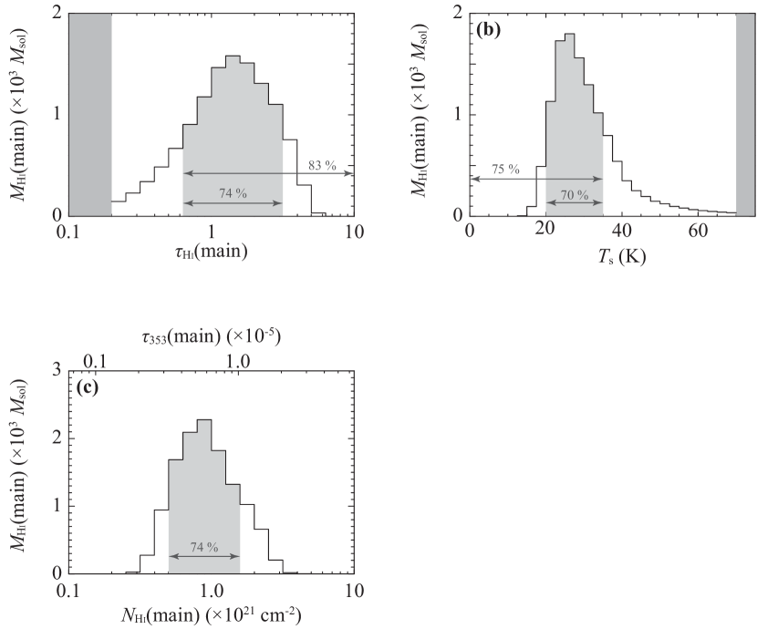
Figure 9: (a) Histogram of the mass of the H I envelope as a function of $\tau_{\mbox{{\scriptsize H}{\tiny\,I}}}(\mathrm{main})$. (b) The same as (a), but as a function of $T_{\mathrm{s}}$. (c) The same as (a) and (b), but as functions of $N_{\mbox{{\scriptsize H}{\tiny\,I}}}(\mathrm{main})$ and $\tau_{353}(\mathrm{main})$. The areas filled with light-gray are determined by the widths at the half-levels of the each histogram. Note that in panels (a) and (b), the histograms where $\tau_{\mbox{{\scriptsize H}{\tiny\,I}}}(\mathrm{main})\leq 0.2$ or $T_{\mathrm{s}}\geq 70\,\mathrm{K}$ are masked because the solutions of $\tau_{\mbox{{\scriptsize H}{\tiny\,I}}}(\mathrm{main})$ and $T_{\mathrm{s}}$ are not well-estimated.

We conclude that the $\mbox{H}_{2}$ clouds traced by CO are surrounded by massive, optically thick H I envelopes possibly containing a relatively small fraction of $\mbox{H}_{2}$ that has no corresponding CO emission above the $3\,\sigma$ noise fluctuations of $3.4\,\mathrm{K\,km\,s^{-1}}$. Figure 9 is a histogram of the mass of the H I envelope as a function of $T_{\mathrm{s}}$. This clearly shows that most of the H I is in the $T_{\mathrm{s}}$ ranges from $20\,\mathrm{K}$ to $40\,\mathrm{K}$. Assuming the depth of the H I envelope along the line of sight to be $3\,\mathrm{pc}$, the H I density is estimated to be $40\,\mathrm{cm^{-3}}\mbox{--}160\,\mathrm{cm^{-3}}$. This density is consistent with $T_{\mathrm{s}}=20\,\mathrm{K}\mbox{--}40\,\mathrm{K}$ in a model calculation of the thermal balance (Goldsmith et al., 2007).

It is generally known that small clouds having mass less than $\sim 1000\,M_{\odot}$ cannot be gravitationally bound due to the large virial mass as compared with the CO luminosity mass (e.g., Yonekura et al., 1997; Kawamura et al., 1998). The H I envelope may have a deep influence on cloud dynamics. The average density of the H I is $100\,\mathrm{cm^{-3}}$ and the velocity width is $15\,\mathrm{km\,s^{-1}}$. The dynamical pressure of H I, $\rho\,v^{2}$ $[(\mathrm{density})\cdot(\mathrm{velocity\ dispersion})^{2}]$, is nearly equal to that of the $\mbox{H}_{2}$ gas and the pressure exerted by the H I envelope is able to confine the $\mbox{H}_{2}$. The H I envelope may help to stabilize small $\mbox{H}_{2}$ clouds. It is yet perhaps true that the whole system including the H I envelope is not gravitationally bound because of the large velocity dispersion of the H I, and some dynamically transient states, like those in colliding H I flows, must be invoked to explain the cloud dynamics (e.g., Hartmann et al., 2001).

5.4 Relation to the dark gas

Recent analyses of gamma ray maps and the Planck data show evidence for dark gas which is not seen in CO or H I emission (Grenier et al., 2005; Planck Collaboration et al., 2011b). These analyses did not consider the H I opacity effect and assumed that H I is completely optically thin. The present study has shown that the H I optical depth effect is important in this region and an upward correction of the cloud mass by a factor of $\sim 2$ on average is required. A significant fraction of the relatively dense H I gas may therefore be masked by saturation of the $21\,\mathrm{cm}$ line, and the cold H I gas is a viable candidate for the dark gas. This possibility deserves further exploration by including a much larger fraction of the sky. We note that the present analysis is applicable in a $\tau_{353}(\mathrm{main})$ range from $2\times 10^{-6}$ to $\mathrm{a\ few\times 10^{-5}}$. Therefore, the behavior of the H I outside this range is yet to be explored separately.

6 Conclusions

We have made a comparison of H I, CO, and the Planck dust properties in a complex of high latitude clouds MBM 53, 54, 55 (catalog ) and HLCG $92{-}35$ (catalog ) and conclude from this study as follows;

The H I intensity shows a poor correlation with dust opacity with a correlation coefficient of $\sim 0.6$. We interpret that this is caused by the effect of the optical depth on $21\,\mathrm{cm}$ H I emission. We present a method to estimate the spin temperature and the optical depth of the H I emission which couples the equation of line radiation transfer and the expression for the H I optical depth by assuming that dust properties do not change significantly in the region, where the $\tau_{353}(\mathrm{main})$ is limited in a range from $3\times 10^{-6}$ to $2\times 10^{-5}$. We have analyzed about $8\times 10^{5}$ data points smoothed at $5\,\mathrm{arcmin}$ resolution and successfully estimated $T_{\mathrm{s}}$ and $\tau_{\mbox{{\scriptsize H}{\tiny\,I}}}(\mathrm{main})$. Most of the points have $T_{\mathrm{s}}$ in the range from $20\,\mathrm{K}$ to $40\,\mathrm{K}$ and $\tau_{\mbox{{\scriptsize H}{\tiny\,I}}}(\mathrm{main})$ is in the range from $0.2$ to $4$. This indicates that saturation due to large H I optical depth provides a reasonable explanation of the suppressed H I intensity in regions with large dust opacity. The $T_{\mathrm{s}}$ distribution is consistent with previous results estimated from absorption measurements toward radio continuum sources while in this paper the spatial coverage is continuous, covering a much larger area than continuum source absorption measurements. If the present results are correct, this suggests that optically thick H I is more significant than previously assumed in the literature. The typical physical parameters of the cold H I are density $40\,\mathrm{cm^{-3}}\mbox{--}160\,\mathrm{cm^{-3}}$, $T_{\mathrm{s}}=20\,\mathrm{K}\mbox{--}40\,\mathrm{K}$ and $N_{\mbox{{\scriptsize H}{\tiny\,I}}}(\mathrm{main})=4\times 10^{20}\,\mathrm{cm^{-2}}\mbox{--}1.5\times 10^{21}\,\mathrm{cm^{-2}}$. The $X_{\mbox{\scriptsize CO}}$ factor to covert $W_{\mbox{\scriptsize CO}}$ into $N_{\mbox{{\scriptsize H}}_{2}}$ has been estimated to be $1.3\times 10^{20}\,\mathrm{cm^{-2}/(K\,km\,s^{-1})}$. The CO clouds are associated with massive dense cold H I envelope having $\sim 1.2\times 10^{4}\,M_{\odot}$ as compared with the CO cloud mass of $\sim 1.2\times 10^{3}\,M_{\odot}$. Another possibility, that the dust properties may vary significantly, is being explored currently by the Planck collaboration, and should be considered in depth as a future step. Finally, it is an obvious task to extend this method to the whole sky to see if cold H I is common and dominant in the local interstellar space around the Sun.

Appendix A

Figure 10 shows five H I velocity channel distributions from $V_{\mathrm{LSR}}=-45\,\mathrm{km\,s^{-1}}$ to $+32\,\mathrm{km\,s^{-1}}$. The main H I cloud toward the CO emitting clouds is seen from $-12.7\,\mathrm{km\,s^{-1}}$ to $-0.3\,\mathrm{km\,s^{-1}}$ (panel (b)) as noted by Gir et al. (1994). The main feature is outstanding in the H I intensity having $200\,\mathrm{K\,km\,s^{-1}}$ in the integrated intensity. In this velocity channel, we see additional H I features; one is located $\sim 5\,\mathrm{degree}$ west of the main cloud and is elongated in a similar direction and with similar length to the main cloud (called West1 H I), and the other in the north of the main cloud peaked at $(l,b)\sim(100^{\circ},-31^{\circ})$ (North H I). West1 H I seems to be linked with the northern tip of the CO clouds. We also find an additional feature (West2 H I) peaked at $(l,b)\sim(90^{\circ},-37^{\circ})$ which may be extended to the west up to $l\sim 80^{\circ}$.

In $V_{\mathrm{LSR}}$ from $-25.0\,\mathrm{km\,s^{-1}}$ to $-12.7\,\mathrm{km\,s^{-1}}$ (panel (a)), we see two features; one of them corresponds to North H I in position and the other to West2 H I. In addition, the H I, North H I and several smaller peaks along the southern rim of the main cloud, seems to be surrounding the CO as noted by Yamamoto et al. (2003) (see also their Figure 6).

In the velocity from $-0.3\,\mathrm{km\,s^{-1}}$ to $+12.0\,\mathrm{km\,s^{-1}}$ (panel (c)), we see the H I corresponds to West1 H I and the H I in the north shows intensity depression surrounding the CO, suggesting physical association with the CO.

In the other extreme velocity range from $-45.0\,\mathrm{km\,s^{-1}}$ to $-25.0\,\mathrm{km\,s^{-1}}$ (panel (d)) we find the main peak at $(l,b)\sim(87^{\circ},-38^{\circ})$ shows elongation similar to West2 H I. The H I may be possibly linked with West2, while it was not included in the present analysis.

We summarize the above that the H I in the three panels (a), (b) and (c) is likely associated with the main cloud within a volume having a size in the order of the main H I cloud, $30\mbox{--}40\,\mathrm{pc}$, at a distance of $150\,\mathrm{pc}$.

Appendix B

$\tau_{353}(\mathrm{main})$, which is the main component of $\tau_{353}$, is calculated as follows;

• First we use slope derived by least-squares fits between $W_{\mbox{{\scriptsize H}{\tiny\,I}}}$ and $\tau_{353}$ by linear regression for $T_{\mathrm{d}}>21.5\,\mathrm{K}$ in Figure 4(b).

• By using the slope derived from (1) $\tau_{353}^{\prime}$ is calculated by $\tau_{353}^{\prime}=\tau_{353}-W_{\mbox{{\scriptsize H}{\tiny\,I}}}\,(V_{\mathrm{LSR}}<{-}25\,\mathrm{km\,s^{-1}},{+}12\,\mathrm{km\,s^{-1}}<V_{\mathrm{LSR}})/(\mathrm{slope})$.

• We estimate new slope again by the same manner as (1) between $W_{\mbox{{\scriptsize H}{\tiny\,I}}}(\mathrm{main})$ and $\tau_{353}^{\prime}$.

• $\tau_{353}^{\prime\prime}$ is calculated by the same manner as (2) but by using $\tau_{353}^{\prime}$ and the slope derived by (3).

• Iterating (3) and (4) until the value of the slope becomes converged.

After 5 iterations the best estimate of the slope $k$ converged to $8.34\times 10^{7}\,\mathrm{K\,km\,s^{-1}}$ with the relative variation less than $10^{-4}$.

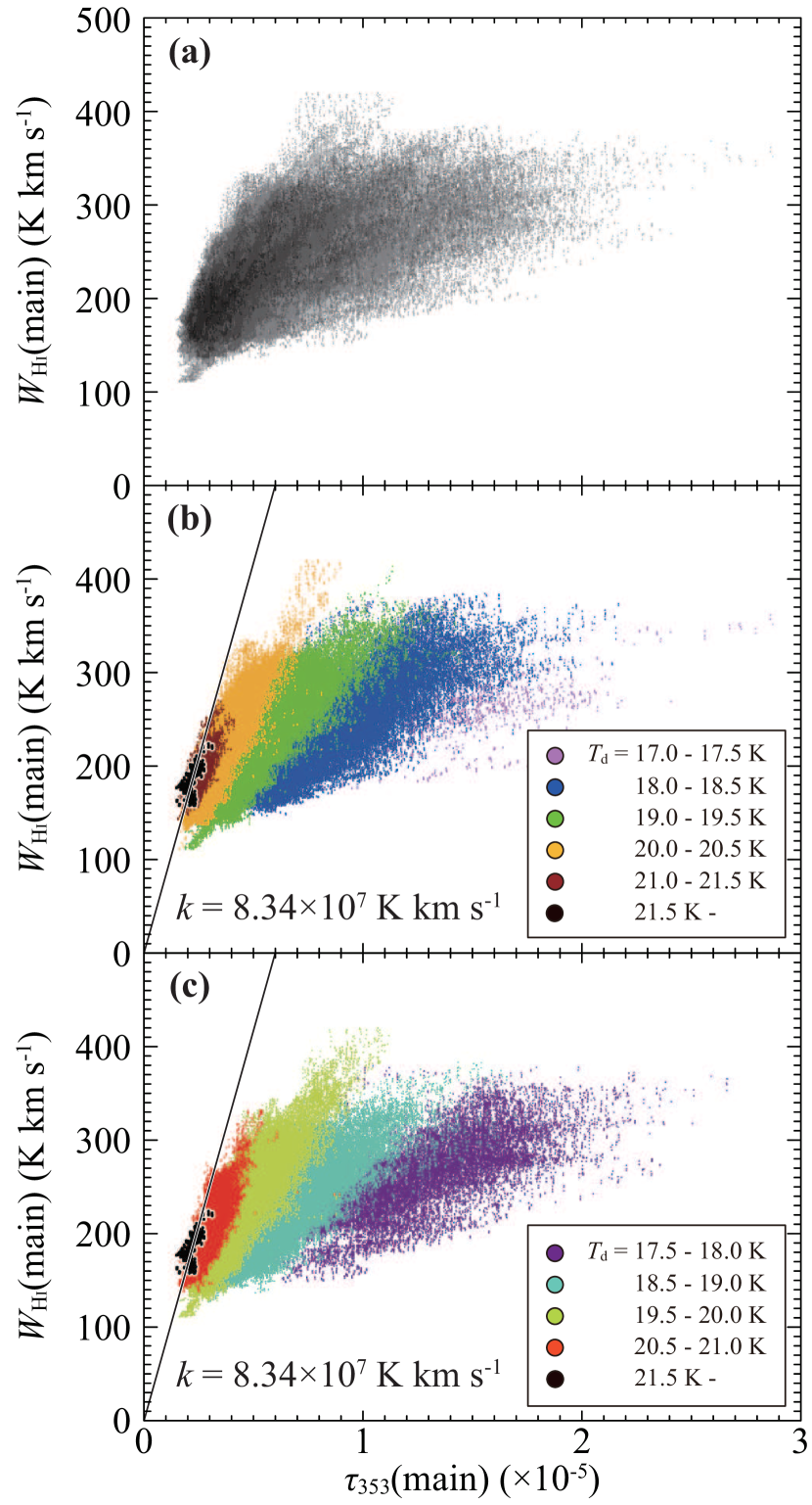
Figure 3: Scatter plots between $W_{\mbox{{\scriptsize H}{\tiny\,I}}}(\mathrm{main})$ and $\tau_{353}(\mathrm{main})$ and between $W_{\mbox{{\scriptsize H}{\tiny\,I}}}$ and $\tau_{353}$ in the region shown in Figure 1. Specific areas are masked. Details on the masking are described in Section 2.5. Figure 3: scatter plots of $W_{\mbox{{\scriptsize H}{\tiny\,I}}}(\mathrm{main})$ whose integrated velocity range is from ${-}25\,\mathrm{km\,s^{-1}}$ to ${+}12\,\mathrm{km\,s^{-1}}$ and $\tau_{353}(\mathrm{main})$, which is the $\tau_{353}$ component associated with the H I whose velocity range is from ${-}25\,\mathrm{km\,s^{-1}}$ to ${+}12\,\mathrm{km\,s^{-1}}$. Details on how to calculate this $\tau_{353}(\mathrm{main})$ value are described in the Appendix B. (a) plots in black dots for all points. (b) and (c) show the scatter plots for $T_{\mathrm{d}}$ in windows of $0.5\,\mathrm{K}$ interval every $1\,\mathrm{K}$. In order to avoid heavy overlapping among the data points, in (b) we show five $T_{\mathrm{d}}$ ranges, $17.0\,\mathrm{K}\mbox{--}17.5\,\mathrm{K}$ (light purple), $18.0\,\mathrm{K}\mbox{--}18.5\,\mathrm{K}$ (blue), $19.0\,\mathrm{K}\mbox{--}19.5\,\mathrm{K}$ (green), $20.0\,\mathrm{K}\mbox{--}20.5\,\mathrm{K}$ (yellow), and $21.0\,\mathrm{K}\mbox{--}21.5\,\mathrm{K}$ (brown), and in (c) five $T_{\mathrm{d}}$ ranges shifted by $0.5\,\mathrm{K}$, $17.5\,\mathrm{K}\mbox{--}18.0\,\mathrm{K}$ (purple), $18.5\,\mathrm{K}\mbox{--}19.0\,\mathrm{K}$ (light blue), $19.5\,\mathrm{K}\mbox{--}20.0\,\mathrm{K}$ (light green), and $20.5\,\mathrm{K}\mbox{--}21.0\,\mathrm{K}$ (red). In the both panels (b) and (c) the $T_{\mathrm{d}}$ range, $21.5\,\mathrm{K}$ and higher, is shown in black along with the linear regression line obtained by the least-squares fit which is assumed to have zero intercept. Figure 4: same as Figure 3 but integrated velocity range of the H I is from ${-}49\,\mathrm{km\,s^{-1}}$ to ${+}17\,\mathrm{km\,s^{-1}}$ and $\tau_{353}$ is the total value.

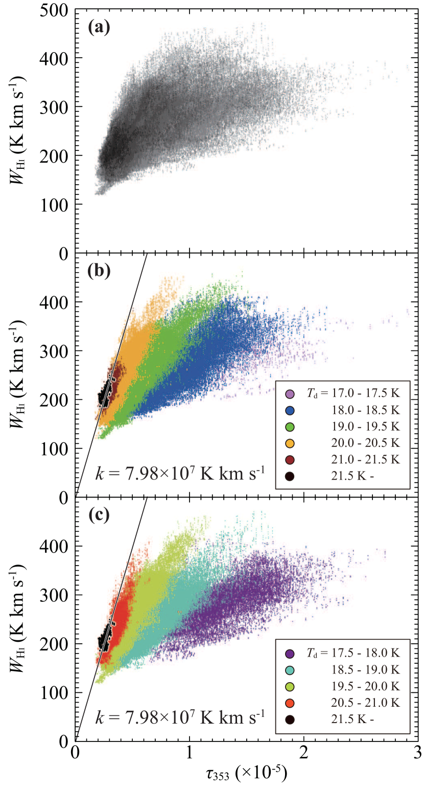
Figure 4:

Table 1: List of masked areas

position		Area	stringObject namestring	stringRemarkstring
$\ell\,(\mathrm{degree})$	$b\,(\mathrm{degree})$	$(\mathrm{degree^{2}})$
$79.1\phantom{0}$	$-41.8\phantom{0}$	$\phantom{0}1.1$	$\cdots$	$(a)$
$81.5\phantom{0}$	$-29.3\phantom{0}$	$\phantom{0}6.5$	$\cdots$	$(a)$
$81.5\phantom{0}$	$-33.0\phantom{0}$	$\phantom{0}6.0$	$\cdots$	$(b)$
$85.6\phantom{0}$	$-33.8\phantom{0}$	$\phantom{0}6.4$	$\cdots$	$(b)$
$86.1\phantom{0}$	$-38.2\phantom{0}$	$13.1$	3C 454.3	$(c)$
$92.2\phantom{0}$	$-38.9\phantom{0}$	$\phantom{0}0.3$	$\cdots$	$(a)$
$98.3\phantom{0}$	$-35.1\phantom{0}$	$\phantom{0}1.0$	$\cdots$	$(a)$
$99.1\phantom{0}$	$-41.6\phantom{0}$	$13.1$	$\cdots$	$(a)$
$99.4\phantom{0}$	$-30.1\phantom{0}$	$\phantom{0}0.7$	$\cdots$	$(a)$
$80.58$	$-32.47$	$8.5\times 10^{-2}$	IRAS 22221+1748	infrared source
$82.42$	$-30.16$	$8.5\times 10^{-2}$	33 Peg	double or multiple star
$83.37$	$-32.25$	$8.6\times 10^{-2}$	Mrk 306	galaxy
$83.46$	$-32.39$	$8.6\times 10^{-2}$	HD 213618	star
$84.67$	$-32.34$	$8.7\times 10^{-2}$	HD 214128	star
$84.73$	$-32.31$	$8.7\times 10^{-2}$	NGC 7316	galaxy
$86.05$	$-33.18$	$8.6\times 10^{-2}$	Mrk 308	Seyfert galaxy
$86.09$	$-33.57$	$8.6\times 10^{-2}$	BD+19 4992	star
$87.46$	$-29.73$	$8.6\times 10^{-2}$	NGC 7339	radio galaxy(d)
$93.53$	$-40.35$	$8.7\times 10^{-2}$	RAFGL 3068	variable star
$93.91$	$-40.47$	$8.7\times 10^{-2}$	NGC 7625	interacting galaxies
$97.29$	$-32.52$	$8.6\times 10^{-2}$	IC 5298	Seyfert 2 galaxy
$98.88$	$-36.55$	$8.6\times 10^{-2}$	NGC 7678	active galaxy nucleus
$99.24$	$-35.40$	$8.6\times 10^{-2}$	NGC 7673	emission-line galaxy
$99.32$	$-35.49$	$8.6\times 10^{-2}$	NGC 7677	galaxy in pair of galaxies

Note. — Columns 1 and 2 give the positions of each mask, and column 3 gives their areas. Column 4 indicates object names located at the center of each mask. Remarks on each masked area are listed in column 5. Details on these masked areas are described in Section 2.5.

Table 2: Parameters of the data points in each $T_{\mathrm{d}}$ range

$T_{\mathrm{d}}$	$N_{\mathrm{pixel}}$	Slope $k$	Intercept	C.C.
$(\mathrm{K})$		$(\mathrm{K\,km\,s^{-1}})$	$(\mathrm{K\,km\,s^{-1}})$
$17.0$–$17.5$	$1.48\times 10^{3}$	$6.83\times 10^{6}$	$1.5\phantom{0}\times 10^{2}$	0.62
$17.5$–$18.0$	$2.73\times 10^{4}$	$9.85\times 10^{6}$	$1.4\phantom{0}\times 10^{2}$	0.72
$18.0$–$18.5$	$8.64\times 10^{4}$	$1.41\times 10^{7}$	$1.2\phantom{0}\times 10^{2}$	0.80
$18.5$–$19.0$	$1.53\times 10^{5}$	$1.92\times 10^{7}$	$1.1\phantom{0}\times 10^{2}$	0.81
$19.0$–$19.5$	$1.61\times 10^{5}$	$2.50\times 10^{7}$	$0.96\times 10^{2}$	0.86
$19.5$–$20.0$	$1.42\times 10^{5}$	$3.24\times 10^{7}$	$0.88\times 10^{2}$	0.88
$20.0$–$20.5$	$9.52\times 10^{4}$	$4.03\times 10^{7}$	$0.77\times 10^{2}$	0.86
$20.5$–$21.0$	$4.33\times 10^{4}$	$4.08\times 10^{7}$	$0.81\times 10^{2}$	0.79
$21.0$–$21.5$	$1.13\times 10^{4}$	$3.54\times 10^{7}$	$1.0\phantom{0}\times 10^{2}$	0.71
$\geq 21.5$	$7.18\times 10^{2}$	$8.34\times 10^{7}$	$\cdots$	0.62

Note. — $N_{\mathrm{pixel}}$ is the number of pixels in each $T_{\mathrm{d}}$ range. C.C. indicates the correlation coefficients for the points in each $T_{\mathrm{d}}$ range. Columns 3 and 4 give values of the slope and intercept of the best fit linear relationship between $W_{\mbox{{\scriptsize H}{\tiny\,I}}}(\mathrm{main})$ and $\tau_{353}(\mathrm{main})$ (Figure 3). The last row gives the slope assuming the intercept is zero in this case. The data are fitted by least-squares method.

References

- Abdo et al. (2011) Abdo, A. A., Ackermann, M., Ajello, M., et al. 2011, ApJ, 733, L26
- Bell et al. (2006) Bell, T. A., Roueff, E., Viti, S., & Williams, D. A. 2006, MNRAS, 371, 1865
- Bertsch et al. (1993) Bertsch, D. L., Dame, T. M., Fichtel, C. E., et al. 1993, ApJ, 416, 587
- Blitz et al. (2007) Blitz, L., Fukui, Y., Kawamura, A., et al. 2007, Protostars and Planets V, 81
- Bolatto et al. (2013) Bolatto, A. D., Wolfire, M., & Leroy, A. K. 2013, ARA&A, 51, 207
- Calabretta et al. (2014) Calabretta, M. R., Staveley-Smith, L., & Barnes, D. G. 2014, PASA, 31, 7
- Castets et al. (1990) Castets, A., Duvert, G., Dutrey, A., et al. 1990, A&A, 234, 469
- Dickey (2010) Dickey, J. M. 2010, Planets, stars and stellar systems., Vol. 5: Galactic Structure and Stellar Populations (Berlin: Springer)
- Dickey & Lockman (1990) Dickey, J. M., & Lockman, F. J. 1990, ARA&A, 28, 215
- Dickey et al. (2003) Dickey, J. M., McClure-Griffiths, N. M., Gaensler, B. M., & Green, A. J. 2003, ApJ, 585, 801
- Draine (2011) Draine, B. T. 2011, Physics of the Interstellar and Intergalactic Medium (Princeton, NJ: Princeton Univ. Press)
- Emerson & Graeve (1988) Emerson, D. T., & Graeve, R. 1988, A&A, 190, 353
- Fixsen (2009) Fixsen, D. J. 2009, ApJ, 707, 916
- Fukuda et al. (2014) Fukuda, T., Yoshiike, S., Sano, H., et al. 2014, ApJ, 788, 94
- Fukui (2013) Fukui, Y. 2013, in Advances in Solid State Physics, Vol. 34, Cosmic Rays in Star-Forming Environments, ed. D. F. Torres & O. Reimer (Berlin: Springer), 249
- Fukui & Kawamura (2010) Fukui, Y., & Kawamura, A. 2010, ARA&A, 48, 547
- Fukui et al. (2012) Fukui, Y., Sano, H., Sato, J., et al. 2012, ApJ, 746, 82
- Fukui et al. (2014) Fukui, Y., Torii, K., Onishi, T., et al. 2014, ApJ in press, arXiv:1403.0999v1
- Gillmon et al. (2006) Gillmon, K., Shull, J. M., Tumlinson, J., & Danforth, C. 2006, ApJ, 636, 891
- Gir et al. (1994) Gir, B.-Y., Blitz, L., & Magnani, L. 1994, ApJ, 434, 162
- Glover & Mac Low (2011) Glover, S. C. O., & Mac Low, M.-M. 2011, MNRAS, 412, 337
- Goldsmith et al. (2007) Goldsmith, P. F., Li, D., & Krčo, M. 2007, ApJ, 654, 273
- Górski et al. (2005) Górski, K. M., Hivon, E., Banday, A. J., et al. 2005, ApJ, 622, 759
- Grenier et al. (2005) Grenier, I. A., Casandjian, J.-M., & Terrier, R. 2005, Science, 307, 1292
- Hartmann et al. (2001) Hartmann, L., Ballesteros-Paredes, J., & Bergin, E. A. 2001, ApJ, 562, 852
- Heiles & Troland (2003) Heiles, C., & Troland, T. H. 2003, ApJ, 586, 1067
- Hollenbach et al. (1971) Hollenbach, D. J., Werner, M. W., & Salpeter, E. E. 1971, ApJ, 163, 165
- Ichiki et al. (2014) Ichiki, K., Kaji, R., Yamamoto, H., Takeuchi, T. T., & Fukui, Y. 2014, ApJ, 780, 13
- Inoue & Inutsuka (2012) Inoue, T., & Inutsuka, S.-i. 2012, ApJ, 759, 35
- Kalberla & Kerp (2009) Kalberla, P. M. W., & Kerp, J. 2009, ARA&A, 47, 27
- Kawamura et al. (1998) Kawamura, A., Onishi, T., Yonekura, Y., et al. 1998, ApJS, 117, 387
- Lee et al. (2012) Lee, M.-Y., Stanimirović, S., Douglas, K. A., et al. 2012, ApJ, 748, 75
- Liszt (2001) Liszt, H. 2001, A&A, 371, 698
- Magnani et al. (1985) Magnani, L., Blitz, L., & Mundy, L. 1985, ApJ, 295, 402
- Peek et al. (2011) Peek, J. E. G., Heiles, C., Douglas, K. A., et al. 2011, ApJS, 194, 20
- Planck Collaboration et al. (2014) Planck Collaboration, Abergel, A., Ade, P. A. R., et al. 2014, A&A, 571, A11
- Planck Collaboration et al. (2011a) Planck Collaboration, Abergel, A., Ade, P. A. R., et al. 2011a, A&A, 536, A24
- Planck Collaboration et al. (2011b) Planck Collaboration, Ade, P. A. R., Aghanim, N., et al. 2011b, A&A, 536, A19
- Planck Collaboration et al. (2011c) —. 2011c, A&A, 536, A23
- Planck Collaboration et al. (2011d) —. 2011d, A&A, 536, A22
- Planck Collaboration et al. (2011e) Planck Collaboration, Abergel, A., Ade, P. A. R., et al. 2011e, A&A, 536, A21
- Planck Collaboration et al. (2011f) —. 2011f, A&A, 536, A25
- Planck Collaboration et al. (2014) —. 2014, A&A, 566, A55
- Rachford et al. (2009) Rachford, B. L., Snow, T. P., Destree, J. D., et al. 2009, ApJS, 180, 125
- Reich & Reich (1986) Reich, P., & Reich, W. 1986, A&AS, 63, 205
- Reich (1982) Reich, W. 1982, A&AS, 48, 219
- Sato & Fukui (1978) Sato, F., & Fukui, Y. 1978, AJ, 83, 1607
- Strasser & Taylor (2004) Strasser, S., & Taylor, A. R. 2004, ApJ, 603, 560
- Tachihara et al. (2001) Tachihara, K., Toyoda, S., Onishi, T., et al. 2001, PASJ, 53, 1081
- Planck Collaboration (2013) Planck Collaboration. 2013, Planck Explanatory Supplement (Public Release 1) (Noordwijk: ESA)
- Welty et al. (1989) Welty, D. E., Hobbs, L. M., Penprase, B. E., & Blitz, L. 1989, ApJ, 346, 232
- Wolfire et al. (2010) Wolfire, M. G., Hollenbach, D., & McKee, C. F. 2010, ApJ, 716, 1191
- Wolfire et al. (1995) Wolfire, M. G., Hollenbach, D., McKee, C. F., Tielens, A. G. G. M., & Bakes, E. L. O. 1995, ApJ, 443, 152
- Yamamoto et al. (2006) Yamamoto, H., Kawamura, A., Tachihara, K., et al. 2006, ApJ, 642, 307
- Yamamoto et al. (2003) Yamamoto, H., Onishi, T., Mizuno, A., & Fukui, Y. 2003, ApJ, 592, 217
- Yonekura et al. (1997) Yonekura, Y., Dobashi, K., Mizuno, A., Ogawa, H., & Fukui, Y. 1997, ApJS, 110, 21