Artificial neural network based calibrations for the prediction of galactic [NII] $\lambda$ 6584 and H$\alpha$ line luminosities.

Abstract

The artificial neural network (ANN) is a well-established mathematical technique for data prediction, based on the identification of correlations and pattern recognition in input training sets. We present the application of ANNs to predict the emission line luminosities of H$\alpha$ and [NII] $\lambda$6584 in galaxies. These important spectral diagnostics are used for metallicities, active galactic nuclei (AGN) classification and star formation rates, yet are shifted into the infra-red for galaxies above $z\sim 0.5$, or may not be covered in spectra with limited wavelength coverage. The ANN is trained with a large sample of emission line galaxies selected from the Sloan Digital Sky Survey using various combinations of emission lines and stellar mass. The ANN is tested for galaxies dominated by both star formation and AGN; in both cases the H$\alpha$ and [NII] $\lambda$6584 line luminosities can be predicted with a scatter $\sigma<$ 0.1 dex. We also show that the performance of the ANN does not depend significantly on the covering fraction, mass or metallicity of the data. Polynomial functions are derived that allow easy application of the ANN predictions to determine H$\alpha$ and [NII] $\lambda$6584 line luminosities. An ANN calibration for the Balmer decrement (H$\alpha$/H$\beta$) based on line equivalent widths and colours is also presented. The effectiveness of the ANN calibration is demonstrated with an independent dataset (the Galaxy Mass and Assembly Survey). We demonstrate the application of our line luminosities to the determination of gas-phase metallicities and AGN classification. The ANN technique yields a significant improvement in the measurement of metallicities that require [NII] and H$\alpha$ when compared with the function based conversions of Kewley & Ellison. The AGN classification is successful for 86 per cent of SDSS galaxies.

1 Introduction

The physical properties of stars and galaxies are encoded in their spectral properties. Transcribing observational properties such as colour and spectral line characteristics, into quantities such as stellar mass, velocity dispersion, dust, temperature, density and chemical abundances is a cornerstone of astronomical techniques. However, access to key diagnostic features is often limited by either atmospheric transmission, instrumental capability (e.g. limited wavelength coverage) or detection thresholds. To circumvent these imposed limitations, it is common practice to determine indirect measures of the underlying physical quantities via calibrations with more readily measured quantities. An excellent example is the determination of the gas phase metallicity in galaxies. Ideally, the metallicity is determined through the measurement of the electron temperature. This requires detection of emission lines with very different excitation potentials, such as [OIII] $\lambda$ 4363 and [OIII] $\lambda\lambda$ 4959, 5007, which in turn permits a solution of the electron temperature, density and oxygen abundance (e.g. Osterbrock & Ferland 2006). However, the weak strength of the [OIII] $\lambda$ 4363 line means that this ‘direct’ technique is only easily applied to relatively metal-poor galaxies. A large number of indirect metallicity calibrations, which use stronger emission lines, have therefore been proposed (see Kewley & Ellison 2008 for a review), based either on predictions from theoretical models, or calibration from observational data.

Whereas the strong line metallicity calibrations are motivated by the detection threshold of a weak spectral feature, other calibrations are driven by wavelength coverage. For example, one of the most common techniques for deriving star formation rate (SFR) in local galaxies is via the luminosity of H$\alpha$ (e.g. Kennicutt et al. 1994). At $z>0.5$ this line shifts out of the optical window, motivating calibration against bluer lines such as [OII] $\lambda$3727 (e.g. Gallagher et al. 1989; Kennicutt 1992; Kewley et al. 2002; Kennicutt & Evans 2012). At a similar redshift, the [NII]$\lambda$6584 line is also lost from the optical window. [NII] $\lambda$ 6584 is used in a number of diagnostics, including some metallicity calibrations (e.g. Denicolo, Terlevich & Terlevich 2002; Pettini & Pagel 2004) and the very widely used active galactic nucleus (AGN) classification technique of Baldwin, Phillips & Terlevich (1981), or the ‘BPT’ technique. Alternative AGN classification schemes that can be applied to $z>0.5$ galaxies use a combination of bluer emission lines, the 4000 Å break (D_n4000), colour and mass (e.g., Stasinska et al. 2006; Juneau et al. 2011; Trouille, Barger & Tremonti 2011; Yan et al. 2011). For example, in the absence of near-infrared spectroscopy, Juneau et al. (2011) show that combining [OIII]$\lambda$ 5007/H$\beta$ and stellar mass successfully distinguishes between star formation and AGN emission.

Although the application of calibrated metallicities, SFRs and AGN classification is straight-forward and has proven a tremendously useful tool in the study of galactic properties, each diagnostic is designed for a single purpose prediction. In this paper, we investigate the use of artificial neural networks (ANNs) for predicting the raw line luminosities of H$\alpha$ and [NII]$\lambda$6584, quantities which can then be applied in the user’s choice of calibration. Moreover, the line luminosities themselves contain information about physical conditions within the galaxy such as ionization parameter and dust extinction (Groves et al., 2012; Brinchmann et al., 2008; Kewley et al., 2013a), which can be determined from the ANN predicted luminosities.

The artificial neural network is a non-linear method that ‘learns’ from training sets of data to predict the properties of other samples. There has been an increasing interest in using ANNs in astronomy; recent applications include star-galaxy discrimination and galaxy classification (Lahav et al., 1996; Andreon et al., 2000; Cortiglioni et al., 2001; Ball et al., 2004; Teimoorinia, 2012). Essentially any problem that is based on pattern recognition or correlations can be tackled with ANNs. The potential downside is that the ANN machinery is complex and requires significant overhead to construct and train. This is in contrast with many of the calibration approaches described above that provide simple analytic formulae to predict physical quantities based on linear correlations.

In this paper, we aim to combine the power of the artificial neural network with the user-friendliness of an analytic solution in order to provide ANN-calibrated equations that predict the luminosities of H$\alpha$ and [NII]$\lambda$ 6584. The paper is presented as follows. In Section 2 we describe the basics of regression techniques, including their mathematical foundations and the specific cases of the ANN and basis function regression. Section 3 presents a simple case study of how the ANN can be applied to spectral data. The Balmer decrement (H$\alpha$/H$\beta$) of star-forming galaxies in the Sloan Digital Sky Survey (SDSS) is predicted and compared to the recently published linear calibration of Groves et al. (2012). Readers who are solely interested in the prediction of H$\alpha$ and [NII]$\lambda$6584 luminosities may wish to skip directly to Sections 4 and 5 where we present the ANN calibrations for star-forming galaxies and emission line galaxies of unknown classification respectively. In Section 6 we describe the widely applicable polynomial and matrix-based forms of our ANN outputs. The robustness of the calibrations in tested in Section 7, and the application to gas-phase metallicities and AGN classification are demonstrated in Section 8.

Throughout the paper we assume a cosmology with $\Omega_{\rm tot}$, $\Omega_{\rm M}$, $\Omega_{\rm\Lambda}$= 1.0, 0.3, 0.7 and H₀ = 70 km s^-1 Mpc^-1. Line fluxes (corrected for Galactic extinction and underlying stellar continuum), stellar masses, equivalent widths and other galactic parameters are taken from the MPA/JHU catalogs (unless otherwise noted), with errors scaled accordingly.

2 Regression methods

The modelling of data is a mathematical problem that is fundamental in the scientific method. Linear models are not always sufficient to describe physical phenomena, so that non-linear representations may be required to find more complicated relations between different parameters in a given data set. In particular, when there is insufficient information on the nature of the data under study, or the function describing the connection between the parameters of the data is not known a priori, non-linear methods are particularly powerful,

In general, regression methods deal with a function in the following form:

$$\textbf{Tar}=f(\textbf{A}_{i},\textbf{X}_{i}).$$ (1)

For a defined function with known input vectors X_i the aim is to find parameters A_i in order to retrieve the target vector Tar. When the analytic form of $f$ is not explicitly known, then linear or non-linear representations of the function must be derived in order to identify the optimal form. In this regard, non-linear functions may be preferable, since they can solve more complicated problems. Selecting a special form for the function (and optimizing the values of A_i) is referred to as a regression method. Amongst regression methods, artificial neural networks and basis function regression (BFR) are two of the most commonly used.

2.1 Artificial Neural Networks

ANNs are widely used in a large variety of applications in various disciplines. A neural network is, in essence, an attempt to simulate the brain. It is a mathematical model that tries to simulate the functionalities of biological neural networks. Its basic building block is a simple mathematical model. A neural network is a computing system made up of a number highly interconnected processing elements that are called neurons. An ANN contains three layers: input, hidden and output, where each layer has a different number of neurons. The input layer and output layers are connected to the input and target data, respectively. The hidden layer connects these two layers in a more complicated way. In this way, all possible combinations of the input and the target data can be considered. Choosing the number of neurons depends on the nature of the problem under study. Using this model, each input datum is weighted and then added up with a bias, B, to make a desired target, Tar, by an activation function, $f$. A non-linear activation function introduces non-linearity into the network, which usually is selected as a sigmoid function (e.g., see Vanzella et al 2004). In vector form we have the following relationship:

$$\textbf{Tar}=f(\textbf{W*X${}_{tr}$+B})$$ (2)

A network can contain several layers with different $f$, W and B. The output of each layer can be considered as the input of the next layer. In this way, each element of the input vector X_tr (the input training data set) is connected to each neuron input through the weight matrices W. A network can be trained using supervised or unsupervised methods (Hagan et al. 1994; Kohonen 1997). In a supervised mode, for example, Vanzella et al. (2004) use the magnitudes of galaxies using the HDF-S and SDSS data as input data, X_tr, to train a network using the redshift information of the galaxies as target values, Tar.

Briefly, after collecting the data (i.e., Tar and X_tr) a network is created and then configured. Configuration is the step in which the network is arranged to be compatible with the problem under study (e.g., a fitting or a classification problem). Initialization of the ANN parameters (weights and biases) and training the network (finding suitable weights and biases) are the next steps. The latter can be done using one of several algorithms. For example, in a gradient descent algorithm, and in an iterative way, the aim may be to improve (or upgrade) weights and biases in the direction where a performance function (e.g., a mean square error function) decreases most rapidly (i.e., in the direction of negative gradient). If the $W_{k}$ are the current weights and biases and $G$ is the current gradient then the algorithm may be written as:

$$W_{k+1}=W_{k}-\alpha_{k}G_{k},$$ (3)

where $\alpha$ is a learning rate that is an adjustable parameter. $\alpha$ controls the size of the weight and bias changes during the learning process. We use the Levenberg-Marquardt optimization method (Marquardt et al. 1963) to update weight and bias values. Finally, after the validation of a network, it will be ready to use (or test) for new data. In the validation step, the trained network (i.e., the network with defined weights and biases) is generally tested on an independent dataset, X_va, set to verify the network’s performance is robust.

$$\textbf{Out${}_{va}$}=f(\textbf{W*X${}_{va}$+B}).$$ (4)

If the output of a network, Out_va, is close to the actual values then this means that the network is well trained. Generally, this also shows that there has been a good correlation between X_tr and Tar. In some cases, we wish to parameterize the mapping from D-dimensional inputs to the desired output. In other words, we have multi-dimensional inputs and a known output. The question of which input data-set (from $n$ available input vectors) make this correlation the strongest is an important issue. Specifically, in this work, we will consider which combinations of strong emission lines, and stellar mass, can be best combined to give a reliable prediction of the H$\alpha$ and [NII] line luminosities.

In equation 2, the input data generally contain different pieces of physical information:

$$\mathbb{X_{tr}=X_{tr}(X_{m1},X_{m2},...,X_{mn}}).$$ (5)

In other words, X_tr can be a matrix containing $n$ (column) vectors. For example, it can comprise the information of colour (as vector $\mathbb{X_{m1}})$ as well as information of equivalent width (EW) of a certain emission line ($\mathbb{X_{m2}}$) of a data set of $m$ galaxies. Again, to give a concrete example, Groves et al. (2012) show that the Balmer decrement ($H{\alpha}/H{\beta}$) can be measured from the emission line EWs and colours. Therefore, in a neural network approach, $\mathbb{X_{1}}$ and $\mathbb{X_{2}}$ can be considered as EWs and colours, respectively.

2.2 Basis Function Regression

In regression problems, models have the same basic form of $Y=f(C_{i},X_{i})$ in which Y and X are target and independent input data, respectively. In principle, $f$ can have any form. In any selected form, coefficients $C_{i}$ should be found according to a minimization algorithm. In a basis function regression we can select a polynomial function in which $f(C,X)$ can, for example, be a second or third order polynomial function. In order to provide a user-friendly method for the application of the ANN predictions, we will present the polynomial functions that best encapsulate the networks’ predictions. To this end, we use a second order polynomial function and a Levenberg-Marquardt algorithm to fit the data. If X is an N-dimensional column vector, then we can write a quadratic function in a general form as:

$$f(C,X)=\sum\limits_{i,j=1}^{N}C_{ij}X_{i}X_{j}+\sum\limits_{i=1}^{N}C^{{}^{\prime}}_{i}X_{i}+C^{{}^{\prime\prime}}.$$ (6)

Equivalently, in matrix form we have: $f(C,X)=X^{T}CX+X^{T}C^{{}^{\prime}}+C^{{}^{\prime\prime}}$. N is the number of physical parameters used as input data and C_ij is a symmetric matrix. For example, for a certain run which utilizes three physical parameters such as X₁=mass, X₂=OIII and X${}_{3}=$H$\beta$, N=3 and there is a total of 10 independent coefficients to be determined. By this equation, we consider different connections between the physical parameters in a more complicated form. We will give an example of using this equation in the next section.

3 A case study: An ANN calibration of the Balmer decrement

In order to demonstrate the application of the ANN to spectral data, and to test its performance against the analytic calibrations, we apply the ANN technique to the prediction of the Balmer decrement (H$\alpha$/H$\beta$). Since the ANN predicts the line luminosities that we would expect to measure in the observed spectrum, the predicted H$\alpha$ luminosity can be combined with the observed H$\beta$ luminosity to determine the amount of dust extinction (see below). The determination of extinction is a critical component of spectral analysis since, once determined, a correction can be applied to other line fluxes.

The performance of the ANN can be compared directly to the analytic prediction of the Balmer decrement presented by Groves et al. (2012). A major component of the work presented here is the translation of the ANN solutions into polynomial equations that can be simply applied by any user. We therefore also present and test a second order polynomial basis function that is based on the ANN, i.e., Eq. 6, to find the associated coefficients that can be used to predict H$\alpha$/H$\beta$ for a given set of input.

Under the assumption of either an optically thin or thick medium, and the temperature of the region, it is possible to predict the intrinsic ratio of the Balmer emission line series (e.g. Dopita & Sutherland 2003; Osterbrock & Ferland 2006). The observed ratio of fluxes can therefore be combined with predictions from extinction laws (e.g. Cardelli, Clayton & Mathis 1989; Pei 1992; Calzetti et al. 1994) to derive the attenuation through a particular region. As described in detail by Groves et al. (2012), the accurate measurement of H$\alpha$ and H$\beta$ line fluxes requires sufficiently high S/N and resolution to be able to account for underlying absorption in the stellar continuum. Equivalent widths, however, are relatively easy to measure, but do not account for the required absorption corrections. For this reason, some studies (e.g. Kobulnicky & Phillips 2003) have proposed the use of EWs instead of fluxes, with a fixed correction for underlying stellar absorption. A more sophisticated approach is proposed by Groves et al. (2012). Based on a calibration of H$\alpha$ and H$\beta$ EWs, continuum-corrected fluxes and colours, Groves et al. (2012) provide a calibration between EWs and the Balmer decrement that statistically accounts for the stellar absorption.

Based on a sample of emission line (star-forming and AGN dominated) galaxies in the SDSS, the analysis of Groves et al. (2012) determines the Balmer decrement by first quantifying an absorption correction factor to the H$\alpha$ and H$\beta$ EWs, and then uses the rest-frame fibre $g-r$ colour as a proxy for the stellar continuum. Groves et al. (2012) hence determine the following prediction of the Balmer decrement (where EWs are in Å):

$$\rm{log}(H{\alpha}/H{\beta})=\rm{log}[\frac{EW(H{\alpha})+A_{1}}{EW(H{\beta})+A_{2}}]+[A_{3}(g-r)+A_{4}].$$ (7)

Generally, the absorption EW is not the same for all the Balmer lines, i.e., A₁ $\neq$ A₂. Groves et al. (2012) use a constant Balmer absorption correction for both EW(H$\alpha$) and EW(H$\beta$). In this case a correction factor, which depends also on the EW range of the sample, is derived. The correction factor is determined from minimizing the offset between the SDSS galaxies’ EW Balmer decrements and the measured H$\alpha$/H$\beta$ (with an error-based weighting scheme, as described in Groves et al. (2012).

Here, we select a subset of the full data that have $10<\rm{EW(H}\alpha)<30$ Å, for which A₁= A₂ = 3.5 Å (see also Fig. 4 of Groves et al. 2012). The values of A₃ and A₄ are determined from the best-fit between continuum fluxes measured at the H$\alpha$ and H$\beta$ wavelengths and fibre rest-frame $g-r$ colour, and are found by Groves et al. (2012) to be 0.39 and $-0.26$, respectively.

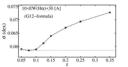
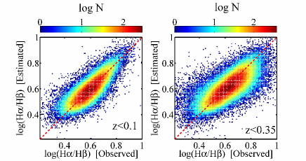
It is useful to begin our analysis with a test of the Balmer decrement prediction from Eq. 7 based on EWs extracted from the MPA/JHU catalogs, observed Petrosian magnitudes obtained from the SDSS and our own corrections to rest-frame quantities. Using Eq. 7, in Fig. 1 we plot the standard deviation between the predicted ratio of log(H$\alpha$/H$\beta$) and the observed ratio as a function of redshift. The top panel of Fig. 1 shows that the scatter agrees with that quoted by Groves et al. (2012) for $z<0.1$ and this EW range: $\sigma=0.058$ dex. However, for higher redshifts, the scatter in the comparison between the observed and predicted Balmer decrements increases steadily. This effect is highlighted in the lower two panels of Fig. 1 which compares the observed and predicted ratio of log(H$\alpha$/H$\beta$) in two redshift ranges, $z<0.1$ (left) and $z<0.35$ (right). These panels include all emission line galaxies with a S/N$>$3 (based on the criterion applied by Groves et al. 2012) in each of the H$\alpha$ and H$\beta$ lines. The colours and associated colour bar indicate the number of galaxies in each coloured point. We speculate that the decline in performance of Eq. 7 for our dataset might be caused by a difference in calculation of rest-frame colours. Regardless of the source of this redshift dependence, in order to fairly compare the performance of the ANN method and that of Groves et al. (2012), we simply restrict ourselves to the redshift range $z<0.1$.

Figure 1: The top panel: the standard deviation between the predicted log(H$\alpha$/H$\beta$) and observed ratio versus redshift. The horizontal dashed line shows scatter obtained by Equation 7 from Groves et al. (2012). The lower panels: the estimated log(H$\alpha$/H$\beta$) obtained from Equation 7 versus the value presented in the MPA/JHU catalogs for two cases, $z<0.1$ (left) and $z<0.35$ (right). The colours and associated colour bars indicate the number of galaxies in each coloured point.

3.1 The ANN and basis function approaches

We will now compare the performance of the ANN and also the basis function (polynomial) method to the same application, namely the prediction of the Balmer decrement based on the observed equivalent widths of H$\alpha$ and H$\beta$ and rest-frame $g-r$ colour. The artificial neural network is calibrated by sets of training data that are defined by the vector X_tr, see equation 2. For example, to replicate the input data of the Groves et al. (2012) analysis we define X₁=log(EW(H$\alpha))$, X₂=log(EW(H$\beta$)), X₃=$g$, and X₄=$r$, as four individual components of X_tr. These four components (N=4) can be also used in Equation 6 to find the 15 independent coefficients of this equation. At the start of the training procedure, the network must be initialized and the choice of the initialization parameters may affect the outcome of the trained network. We therefore repeat the training procedure 20 times with different initializations and average the results for the 10 best trained networks in terms of performance.

We begin with the same sample used by Groves et al. (2012) described above: all emission line galaxies in the SDSS DR7 in the MPA/JHU catalogs with H$\alpha$ and H$\beta$ S/N$>$3, which yields a sample of $\sim$ 95,000 galaxies. Of the $\sim$ 95,000 galaxies in the sample we randomly select half of them for training the network and the rest are used as a validation set. The validation step compares the performance of the ANN on target data (i.e. data not used in the training step) to ensure that accuracy is preserved in its application. A demonstration of the training and validation sets is shown in Section 7.1.

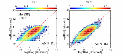
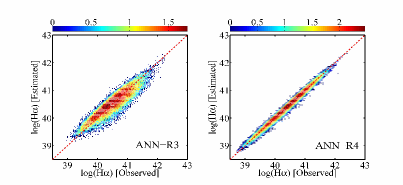
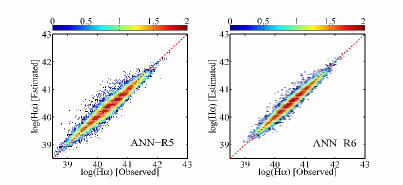
The ANN is set up with six different runs, which represent six different sets of training data. Although the default comparison with Groves et al. (2012) uses EW(H$\alpha)$, EW(H$\beta$), $g$ and $r$, it is instructive to investigate other parameter combinations. The data used in the input runs are listed in Table 1, where run R3 uses the same set of input data as Groves et al. (2012). Fig. 2 compares the performance of the ANN and basis function methods, with each row representing a different combination of input parameters, summarised by the runs in Table 1. The ANN predicted values are compared to those measured in the MPA/JHU catalogs in the right panels of Figure 2. The left panels show the results obtained from the basis function approach, denoted by f(x).

Table 1: Balmer decrement training runs; all magnitudes are extinction corrected, absolute, rest-frame and calculated within the SDSS fibre. EWs are in Å.

Runs	Input vectors (X)
R1	log(EW(H$\alpha$)), log(EW(H$\beta$))
R2	log(EW(H$\alpha$)), log(EW(H$\beta$)),$r$
R3	log(EW(H$\alpha$)), log(EW(H$\beta$)),$g,r$
R4	log(EW(H$\alpha$)), log(EW(H$\beta$)),$i,z$
R5	log(EW(H$\alpha$)), log(EW(H$\beta$)),log(M${}_{\rm fib}/M_{\odot})$
R6	log(EW(H$\alpha$)), log(EW(H$\beta$)),$u,g,r,i,z$

Figure 2: Each panel shows the value of log(H$\alpha$/H$\beta$) estimated from the basis function (left panel) and ANN (right panel) versus the measured value in the MPA/JHU catalog. The figure comprises the six different runs listed in Table 1. Run 3 uses the same input data as the calibration of Groves et al. (2012), using X₁=log(EW(H$\alpha))$ and X₂=log(EW(H$\beta$)), $g$, and $r$, i.e. the panel labelled ‘R3-ANN’ is directly comparable with Fig. 1. The colours and associated colour bars indicate the number of galaxies in each data point.

Figure 3: The standard deviation of the six different runs listed in Table 1 and shown in Fig. 2 for ANN (blue solid line) and the basis function (red dashed line). For comparison, the standard deviation of the Groves et al. (2012) calibration is shown as a horizontal dotted line. Runs whose standard deviations are below this line (R3 – R6) show a smaller scatter between the ANN predictions and measured values than Groves et al. (2012).

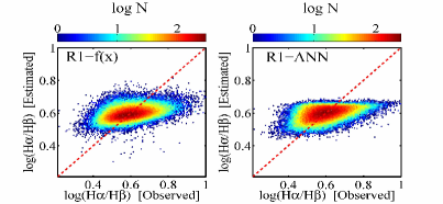
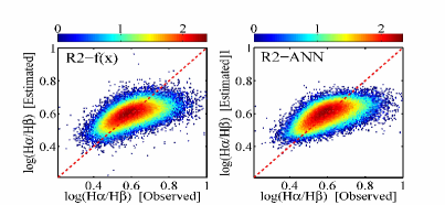
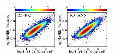
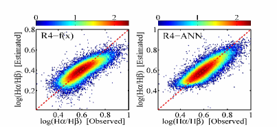
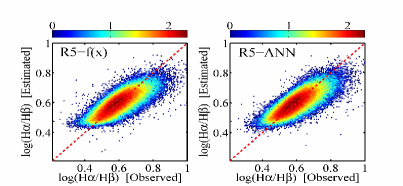
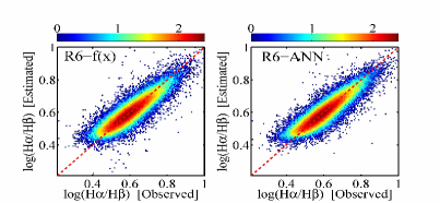
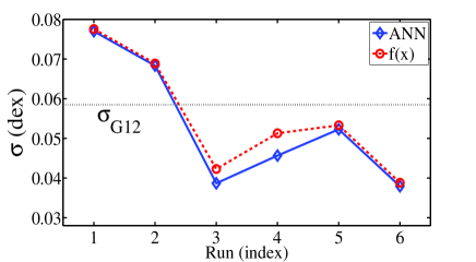
The top panel of Figure 2 (run R1) shows that an ANN with input data X₁=log(EW(H$\alpha$)) and X₂=log(EW(H$\beta$)) alone does not contain sufficient information to accurately reproduce the target value, H$\alpha$/H$\beta$. The standard deviation for this run is relatively large, almost 0.08 dex. Adding information about the brightness of the galaxy, in the case of run R2, the $r$-band absolute magnitude, does not significantly improve the situation. Run R3 has the same set of input data as the calibration of Groves et al. (2012): EW(H$\alpha$), EW(H$\beta$), $g$ and $r$ (absolute magnitudes) and now the third panel from top of Figure 2 shows a good correlation between the ANN prediction and measured Balmer decrement. As described by Groves et al. (2012), this is expected as the colour provides information on the stellar continuum. The standard deviation for run R3 using the ANN is 0.038 dex, compared to 0.058 dex for the Groves et al. (2012) predictions from equation 7 (Figure 1). Although this improvement is incremental, it does demonstrate the power and applicability of the ANN approach. The ANN also has the advantage of avoiding an explicit fit between continuum measured at the H${\alpha}$ and H${\beta}$ wavelengths and colour; the coefficients A₃ and A₄ are produced naturally as part of the ANN output. Run R4 substitutes $i$ and $z$-band magnitudes for the $g$ and $r$ used in R3; the correlation is still good ($\sigma$ = 0.046 dex), but not as good as in R3. Using the fibre stellar mass (also from the MPA/JHU catalog) instead of colour information also performs more poorly than R3 with a $\sigma=0.052$ dex. The run with the least scatter between the predicted and observed values is R6, which uses all 5 SDSS photometric bands. Run R6 performs marginally better than R3 with a standard deviation of 0.037 dex.

Figure 3 summarises the performance of each of the six runs; for each run the standard deviation between the predicted and measured Balmer decrement is plotted. The value of the Groves et al. (2012) calibration is shown for reference as a horizontal dotted line. The blue solid and red dashed lines show the result obtained from ANN and f(x), respectively. Figure 3 shows that runs R3 – R6 all yield lower scatter than the calibration of Groves et al. (2012). Figure 3 also shows that the scatter for each ANN run is slightly smaller than the result obtained by the basis function, although the difference is always less than 0.01 dex. The accuracy of predicted Balmer decrements obtained from both ANN and f(x) approaches can clearly match (or exceed) that of the formula presented by Groves et al. (2012).

The coefficients derived for runs R3 and R5 (the latter of which is useful in the absence of good optical photometry) are given below. All EWs are in Å. Due to the large number of coefficients, a matrix representation of Eq. 6 is most convenient. These coefficients therefore permit a straightforward analytic method for calculating the Balmer decrement. For run R3, with X as:

$$X=\left(\begin{array}[]{c}\rm{log~{}EW(H\alpha)}\\ \rm{log~{}EW(H\beta)}\\ \rm{g}\\ \rm{r}\\ \end{array}\right)$$

and where $f(C,X)=X^{T}CX+X^{T}C^{{}^{\prime}}+C^{{}^{\prime\prime}}$, C and C${}^{{}^{\prime}}$ are given by the following matrices:

$$C=\left(\begin{array}[]{rrrr}0.32005&-0.10277&0.14572&-0.14146\\ -0.10277&-0.03811&-0.08066&0.07727\\ 0.14572&-0.08066&-0.03282&0.03883\\ -0.14146&0.07727&0.03883&-0.04356\\ \end{array}\right)$$

$$C^{{}^{\prime}}=\left(\begin{array}[]{r}-0.38036\\ 0.11262\\ 0.32623\\ -0.30305\\ \end{array}\right)$$

and $C^{{}^{\prime\prime}}$=0.51103.

The scatter found using this relation to predict the Balmer decrement is $\sigma$=0.042 dex.

For run R5 with X as:

$$X=\left(\begin{array}[]{c}\rm{log~{}EW(H\alpha)}\\ \rm{log~{}EW(H\beta)}\\ \rm{log~{}(M_{fib}/M_{\odot})}\\ \end{array}\right)$$

The coefficients are:

$$C=\left(\begin{array}[]{rrr}0.09724&-0.05493&0.04130\\ -0.05493&-0.03587&-0.01420\\ 0.04130&-0.01420&0.02065\\ \end{array}\right)$$

$$C^{{}^{\prime}}=\left(\begin{array}[]{r}-0.74362\\ 0.29786\\ -0.39319\\ \end{array}\right)$$

$C^{{}^{\prime\prime}}=$2.28694, yielding a scatter of $\sigma=$0.053 dex.

The above formats are particularly well suited to matrix oriented software (such as IDL and MATLAB), although the coefficients $C_{ij}$, $C^{{}^{\prime}}_{i}$ and $C^{{}^{\prime\prime}}$ also can be directly used by considering the summation form of Eq. 6. For presentation purposes, we will present coefficients in the matrix format for the remainder of the paper.

4 The prediction of [NII] and H$\alpha$ luminosities in star-forming galaxies

After the demonstration in the previous section of our ANN technique, we now move to the main objective of the current work: a prediction of the H$\alpha$ and [NII]$\lambda 6584$ luminosities. The methodology is the same as in the previous section. First a series of training runs are established, each one with a different set of parameters to be used in the network. The training sets include half of the available number of galaxies. The other half is used in the verification phase, where we confirm that the ANN predicts the line luminosities with the expected scatter. Finally, in Section 6 and Appendix A, we provide analytic calibrations and matrix coefficients that represent the ANN output to be used by the general community.

We begin by considering only star forming galaxies in this section, but in the next section we go on to apply our technique to the general sample of emission line galaxies, regardless of their classification. The [NII]/H$\alpha$ ratios differ markedly between the star-forming and AGN populations due to the more significant contribution of forbidden lines in the presence of a hard ionizaing background. The different line flux ratios in star-forming regions compared with AGN forms the basis for many of the well-known AGN BPT classification schemes. When only star-forming galaxies are considered, there is a relatively tight relationship between the [OIII]/H$\beta$ ratio and that of [NII]/H$\alpha$, which is largely driven by a trend in metallicity (e.g. Dopita et al. 2006; Stasinska et al. 2006). This tight sequence, as we will see, lends itself to excellent predictions of [NII] and H$\alpha$ luminosities in star-forming galaxies.

In this section we select all galaxies from the SDSS that are classified as star-forming according to the calibration of Stasinska et al. (2006) and have available total and fibre stellar masses in the MPA/JHU catalog. Line fluxes have been corrected for Galactic extinction, but not internal extinction, since this is essentially calibrated as part of the ANN process. Before the imposition of any S/N requirements, these basic criteria yield 120,444 galaxies. Twelve separate training runs are established, containing between 1 and 8 parameters in different combinations, see Table 2. Each of the 11 runs between R2 and R12 requires at least one emission line so the ANN is tested separately for 3 different S/N criteria: S/N$>3$, S/N$>5$ and S/N$>8$. R1 uses only fibre stellar mass so does not need a S/N requirement. For a given S/N requirement, only the lines required as input in that run are required to pass the criterion. For example, in R2 only [OIII]$\lambda$ 5007 is required to pass the S/N criterion, and the same is true in run R5. However, in run R8, both [OIII]$\lambda$ 5007 and H$\beta$ are required to pass the criterion. Table 3 lists the number of galaxies in each sample, according to the run number and S/N threshold. Recall that half of these samples will be used in the ANN training process.

Table 2: The ANN run parameter combinations.

Runs	Input vectors log(X)
R1	M${}_{\rm{fib}}/M_{\odot}$
R2	OIII$\lambda$ 5007
R3	OII$\lambda$3727
R4	H$\beta$
R5	M${}_{\rm{fib}}/M_{\odot}$ + OIII$\lambda$5007
R6	M${}_{\rm{fib}}/M_{\odot}$ + OII$\lambda$3727
R7	M${}_{\rm{fib}}/M_{\odot}$ + H$\beta$
R8	M${}_{\rm{fib}}/M_{\odot}$ + OIII$\lambda$5007 + H$\beta$
R9	M${}_{\rm{fib}}/M_{\odot}$ + OII$\lambda$3727 + H$\beta$
R10	M${}_{\rm{fib}}/M_{\odot}$ + OIII$\lambda$5007+ OII$\lambda$3727 + H$\beta$
R11	R10+ OII$\lambda$3729, OIII$\lambda$4959
R12	R11+ SII$\lambda\lambda 6717,6731$

Table 3: The number of galaxies in each run with different S/N thresholds for star-forming galaxies.

Runs	Ngal (S/N$>3$)	Ngal (S/N$>5$)	Ngal (S/N$>8$)
R1	120444	120444	120444
R2	93365	69062	48249
R3	79309	50262	26660
R4	118383	110186	87838
R5	93365	69062	48249
R6	79309	50262	26660
R7	118383	110186	87838
R8	92970	68149	46169
R9	79268	50246	26650
R10	76329	48989	26309
R11	47368	29143	16481
R12	46910	28841	16270

The different training runs R1 – R12 are chosen to both provide insight into the most relevant parameters required for an accurate prediction of the [NII] and H$\alpha$ luminosities, but also with consideration of the most likely practical choices. For example, we investigate the impact of S/N on the ANN, and whether performance is improved when both members of a given doublet (such as [OII] $\lambda\lambda$ 3727, 3729) are used. Preference is given to relatively strong emission lines with blue rest wavelengths, under the assumption that these will be the most readily detectable in optical spectra. We do, however, include [SII] $\lambda\lambda$ 6716, 6731 in the last of the runs. Although this doublet is redwards of H$\alpha$ and [NII] $\lambda$ 6584, run R12 could potentially be useful in the case of one of the lines being contaminated, for example by telluric features. Mass is also included as an input parameter in some of the runs, due to its correlation with many other galaxy properties (such as SFR and metallicity) that in turn correlate with emission line strengths (or ratios).

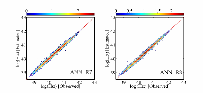
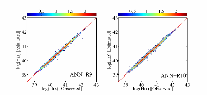
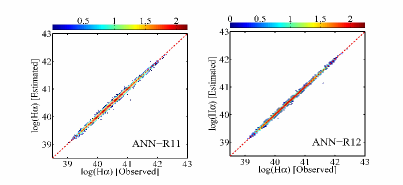
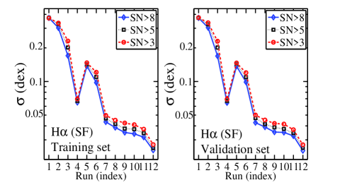
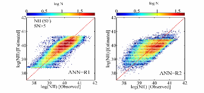
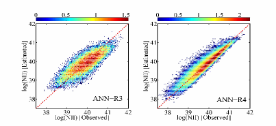
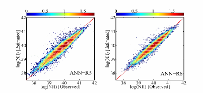
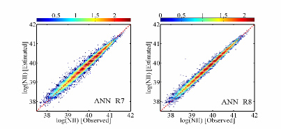
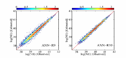
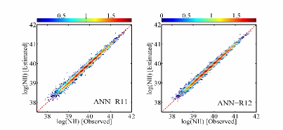
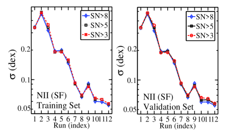
Figures 4 and 6 show the comparison of predicted versus measured H$\alpha$ and [NII] line luminosities, respectively. Only the S/N$>$5 runs are shown for brevity. In Figures 5 (H$\alpha$) and 7 ([NII]) a summary of the standard deviations is shown for each of the runs for all 3 S/N thresholds. Let us first consider the ANN’s performance in predicting the flux of the H$\alpha$ line (Figures 4 and 5). The first item of note is that the training and the validation sets are identically behaved (Figure 5) showing that the training of the network is robust and repeatable. As can be seen, from Figures 4 and 5, the physical parameter that is the single most important ingredient in the accurate prediction of the H$\alpha$ luminosity is, unsurprisingly, H$\beta$. All of the runs that include the H$\beta$ line have standard deviations $<$ 0.07 dex. Interestingly, the scatter varies little between the different S/N thresholds with less than 0.01 dex difference in the scatters between the S/N$>3$ and S/N$>8$ versions of a given run. Run R8 is perhaps one of the most useful combinations from a practical perspective, including two strong emission lines ([OIII] $\lambda$ 5007 and H$\beta$) that are relatively close in wavelength, plus fibre stellar mass. For this run, the ANN is able to predict the H$\alpha$ luminosity with a standard deviation of only 0.04 dex, even when the S/N threshold is as low as 3.

Figure 4: The ANN predicted H$\alpha$ luminosities compared to the observed values for the S/N$>$5 case for star-forming galaxies. The input data associated with each run are listed in Table 2. All the luminosities are in units of erg/s.

Figure 5: The standard deviation of the difference between estimated and observed H$\alpha$ for the training (left) and validation (right) sets for star-forming galaxies. The two sets show same behavior, indicating that the network is robust.

We turn next to the ANN predictions of [NII] $\lambda$6584 (Figures 6 and 7). Again, the training and validation sets are identical, demonstrating that the ANN’s results are robust and not dependent on the particular galaxies used in the training set. The standard deviations tend to be higher in general for the predictions of [NII] than for H$\alpha$. Interestingly, there is almost no dependence of the accuracy of the [NII] line prediction on the S/N of the training set. Although the dependence of the ANN’s performance is less dramatically linked to the use of H$\beta$ for predicting [NII] as it was for H$\alpha$, the H$\beta$ still appears to be the most important of the 3 strong emission lines used here ([OII], [OIII] and H$\beta$). Of the runs using a single emission line (R2 – R4), the latter, which uses H$\beta$ has the lowest scatter. Of the runs that combine mass and a single emission line (R5 – R7), again it is the latter which minimizes the scatter. As we saw was the case for the prediction of H$\alpha$, run R8, which is attractive for its practical combination of fibre stellar mass, H$\beta$ and [OIII]$\lambda$ 5007, has one of the smallest scatters ($\sim 0.07$ dex). Indeed, for both H$\alpha$ and [NII] the accuracy of the ANN’s prediction is improved little by adding [OII].

Figure 6: The ANN predicted [NII] $\lambda$ 6584 luminosities compared to the observed values for the S/N$>$5 case for star-forming galaxies. The input data associated with each run are listed in Table 2. All the luminosities are in units of erg/s.

Figure 7: The standard deviation of the difference between estimated and observed [NII]$\lambda$6584 for the training (left) and validation (right) sets for star-forming galaxies. The two sets show same behavior, indicating that the network is robust.

4.1 On the use of fibre vs. total stellar mass.

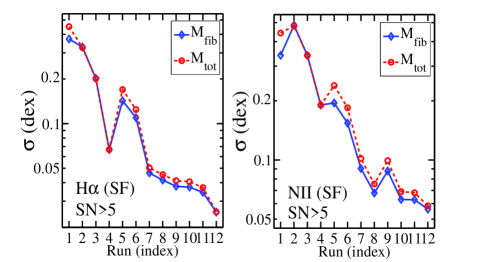
Up until now, we have used the fibre stellar mass under the assumption that predicting the spectral line strengths within a given aperture will be most sensitive to the mass enclosed in that same area. However, whilst total galaxy stellar masses might be readily available from broad-band photometry, determining aperture masses requires an additional analysis step. Therefore, in the spirit of user-friendliness, we investigate the impact of substituting total stellar mass instead of fibre mass in the runs listed in Table 2. In Figure 8 we compare the standard deviations of the 12 runs for the S/N $>$ 5 case with this mass substitution for both the H$\alpha$ and [NII] predictions (left and right panels respectively). Since some of the runs (R2, R3 and R4) do not use mass as an input parameter the substitution of total stellar mass for fibre stellar mass has no impact. For the other runs, we see that, as expected, the use of total stellar mass (red points) yields a slightly higher scatter, but the difference is typically $<0.01$ dex in the standard deviations. We conclude that total stellar mass can be used as a convenient alternative for aperture stellar mass, at least over the range of covering fractions probed by the SDSS data (typically 0.1 – 0.4). Nonetheless, we investigate explicitly in Section 7.1 the dependence of our calibrations on covering fraction.

Figure 8: A comparison between different runs (1-12) with total and fibre mass for S/N$>5$ for star-forming galaxies. Using the total stellar mass leads to a slightly enhanced scatter, although the difference is probably negligible for most applications.

5 The prediction of [NII] and H$\alpha$ luminosities for the general case of emission line galaxies

In the previous section, we demonstrated that an ANN can be successfully used to predict the H$\alpha$ and [NII] $\lambda$ 6584 line luminosities in star forming galaxies. In many cases, the accuracy of the luminosity prediction is within 0.1 dex. However, in practice, one can not always assume that the ionization of the interstellar medium is dominated by stars. Ionization by alternative sources, such as planetary nebulae, shocks or AGN will yield different line strengths. This fact forms the basis of diagnostic diagrams such as the BPT.

We therefore investigate whether the ANN is able to predict line luminosities for emission line galaxies whose dominant source of ionization is unknown. In practice, the two most likely sources to dominate in integrated spectra such as those from the SDSS are stars and AGN. In order to define a general sample of emission line galaxies, we therefore drop the first requirement in Section 4, that galaxies must be classified as star-forming. The full sample of galaxies is referred to as the ‘mixed’ sample, to reflect the combination of star-forming, AGN and other minority classes, such as LINERs. We repeat all of the ANN runs listed in Table 2, with the three S/N thresholds, and adopting the same strategy of splitting each sample into training and validation sets. Table 4 lists the number of galaxies in the mixed sample that is used in each of the different runs for the three S/N thresholds tested in the previous section.

Table 4: The number of galaxies in each run with different S/N thresholds for the mixed galaxies.

Runs	Ngal (S/N$>3$)	Ngal (S/N$>5$)	Ngal (S/N$>8$)
R1	264792	264792	264792
R2	189738	123768	79780
R3	122333	67686	33030
R4	212757	174502	126286
R5	189738	123768	79780
R6	122333	67686	33030
R7	212757	174502	126286
R8	166022	107014	65725
R9	120507	67306	32963
R10	116334	65633	32528
R11	67708	37242	19405
R12	67034	36858	19168

The scatter in the ANN predicted luminosities compared to the observed value for the mixed sample is shown in Figure 9, which includes the output from all three S/N cuts. Here, again, the validation and training sets show the same behavior so we only show the results from validation set. As can be seen, the difference in scatters for different S/N cuts is more significant than that of the star-forming sample, for both H$\alpha$ (Figure 5) and [NII] (Figure 7). The difference is more noticeable for H$\alpha$. This shows that the mixed sample (adding the AGN galaxies to the SF sample) can generate more complicated patterns in the dataset and these patterns have more dependency on the choice of S/N. From Figure 9, however, it seems that adding more information can give a more coherent result.

Figure 9: A comparison between different runs (1-12) with the ANN methods for the S/N$>5$ mixed galaxy sample. The left and the right panels are related to H$\alpha$ and [NII], respectively.

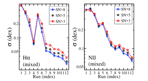
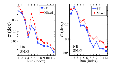
We compare again the use of fibre and total stellar masses. As was previously found for the star-forming galaxies, here also total stellar mass performs essentially as well as the fibre stellar mass. A direct comparison of the ANN’s performance between using only star-forming galaxies and including other classes is shown in Figure 10. As expected, the scatter is higher when all galaxy classes are included, but the ANN can still readily yield scatters $<$ 0.1 dex for both H$\alpha$ and [NII] for several of the runs. Again, the maximum information used as input data (run 12) yields the lowest scatter.

Figure 10: A comparison between different runs (1-12) with the ANN for the results obtained for SF (blue points) and mixed (red points) samples. The left and the right panels are related to H$\alpha$ and [NII], respectively.

6 Derivation of basis function coefficients

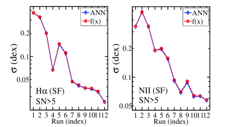
We now investigate how effectively the selected polynomial basis function (i.e., Eq. 6) can predict the results of the ANN. In Figure 11 we show a comparison between different runs (1-12) with the ANN and f(x) methods for S/N$>5$ in the star-forming sample. The left and the right panels are related to H$\alpha$ and [NII], respectively. There is an excellent match between the performance of the two methods, indicating that no accuracy is lost in the use of the polynomial.

Figure 11: A comparison between different runs (1-12) with ANN and f(x) methods for S/N$>5$ in the star-forming sample. The left and the right panels are related to H$\alpha$ and [NII], respectively.

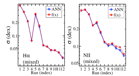
We repeat this exercise for the general case of emission line galaxies, which represents a mix of star-forming and AGN classes, with the results shown in Figure 12. The left panel, for estimating H$\alpha$, shows that the polynomial once again excellently reproduces the results of the ANN. However, the scatter in the [NII] line luminosity predictions is slightly higher when the polynomial is used, compared to the ANN, but the effect is very small, $<0.01$ dex.

Figure 12: A comparison between different runs (1-12) with ANN and f(x) methods for S/N$>5$. The left and the right panels are related to H$\alpha$ and [NII], respectively. In general, the basis function can accurately reproduce the ANN results.

In Appendix A we present all coefficients for estimating the H$\alpha$ and [NII] luminosities of star-forming and ‘mixed’ galaxies.

7 Testing the ANN calibration

In this section we test the robustness of the ANN calibration in three ways. First, we investigate the importance of the selected parameters used in ANN and the size and sampling of the training set. Second, we examine whether the scatter in predicted line luminosities depends on the physical parameters (such as mass and metallicity) of the sample. Finally, we test whether the calibrations derived for the SDSS data work well when applied to an independent dataset.

7.1 Size and sampling of the training set

A first consideration in the ANN application is the number of neurons used. For example, using a large number of the neurons in a network can increase its power, but it can also result in over-fitting. To prevent this, the networks’ parameters can be tuned in such a way that the training and validation sets show the same scatter. In the work presented here, we find that 8-10 neurons works well with our dataset. We also check several optimization algorithms and find that the Levenberg-Marquardt and Bayesian regulation back propagation provide the same results as one other, and are superior to other optimization algorithms such as a gradient descent back propagation.

The ANN will only work well if the training set is a good representation of the data for which the prediction is desired. The scatter in the training and validation sets also depends on the size of the training set. As mentioned previously, we repeat each run 20 times, with different initialization. For higher numbers of galaxies selected for training ANN the outputs of each run cover the same range. In other words, here, there is a stability. When we reduce the number of galaxies for training the output of the runs are in significantly different ranges. We find that a training sample of $>3000$ galaxies can predict an acceptable result in which the behavior of the training and validation sets are the same.

7.2 The effect of the physical parameters on estimated parameters

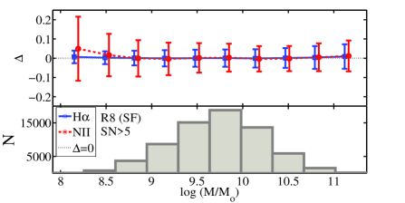
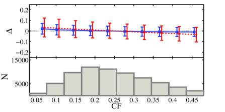
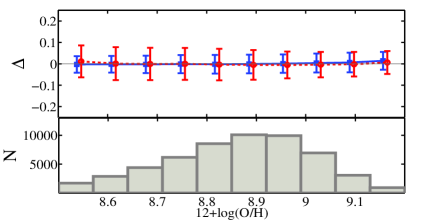
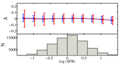
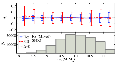
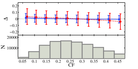
In Figures 13 and 14 we test the performance of the ANN as a function of various physical and observational parameters, for star-forming and mixed galaxies, respectively. In each figure we calculate the offset of the line luminosity predictions (of either H$\alpha$ or [NII]) relative to the observed luminosities as

$$\Delta=\rm{log(L_{pred}/L_{obs})}.$$ (8)

The blue lines in Figures 13 and 14 show the offsets for H$\alpha$ and the red lines show offsets for [NII]. In all panels of these two figures, we adopt the results of run R8 with a S/N$>$5 for demonstration purposes, although our conclusions do not depend on the choice of run.

For star-forming galaxies, we investigate in Figure 13, the difference in the predicted and observed line luminosities as a function of total stellar mass, $r$-band covering fraction (CF), metallicity and SFR. The $r$-band covering fraction is simply the fraction of light in the SDSS $r$-band that is included by the fibre, and is computed from the combination of total and fibre magnitudes.

From Figure 13 it can be seen that there is no systematic offset of $\Delta$ from zero as a function of total stellar mass or SFR for either H$\alpha$ or [NII]. The results are also equally robust to changes in the covering fraction, indicating that the calibrations provided in this paper may be applied to galaxies with a range of masses and obtained with a variety of apertures. Nonetheless, there is an extremely mild trend (although statistically insignificant) of $\Delta$ [NII] with covering fraction, such that the ANN slightly over-predicts the luminosity at large covering fractions, and slightly under-predicts the luminosity at the smallest apertures. The third panel of Figure 13 shows that this is unlikely to be due abundance gradients, since $\Delta$ again shows no strong dependence on O/H.

Similar trends are seen for the mixed sample of star-forming plus AGN galaxies in Figure 14: there is no trend of $\Delta$ H$\alpha$ with total stellar mass, although the scatter is larger. The larger scatter is to be expected from Figure 10 where we have shown that the mixed class has a higher scatter in H$\alpha$ and [NII] for most of the runs, compared with the star-forming only sample. The same mild, though statistically insignificant, trend is seen with covering fraction. No comparison is done for metallicity or SFR in the mixed sample, since the presence of an AGN negates the application of strong line metallicity and SFR calibrations.

We conclude that the calibrations presented in this paper show no systematic deviations as a function of stellar mass, SFR, covering fraction or metallicity, and should hence be applicable to a wide range of observed data.

Figure 13: The difference in the estimated and observed parameters H$\alpha$ and [NII] vs. total stellar mass, covering fraction (CF), metallicity and SFR, for star forming galaxies

Figure 14: The difference in the estimated and observed parameters H$\alpha$ and [NII] vs. total stellar mass and covering fraction (CF), for the mixed galaxies.

7.3 Application to an independent dataset

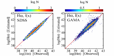
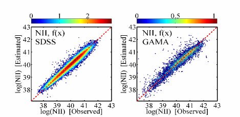
In order to test the assertion of the previous subsection, we now demonstrate the applicability of the calibrations we have derived in this work to another dataset. Specifically, we will use the publicly available data of the Galaxy and Mass Assembly (GAMA) survey. The GAMA survey is a joint European-Australasian project based around a spectroscopic campaign using the Anglo-Australian Telescope (AAT). The GAMA target catalogue is based on selection from the SDSS (Baldry et al. 2010; Robotham et al. 2010), but provides independent spectroscopy and derived data products (e.g. Driver et al. 2011; Hill et al. 2011; Taylor et al. 2011). We compile emission line fluxes, redshifts and fibre stellar masses from the publicly available GAMA data release 2. Total stellar masses are derived using the GAMA-provided flux scales appropriate to our cosmology (Taylor et al., 2011). Balmer emission line fluxes have already been corrected for underlying stellar absorption. We impose a redshift cut $z>0.003$ in order to avoid stellar confusion.

In order to test the application of the basis function coefficients presented in Appendix A, we select a sample of mixed emission line galaxies from GAMA that are consistent with the requirements of run R8. That is, we select the $\sim$ 8000 GAMA galaxies with well determined stellar masses and with emission lines [OIII] and H$\beta$ having S/N$>$3. The predicted line luminosities of H$\alpha$ (upper panel) and [NII] (lower panel) obtained from Eq. 6, f(x), are shown in the right hand panels of Figure 15. For a comparison, we plot the results obtained with the SDSS data set in the left panels. The two datasets show a similar behavior, although the GAMA data set shows a slightly larger scatter ($\sim 0.05$ dex) compared to the SDSS. A small fraction of GAMA sample ($\sim 1\%$) have very large offsets. In the SDSS data set, this kind of offset is not seen in the validation and training sets for either the ANN method nor for the f(x) method. It is likely that the high scatter is due (at least in part) to the different methods and accuracies of calibration, data processing and stellar mass determination. For example, the GAMA data show a higher mean value for the two input emission lines and an average 0.25 dex difference in the stellar masses. Despite these differences, and the differences that are likely inherent to other datasets, Figure 15 demonstrates that the methods presented here yield generally very good line luminosity predictions. However, we close this section with one final caveat. The ANN-based calibrations that we have presented in this paper were obtained using a low redshift training set (the SDSS). At high redshifts (above 1.0 – 1.5), it seems likely that the pattern of line ratios on which the ANN relies will change (Liu et al. 2008; Brinchmann et al. 2008; Kewley et al. 2013b), and the calibrations presented here are likely to not be applicable.

Figure 15: A comparison between data taken from SDSS (left panels) and GAMA (right panels) using the f(x) method for run R8. The top and the bottom panels are related to H$\alpha$ and [NII], respectively. All the luminosities are in units of erg/s.

8 Example applications of line luminosity predictions

Having tested the robustness of the ANN method, in this final section, we provide two example applications of the line luminosity predictions.

8.1 Constructing the BPT diagram

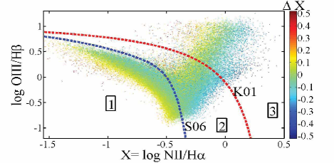
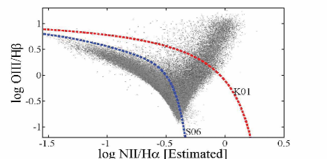
The BPT diagram is an important tool for distinguishing AGN and SF galaxies from each other. To demonstrate the application of our method (which we have shown works well for both star-forming and AGN dominated galaxies) in this regard, we compare the [NII] and H${\alpha}$ of the observed (original) data with those that are predicted by our method and construct two BPT diagrams. The top panel of Figure 16 shows a BPT diagram that is constructed for Run 8 for the mixed sample. The horizontal axis shows the observed value of log (NII/H${\alpha}$) as X. The points are colour-coded by $\Delta$X = log (NII/H${\alpha})_{(pred)}$ - log (NII/H${\alpha})_{(obs)}$. Almost all [NII]/H$\alpha$ line ratios are predicted within $\Delta X<0.2$ dex and $\sigma\sim 0.1$ dex. The dotted red and blue lines indicate the demarcation lines given by Kewley et al. (2001) (K01), and Stasinska et al. (2006) (S06), respectively. We thus label three classes in the plot: Class 1=SF, Class2=composite, Class3=AGN, for use in the confusion matrix (described below). The middle panel shows the BPT diagram obtained when we use the predicted values of NII/H$\alpha$.

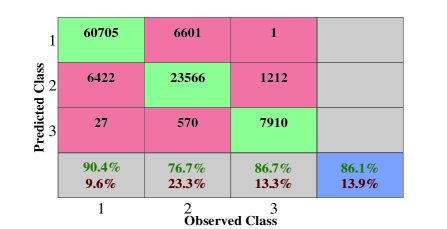
The bottom panel of Figure 16 shows the confusion matrix, which quantifies how well the predicted [NII] and H${\alpha}$ luminosities translate to correct AGN classifications. The numbers in the squares of the confusion matrix indicate the number of galaxies thus classified. Rows represent the predicted class (1, 2 or 3) and columns represent the actual observed class. For example, if column 1 is added up (60705+6422+27), the total number of galaxies in class1 (star-forming) is obtained. The green squares show the numbers of galaxies whose predicted class is the same as the observed class. The 6 red boxes give the numbers of galaxies incorrectly classified. For example, only one galaxy is mis-classified from class3 to class1, whereas 27 galaxies go from class1 to class3 and so on. In the bottom row, the green and red values give the percentages of galaxies correctly or incorrectly (respectively) classified for a given class. For example, 90.4 per cent of SF galaxies are correctly classified; 9.6$\%$ of the SF galaxies go to other classes. The blue block shows that 86.1$\%$ of galaxies in all classes are correctly placed, demonstrating the successful application of our method for AGN classifications.

Figure 16: Top plot: The BPT diagram associated with Run 8. The horizontal axis shows the observed value of log ([NII]/H${\alpha}$) as X. The points are colour-coded as $\Delta$X = log ([NII]/H${}_{\alpha})_{(pred)}$ - log ([NII]/H${\alpha})_{(obs)}$. The dotted red and blue lines indicate the demarcation lines given by K01, and S06. The middle panel shows the BPT diagram when we use the predicted value of [NII]/H${\alpha}$. The difference between the two BPT diagrams is represented in the bottom panel as a confusion matrix. 86 per cent of SDSS galaxies are correctly classified. See text for more explanation.

8.2 Metallicity calibrations and conversions

There are many metallicity calibrations that have been developed from different methodologies and datasets. Kewley & Ellison (2008) investigate the SDSS mass-metallicity relation with 10 different metallicity calibrations, encompassing those based on both theoretical and empirical methods. Several of these methods are variants on the R₂₃ method, requiring [OII] $\lambda$ 3727, [OIII] $\lambda$ 4959, [OIII$]\lambda$ 5007 and H$\beta$ (e.g., Kobulnicky & Kewley 2004, KK04). R₂₃ diagnostics have the advantage of requiring only 3 emission lines spanning a relatively narrow wavelength range. The well-known principal disadvantage of R₂₃ calibrations is the need to break the degeneracy between upper and lower branches. [NII] is frequently used to achieve this (e.g. Kewley & Ellison 2008), so one application of the line predictions presented in this work is to break this degeneracy.

A second metallicity application of the predictions presented herein involves conversions between metallicity indicators. As demonstrated by Kewley & Ellison (2008), the factor of five spread in metallicity between calibrations may hinder the combination of different datasets. Kewley & Ellison therefore derive polynomial fits between metallicities derived from different calibrations, which can be used to convert between diagnostics. However, an alternative to converting via the Kewley & Ellison polynomials, is to predict the additional line fluxes needed to calculate the metallicity in the desired diagnostic.

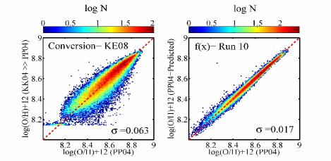
As an example, we consider the case where we would like to convert an R₂₃ based calibration to one which uses [NII] and H$\alpha$, (e.g., Pettini & Pagel 2004, PP04). We use Run 10 in this demonstration, since it combines the emission lines used in the basic R₂₃ diagnostic. We will consider the PP04 metallicity as our ‘target’ metallicity, but imagine the case where only [OII] $\lambda$ 3727, [OIII] $\lambda$ 4959, [OIII$]\lambda$ 5007 and H$\beta$ are observed. We begin by adopting the predictive approach described in this paper, namely we predict the [NII] and H$\alpha$ luminosities using the polynomial functions described in Section 6 for Run 10, and can hence calculate PP04 metallicities. It is of course possible to calculate real PP04 metallicities for our sample, since the SDSS data have measured values of [NII] and H$\alpha$. We can hence compare the PP04 metallicities measured in the data, with that based on predicted [NII] and H$\alpha$ line luminosities. The right panel of Figure 17 compares the predicted and measured PP04 metallicities. Clearly, the agreement is excellent, with small scatter (0.017 dex) and very few outliers.

Alternatively, we can repeat our experiment that begins with the observed [OII] $\lambda$ 3727, [OIII] $\lambda$ 4959, [OIII$]\lambda$ 5007 and H$\beta$, and first calculate an R₂₃ metallicity. We adopt the KK04 calibration for this test. We can then use the conversion in Kewley & Ellison (2008) to determine the equivalent PP04 metallicity. The result is shown in the left panel of Figure 17. The horizontal axis is the same as the right panel, namely the PP04 metallicity that can be determined directly from the data. The vertical axis is now the metallicity of PP04 that has been converted from KK04. Although the overall correlation is good, the scatter is larger (0.063 dex) and there are some cases (albeit a minority) where the conversion fails (see the region of converted metallicities of log O/H + 12 $\sim$ 8.2). Whilst the conversions of Kewley & Ellison (2008) are still advantageous in cases where line fluxes are not provided (i.e. only metallicities are quoted), the more complex relations encapsulated by the ANN-based calibrations offer an alternative route to robust metallicity conversions.

Figure 17: In both panels, the measured metallicity from the PP04 diagnostic is shown on the x-axis. This is compared, in the left panel, with the PP04 metallicity derived from the KK04 R₂₃ diagnostic plus the conversion given in Kewley & Ellison (2008). The right panel shows the case in which the PP04 metallicity is obtained using Run 10 and the polynomial-based prediction of [NII] and H$\alpha$. The ANN-based approach yields a much tighter relation with the directly measured metallicities.

9 Conclusions

Artificial neural networks (ANNs) can be used to predict spectral line luminosities that are useful for a variety of applications. After an overview of formalism of the ANN, we present a simple case study for the prediction of the Balmer decrement (H$\alpha$/H$\beta$) which is compared to the analytic prediction of Groves et al. (2012). Since the ANN predicts the expected observed (rather than intrinsic) line luminosity, our prediction of H$\alpha$ can be combined with the actual observed H$\beta$ in order to determine the galaxy’s internal extinction. We show that using the same input data, we can decrease the scatter in the predictions of the decrement from 0.058 (Groves et al. 2012) to 0.038 dex (ANN).

We then present an application of artificial neural networks to the prediction of H$\alpha$ and [NII] $\lambda$ 6584 luminosities in galaxy spectra. The ANN is trained on large samples (many tens of thousands) of galaxies from the SDSS, and tested for biases in training sample size, galaxy properties and aperture covering fraction. Twelve runs with different input parameters are tested, representing varying combinations of stellar masses and strong emission lines. Many of the runs can predict line luminosities with scatters $<$ 0.1 dex, regardless of whether the galaxy is star-forming or has an AGN and whether total or fibre stellar mass is used. These results indicate that the ANN is a robust tool for predicting the line luminosity of H$\alpha$ and [NII] in low redshift galaxies. Indeed, testing on an independent dataset (GAMA) yields scatter in the line luminosities only $\sim$ 0.05 dex larger than the SDSS data set, likely due to different calibration/reduction procedures.

In order to demonstrate potential applications of our method, we investigate the measurement of gas-phase metallicities and AGN classification. The ANN yields a considerable improvement in the prediction of gas-phase metallicities from diagnostics that require the [NII] and H$\alpha$ lines, compared to the empirically determined conversions of Kewley & Ellison (2008) and an AGN classification is successful in 86 per cent of SDSS galaxies.

In order to make the ANN results useful to the general community, we have derived polynomial basis function coefficients in a condensed matrix form that accurately reproduces the ANN results.

Appendix A The coefficients of the basis function

Here, we present the coefficients of Eq. 6 for star-forming and mixed galaxies for all of the runs of Table 2. In each case we have: $f(C,X)=X^{T}CX+X^{T}C^{{}^{\prime}}+C^{{}^{\prime\prime}}$. We present the result for the S/N$>5$ cut, although as shown in this paper, the dependence on S/N is not large. We first present the coefficients for star-forming galaxies in Sections A.1 and A.2 for H$\alpha$ and [NII], respectively. The coefficients for H$\alpha$ and [NII] in the mixed galaxies are in Sections A.3 and A.4. In all cases, the masses are total values and are in units of solar masses and luminosities are in units of erg/s.

A.1 Star forming galaxies, H$\alpha$

A.1.1 Run 1

$$X=\left(\begin{array}[]{c}\rm{log}(M_{tot}/M_{\odot})\\ \end{array}\right)$$

$$C=\left(\begin{array}[]{rrr}-0.03296\\ \end{array}\right)$$

$$C^{{}^{\prime}}=\left(\begin{array}[]{r}1.24672\\ \end{array}\right)$$

$C^{{}^{\prime\prime}}$= 31.25272

$\sigma$=0.460 dex

A.1.2 Run 2

$$X=\left(\begin{array}[]{c}\rm{log}~{}L(OIII)\lambda 5007\\ \end{array}\right)$$

$$C=\left(\begin{array}[]{rrr}-0.15360\\ \end{array}\right)$$

$$C^{{}^{\prime}}=\left(\begin{array}[]{r}13.10619\\ \end{array}\right)$$

$C^{{}^{\prime\prime}}$= -237.75141

$\sigma=$0.328 dex

A.1.3 Run 3

$$X=\left(\begin{array}[]{c}\rm{log}~{}L(OII)\lambda 3727\\ \end{array}\right)$$

$$C=\left(\begin{array}[]{rrr}-0.09694\\ \end{array}\right)$$

$$C^{{}^{\prime}}=\left(\begin{array}[]{r}8.87324\\ \end{array}\right)$$

$C^{{}^{\prime\prime}}$= -159.23380

$\sigma=$0.202 dex

A.1.4 Run 4

$$X=\left(\begin{array}[]{c}\rm{log}~{}L(H\beta)\\ \end{array}\right)$$

$$C=\left(\begin{array}[]{rrr}-0.01622\\ \end{array}\right)$$

$$C^{{}^{\prime}}=\left(\begin{array}[]{r}2.34114\\ \end{array}\right)$$

$C^{{}^{\prime\prime}}$= -27.09286

$\sigma=$0.067 dex

A.1.5 Run 5

$$X=\left(\begin{array}[]{c}\rm{log}(M_{tot}/M_{\odot})\\ \rm{log}~{}L(OIII)\lambda 5007\\ \end{array}\right)$$

$$C=\left(\begin{array}[]{rrr}-0.02273&-0.02675\\ -0.02675&-0.05434\\ \end{array}\right)$$

$$C^{{}^{\prime}}=\left(\begin{array}[]{r}3.14945\\ 5.59911\\ \end{array}\right)$$

$C^{{}^{\prime\prime}}=$-103.99888

$\sigma=$0.174 dex

A.1.6 Run 6

$$X=\left(\begin{array}[]{c}\rm{log}(M_{tot}/M_{\odot})\\ \rm{log}~{}L(OII)\lambda 3727\\ \end{array}\right)$$

$$C=\left(\begin{array}[]{rrr}0.15201&-0.07548\\ -0.07548&0.00162\\ \end{array}\right)$$

$$C^{{}^{\prime}}=\left(\begin{array}[]{r}3.44755\\ 2.25416\\ \end{array}\right)$$

$C^{{}^{\prime\prime}}=$-41.39747

$\sigma=$0.129 dex

A.1.7 Run 7

$$X=\left(\begin{array}[]{c}\rm{log}(M_{tot}/M_{\odot})\\ \rm{log}~{}L(H\beta)\\ \end{array}\right)$$

$$C=\left(\begin{array}[]{rrr}0.01016&-0.00472\\ -0.00472&-0.00085\\ \end{array}\right)$$

$$C^{{}^{\prime}}=\left(\begin{array}[]{r}0.26847\\ 1.15591\\ \end{array}\right)$$

$C^{{}^{\prime\prime}}=$-4.20487

$\sigma$=0.051 dex

A.1.8 Run 8

$$X=\left(\begin{array}[]{c}\rm{log}(M_{tot}/M_{\odot})\\ \rm{log}~{}L(OIII)\lambda 5007\\ \rm{log}~{}L(H\beta)\\ \end{array}\right)$$

$$C=\left(\begin{array}[]{rrr}0.03111&-0.01046&-0.01025\\ -0.01046&-0.00021&-0.00688\\ -0.01025&-0.00688&0.02283\\ \end{array}\right)$$

$$C^{{}^{\prime}}=\left(\begin{array}[]{r}1.12673\\ 0.72863\\ -0.04120\\ \end{array}\right)$$

$C^{{}^{\prime\prime}}=$1.09006

$\sigma=$0.046 dex

A.1.9 Run 9

$$X=\left(\begin{array}[]{c}\rm{log}(M_{tot}/M_{\odot})\\ \rm{log}~{}L(OII)\lambda 3727\\ \rm{log}~{}L(H\beta)\\ \end{array}\right)$$

$$C=\left(\begin{array}[]{rrr}0.02220&-0.00141&-0.00747\\ -0.00141&-0.08002&0.08326\\ -0.00747&0.08326&-0.08025\\ \end{array}\right)$$

$$C^{{}^{\prime}}=\left(\begin{array}[]{r}0.34978\\ -0.36266\\ 1.02108\\ \end{array}\right)$$

$C^{{}^{\prime\prime}}=$5.64838

$\sigma$=0.042 dex

A.1.10 Run 10

$$X=\left(\begin{array}[]{c}\rm{log}(M_{tot}/M_{\odot})\\ \rm{log}~{}L(OII)\lambda 3727\\ \rm{log}~{}L(OIII)\lambda 5007\\ \rm{log}~{}L(H\beta)\\ \end{array}\right)$$

$$C=\left(\begin{array}[]{rrrr}0.02388&-0.00471&-0.00838&-0.00002\\ -0.00471&0.02498&-0.01381&0.00751\\ -0.00838&-0.01381&-0.06316&0.07245\\ -0.00002&0.00751&0.07245&-0.08338\\ \end{array}\right)$$

$$C^{{}^{\prime}}=\left(\begin{array}[]{r}0.65118\\ -1.56593\\ 0.51798\\ 1.42717\\ \end{array}\right)$$

$C^{{}^{\prime\prime}}$=9.82980

$\sigma$=0.041 dex

A.1.11 Run 11

$$X=\left(\begin{array}[]{c}\rm{log}(M_{tot}/M_{\odot})\\ \rm{log}~{}L(OII)\lambda 3727\\ \rm{log}~{}L(OII)\lambda 3729\\ \rm{log}~{}L(OIII)\lambda 4959\\ \rm{log}~{}L(OIII)\lambda 5007\\ \rm{log}~{}L(H\beta)\\ \end{array}\right)$$

$$C=\left(\begin{array}[]{rrrrrr}0.00849&-0.01119&-0.02542&-0.00758&-0.00338&0.04340\\ -0.01119&0.24333&-0.28838&0.00784&0.03451&-0.00215\\ -0.02542&-0.28838&0.18608&0.16751&-0.15217&0.08324\\ -0.00758&0.00784&0.16751&-0.18046&0.07107&-0.05579\\ -0.00338&0.03451&-0.15217&0.07107&-0.08688&0.13757\\ 0.04340&-0.00215&0.08324&-0.05579&0.13757&-0.17301\\ \end{array}\right)$$

$$C^{{}^{\prime}}=\left(\begin{array}[]{r}0.22781\\ 0.55526\\ 0.75596\\ -0.92821\\ -0.09195\\ 1.13597\\ \end{array}\right)$$

$C^{{}^{\prime\prime}}$=-9.22439

$\sigma$=0.037 dex

A.1.12 Run 12

$$X=\left(\begin{array}[]{c}\rm{log}(M_{tot}/M_{\odot})\\ \rm{log}~{}L(OII)\lambda 3727\\ \rm{log}~{}L(OII)\lambda 3729\\ \rm{log}~{}L(OIII)\lambda 4959\\ \rm{log}~{}L(OIII)\lambda 5007\\ \rm{log}~{}L(H\beta)\\ \rm{log}~{}L(SII)\lambda 6717\\ \rm{log}~{}L(SII)\lambda 6731\\ \end{array}\right)$$

$$C=\left(\begin{array}[]{rrrrrrrr}0.00968&-0.02743&-0.01413&0.00426&0.00049&0.03736&0.05072&-0.05871\\ -0.02743&0.07812&-0.02066&0.00922&-0.08175&0.23562&-0.21780&0.00315\\ -0.01413&-0.02066&0.02049&0.01218&-0.05831&0.08275&0.25872&-0.30051\\ 0.00426&0.00922&0.01218&-0.3118&0.31590&-0.11115&0.18424&-0.09006\\ 0.00049&-0.08175&-0.05831&0.31590&-0.15913&-0.08423&-0.10801&0.16496\\ 0.03736&0.23562&0.08275&-0.11115&-0.08423&0.35655&-0.49776&-0.00398\\ 0.05072&-0.21780&0.25872&0.18424&-0.10801&-0.49776&-0.44227&0.80051\\ -0.05871&0.00315&-0.30051&-0.09006&0.16496&-0.00398&0.80051&-0.52487\\ \end{array}\right)$$

$$C^{{}^{\prime}}=\left(\begin{array}[]{r}0.40251\\ -0.11074\\ 0.41208\\ -1.06788\\ 1.33069\\ 1.47554\\ 1.53207\\ -2.62153\\ \end{array}\right)$$

$C^{{}^{\prime\prime}}$=-1.41523

$\sigma$=0.026 dex

A.2 Star forming galaxies, NII

A.2.1 Run 1

$$X=\left(\begin{array}[]{c}\rm{log}(M_{tot}/M_{\odot})\\ \end{array}\right)$$

$$C=\left(\begin{array}[]{rrr}-0.16813\\ \end{array}\right)$$

$$C^{{}^{\prime}}=\left(\begin{array}[]{r}4.13524\\ \end{array}\right)$$

$C^{{}^{\prime\prime}}$= 15.37728

$\sigma$=0.452 dex

A.2.2 Run 2

$$X=\left(\begin{array}[]{c}\rm{log}~{}L(OIII)\lambda 5007\\ \end{array}\right)$$

$$C=\left(\begin{array}[]{rrr}-0.22813\\ \end{array}\right)$$

$$C^{{}^{\prime}}=\left(\begin{array}[]{r}19.00561\\ \end{array}\right)$$

$C^{{}^{\prime\prime}}$= -355.07588

$\sigma=$0.485 dex

A.2.3 Run 3

$$X=\left(\begin{array}[]{c}\rm{log}~{}L(OII)\lambda 3727\\ \end{array}\right)$$

$$C=\left(\begin{array}[]{rrr}-0.20077\\ \end{array}\right)$$

$$C^{{}^{\prime}}=\left(\begin{array}[]{r}17.26172\\ \end{array}\right)$$

$C^{{}^{\prime\prime}}$= -329.24057

$\sigma=$0.341 dex

A.2.4 Run 4

$$X=\left(\begin{array}[]{c}\rm{log}~{}L(H\beta)\\ \end{array}\right)$$

$$C=\left(\begin{array}[]{rrr}-0.08098\\ \end{array}\right)$$

$$C^{{}^{\prime}}=\left(\begin{array}[]{r}7.59421\\ \end{array}\right)$$

$C^{{}^{\prime\prime}}$= -134.11928

$\sigma=$0.191 dex

A.2.5 Run 5

$$X=\left(\begin{array}[]{c}\rm{log}(M_{tot}/M_{\odot})\\ \rm{log}~{}L(OIII)\lambda 5007\\ \end{array}\right)$$

$$C=\left(\begin{array}[]{rrr}-0.15073&0.00102\\ 0.00102&-0.09215\\ \end{array}\right)$$

$$C^{{}^{\prime}}=\left(\begin{array}[]{r}3.71279\\ 7.98303\\ \end{array}\right)$$

$C^{{}^{\prime\prime}}=$-154.44567

$\sigma=$0.244 dex

A.2.6 Run 6

$$X=\left(\begin{array}[]{c}\rm{log}(M_{tot}/M_{\odot})\\ \rm{log}~{}L(OII)\lambda 3727\\ \end{array}\right)$$

$$C=\left(\begin{array}[]{rrr}-0.00206&-0.02532\\ -0.02532&-0.06718\\ \end{array}\right)$$

$$C^{{}^{\prime}}=\left(\begin{array}[]{r}2.73641\\ 6.69499\\ \end{array}\right)$$

$C^{{}^{\prime\prime}}=$-127.06397

$\sigma=$0.189 dex

A.2.7 Run 7

$$X=\left(\begin{array}[]{c}\rm{log}(M_{tot}/M_{\odot})\\ \rm{log}~{}L(H\beta)\\ \end{array}\right)$$

$$C=\left(\begin{array}[]{rrr}-0.15371&0.03475\\ 0.03475&-0.03697\\ \end{array}\right)$$

$$C^{{}^{\prime}}=\left(\begin{array}[]{r}0.60523\\ 3.20966\\ \end{array}\right)$$

$C^{{}^{\prime\prime}}=$-47.62000

$\sigma$=0.103 dex

A.2.8 Run 8

$$X=\left(\begin{array}[]{c}\rm{log}(M_{tot}/M_{\odot})\\ \rm{log}~{}L(OIII)\lambda 5007\\ \rm{log}~{}L(H\beta)\\ \end{array}\right)$$

$$C=\left(\begin{array}[]{rrr}0.05580&0.04715&-0.09749\\ 0.04715&-0.38793&0.37129\\ -0.09749&0.37129&-0.33060\\ \end{array}\right)$$

$$C^{{}^{\prime}}=\left(\begin{array}[]{r}3.08934\\ -0.16444\\ 0.23358\\ \end{array}\right)$$

$C^{{}^{\prime\prime}}=$2.50062

$\sigma=$0.077 dex

A.2.9 Run 9

$$X=\left(\begin{array}[]{c}\rm{log}(M_{tot}/M_{\odot})\\ \rm{log}~{}L(OII)\lambda 3727\\ \rm{log}~{}L(H\beta)\\ \end{array}\right)$$

$$C=\left(\begin{array}[]{rrr}-0.16622&0.03788&0.01900\\ 0.03788&-0.50049&0.43634\\ 0.01900&0.43634&-0.43066\\ \end{array}\right)$$

$$C^{{}^{\prime}}=\left(\begin{array}[]{r}-1.02627\\ 3.84885\\ 0.63659\\ \end{array}\right)$$

$C^{{}^{\prime\prime}}=$-64.41316

$\sigma$=0.103 dex

A.2.10 Run 10

$$X=\left(\begin{array}[]{c}\rm{log}(M_{tot}/M_{\odot})\\ \rm{log}~{}L(OII)\lambda 3727\\ \rm{log}~{}L(OIII)\lambda 5007\\ \rm{log}~{}L(H\beta)\\ \end{array}\right)$$

$$C=\left(\begin{array}[]{rrrr}0.04888&-0.03780&0.06129&-0.05993\\ -0.03780&-0.02406&0.06520&-0.01936\\ 0.06129&0.06520&-0.53989&0.47404\\ -0.05993&-0.01936&0.47404&-0.45100\\ \end{array}\right)$$

$$C^{{}^{\prime}}=\left(\begin{array}[]{r}2.09873\\ -1.22501\\ -1.67510\\ 2.62808\\ \end{array}\right)$$

$C^{{}^{\prime\prime}}$=14.47485

$\sigma$=0.070 dex

A.2.11 Run 11

$$X=\left(\begin{array}[]{c}\rm{log}(M_{tot}/M_{\odot})\\ \rm{log}~{}L(OII)\lambda 3727\\ \rm{log}~{}L(OII)\lambda 3729\\ \rm{log}~{}L(OIII)\lambda 4959\\ \rm{log}~{}L(OIII)\lambda 5007\\ \rm{log}~{}L(H\beta)\\ \end{array}\right)$$

$$C=\left(\begin{array}[]{rrrrrr}0.01892&-0.05874&-0.02687&0.04600&0.01915&0.00109\\ -0.05874&0.32541&-0.49221&-0.04912&0.24652&-0.03436\\ -0.02687&-0.49221&0.40693&0.21087&-0.24713&0.09164\\ 0.04600&-0.04912&0.21087&-0.74986&0.52075&0.03981\\ 0.01915&0.24652&-0.24713&0.52075&-0.99480&0.52839\\ 0.00109&-0.03436&0.09164&0.03981&0.52839&-0.62532\\ \end{array}\right)$$

$$C^{{}^{\prime}}=\left(\begin{array}[]{r}1.34917\\ 1.36630\\ 2.70244\\ 0.47628\\ -4.52718\\ 1.91962\\ \end{array}\right)$$

$C^{{}^{\prime\prime}}$=-25.86109

$\sigma$=0.069 dex

A.2.12 Run 12

$$X=\left(\begin{array}[]{c}\rm{log}(M_{tot}/M_{\odot})\\ \rm{log}~{}L(OII)\lambda 3727\\ \rm{log}~{}L(OII)\lambda 3729\\ \rm{log}~{}L(OIII)\lambda 4959\\ \rm{log}~{}L(OIII)\lambda 5007\\ \rm{log}~{}L(H\beta)\\ \rm{log}~{}L(SII)\lambda 6717\\ \rm{log}~{}L(SII)\lambda 6731\\ \end{array}\right)$$

$$C=\left(\begin{array}[]{rrrrrrrr}0.01942&-0.04737&-0.03570&0.07703&-0.00425&-0.05106&0.12038&-0.07015\\ -0.04737&0.26655&-0.11395&-0.12365&0.04978&0.34980&-0.74976&0.32137\\ -0.03570&-0.11395&0.18781&-0.00216&-0.17901&0.10025&0.94379&-0.93487\\ 0.07703&-0.12365&-0.00216&-0.8032&0.79926&0.09203&0.16379&-0.17860\\ -0.00425&0.04978&-0.17901&0.79926&-0.98218&-0.02844&-0.06786&0.45552\\ -0.05106&0.34980&0.10025&0.09203&-0.02844&-0.05603&-0.57067&0.17117\\ 0.12038&-0.74976&0.94379&0.16379&-0.06786&-0.57067&-1.15587&1.28448\\ -0.07015&0.32137&-0.93487&-0.17860&0.45552&0.17117&1.28448&-1.03579\\ \end{array}\right)$$

$$C^{{}^{\prime}}=\left(\begin{array}[]{r}0.64958\\ 0.62648\\ -0.14575\\ 1.89409\\ -2.97822\\ -2.39165\\ 10.37734\\ -5.03625\\ \end{array}\right)$$

$C^{{}^{\prime\prime}}$=-30.71568

$\sigma$=0.060 dex

A.3 Mixed galaxies, H$\alpha$

A.3.1 Run 1

$$X=\left(\begin{array}[]{c}\rm{log}(M_{tot}/M_{\odot})\\ \end{array}\right)$$

$$C=\left(\begin{array}[]{rrr}-0.10888\\ \end{array}\right)$$

$$C^{{}^{\prime}}=\left(\begin{array}[]{r}2.51728\\ \end{array}\right)$$

$C^{{}^{\prime\prime}}$= 26.00809

$\sigma$=0.545 dex

A.3.2 Run 2

$$X=\left(\begin{array}[]{c}\rm{log}~{}L(OIII)\lambda 5007\\ \end{array}\right)$$

$$C=\left(\begin{array}[]{rrr}-0.17822\\ \end{array}\right)$$

$$C^{{}^{\prime}}=\left(\begin{array}[]{r}15.00137\\ \end{array}\right)$$

$C^{{}^{\prime\prime}}$= -274.22246

$\sigma=$0.363 dex

A.3.3 Run 3

$$X=\left(\begin{array}[]{c}\rm{log}~{}L(OII)\lambda 3727\\ \end{array}\right)$$

$$C=\left(\begin{array}[]{rrr}-0.11801\\ \end{array}\right)$$

$$C^{{}^{\prime}}=\left(\begin{array}[]{r}10.55414\\ \end{array}\right)$$

$C^{{}^{\prime\prime}}$= -192.74271

$\sigma=$0.218 dex

A.3.4 Run 4

$$X=\left(\begin{array}[]{c}\rm{log}~{}L(H\beta)\\ \end{array}\right)$$

$$C=\left(\begin{array}[]{rrr}-0.02079\\ \end{array}\right)$$

$$C^{{}^{\prime}}=\left(\begin{array}[]{r}2.70384\\ \end{array}\right)$$

$C^{{}^{\prime\prime}}$= -34.26546

$\sigma=$0.077 dex

A.3.5 Run 5

$$X=\left(\begin{array}[]{c}\rm{log}(M_{tot}/M_{\odot})\\ \rm{log}~{}L(OIII)\lambda 5007\\ \end{array}\right)$$

$$C=\left(\begin{array}[]{rrr}-0.31149&0.01205\\ 0.01205&-0.13286\\ \end{array}\right)$$

$$C^{{}^{\prime}}=\left(\begin{array}[]{r}5.42786\\ 11.12470\\ \end{array}\right)$$

$C^{{}^{\prime\prime}}=$-224.41751

$\sigma=$0.322 dex

A.3.6 Run 6

$$X=\left(\begin{array}[]{c}\rm{log}(M_{tot}/M_{\odot})\\ \rm{log}~{}L(OII)\lambda 3727\\ \end{array}\right)$$

$$C=\left(\begin{array}[]{rrr}-0.09149&-0.02375\\ -0.02375&-0.02670\\ \end{array}\right)$$

$$C^{{}^{\prime}}=\left(\begin{array}[]{r}3.94498\\ 3.55238\\ \end{array}\right)$$

$C^{{}^{\prime\prime}}=$-70.02284

$\sigma=$0.181 dex

A.3.7 Run 7

$$X=\left(\begin{array}[]{c}\rm{log}(M_{tot}/M_{\odot})\\ \rm{log}~{}L(H\beta)\\ \end{array}\right)$$

$$C=\left(\begin{array}[]{rrr}-0.00935&-0.00141\\ -0.00141&-0.00076\\ \end{array}\right)$$

$$C^{{}^{\prime}}=\left(\begin{array}[]{r}0.38873\\ 1.08283\\ \end{array}\right)$$

$C^{{}^{\prime\prime}}=$-3.31720

$\sigma$=0.063 dex

A.3.8 Run 8

$$X=\left(\begin{array}[]{c}\rm{log}(M_{tot}/M_{\odot})\\ \rm{log}~{}L(OIII)\lambda 5007\\ \rm{log}~{}L(H\beta)\\ \end{array}\right)$$

$$C=\left(\begin{array}[]{rrr}-0.00618&-0.02453&0.02424\\ -0.02453&0.02895&-0.01964\\ 0.02424&-0.01964&0.00894\\ \end{array}\right)$$

$$C^{{}^{\prime}}=\left(\begin{array}[]{r}0.23530\\ -0.27664\\ 1.38326\\ \end{array}\right)$$

$C^{{}^{\prime\prime}}=$-2.96210

$\sigma=$0.060 dex

A.3.9 Run 9

$$X=\left(\begin{array}[]{c}\rm{log}(M_{tot}/M_{\odot})\\ \rm{log}~{}L(OII)\lambda 3727\\ \rm{log}~{}L(H\beta)\\ \end{array}\right)$$

$$C=\left(\begin{array}[]{rrr}0.00453&-0.01054&0.00639\\ -0.01054&-0.01360&0.02811\\ 0.00639&0.02811&-0.03522\\ \end{array}\right)$$

$$C^{{}^{\prime}}=\left(\begin{array}[]{r}0.31418\\ -1.07845\\ 1.55476\\ \end{array}\right)$$

$C^{{}^{\prime\prime}}=$9.43929

$\sigma$=0.050 dex

A.3.10 Run 10

$$X=\left(\begin{array}[]{c}\rm{log}(M_{tot}/M_{\odot})\\ \rm{log}~{}L(OII)\lambda 3727\\ \rm{log}~{}L(OIII)\lambda 5007\\ \rm{log}~{}L(H\beta)\\ \end{array}\right)$$

$$C=\left(\begin{array}[]{rrrr}0.00202&0.00452&-0.01148&0.00660\\ 0.00452&-0.03223&0.02274&0.03060\\ -0.01148&0.02274&-0.02739&0.00303\\ 0.00660&0.03060&0.00303&-0.04711\\ \end{array}\right)$$

$$C^{{}^{\prime}}=\left(\begin{array}[]{r}0.06516\\ -1.91380\\ 0.36326\\ 2.05773\\ \end{array}\right)$$

$C^{{}^{\prime\prime}}$=10.09943

$\sigma$=0.049 dex

A.3.11 Run 11

$$X=\left(\begin{array}[]{c}\rm{log}(M_{tot}/M_{\odot})\\ \rm{log}~{}L(OII)\lambda 3727\\ \rm{log}~{}L(OII)\lambda 3729\\ \rm{log}~{}L(OIII)\lambda 4959\\ \rm{log}~{}L(OIII)\lambda 5007\\ \rm{log}~{}L(H\beta)\\ \end{array}\right)$$

$$C=\left(\begin{array}[]{rrrrrr}0.00307&-0.01363&0.01718&0.00397&-0.01054&0.00329\\ -0.01363&0.22767&-0.25863&0.01849&0.01397&0.00043\\ 0.01718&-0.25863&0.10010&0.15041&-0.09680&0.10263\\ 0.00397&0.01849&0.15041&-0.21704&0.14711&-0.10852\\ -0.01054&0.01397&-0.09680&0.14711&-0.12904&0.07748\\ 0.00329&0.00043&0.10263&-0.10852&0.07748&-0.07576\\ \end{array}\right)$$

$$C^{{}^{\prime}}=\left(\begin{array}[]{r}-0.01535\\ 0.09101\\ -0.15203\\ 0.38543\\ -0.57733\\ 1.29101\\ \end{array}\right)$$

$C^{{}^{\prime\prime}}$=0.05811

$\sigma$=0.044 dex

A.3.12 Run 12

$$X=\left(\begin{array}[]{c}\rm{log}(M_{tot}/M_{\odot})\\ \rm{log}~{}L(OII)\lambda 3727\\ \rm{log}~{}L(OII)\lambda 3729\\ \rm{log}~{}L(OIII)\lambda 4959\\ \rm{log}~{}L(OIII)\lambda 5007\\ \rm{log}~{}L(H\beta)\\ \rm{log}~{}L(SII)\lambda 6717\\ \rm{log}~{}L(SII)\lambda 6731\\ \end{array}\right)$$

$$C=\left(\begin{array}[]{rrrrrrrr}0.00483&-0.00687&0.00722&0.00858&-0.02505&0.07127&-0.01173&-0.05020\\ -0.00687&0.07641&-0.09193&0.06505&-0.04749&0.18673&-0.13848&-0.05103\\ 0.00722&-0.09193&-0.03008&0.05943&0.00125&0.02944&0.09235&-0.06900\\ 0.00858&0.06505&0.05943&-0.3187&0.24274&-0.03248&0.15751&-0.16355\\ -0.02505&-0.04749&0.00125&0.24274&-0.20150&0.08419&-0.21983&0.13379\\ 0.07127&0.18673&0.02944&-0.03248&0.08419&-0.15983&-0.25379&0.11570\\ -0.01173&-0.13848&0.09235&0.15751&-0.21983&-0.25379&0.08350&0.27905\\ -0.05020&-0.05103&-0.06900&-0.16355&0.13379&0.11570&0.27905&-0.20249\\ \end{array}\right)$$

$$C^{{}^{\prime}}=\left(\begin{array}[]{r}0.41177\\ 0.08808\\ 0.42989\\ -1.36273\\ 1.35978\\ 1.75639\\ 0.77219\\ -2.37421\\ \end{array}\right)$$

$C^{{}^{\prime\prime}}$=4.03677

$\sigma$=0.031 dex

A.4 Mixed galaxies, NII

A.4.1 Run 1

$$X=\left(\begin{array}[]{c}\rm{log}(M_{tot}/M_{\odot})\\ \end{array}\right)$$

$$C=\left(\begin{array}[]{rrr}-0.13954\\ \end{array}\right)$$

$$C^{{}^{\prime}}=\left(\begin{array}[]{r}3.44881\\ \end{array}\right)$$

$C^{{}^{\prime\prime}}$= 19.28663

$\sigma$=0.486 dex

A.4.2 Run 2

$$X=\left(\begin{array}[]{c}\rm{log}~{}L(OIII)\lambda 5007\\ \end{array}\right)$$

$$C=\left(\begin{array}[]{rrr}-0.17807\\ \end{array}\right)$$

$$C^{{}^{\prime}}=\left(\begin{array}[]{r}15.10890\\ \end{array}\right)$$

$C^{{}^{\prime\prime}}$= -279.18357

$\sigma=$0.441 dex

A.4.3 Run 3

$$X=\left(\begin{array}[]{c}\rm{log}~{}L(OII)\lambda 3727\\ \end{array}\right)$$

$$C=\left(\begin{array}[]{rrr}-0.18259\\ \end{array}\right)$$

$$C^{{}^{\prime}}=\left(\begin{array}[]{r}15.88026\\ \end{array}\right)$$

$C^{{}^{\prime\prime}}$= -302.97463

$\sigma=$0.363 dex

A.4.4 Run 4

$$X=\left(\begin{array}[]{c}\rm{log}~{}L(H\beta)\\ \end{array}\right)$$

$$C=\left(\begin{array}[]{rrr}-0.08789\\ \end{array}\right)$$

$$C^{{}^{\prime}}=\left(\begin{array}[]{r}8.16018\\ \end{array}\right)$$

$C^{{}^{\prime\prime}}$= -145.59304

$\sigma=$0.232 dex

A.4.5 Run 5

$$X=\left(\begin{array}[]{c}\rm{log}(M_{tot}/M_{\odot})\\ \rm{log}~{}L(OIII)\lambda 5007\\ \end{array}\right)$$

$$C=\left(\begin{array}[]{rrr}-0.33638&0.03556\\ 0.03556&-0.12638\\ \end{array}\right)$$

$$C^{{}^{\prime}}=\left(\begin{array}[]{r}4.42711\\ 10.06759\\ \end{array}\right)$$

$C^{{}^{\prime\prime}}=$-199.28986

$\sigma=$0.287 dex

A.4.6 Run 6

$$X=\left(\begin{array}[]{c}\rm{log}(M_{tot}/M_{\odot})\\ \rm{log}~{}L(OII)\lambda 3727\\ \end{array}\right)$$

$$C=\left(\begin{array}[]{rrr}-0.13895&0.00448\\ 0.00448&-0.06185\\ \end{array}\right)$$

$$C^{{}^{\prime}}=\left(\begin{array}[]{r}2.98432\\ 5.71208\\ \end{array}\right)$$

$C^{{}^{\prime\prime}}=$-108.88141

$\sigma=$0.204 dex

A.4.7 Run 7

$$X=\left(\begin{array}[]{c}\rm{log}(M_{tot}/M_{\odot})\\ \rm{log}~{}L(H\beta)\\ \end{array}\right)$$

$$C=\left(\begin{array}[]{rrr}-0.07553&-0.00295\\ -0.00295&0.00430\\ \end{array}\right)$$

$$C^{{}^{\prime}}=\left(\begin{array}[]{r}2.13710\\ 0.64146\\ \end{array}\right)$$

$C^{{}^{\prime\prime}}=$-3.90142

$\sigma$=0.130 dex

A.4.8 Run 8

$$X=\left(\begin{array}[]{c}\rm{log}(M_{tot}/M_{\odot})\\ \rm{log}~{}L(OIII)\lambda 5007\\ \rm{log}~{}L(H\beta)\\ \end{array}\right)$$

$$C=\left(\begin{array}[]{rrr}0.02838&0.16541&-0.21083\\ 0.16541&0.08089&-0.15075\\ -0.21083&-0.15075&0.23639\\ \end{array}\right)$$

$$C^{{}^{\prime}}=\left(\begin{array}[]{r}3.45256\\ 2.15154\\ -1.58771\\ \end{array}\right)$$

$C^{{}^{\prime\prime}}=$-8.74722

$\sigma=$0.120 dex

A.4.9 Run 9

$$X=\left(\begin{array}[]{c}\rm{log}(M_{tot}/M_{\odot})\\ \rm{log}~{}L(OII)\lambda 3727\\ \rm{log}~{}L(H\beta)\\ \end{array}\right)$$

$$C=\left(\begin{array}[]{rrr}-0.02146&0.26979&-0.25424\\ 0.26979&0.07413&-0.17380\\ -0.25424&-0.17380&0.24658\\ \end{array}\right)$$

$$C^{{}^{\prime}}=\left(\begin{array}[]{r}-0.43272\\ 2.31412\\ 0.42635\\ \end{array}\right)$$

$C^{{}^{\prime\prime}}=$-32.43116

$\sigma$=0.123 dex

A.4.10 Run 10

$$X=\left(\begin{array}[]{c}\rm{log}(M_{tot}/M_{\odot})\\ \rm{log}~{}L(OII)\lambda 3727\\ \rm{log}~{}L(OIII)\lambda 5007\\ \rm{log}~{}L(H\beta)\\ \end{array}\right)$$

$$C=\left(\begin{array}[]{rrrr}0.06991&0.02309&0.19932&-0.27420\\ 0.02309&0.27687&-0.07584&-0.18603\\ 0.19932&-0.07584&0.00979&-0.02231\\ -0.27420&-0.18603&-0.02231&0.31119\\ \end{array}\right)$$

$$C^{{}^{\prime}}=\left(\begin{array}[]{r}3.10939\\ -1.90252\\ 2.97736\\ -1.49383\\ \end{array}\right)$$

$C^{{}^{\prime\prime}}$=13.00394

$\sigma$=0.111 dex

A.4.11 Run 11

$$X=\left(\begin{array}[]{c}\rm{log}(M_{tot}/M_{\odot})\\ \rm{log}~{}L(OII)\lambda 3727\\ \rm{log}~{}L(OII)\lambda 3729\\ \rm{log}~{}L(OIII)\lambda 4959\\ \rm{log}~{}L(OIII)\lambda 5007\\ \rm{log}~{}L(H\beta)\\ \end{array}\right)$$

$$C=\left(\begin{array}[]{rrrrrr}0.06104&-0.03561&0.07511&0.17917&0.05983&-0.31646\\ -0.03561&0.68302&-0.51306&0.06339&0.04573&-0.32448\\ 0.07511&-0.51306&0.45190&0.39281&-0.42422&0.08948\\ 0.17917&0.06339&0.39281&-0.63545&0.36572&-0.39956\\ 0.05983&0.04573&-0.42422&0.36572&-0.17392&0.29882\\ -0.31646&-0.32448&0.08948&-0.39956&0.29882&0.48174\\ \end{array}\right)$$

$$C^{{}^{\prime}}=\left(\begin{array}[]{r}2.27815\\ 4.45369\\ -1.35835\\ 12.75392\\ -9.79639\\ -4.29598\\ \end{array}\right)$$

$C^{{}^{\prime\prime}}$=-23.38822

$\sigma$=0.109 dex

A.4.12 Run 12

$$X=\left(\begin{array}[]{c}\rm{log}(M_{tot}/M_{\odot})\\ \rm{log}~{}L(OII)\lambda 3727\\ \rm{log}~{}L(OII)\lambda 3729\\ \rm{log}~{}L(OIII)\lambda 4959\\ \rm{log}~{}L(OIII)\lambda 5007\\ \rm{log}~{}L(H\beta)\\ \rm{log}~{}L(SII)\lambda 6717\\ \rm{log}~{}L(SII)\lambda 6731\\ \end{array}\right)$$

$$C=\left(\begin{array}[]{rrrrrrrr}0.02457&-0.06768&0.03279&0.14291&-0.05730&-0.12458&0.21699&-0.15910\\ -0.06768&0.41139&-0.11531&0.13233&-0.26493&0.02881&-0.78737&0.59629\\ 0.03279&-0.11531&-0.12419&0.10406&-0.12712&0.07877&0.98205&-0.80974\\ 0.14291&0.13233&0.10406&-0.6098&0.49268&-0.15328&0.18834&-0.29071\\ -0.05730&-0.26493&-0.12712&0.49268&-0.38996&-0.06633&0.06724&0.39530\\ -0.12458&0.02881&0.07877&-0.15328&-0.06633&0.86524&-0.53906&-0.11910\\ 0.21699&-0.78737&0.98205&0.18834&0.06724&-0.53906&0.20432&-0.34769\\ -0.15910&0.59629&-0.80974&-0.29071&0.39530&-0.11910&-0.34769&0.73627\\ \end{array}\right)$$

$$C^{{}^{\prime}}=\left(\begin{array}[]{r}1.02135\\ 1.33751\\ -0.23101\\ 7.39726\\ -6.82928\\ -4.62200\\ 14.21418\\ -8.72142\\ \end{array}\right)$$

$C^{{}^{\prime\prime}}$=-35.41896

$\sigma$=0.078 dex

References

- Andreon et al. (2000) Andreon, S., Gargiulo, G., Longo, G., et al. 2000, MNRAS, 319, 700
- Baldry et al. (2010) Baldry, I. K., Robotham, A. S. G., Hill, D. T., et al. 2010, MNRAS, 404, 86
- Baldwin, Phillips & Terlevich (1981) Baldwin, J. A., Phillips, M. M., Terlevich, R., 1981, PASP, 93, 5
- Ball et al. (2004) Ball, N. M., Loveday, J., Fukugita, M., et al. 2004, MNRAS, 348, 1038
- Brinchmann et al. (2008) Brinchmann, J., Pettini, M., Charlot, S., 2008, MNRAS, 385, 769
- Calzetti et al. (1994) Calzetti, D., Kinney, A. L., Storchi-Bergmann, T., 1994, ApJ, 429, 582
- Cardelli, Clayton & Mathis (1989) Cardelli, J. A., Clayton, G. C., Mathis, J. S., 1989, ApJ, 345, 245
- Cortiglioni et al. (2001) Cortiglioni, F., Mahonen, P., Hakala, P., et al. 2001, ApJ, 556, 937
- Denicolo, Terlevich & Terlevich (2002) Denicolo, G., Terlevich, R., Terlevich, E., 2002, MNRAS, 330, 69
- Dopita & Sutherland (2003) Dopita, M. A., Sutherland, R. S., 2003, Astrophysics of the Diffuse Universe. Springer-Verlag, Berlin
- Driver et al. (2011) Driver, S. P.; Hill, D. T.; Kelvin, L. S., et al. 2011, MNRAS, 413, 971
- Gallagher et al. (1989) Gallagher, J. S., Hunter, D. A., Bushouse, H., 1989, AJ, 97, 700
- Groves et al. (2012) Groves, B., Brinchmann, J., Walcher, C. J., 2012, MNRAS, 419, 1402
- Hagan et al. (1994) Hagan, M. T., Menhaj, M. 1994, IEEE Trans. Neural Netw., 5, 989
- Hill et al. (2011) Hill, D. T., Kelvin, L. S., Driver, S. P., et al. 2011, MNRAS, 412, 765
- Juneau et al. (2011) Juneau, S., Dickinson, M., Alexander, D, M., et al. 2011, ApJ, 736, 104
- Kennicutt (1992) Kennicutt, R. C., 1992, ApJ, 388, 310
- Kennicutt et al. (1994) Kennicutt, R. C., Tamblyn, P., Congdon, C. E., 1994, ApJ, 435, 22
- Kennicutt & Evans (2012) Kennicutt, R. C.; Evans, N. J., 2012 ARA&A, 50, 531
- Kewley et al. (2001) Kewley, L. J., Dopita, M. A., Sutherland, R. S., et al., 2001, ApJ, 556, 121
- Kewley et al. (2002) Kewley, L. J., Geller, M. J., Jansen, R. A., et al. 2002, AJ, 124, 3135
- Kewley & Ellison (2008) Kewley, L. J., & Ellison, S. L., 2008, ApJ, 681, 1183
- Kewley et al. (2013a) Kewley, L. J., Dopita, M. A., Leitherer, C., et al., 2013a, ApJ, 774, 100
- Kewley et al. (2013b) Kewley, L. J., Maier, C., Yabe, K., et al., 2013b, ApJ, 774, 10
- Kobulnicky & Phillips (2003) Kobulnicky, H. A., Phillips, A. C., 2003, ApJ, 599, 1031
- Kobulnicky & Kewley (2004) Kobulnicky, H. A., & Kewley, L. J. 2004, ApJ, 617, 240
- Kohonen (1997) Kohonen, T. 1997, in The Self-OrganizingMap (SOM), ed. T. S. HuangM. R.
- Lahav et al. (1996) Lahav, O., Naim, A., Sodre, L., 1996, MNRAS, 283, 207
- Liu et al. (2008) Liu, X., Shapley, A. E., Coil, A. L., 2008, 2008 ApJ, 678, 758
- Osterbrock & Ferland (2006) Osterbrock, D. E.; Ferland, G. J., 2006, Astrophysics of Gaseous Nebulae and Active Galactic Nuclei (Sausalito, CA: Univ. Science Books)
- Pei (1992) Pei, Y. C., 1992, ApJ, 395, 130
- Pettini & Pagel (2004) Pettini, M, P., Pagel, B. E. J., 2004, MNRAS, 348, 59
- Robotham et al. (2010) Robotham, A., Driver, S. P., Norberg, P., et al. 2010, PASA, 27, 76
- Stasinska et al. (2006) Stasinska, G., Cid Fernandes, R., Mateus, A., 2006, MNRAS, 371, 972
- Taylor et al. (2011) Taylor, E. N., Hopkins, A. M., Baldry, I. K., et al. 2011, MNRAS, 418, 1587
- Teimoorinia (2012) Teimoorinia, H., 2012, AJ, 144, 172
- Trouille, Barger & Tremonti (2011) Trouille, L., Barger, A. J., Tremonti, C., 2011, ApJ, 742, 46
- Vanzella et al. (2004) Vanzella, E., Cristiani, S., Fontana, A., et al. 2004 AA 423, 761
- Yan et al. (2011) Yan, R., Ho, L. C., Newman, J. A., 2011, ApJ, 728, 38