Open Quantum System Stochastic Dynamics with and without the RWA

Abstract

We study the dynamics of a two-level quantum system interacting with a single frequency electromagnetic field and a stochastic magnetic field, with and without making the rotating wave approximation (RWA). The transformation to the rotating frame does not commute with the stochastic Hamiltonian if the stochastic field has nonvanishing components in the transverse direction, hence, applying the RWA requires transformation of the stochastic terms in the Hamiltonian. For Gaussian white noise, the master equation is derived from the stochastic Schrödinger-Langevin equations, with and without the RWA. With the RWA, the master equation for the density matrix has Lindblad terms with coefficients that are time-dependent (i.e., the master equation is time-local). An approximate analytic expression for the density matrix is obtained with the RWA. For Ornstein–Uhlenbeck noise, as well as other types of colored noise, in contradistinction to the Gaussian white noise case, the non-commutation of the RWA transformation and the noise Hamiltonian can significantly affect the RWA dynamics when $\omega\tau_{\mathrm{corr}}\gtrapprox 1$, where $\omega$ is the electromagnetic field frequency and $\tau_{\mathrm{corr}}$ is the stochastic magnetic field correlation time.

I Introduction

One of the basic quantum processes studied in physics is the two-level system driven by an electromagnetic field. At least six Nobel prizes were awarded for work on such processes: I. I. Rabi, for the resonance method applied to molecules and NMR, F. Bloch and E. M. Purcell for their development of new methods for NMR, C. W. Townes, N. G. Basov, and A. M. Prokhorov for masers, lasers and quantum optics, A. Kastler for optical pumping, N. F. Ramsey for the separated oscillatory fields method and its use in atom clocks, and S. Haroche and D. J. Wineland for developing methods for observing individual quantum particles without destroying them. But quantum systems are never isolated; they interact with their environment, and this gives rise to perturbations that can strongly affect their behavior. Such interaction affects all the phenomena enumerated above, as well as other phenomena including dephasing in metals Aleiner_01 , nuclear-spin-dependent ground-state dephasing in diamond nitrogen-vacency centers NV , broadening and shift of atomic clock transitions ChangYeLukin_04 , and decoherence in quantum information processes qc .

The dynamics of a quantum system coupled to an environment (a bath) is often treated in terms of the reduced density matrix of the system obtained by tracing out the bath degrees of freedom in the state of the system plus bath master_eq . Upon assuming that the initial density matrix is of a product state form, making the Born-Markov approximation and the rotating wave approximation (RWA) master_eq , the resulting master equation for the reduced density matrix is of Lindblad form Lindblad_76 . An alternative treatment models the coupling of the quantum system and the bath by introducing stochastic fields that act on the system, where the stochastic fields are generated by a complex environment vanKampenBook ; Gardiner ; Fleming_12b ; Band . The statistical properties of the stochastic fields are determined by the properties of the environment. The environment can sometimes be modeled as a ensemble of approximately independent fluctuating fields in steady state (e.g., in thermal equilibrium). In this approximation, the resultant stochastic field felt by the system is a superposition of a large number of components. Due to the central limit theorem clt , the stochastic fields can be represented by Gaussian, stationary stochastic processes which are completely specified by their first two moments. Moreover, if the timescales of the bath are small compared to those of the system, the stochastic processes can be approximated to be Gaussian white noise. The averaged (over stochastic realizations) quantities obtained for Gaussian white noise are equivalent to the averages obtained using a Lindblad master equation approach vanKampenBook (see Sec. IV). The stochastic process method used here is called the Schrödinger-Langevin stochastic differential equation formalism (SLSDE) vanKampenBook . In principle, the bath could be affected by the system (back-action). This back-action would modify the properties of the noise felt by the system and effectively appear as a self-interaction mediated by the environment. However, if the perturbation caused to the environment by the quantum system is weak, back-action can be neglected vanKampenBook ; Gardiner . The neglect of back-action is similar to one of the approximations (the Born approximation) made in the Born-Markov approximation of the master equation approach. Neglect of back-action is called, in the context of the SLSDE formalism, the external noise approximation vanKampenBook .

Let us explicitly consider a two-level system, e.g., a spin 1/2 particle. The system interacts with a constant magnetic field, whose direction can be taken, without loss of generality, to be along the $z$ axis, an electromagnetic field with frequency $\omega$, and a stochastic magnetic field, which can be viewed as being due to interaction with a bath of other particles having magnetic dipole moments. The deterministic part of the Hamiltonian for the system can be written as semiclass

$$H(t)=\hbar\begin{pmatrix}\frac{\delta}{2}&\Omega\sin\omega t\\ \Omega\sin\omega t&-\frac{\delta}{2}\end{pmatrix},$$ (1)

where the energy difference of the two-level system is given by $\hbar\delta=-g\mu{\cal B}_{z}$, where ${\cal B}_{z}$ is the static magnetic field, and the Rabi frequency $\Omega$ is proportional to the electromagnetic field strength that oscillates at frequency $\omega$. Denoting the stochastic magnetic field as ${\bf B}_{\mathrm{st}}(t)$, the stochastic Hamiltonian takes the form,

$$H_{\mathrm{st}}(t)=-\frac{g\mu}{2}{\bf B}_{\mathrm{st}}(t)\cdot{\bm{\sigma}},$$ (2)

where ${\bm{\sigma}}=(\sigma_{x},\sigma_{y},\sigma_{z})$ is the vector of Pauli spin matrices. The average of ${\bf B}(t)$ over the stochastic fluctuations is taken to vanish, and the field correlation function depends upon the type of noise vanKampenBook ,

$$\overline{{\bf B}_{\mathrm{st}}(t)}=0,\quad\overline{B_{i,\mathrm{st}}(t)B_{j,\mathrm{st}}(t^{\prime})}=k_{ij}(t-t^{\prime}),\ \ i,j=x,y,z,$$ (3)

where $\overline{(\ldots)}$ denotes the stochastic average, and $k_{ij}(t-t^{\prime})$ is the stochastic field correlation function. The full Hamiltonian for the two-level system is $\tilde{H}(t)=H(t)+H_{\mathrm{st}}(t)$. There is a considerable literature on the use of the RWA in such problems Fleming_12b ; Accardi_91 ; Villaeys_91 ; Grifoni_95 ; Stenius_96 ; Prants_99 ; Cao_03 ; Yu_04 ; Ishizaki_05 ; Ishizaki_06 ; Schmidt_11 ; Doherty_12 ; Fleming_10 ; Fleming_12 ; Fleming_12b ; Desposito_92 , and we shall explore the stochastic dynamics with and without making the RWA.

Specifically, here we explore the stochastic approach, and, for Gaussian white noise, the master equation approach, to the problem. We explicitly consider white Gaussian noise (Wiener processes) and colored Gaussian noise (Ornstein–Uhlenbeck processes). The outline of the paper is as follows. In Sec. II, in order to set out the notation used in this paper and to compare with the stochastic dynamics in the coming sections, we present results for the dynamics of the two-level system in an oscillating field without any stochasticity present, both without and with making the RWA. We discuss the stochastic dynamics in Sec. III, first treating dephasing due to white noise in the transverse magnetic field ($b_{z}$) in Sec. III.1, then isotropic white noise in Sec. III.2. In Sec. IV we present the master (Liouville–von Neumann) equation results for Gaussian white noise. We find that the RWA transformation to the rotating frame does not commute with the stochastic Hamiltonian when the noise has components along all coordinate directions. This has the potential for affecting the results obtained using the RWA in both stochastic dynamics and master equation dynamics, but we find that for Gaussian white noise, the effect is negligible. We find an analytic solution to the density matrix dynamics for Gaussian white noise. Section V considers Ornstein–Uhlenbeck noise, and for this case isotropic noise of this kind, the non-commutation of the RWA transformation with the stochastic Hamiltonian need not be negligible. Finally, a summary and conclusion is presented in Sec. VI. This section also contains an explicit example of a rather well-studied physical system, nitrogen vacancy centers in diamond driven by an electromagnetic field, in which the field induces transitions between levels that are subject to a noisy environment. The reader desiring motivation for the model used here prior to learning the details of the model is encouraged to first read the last paragraph of Sec. VI.

II Dynamics in an Oscillating field and the Rotating Wave Approximation

The time-dependent Schrödinger equation for our two-level system is, $i\hbar\dot{\psi}=\tilde{H}(t)\psi$, where $\psi(t)=\binom{\psi_{b}(t)}{\psi_{a}(t)}$ is the two-component solution and $\tilde{H}(t)$ is the time-dependent Hamiltonian given by the sum of (1) and (2). In this section, for the sake of comparison with the stochastic dynamics to be presented in Secs. III and V, and the master equation results in Sec. IV, we discuss the treatment of the problem without a stochastic Hamiltonian, both without and with making the RWA (i.e., transforming to the rotating frame wherein the Hamiltonian ${\cal H}_{\mathrm{RWA}}$ is time-independent). The time-dependent Schrödinger equation will be solved with the initial condition $\psi(0)\equiv\binom{\psi_{b}(0)}{\psi_{a}(0)}=\binom{1}{0}$ at time $t=0$. The probabilities for being in states $b$ and $a$ at time $t$ are given by $P_{b}(t)=|\psi_{b}(t)|^{2}$ and $P_{a}(t)=|\psi_{a}(t)|^{2}$. The inset in Figs. 1(c) and (d) show the calculated probability $P_{b}(t)=|\psi_{b}(t)|^{2}$ versus time for the on-resonance case, $\delta/\omega=1$, and Rabi frequency $\Omega/\omega=0.2$, without and with making the RWA. For any detuning $\delta$, the probabilities oscillate (Rabi-flop) with generalized Rabi frequency $\Omega_{g}=\sqrt{\Omega^{2}+\Delta^{2}}$, where $\Delta=\omega-\delta$ is the detuning from resonance. Moreover, without making the RWA, there is a fast oscillation at frequency $\omega+\delta$, which is clearly evident, and there is also a Bloch–Siegert shift of the resonance frequency by $\delta\omega_{\mathrm{BS}}=\Omega^{2}/(4\omega)$ Bloch_Siegert_40 . The insets show that, for the on-resonance case, $\Delta=0$, aside from the additional oscillations due to the high frequency components and the small Bloch–Siegert shift (which is barely visible here, since $\omega_{\mathrm{BS}}=0.01$), the nature of the RWA dynamics is rather similar to that obtained without making the RWA.

If $\delta\approx\omega$, one often makes the rotating wave approximation (RWA), wherein one transforms to a rotating frame wherein the Hamiltonian, after neglecting a quickly oscillating component, is approximately time-independent. Letting the transformation to the rotating frame, ${\cal U}(t)$, be such that Band_Avishai

$$\psi(t)={\cal U}(t)\varphi(t),\quad{\cal U}(t)=\begin{pmatrix}e^{-i\delta_{b}t}&0\\ 0&e^{-i\delta_{a}t}\end{pmatrix},$$ (4)

taking $\delta_{a}=-\delta/2$ and $\delta_{b}=\omega+\delta_{a}$, and noting that

$$i\hbar\frac{\partial\varphi(t)}{\partial t}=[{\cal U}^{\dagger}(t){\cal H}{\cal U}(t)-i\hbar\,{\cal U}^{\dagger}(t)\dot{\cal U}(t)]\varphi(t),$$ (5)

and dropping quickly oscillatory terms, yields the following Schrödinger equation for the spinor $\varphi(t)$:

$$i\frac{d}{dt}\left(\!\!\begin{array}[]{c}\varphi_{b}\\ \varphi_{a}\end{array}\!\!\right)=\left(\!\!\begin{array}[]{cc}-\Delta&i\frac{\Omega}{2}\\ -i\frac{\Omega}{2}&0\end{array}\!\!\right)\left(\!\!\begin{array}[]{c}\varphi_{b}\\ \varphi_{a}\end{array}\!\!\right)~{}.$$ (6)

Applying a further transformation, $\varphi_{a}\to-i\varphi_{a}$, the full RWA transformation becomes

$${\cal U}(t)=e^{i\delta\,t/2}\begin{pmatrix}e^{-i\omega t}&0\\ 0&-i\end{pmatrix}.$$ (7)

This last transformation turns the complex Hermitian time-independent Hamiltonian matrix on the RHS of (6) into a real symmetric time-independent Hamiltonian, and the Schrödinger equation becomes Band_Avishai ,

$$i\frac{d}{dt}\left(\!\!\begin{array}[]{c}\varphi_{b}\\ \varphi_{a}\end{array}\!\!\right)=\left(\!\!\begin{array}[]{cc}-\Delta&\frac{\Omega}{2}\\ \frac{\Omega}{2}&0\end{array}\!\!\right)\left(\!\!\begin{array}[]{c}\varphi_{b}\\ \varphi_{a}\end{array}\!\!\right)~{}.$$ (8)

Hence, the (constant) RWA Hamiltonian matrix is $H_{\mathrm{RWA}}\equiv\hbar\left(\!\!\begin{array}[]{cc}-\Delta&\Omega/2\\ \Omega/2&0\end{array}\!\!\right)$. The criteria for the validity of the RWA are $|\Delta|\ll\omega$ and $\Omega<\omega$.

In the remainder of this paper, we use dimensionless quantities; we set $\hbar=1$, take time to be measured in units of $1/\omega$, and the frequencies $\delta$ and $\Omega$ to be in units of $\omega$ (i.e., we take $\omega=1$). The dimensionless system Hamiltonian is given by

$${\cal H}(t)=\begin{pmatrix}\frac{\delta}{2}&\Omega\sin t\\ \Omega\sin t&-\frac{\delta}{2}\end{pmatrix},$$ (9)

the dimensionless stochastic Hamiltonian is

$${\cal H}_{\mathrm{st}}(t)={\bf b}(t)\cdot{\bm{\sigma}}=\begin{pmatrix}b_{z}(t)&b_{x}(t)-ib_{y}(t)\\ b_{x}(t)+ib_{y}(t)&-b_{z}(t)\end{pmatrix},$$ (10)

where ${\bf b}(t)$ is the dimensionless stochastic magnetic field, and the full dimensionless Hamiltonian is $\tilde{\cal H}(t)={\cal H}(t)+{\cal H}_{\mathrm{st}}(t)$. The RWA Hamiltonian is ${\cal H}_{\mathrm{RWA}}=\left(\!\!\begin{array}[]{cc}-\Delta&\Omega/2\\ \Omega/2&0\end{array}\!\!\right)$, where the dimensionless detuning is $\Delta=\omega-\delta$ (i.e., $\Delta=1-\delta/\omega$), and the dimensionless Rabi frequency is $\Omega$ (i.e., $\Omega/\omega$). An important parameter regarding the stochastic magnetic field is the noise correlation time $\tau_{\mathrm{corr}}$, which is determined by the nature of the noise. For Gaussian white noise, $\tau_{\mathrm{corr}}$ is infinitesimal, but for an OU process (colored Gaussian noise) $\tau_{\mathrm{corr}}$ is an important parameter that characterizes the noise. We shall see in Secs. III.2 and that an important dimensionless parameter that characterizes the response of the system to the noise is $\omega\tau_{\mathrm{corr}}$ (in dimensionless time units, $\tau_{\mathrm{corr}}$).

III Stochastic Dynamics

There are a number of ways of modeling stochastic processes, including a master equation method master_eq , a Monte Carlo wave function method Molmer_93 , and a stochastic differential equations method vanKampenBook ; Gardiner ; Kloeden ; Kloeden_03 . In this section, we use stochastic differential equations.

If the characteristic timescale of the fluctuations is much shorter than the timescale of free evolution of the system, the noise correlations can be well approximated by a Dirac $\delta$ function to obtain the Gaussian white noise limit wherein the dimensionless correlation functions $\kappa_{ij}(\tau)$ (related to the dimensional correlation functions appearing in Eq. (3) are proportional to Dirac $\delta$ functions. If the noise in the different components of the magnetic field is uncorrelated,

$$\overline{b_{i}(t)b_{j}(t^{\prime})}=\kappa_{ij}(t-t^{\prime})=w_{0,i}^{2}\,\delta_{ij}\,\delta(t-t^{\prime}).$$ (11)

The quantity $w_{0,i}$ is the dimensionless volatility of the $i$th component of the dimensionless stochastic field ${\bf b}(t)$.

A Wiener process $w(t)$ is the integral over time of white noise $\xi(t)$, i.e., $\xi(t)=dw(t)/dt$, with $\overline{\xi(t)}=0$ and $\overline{\xi(t)\xi(t^{\prime})}=w_{0}^{2}\delta(t-t^{\prime})$ [compare with Eq. (11)]. Thus, the stochastic magnetic field components are taken to be the time-derivative of a Wiener process. The SLSDE for a quantum system coupled to a Wiener stochastic process $w(t)$ via operator ${\cal V}$ is given by vanKampenBook ,

$${\dot{\psi}}=-i{\cal H}\psi+w_{0}\,\xi(t){\cal V}\psi-\frac{w_{0}^{2}}{2}{\cal V}^{{\dagger}}{\cal V}\psi.$$ (12)

The $w_{0}^{2}$ term in Eq. (12) insures unitarity if ${\cal V}$ is a Hermitian operator vanKampenBook . Equation (12) can be easily generalized to include sets of operators ${\cal V}_{i}$, stochastic processes $w_{i}(t)$, and volatilities $w_{0,i}$, to obtain the general SLSDE,

$${\dot{\psi}}=-i{\cal H}\psi+\sum_{i}\left(w_{0,i}\xi_{i}(t){\cal V}_{i}\psi-\frac{w_{0,i}^{2}}{2}{\cal V}_{i}^{{\dagger}}{\cal V}_{i}\psi\right).$$ (13)

Equation (12) is equivalent to a Markovian quantum master equation with a Lindblad operator ${\cal V}$, and the more general Eq. (13) is equivalent to the Markovian quantum master equation

$${\dot{\rho}}=-i[{\cal H},\rho(t)]+\frac{1}{2}\sum_{j}w_{0,j}^{2}\left(2{\cal V}_{j}\rho(t){\cal V}^{{\dagger}}_{j}-\rho(t){\cal V}^{{\dagger}}_{j}{\cal V}_{j}-{\cal V}^{{\dagger}}_{j}{\cal V}_{j}\rho(t)\right),$$ (14)

with the set of Lindblad operators ${\cal V}_{i}$ master_eq ; vanKampenBook .

For example, for the dephasing case to be studied in Sec. III.1, the Lindblad operator is taken to be ${\cal V}=\sigma_{z}$, and the wave function $\psi$ is a two component spinor. In stochastic process notation vanKampenBook ; Gardiner ; Kloeden ; Kloeden_03 , Eq. (12), takes the form

$$d\psi_{b}(t)=\left\{[-i({\cal H}_{bb}\psi_{b}(t)+{\cal H}_{ba}\psi_{a}(t))-\frac{w_{0}^{2}}{2}\psi_{b}(t)]\,dt+w_{0}\psi_{b}(t)\,dw\right\},$$ (15a)

$$d\psi_{a}(t)=\left\{[-i({\cal H}_{ab}\psi_{b}(t)+{\cal H}_{aa}\psi_{a}(t))-\frac{w_{0}^{2}}{2}\psi_{a}(t)]\,dt-w_{0}\psi_{a}(t)\,dw\right\}.$$ (15b)

For any specific realization of the stochastic process, these equations are solved to yield the two component spinor $\binom{\psi_{b}(t)}{\psi_{a}(t)}$ (which is itself a stochastic variable). The (survival) probability to be in state $b$ at time $t$ is $P(t)=|\psi_{b}(t)|^{2}$. The distinction, as compared with the deterministic case ($w_{0}=0$), is that now $P(t)$ is a random function with distribution ${\cal D}[P(t)]$. Equations (15) are easily generalizable to white noise in all three components of the magnetic field; the Lindblad operators appearing in (13) are then ${\cal V}_{i}=\sigma_{i}$ and $w_{0,i}$ are the volatilities for $b_{i}(t)$. For the isotropic case (treated in Sec. III.2), the numerical values of $w_{0,i}$ are equal.

III.1 Dephasing due to Transverse White Noise

Dephasing of a system occurs due to interaction between the system and its environment which scrambles the phases of the wave function of the system without directly affecting probabilities. One of the methods for treating dephasing of a quantum system is to model the interaction with the environment in terms of a time-dependent random noise. Such an approach enables the calculation of not only the averaged survival probability, $\overline{P(t)}$, but also its standard deviation, $\Delta P(t)=\left(\overline{P(t)^{2}}-(\overline{P(t)})^{2}\right)^{1/2}$, and its statistical distribution function ${\cal D}[P(t)]$. When the fluctuating magnetic field has a non-vanishing component only along $z$, Eq. (2) reduces to

$${\cal H}_{\mathrm{st}}(t)=\xi(t)\sigma_{z},$$ (16)

i.e., ${\bf b}(t)=\xi(t)\hat{\bf z}$ where $\xi(t)$ can be taken as white noise, which has an infinitesimal correlation time, if the correlation time of the bath, $\tau_{\mathrm{corr}}$, is very fast in comparison to the timescales of the spin system, so, to a good approximation,

$$\overline{\xi(t)}=0,\quad\overline{\xi(t)\xi(t^{\prime})}=w_{0}^{2}\delta(t-t^{\prime}).$$ (17)

As discussed earlier in connenction with Eq. (11), the white noise $\xi(t)$ can be written as the time derivative of a Wiener process $w(t)$, $\xi(t)=dw(t)/dt$, or more formally, the Wiener process $w(t)$ is the integral of the white noise. The stochastic Hamiltonian in Eq. (16) gives rise to dephasing of the wave function of the two-level system. In the case of dephasing due to collisions with particles, each collision can have a random duration and a random strength, and in the case of interactions with an environment, the many degrees of freedom of the environment can randomly affect the phase of the wave functions $\psi_{a}(t)$ and $\psi_{b}(t)$. This results in a time-dependent uncertainty $\delta\varphi_{j}(t)$ in the phase of the wave function component $\psi_{j}(t)$. At a time $t=\tau$ for which $\delta\varphi_{j}(\tau)=2\pi$, interference is completely lost. The volatility (the stochastic field strength) $w_{0}$ appearing in Eq. (17) is inversely proportional to the correlation time $\tau_{\phi}\equiv\tau_{\mathrm{corr}}$ of the bath. Incorporation of dephasing in two-level system dynamics has been extensively studied Rammer ; Efrat1 ; Efrat2 ; Pokrovsky ; Avron .

Our stochastic calculations were carried out using the Mathematica 9.0 built-in command ItoProcess ItoProcess . Figure 1 shows the results for a stochastic magnetic field in the $z$ direction that corresponds to white noise with volatility $w_{0}=0.1$. Specifically, Figs. 1(a) and (b) show 100 stochastic realizations of the probability $P_{b}(t)=|\psi_{b}(t)|^{2}$ versus time for the on-resonance case, $\delta=1.0$, $\omega=1.0$ and $\Omega=0.2$, computed without and with making the RWA. Figures 1(c) and (d) show the mean probabilities and the standard deviations for these cases. For very large time, the oscillations in the probabilities die out and the probabilities go to 1/2. Figure 2(a) shows the histogram of the probability $P_{b}(T)$ distribution, ${\cal D}[P_{b}(T)]$, at the final computed time, $T=60$, for the case shown in Fig. 1(a).

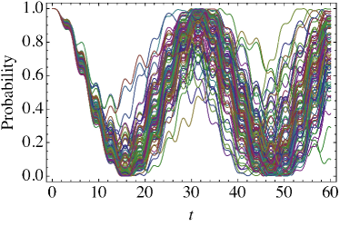
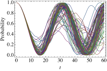
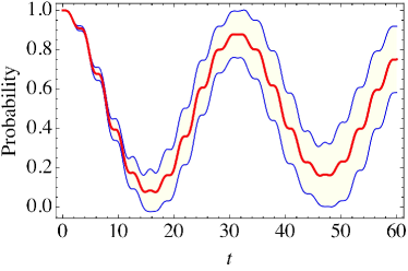
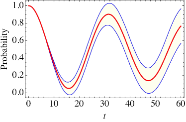
Figure 1: (Color online) Dephasing of on-resonance transitions due to a stochastic field $b_{z}(t)$. (a) 100 stochastic realizations of the probability $P_{b}(t)=|\psi_{b}(t)|^{2}$ versus time for the on-resonance case, for $\delta=1.0$, $\omega=1.0$ and $\Omega=0.2$ in the presence of a stochastic magnetic field along the $z$ direction with volatility $w_{0}=0.1$. (b) 100 stochastic realizations of the rotating wave approximation for the probability $P_{b}(t)$ versus time for the on-resonance case, for $\Delta=0$, $\omega=1.0$ and $\Omega=0.2$ in the presence of a stochastic magnetic field along the $z$ direction with volatility $w_{0}=0.1$. (c) Average probability $\overline{P_{b}(t)}=\overline{\psi_{b}^{*}(t)\psi_{b}(t)}$ and the average plus and minus standard deviation of the probability versus time for $\delta=1.0$, $\omega=1.0$ and $\Omega=0.2$ and a stochastic field in the $z$ direction with volatility $w_{0}=0.1$. (d) Average rotating wave approximation probability $\overline{P_{b}(t)}$ and the average plus and minus standard deviation of the probability versus time for $\Delta=0$, $\omega=1.0$ and$\Omega=0.2$ and a stochastic field in the $z$ direction with volatility $w_{0}=0.1$. For comparison, the insets in (c) and (d) show the results without any noise.

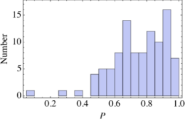
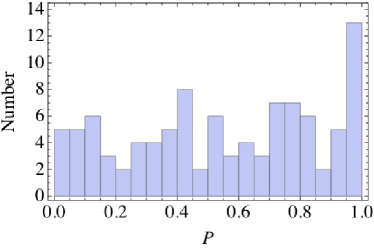
Figure 2: (Color online) (a) Histogram with 100 paths (realizations) of the probability $P_{b}(t)$ in the presence of a stochastic magnetic field along the $z$ direction at the final computed time, $t=60$ shown in Figs. 1(a) and (c). (b) Histogram with 100 paths (realizations) of the probability $P_{b}(t)$ in the presence of an isotropic stochastic magnetic field at the final computed time, $t=60$ to be shown in Fig. 3(a).

III.2 Decoherence due to Isotropic White Noise

Figure 3(a) shows the average probability $\overline{P_{b}(t)}=\overline{\psi_{b}^{*}(t)\psi_{b}(t)}$, and the average plus and minus the standard deviation of the probability calculated using Eq. (13) in the form

$${\dot{\psi}}=\left(-i\,{\cal H}-\frac{3w_{0}^{2}}{2}{\bf 1}\right)\psi+w_{0}\sum_{i}\xi_{i}(t)\sigma_{i}\,\psi,$$ (18)

where the white noise $\xi_{i}(t)$ satisfy $\overline{\xi_{i}(t)}=0$ and $\overline{\xi_{i}(t)\xi_{j}(t^{\prime})}=\delta_{ij}\,\delta(t-t^{\prime})$, with the volatilities $w_{i,0}\equiv w_{0}=0.1$ for $i=1,2,3$. Figure 2(b) shows the histogram of the probability $P_{b}(t)$ at the final computed time, $t=60$, for the case shown in Fig. 3(a).

The RWA (i.e., the transformation to the rotating frame) for the Schrödinger equation in Eq. (18) [or (13)] must be carried out with care because the unitary transformation matrix in Eq. (7) does not commute with the $\sigma_{x}$ and $\sigma_{y}$ stochastic terms in (18). The transformation of the Gaussian white noise Hamiltonian in (18) gives

$$\breve{\cal H}_{\mathrm{st}}(t)={\cal U}^{\dagger}(t)\,[w_{0}{\bm{\xi}}\cdot{\bm{\sigma}}]\,{\cal U}(t)=w_{0}\begin{pmatrix}\xi_{z}&i\,e^{-i\omega t}(\xi_{x}-i\xi_{y})\\ -i\,e^{i\omega t}(\xi_{x}+i\xi_{y})&-\xi_{z}\end{pmatrix},$$ (19)

where ${\cal U}(t)$ is given in Eq. (7), and the SLSDE RWA for Gaussian white noise becomes

$${\dot{\psi}}=-i\,\left({\cal H}_{\mathrm{RWA}}-\frac{3w_{0}^{2}}{2}{\bf 1}+\breve{\cal H}_{\mathrm{st}}(t)\right)\psi.$$ (20)

Figure 3(b) shows the average probability $\overline{P_{b}(t)}$, and the average plus/minus the standard deviation of the probability, calculated using Eq. (20). Figure 3(c) shows the results of using $i{\dot{\psi}}=\left({\cal H}_{\mathrm{RWA}}-\frac{3w_{0}^{2}}{2}{\bf 1}+{\cal H}_{\mathrm{st}}(t)\right)\psi$, which neglects the fact that the RWA transformation and the transverse stochastic Hamiltonian do not commute. There is little difference between the results in Figs. 3(b) and (c), which is not surprising, given that the time dependence of the harmonic function $e^{i\omega t}$, i.e., $\omega^{-1}$, is slow compared to the correlation time $\tau_{\mathrm{corr}}$ of white noise, which is effectively zero (i.e., infinitesimal). A significant difference will occur only if $\omega\tau_{\mathrm{corr}}\gtrapprox 1$. Only for noise with a correlation time $\tau_{\mathrm{corr}}$ comparable to $\omega^{-1}$ or larger are large differences are expected. In Sec. V we discuss the case of an Ornstein–Uhlenbeck process with mean reversion rates comparable to the frequency $\omega$; for such cases, we expect a substantial difference between the results of taking the non-commutation into account or not. Figures 4(a)-(c) show the off-resonance case, $\delta=1.2$, $\omega=1.0$, $\Omega=0.2$. Again, here there is very little difference between the results in Figs. 4(b) and (c), for the same reasons just discussed.

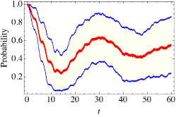
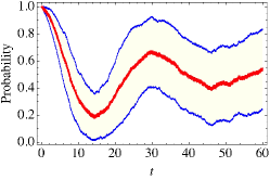
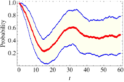
Figure 3: (Color online) Decoherence and dephasing of on-resonance transitions with isotropic white noise. (a) Average probability $\overline{P_{b}(t)}=\overline{\psi_{b}^{*}(t)\psi_{b}(t)}$ and the standard deviation of the probability versus time for $\delta=1.0$, $\omega=1.0$, $\Omega=0.2$ and volatilities $w_{0,1}=w_{0,2}=w_{0,3}=0.1$. (b) Same as (a) (i.e., $\Delta=0$), except calculated using the RWA. (c) Same as (b), except that the non-commutativity of the RWA transformation and the transverse stochastic Hamiltonian not properly accounted for.

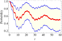
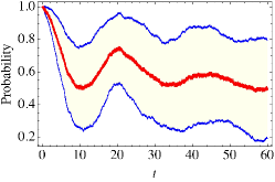
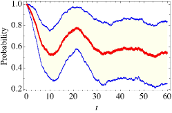
Figure 4: (Color online) Decoherence and dephasing of off-resonance transitions. (a) Average probability $\overline{P_{b}(t)}=\overline{\psi_{b}^{*}(t)\psi_{b}(t)}$ versus time for $\delta=1.2$, $\omega=1.0$, $\Omega=0.2$ and volatilities $w_{0,1}=w_{0,2}=w_{0,3}=0.1$. (b) Same as (a) (i.e., $\Delta=0.2$), except calculated using the RWA. (c) Same as (b), except that the non-commutativity of the RWA transformation and the transverse stochastic Hamiltonian terms is not properly accounted for.

IV Master (Liouville–von Neumann) Equation Results

As already mentioned, white noise gives average results that are identical to those obtained with a Markovian Liouville-von Neumann density matrix equation having Lindblad terms. For the isotropic white noise case in Eq. (18) the corresponding density matrix equation is

$${\dot{\rho}}=-i[{\cal H}(t),\rho(t)]+w_{0}^{2}\left(3\rho(t)-\sum_{i}\sigma_{i}\,\rho(t)\,\sigma_{i}\right).$$ (21)

Figure 5 shows the results of such density matrix calculations. Figure 5(a) is for the on-resonance dephasing case with Lindblad operator $\sigma_{z}$ [this case of white noise only in the $z$ component of the magnetic field, see Eq. (16), gives the master equation, ${\dot{\rho}}=-i[{\cal H}(t),\rho(t)]+w_{0}^{2}(\rho(t)-\sigma_{z}\,\rho(t)\,\sigma_{z})$], Fig. 5(b) is for the on-resonance isotropic white noise case, and Fig. 5(c) is for the off-resonance case with $\Delta=1.2$, $\omega=1.0$. In particular, $\rho_{bb}(t)$ using the density matrix (master equation) treatment is identical, to within numerical accuracy, to the average probabilities $\overline{P_{b}(t)}$ computed with the stochastic differential equation approach. However, the Liouville-von Neumann density matrix approach cannot easily determine the distribution ${\cal D}[P_{b}(t)]$ of the probability $P_{b}(t)$ (to do so would require calculating $P_{b}^{m}(t)$ for all poowers $m$), which can be directly obtained using the stochastic equation approach.

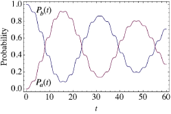
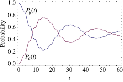
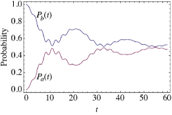
Figure 5: (Color online) Master (Liouville-von Neumann density matrix) equation calculations of dephasing and decoherence. (a) Dephasing of the probability $\rho_{bb}(t)$ versus time for the on-resonance case, $\delta=1.0$, $\omega=1.0$, $\Omega=0.2$, and white noise in the $z$ component of the magnetic field with volatility $w_{0}=0.1$. (b) Decoherence and dephasing of the probability $\rho_{bb}(t)$ versus time for $\delta=1.0$, $\omega=1.0$, $\Omega=0.2$, and isotropic white noise with volatilities $w_{0,1}=w_{0,2}=w_{0,3}=0.1$. (c) Same as for (b), except for the off-resonance case with $\delta=1.2$, $\omega=1.0$.

Now, consider the RWA. The analytic solution to Eq. (21) (isotropic Gaussian white noise), using the RWA Hamiltonian ${\cal H}_{\mathrm{RWA}}(t)$ instead of ${\cal H}(t)$, is given by

$$\rho_{bb}(t)=\frac{1}{2}\left\{1+\frac{e^{-4w_{0}t}[\Delta^{2}+\Omega^{2}\cos(\Omega_{g}t)]}{4\Omega_{g}^{2}}\right\},$$

$$\rho_{ba}(t)=\frac{e^{-4w_{0}t}\Omega\left[\Delta-\Delta\cos(\Omega_{g}t)+i\Omega_{g}\sin(\Omega_{g}t)\right]}{4\Omega_{g}^{2}},$$

$$\rho_{ab}(t)=\rho_{ba}^{*}(t),$$

$$\rho_{aa}(t)=\frac{1}{2}\left\{1-\frac{e^{-4w_{0}t}[\Delta^{2}+\Omega^{2}\cos(\Omega_{g}t)]}{4\Omega_{g}^{2}}\right\}.$$ (22)

where $\Omega_{g}\equiv\sqrt{\Omega^{2}+\Delta^{2}}$. Figure 6(a) plots the probabilities $\rho_{bb}(t)$ and $\rho_{aa}(t)$ and the purity ${\mathrm{Tr}}[\rho^{2}(t)]$ versus time for the on-resonance case. As $t\to\infty$, the purity goes to 1/2 and the density matrix decays to the democratic state $\frac{1}{2}\binom{1\,0}{0\,1}$. Figure 6(b) plots the coherence $\rho_{ba}(t)$ versus time; it has only an imaginary component and it decays to zero as $t\to\infty$. The decay rate of the populations and the coherence is $4w_{0}$, as is evident from the expressions in Eq. (22)]. Properly accounting for the non-commutativity of the RWA transformation and the stochastic Hamiltonian, i.e., using the stochastic Hamiltonian in Eq. (19), does not significantly affect the numerical results for white Gaussian noise. The full RWA probabilities, including non-commutativity effects, are indistinguishable by eye from the results shown in Fig. 6. The full RWA coherence ${\mathrm{Im}}[\rho_{ba}(t)]$ is also indistinguishable by eye, and the ${\mathrm{Re}}[\rho_{ba}(t)]$ is more than an order of magnitude smaller than the imaginary part.

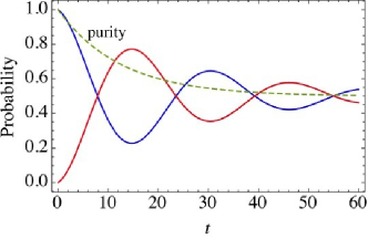
Figure 6: (Color online) Analytic results obtained using Eq. (22) for the density matrix for isotropic white noise in the on-resonance case with $\delta=1.0$, $\omega=1.0$, $\Omega=0.2$, and $w_{0}\equiv w_{0,1}=w_{0,2}=w_{0,3}=0.1$. (a) Density matrix elements $\rho_{bb}(t)$ and $\rho_{aa}(t)$, and the purity ${\mathrm{Tr}}[\rho^{2}(t)]$ (dashed green curve) versus time. Compare with the non-RWA results in Fig. 5(b). (b) Off-diagonal density matrix $\rho_{ba}(t)$ versus time. The real part of $\rho_{ba}(t)$ vanishes for the on-resonance case.

V Ornstein–Uhlenbeck Process

Many kinds of stochastic processes have been studied. In order to see significant effects due to the non-commutativity of the RWA transformation and stochastic part of the total Hamiltonian $\tilde{H}(t)={\cal H}(t)+{\cal H}_{\mathrm{st}}(t)$, we need a stochastic process with a correlation time $\tau_{\mathrm{corr}}$ comparable to or greater than the timescale of the driven two level system $\omega^{-1}$. A well-known finite-correlation-time stochastic process is the Ornstein–Uhlenbeck process, which is an example of Gaussian colored noise, which is a generalization of Brownian motion OU_30 . The mean and the autocorrelation function of an Ornstein–Uhlenbeck process are

$$\overline{{\cal O}_{i}(t)}={\cal O}_{0,i}\,e^{-\vartheta_{i}t}+\mu_{i}(1-e^{-\vartheta_{i}t}),\quad\overline{{\cal O}_{i}(t)\,{\cal O}_{j}(t^{\prime})}=\delta_{ij}\frac{w_{0,i}^{2}}{2\vartheta_{i}}e^{-\vartheta_{i}(t+t^{\prime})}[e^{\vartheta_{i}\,{\mathrm{min}}(t,t^{\prime})}-1].$$ (23)

Here $\vartheta_{i}$ is the mean reversion rate of the Ornstein–Uhlenbeck process ${\cal O}_{i}(t)$, which is the inverse of the noise correlation time, $\tau_{\mathrm{corr},i}=\vartheta_{i}^{-1}$, $w_{0,i}$ is its volatility, and $\mu_{i}$ is the mean of the process, which we take to vanish, $\mu_{i}=0$; we also take ${\cal O}_{0,i}=0$. The stochastic differential equations that we solve are,

$$d\psi(t)=\left[-i\,{\cal H}\psi+\sum_{i}{\cal O}_{i}(t)\sigma_{i}\psi(t)\right]\,dt,$$ (24a)

$$d{\cal O}_{i}(t)=\vartheta_{i}\left[\mu_{i}-{\cal O}_{i}(t)\right]\,dt+w_{0,i}\,dw_{i}(t).$$ (24b)

For determining the effects of the non-commutativity of the RWA transformation and stochastic terms in the total Hamiltonian, it is sufficient to use only the term $i=x$ in the sum in Eq. (24a). Doing so simplifies the convergence of the calculation relative to using isotropic Ornstein–Uhlenbeck noise.

Figure 7 shows the calculated average probability $\overline{P_{b}(t)}$ versus time and the average plus and minus the standard deviation of the probability calculated using Eq. (24) for Ornstein–Uhlenbeck noise in the $x$ component of the magnetic field for the on-resonance case, $\delta=1.0$, $\omega=1.0$, $\Omega=0.2$. Figure 7(b) is calculated using the RWA, and for comparison purposes only, (c) shows the results using a RWA but ignoring the non-commutativity of the RWA transformation and the transverse stochastic Hamiltonian term, i.e., ignoring the factors $e^{\pm i\omega t}$ in the off-diagonal elements of the Hamiltonian

$$\tilde{\cal H}_{\mathrm{RWA}}(t)={\cal H}_{\mathrm{RWA}}+{\cal H}_{\mathrm{st,RWA}}(t)=\begin{pmatrix}-\Delta&\Omega\\ \Omega&0\end{pmatrix}+\begin{pmatrix}b_{z}(t)&i\,e^{-i\omega t}[b_{x}(t)-ib_{y}(t)]\\ -i\,e^{i\omega t}[b_{x}(t)+ib_{y}(t)]&-b_{z}(t)\end{pmatrix}.$$ (25)

The oscillating factors $e^{\pm i\omega t}$ in the off-diagonal terms can be ignored if $\omega\tau_{\mathrm{corr}}\ll 1$, but not otherwise. In Fig. 7 we used $\omega\tau_{\mathrm{corr}}=1$, so we expect that the non-commutativity cannot be ignored, and we took noise only in the $x$-component of the magnetic field. The calculations in Fig. 7 were hard to converge with respect to the time-step used, hence we only continued them out to a final time of $t=20$. Note that the standard deviation in Fig. 7(c) is significantly reduced relative to (a) and (b), and the width becomes very close to zero at $t=15.5$ where the average probability goes to zero, unlike the results in (a) and (b). Clearly, the results of ignoring the non-commutativity of the RWA transformation and the transverse stochastic Hamiltonian are very different from the RWA taking the non-commutativity into account. The minimum of the probability in (c) is shifted to somewhat smaller time and is much closer to zero probability than in (b); moreover the standard deviation in (c) is much smaller than in (b). We also expect a difference between taking and not taking the non-commutativity into account in a master equation approach. The master equation for OU noise could in principle be determined using cumulant generating functional methods and requires calculation of time-ordered exponential functions Kubo_cumulants but this is a difficult task. Figure 8 shows $\overline{P_{b}(t)}$ for isotropic Ornstein–Uhlenbeck noise for the off-resonance case, $\Delta=0.2$. Here, the differences between (b) and (c) are small. No difference between (b) and (c) results due to the $z$-component of the noise field, whose noise Hamiltonian commutes with the RWA transformation; moreover, there is some compensation which takes place between the $x$ and $y$ components.

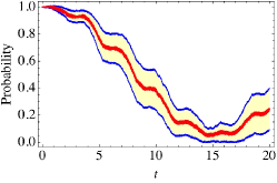
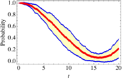
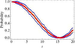
Figure 7: (Color online) Ornstein-Olhenbeck noise and on-resonance radiation, highlighting the effects of the non-commutativity of the RWA transformation and the transverse stochastic Hamiltonian. (a) Probability $\overline{P_{b}(t)}$ versus time for the on-resonance case, $\delta=1.0$, $\omega=1.0$ (so $\Delta=0$), $\Omega=0.2$, and Ornstein-Olhenbeck noise in the $x$ component of the magnetic field, with volatility $w_{0,x}=0.1$ and mean reversion rate $\vartheta_{x}=1$ (so $\omega\tau_{\mathrm{corr}}=1$). (b) Same as (a) except calculated using the RWA. (c) Same as (b), except that the non-commutativity of the RWA transformation and the transverse stochastic Hamiltonian term is not properly accounted for.

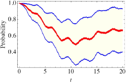
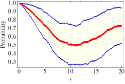
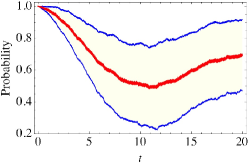
Figure 8: (Color online) Isotropic Ornstein-Olhenbeck noise and off-resonance radiation, $\Delta=0.2$. (a) Probability $\overline{P_{b}(t)}$ versus time for the off-resonance case, $\delta=1.2$, $\omega=1.0$ (so $\Delta=0.02$), $\Omega=0.2$, and isotropic Ornstein-Olhenbeck noise in the magnetic field, with volatilities $w_{0,x}=w_{0,y}=w_{0,z}=0.1$ and mean reversion rate $\vartheta_{x}=1$ (so $\omega\tau_{\mathrm{corr}}=1$). (b) Same as (a) except calculated using the RWA. (c) Same as (b), except that the non-commutativity of the RWA transformation and the transverse stochastic Hamiltonian term is not properly accounted for.

VI Summary and conclusions

Much of our experience with quantum dynamics comes from applying it to two-level systems driven by an electromagnetic field. But such systems are never truly isolated, and their interaction with their environment affect their mysterious quantum properties, i.e., their quantum coherence. Such interaction is at the heart of the fundamental limitations of quantum metrology and quantum information processing. Using the Schrödinger-Langevin stochastic differential equation (SLSDE) formalism, we studied the dynamics of a two-level quantum system driven by single frequency electromagnetic field, with and without making the rotating wave approximation (RWA). If the transformation to the rotating frame does not commute with the stochastic Hamiltonian, i.e., if the stochastic field has nonvanishing components in the transverse direction, the RWA modifies the stochastic terms in the Hamiltonian. The decay terms in a master equation (i.e., the Liouville–von Neumann density matrix equation) will also be affected. We found that for Gaussian white noise, the master equation for the density matrix is easily derived from the SLSE, with and without the RWA. For the RWA, both the SSLE and the derived master equation have Lindblad terms with coefficients that are time-dependent (i.e., the master equation is time-local Fleming_12b ) when the non-commutation of the RWA transformation and the noise Hamiltonian is properly accounted for. But since $\omega\tau_{\mathrm{corr}}$ effectively vanishes for white Gaussian noise, it is not necessary to take the non-commutation into account, independent of the strength of the noise ($w_{0}$), and we obtain an analytic expression for the density matrix of the system, Eq. (22), which fully describes the dynamics of the two-level system in the presence of the noise. On the other hand, for the non-Markovian Ornstein–Uhlenbeck noise case, the RWA dynamics must be calculated taking the non-commutation of the RWA transformation and the noise Hamiltonian into account when $\omega\tau_{\mathrm{corr}}\gtrapprox 1$.

Decoherence and dephasing of two-level systems can be probed by measuring the population decay ($T_{1}$) and the transverse relaxation time ($T_{2}$) in magnetic resonance studies Jarmola_12 ; Kehayias_14 . One well-studied physical system in which such studies have been carried out is the negatively-charged nitrogen-vacancy (NV) color center in diamond. An NV center consists of a substitutional nitrogen atom adjacent to a missing carbon atom within the diamond crystal lattice Doherty_13 . The negatively charged NV center has a discrete electronic energy level structure and a ground electronic state of symmetry ${}^{3}A_{2}$, where this state designation refers to an irreducible representation of the $C_{3v}$ group. The three electronic magnetic sub-levels of the triplet ground state are $|S,M\rangle$, where $S=1$ and $M=0,\pm 1$, with the $z$ axis (quantization axis) taken along the NV axis. The three $S=1$ ground state levels are split by a spin-spin (crystal field) interaction that raises the energy of the $|1,\pm 1\rangle$ states with respect to the $|1,0\rangle$ state by ${\cal D}=2.87$ GHz. The NV system can behave like a two-level system if one of the three states is not allowed to be populated. The main sources of decoherence are from the paramagnetic impurity spin bath, which dominates at high nitrogen concentration, and interactions with the spin 1/2 ¹³C nuclei Balas_09 ; Taylor_08 . Population decay, $T_{1}$, is dominated by Raman-type interactions with lattice phonons at high temperature (room temperature and above), Orbach-type interaction with local phonons at lower temperatures Jarmola_12 ; Takahashi_08 ; Redman_91 , and at temperatures below about 100 K, density-dependent cross-relaxation effects between NV centers and between NVs and other impurities. At these low temperatures, the resulting $T_{1}$ can be dramatically tuned using an external magnetic field Jarmola_12 . For dilute samples, the contribution of NV–NV dipolar interactions to the magnetic resonance broadening can be approximated by assuming that each NV center couples to neighboring NV centers, to substitutional nitrogen (P1) centers, which have a spin of 1/2, and with ¹³C nuclei, which have a nuclear spin of 1/2 and a natural abundance of about 1%. Dipolar coupling with other NV centers leads to a spin-relaxation contribution on the order of $\gamma_{\mathrm{NV}}\approx(g_{s}\mu_{B})^{2}n_{\mathrm{NV}}$, where $n_{\mathrm{NV}}$ is the NV concentration Taylor_08 ; Acosta_09 . For [NV] = 15 ppm, this corresponds to $\gamma_{\mathrm{NV}}\approx 10^{6}$ s${}^{-1}\approx\gamma_{C}$, where $\gamma_{C}$ is the spin relaxation rate to to the ¹³C nuclei. Since the dynamics of the ¹³C nuclear spin is slow, it can be modeled, to good approximation, as quasi-static Guassian noise. Since the spin dynamics of the NV centers and PI centers in diamond are fast, the contribution of NV–NV and NV–P1 interactions can be modeled, to good approximation, as Gaussian white noise. As demonstrated in Ref. Kehayias_14 , CW hole-burning and lock-in detection can be used to eliminate the linewidth contribution from slowly fluctuating ¹³C nuclei while rapidly fluctuating magnetic fields from nearby substitutional nitrogen (P1) centers and NV centers continue to contribute to a reduced linewidth. Hence, by adjusting the external magnetic field strength and the concentrations of NV centers, P1 centers and ¹³C, the volatilities $w_{0}$, the stochastic magnetic field correlation times $\tau_{\mathrm{corr}}$ and the detuning from resonance $\Delta$ can be modified. If only two of the three triplet ground state levels $|S,M\rangle$ are populated, the methods developed in this manuscript can be applied directly; if all three levels are populated, it is straightforward to generalize the spin 1/2 treatment here to $S=1$. In either case, the conclusions we obtained are quite general and are expected to apply to the NV diamond system. One would, of course need to know the correlation times and the strength of the noises affecting the NV centers. Specifically, if the correlation time $\tau_{\mathrm{corr}}$ of the noise (of the bath coupled to the system) is of order of the frequency of the electromagnetic field $\omega$ that couples the levels, the non-commutativity of the RWA transformation and the noise Hamiltonian must be taken into account, even when the criteria for validity of the RWA for the system are satisfied. For diamond NV centers, the resonant frequency $\omega$ for transitions from $M=0$ to $M=\pm 1$ is of order GHz (with no external magnetic field, it is 2.87 GHz), so for $\omega\tau_{\mathrm{corr}}\approx 1$, $\tau_{\mathrm{corr}}$ must be of order milliseconds. When $\omega\tau_{\mathrm{corr}}\ll 1$, the non-commutativity need not be taken into account.

Acknowledgement. This work was supported in part by grants from the Israel Science Foundation (Grant No. 295/2011). I am grateful to Professors Yshai Avishai and Dmitry Budker for valuable discussions.

References

- (1) I. L. Aleiner, B. L. Altshuler, and Y. M. Galperin “Experimental tests for the relevance of two-level systems for electron dephasing”, Phys. Rev. B63, 201401(R) (2001).
- (2) F. Dolde, H. Fedder, M.W. Doherty, T. Nöbauer, F. Rempp, G. Balasubramanian, T. Wolf, F. Reinhard, L. C. L. Hollenberg, F. Jelezko, and J. Wrachtrup, “Electric-field sensing using single diamond spins”, Nat. Phys. 7, 459 (2011); V. M. Acosta, K. Jensen, C. Santori D. Budker and R. G. Beausoleil, “Electromagnetically Induced Transparency in a Diamond Spin Ensemble Enables All-Optical Electromagnetic Field Sensing”, Phys. Rev. Lett. 110, 213605 (2013); J. Zhou, P. Huang, Q. Zhang, Z. Wang, T. Tan, X. Xu, F. Shi, X. Rong, S. Ashhab, and J. Du, “Observation of Time-domain Rabi Oscillations in the Landau–Zener Regime with a Single Electronic Spin”, arXiv:1305.0157.
- (3) D. E. Chang, Jun Ye, and M. D. Lukin, “Controlling dipole-dipole frequency shifts in a lattice-based optical atomic clock”, Phys. Rev. A69, 023810 (2004).
- (4) A. Steane, “Quantum Computing”, Rep. Prog. Phys. 61, 117 (1998); J. I. Cirac, P. Zoller, “New frontiers in quantum information with atoms and ions”, Physics Today 57, 38, March 2004.
- (5) H.-P. Breuer and F. Petruccione, Theory of Open Quantum Systems, (Oxford University Press, Oxford, 2002); U, Weiss, Quantum Dissipative Systems, (World Scientific, Singapore, 1999); M. Schlosshauer, Decoherence and the Quantum-to-Classical Transition, (Springer, Berlin, 2007).
- (6) G. Lindblad, “On the generators of quantum dynamical semigroups”, Commun. Math. Phys. 48, 119 (1976); A. Kossakowski, V. Gorini, E.C.G. Sudarshan, “Completely positive dynamical semigroups of -level systems”, J. Math. Phys. 17, 821 (1976).
- (7) N. G. Van Kampen, Stochastic Processes in Physics and Chemistry, (Elsevier, Amsterdam, 1997). See particularly Sec. 7.5, Schrödinger-Langevin and quantum master equations.
- (8) C. W. Gardiner, Handbook of Stochastic Methods for Physics, Chemistry and the Natural Sciences, Third Ed., (Springer, Berlin, 2004).
- (9) C. H. Fleming and B. L. Hu, “Non-Markovian dynamics of open quantum systems: Stochastic equations and their perturbative solutions”, Annals of Physics 327, 1238 (2012).
- (10) P. Szańkowski, M. Trippenbach and Y. B. Band, “Spin Decoherence due to Fluctuating Fields”, Phys. Rev. E87, 052112 (2013); Y. B. Band, “Electric Dipole Moment in a Stochastic Electric Field”, Phys. Rev. E88, 022127 (2013); Y. B. Band and Y. Ben-Shimol, “Molecules with an Induced Dipole Moment in a Stochastic Electric Field”, Phys. Rev. E88, 042149 (2013); Y. Avishai, Y. B. Band, “The Landau-Zener Problem with Decay and with Dephasing”, arXiv:1311.3919 [quant-ph].
- (11) J. Rice, Mathematical Statistics and Data Analysis, Second Ed., (Duxbury Press, 1995); R. B. Ash, Basic Probability Theory (Dover, NY, 2008).
- (12) The Hamiltonian in Eq. (1) is often termed semiclassical because the electromagnetic field is treated classically, rather than using a second-quantized radiation field.
- (13) L. Accardi and Y. Lu, “The weak-coupling limit without rotating wave approximation”, Annales De L’Institut Henri Poincare-Physique Theorique 54, 435-458 (1991).
- (14) A. A. Villaeys, A. Boeglin and S. H. Lin, “Dynamics of stochastic-systems in nonlinear optics. 1. General formalism”, Physical Review A 44, 4660-4670 (1991).
- (15) M. Grifoni, M. Sassetti, P. Hanggi, and U. Weiss, “Cooperative effects in the nonlinearly driven spin-boson system”, Phys. Rev. E 52, 3596-3607 (1995).
- (16) P. Stenius, A. Imamoglu, “Stochastic wavefunction methods beyond the Born-Markov and rotating-wave”, Quantum and Semiclassical Optics 8, 283-295 (1996).
- (17) S. V. Prants, L.E. Kon’kov, “Parametric instability and Hamiltonian chaos in cavity semiclassical”, J. Exp. Theor. Physics 88, 406-414 (1999).
- (18) C. Q. Cao, C. G. Yu, H. Cao, “Spontaneous emission of an excited two-level atom without both”, European Physical Journal D 23, 279-284 (2003).
- (19) T. Yu, “Non-Markovian quantum trajectories versus master equations”, Phys. Rev. A 69 (2004).
- (20) A. Ishizaki, Y. Tanimura, “Multidimensional vibrational spectroscopy for tunneling processes in a dissipative environment”, J. Chem. Phys. 123, 014503 (2005).
- (21) A. Ishizaki and Y. Tanimura, “Modeling vibrational dephasing and energy relaxation of intramolecular anharmonic modes for multidimensional infrared spectroscopies”, J. Chem. Phys. 125, 084501 (2006).
- (22) R. Schmidt, A. Negretti, J. Ankerhold, T. Calarco, and J. T. Stockburger, “Optimal Control of Open Quantum Systems: Cooperative Effects of Driving”, Physical Review Letters 107, 130404 (2011).
- (23) A. C. Doherty, A. Szorkovszky, G. I. Harris, and W. P. Bowen, “The quantum trajectory approach to quantum feedback control of an oscillator revisited”, Philosophical Transactions of the Royal Society A–Mathematical Physical 370, 5338-5353 (2012).
- (24) C. H. Fleming, N. I. Cummings, C. Anastopoulos, and B. L. Hu, “The rotating-wave approximation: consistency and applicability from an open quantum system analysis”, J. Phys. A: Math. Theor. 43, 405304 (2010).
- (25) C. H. Fleming, N. I. Cummings, C. Anastopoulos, and B. L. Hu, “Non-Markovian dynamics and entanglement of two-level atoms in a common field”, J. of Physics A-Mathematical and Theoretical 45, 065301 (2012).
- (26) M. A. Desposito, S. M. Gatica and E. S. Hernandez, “Asymptotic regime of quantal stochastic and dissipative motion”, Phys. Rev. A 46, 3234-3242 (1992).
- (27) F. Bloch and A. Siegert, Phys. Rev. 57, 522 (1940).
- (28) Y. B. Band and Y. Avishai, Quantum Mechanics, with Applications to Nanotechnology and Quantum Information Science, (Academic Press – Elsevier, 2013), Sec. 6.1.4.
- (29) K. Molmer, Y. Castin and J. Dalibard, “Monte Carlo wave-function method in quantum optics”, J. Opt. Soc. Am B10, 524 (1993).
- (30) P. E. Kloeden and E. Platen, Numerical Solution of Stochastic Differential Equations, (Springer, Berlin, 2011).
- (31) P. E. Kloeden, E. Platen and H. Schurz, Numerical Solutions of Stochastic Differential Equations Through Computer Experiments, (Springer, Berlin, 2003).
- (32) http://reference.wolfram.com/mathematica/ref/ItoProcess.html.
- (33) G. E. Uhlenbeck and L. S. Ornstein, “On the theory of Brownian Motion”, Phys. Rev. 36, 823 (1930).
- (34) P. Ao and J. Rammer, “Influence of Dissipation on the Landau-Zener Transition”, Phys. Rev. Lett. 62, 3004 (1989); “Quantum dynamics of a two-state system in a dissipative environment”, Phys. Rev. B43, 5397 (1991).
- (35) E. Shimshoni and Y. Gefen, “Onset of dissipation in Zener dynamics: Relaxation versus dephasing”, Ann. Phys. (NY) 210, 16 (1991).
- (36) E. Shimshoni and A. Stern, “Dephasing of interference in Landau-Zener transitions”, Phys. Rev. B47, 9523 (1993).
- (37) V. L. Pokrovsky and D. Sun, “Fast quantum noise in the Landau-Zener transition””, Phys. Rev. B76, 024310 (2007).
- (38) J. E. Avron, M. Fraas, G. M. Graf and P. Grech, “Landau-Zener Tunneling for Dephasing Lindblad Evolutions”, Commun. Math. Phys. 305, 633 (2011).
- (39) One might be able to use the methods introduced in R. Kubo, “Generalized Cumulant Expansion Method”, J. Phys. Jap. 17, 1100 (1962); R. Kubo, “Stochastic Liouville Equations”, J. Math. Phys. 4, 174 (1963).
- (40) A. Jarmola, V. M. Acosta, K. Jensen, S. Chemerisov, and D. Budker “Temperature- and Magnetic-Field-Dependent Longitudinal Spin Relaxation in Nitrogen-Vacancy Ensembles in Diamond” Phys. Rev. Lett. 108, 197601 (2012).
- (41) P. Kehayias et al., “Microwave saturation spectroscopy of nitrogen-vacancy ensembles in diamond”, arXiv:1403.2119.
- (42) M. W. Doherty et al., “The nitrogen-vacancy colour centre in diamond”, Phys. Reports 528, 1 (2013).
- (43) G. Balasubramanian et al., “Ultralong spin coherence time in isotopically engineered diamond”, Nat. Mater. 8, 383 (2009).
- (44) J. M. Taylor et al., “High-sensitivity diamond magnetometer with nanoscale resolution”, Nat. Phys. 4, 810 (2008).
- (45) S. Takahashi, R. Hanson, J. van Tol, M. S. Sherwin, and D. D. Awschalom, “Quenching Spin Decoherence in Diamond through Spin Bath Polarization”, Phys. Rev. Lett. 101, 47601 (2008).
- (46) D. A. Redman, S. Brown, R. H. Sands, and S. C. Rand, “Spin dynamics and electronic states of NV centers in diamond by EPR and four-wave-mixing spectroscopy”, Phys. Rev. Lett. 67, 3420 (1991).
- (47) V. M. Acosta et al., “Diamonds with a high density of nitrogen vacancy centers for magnetometry applications”, Phys. Rev. B80, 115202 (2009).