MMT Hypervelocity Star Survey III: A Complete Survey of Faint B-type Stars in the Northern Milky Way Halo

Abstract

We describe our completed spectroscopic survey for unbound hypervelocity stars (HVSs) ejected from the Milky Way. Three new discoveries bring the total number of unbound HVSs to 21. We place new constraints on the nature of HVSs and on their distances using moderate resolution MMT spectroscopy. Half of the HVSs are fast rotators; they are certain 2.5 - 4 $M_{\odot}$ main sequence stars at 50 - 120 kpc distances. Correcting for stellar lifetime, our survey implies that unbound 2.5 - 4 $M_{\odot}$ stars are ejected from the Milky Way at a rate of $1.5\times 10^{-6}$ yr^-1. The observed HVSs are likely ejected continuously over the past 200 Myr and do not share a common flight time. The anisotropic spatial distribution of HVSs on the sky remains puzzling. Southern hemisphere surveys like SkyMapper will soon allow us to map the all-sky distribution of HVSs. Future proper motion measurements with Hubble Space Telescope and Gaia will provide strong constraints on origin. All existing observations are consistent with HVS ejections from encounters with the massive black hole in the Galactic center.

1. INTRODUCTION

HVSs are unbound stars escaping the Milky Way. Hills (1988) first predicted their existence as a consequence of the massive black hole (MBH) in the Galactic center. Present-day observations provide compelling evidence for a $4\times 10^{6}$ $M_{\odot}$ central MBH, surrounded by an immense crowd of stars (Gillessen et al., 2009; Do et al., 2013). Theorists estimate that three-body interactions with this MBH will unbind stars from the Galaxy at a rate of $\sim$10^-4 yr^-1 (Hills, 1988; Yu & Tremaine, 2003; Perets et al., 2007; Zhang et al., 2013). The ejection rate of unbound stars by the central MBH is 100$\times$ larger than the rate expected by competing mechanisms, including unbound runaway ejections from the Galactic disk (Brown et al., 2009a; Perets & Subr, 2012).

Brown et al. (2005) serendipitously discovered the first HVS in the outer stellar halo, a B-type star moving over twice the Galactic escape velocity. This discovery motivated our targeted HVS Survey with the MMT telescope. The HVS Survey has identified at least 16 unbound stars over the past seven years (Brown et al., 2006a, b, 2007b, 2007c, 2009a, 2009b, 2012b). Other observers have found unbound and candidate unbound stars among a range of stellar types (Hirsch et al., 2005; Edelmann et al., 2005; Heber et al., 2008a; Tillich et al., 2009; Irrgang et al., 2010; Tillich et al., 2011; Li et al., 2012). The variety of HVS observations has led to some confusion.

HVSs are rare objects. Of the Milky Way’s $10^{11}$ stars, there should be only 1 HVS within 1 kpc of the Sun for an HVS ejection rate of $10^{-4}$ yr^-1. Thus the vast majority of fast-moving stars near the disk are disk runaways (Bromley et al., 2009), not HVSs ejected by the MBH. Heber et al. (2008a)’s discovery of the first unbound B star ejected from the disk is a case in point. The Milky Way’s stellar halo contains a millionfold more normal stars than HVSs, as demonstrated by the absence of unbound A- and F-type stars in the Sloan Digital Sky Survey (Kollmeier & Gould, 2007; Kollmeier et al., 2009, 2010). In this context, metal poor F-type stars with marginally unbound proper motion velocities are probably halo stars.

The HVS Survey is a clean, well-defined spectroscopic survey of stars with the colors of 2.5 - 4 $M_{\odot}$ stars. These stars should not exist at faint magnitudes in the outer halo unless they were ejected there. The stars we define as HVSs are significantly unbound in radial velocity alone. To date, all follow-up observations show that the HVSs are main sequence B stars at 50 - 100 kpc distances (Fuentes et al., 2006; Przybilla et al., 2008b; López-Morales & Bonanos, 2008; Brown et al., 2012a, 2013a). B-type stars have relatively short lifetimes and must originate from a region with on-going star formation, such as the Galactic disk or Galactic center. For those HVSs with detailed echelle spectroscopy, their stellar ages exceed their flight times from the Galaxy by $\simeq$100 Myr, an observation difficult to reconcile with Galactic disk runaway scenarios involving massive stars (Brown et al., 2012a, 2013a).

Here we describe the completed MMT HVS Survey. In Section we begin 2 by describing our data and the discovery of 3 new HVSs. One of these HVSs is in the south Galactic cap where there are few other HVS discoveries to date. In Section 3 we describe our stellar atmosphere fits to the HVS spectra, and identify rapidly rotating HVSs that are certain main sequence B stars at 50 - 120 kpc distances. In Section 4 we investigate the flight time distribution of HVSs and find that the full sample of HVSs is best described by a continuous distribution. The eleven HVSs clumped around the constellation Leo have flight times equally well described by a burst or a continuous distribution. In Section 5 we predict proper motions for allowable Galactic disk and Galactic center ejection origins, and show that future proper motion measurements with Hubble Space Telescope and Gaia can distinguish between these origins. Finally, in Section 6 we use the completed HVS sample to estimate a $1.5\times 10^{-6}$ yr^-1 ejection rate of unbound 2.5 - 4 $M_{\odot}$ stars from the Milky Way.

2. DATA

2.1. Target Selection

The HVS Survey is a spectroscopic survey of late B-type stars selected by broadband color (Brown et al., 2006a). The final color selection is detailed in Brown et al. (2012b) and we do not repeat it here. Photometry comes from the Sloan Digital Sky Survey (SDSS, Aihara et al., 2011). We correct all photometry for reddening following Schlegel et al. (1998) and exclude any region with high reddening $E(B-V)>0.1$ mag. We also exclude two small end-of-stripe regions with bad colors, and all objects within 2° of M31. The revised list contains 1451 HVS Survey candidates.

The HVS Survey color selection primarily identifies evolved blue horizontal branch (BHB) stars in the stellar halo, but it also identifies some $\simeq$3 $M_{\odot}$ main sequence B stars. BHB stars and $\simeq$3 $M_{\odot}$ main sequence B stars share similar effective temperatures and surface gravities in the color range of the HVS Survey, and both BHB and main sequence B stars are intrinsically luminous objects ($g$-band absolute magnitudes $-1<M_{g}<1$ mag). Because the HVS Survey covers high Galactic latitudes $|b|\gtrsim 30\arcdeg$, the $17<g_{0}<20.25$ magnitude-limited HVS Survey exclusively targets stars in the stellar halo of the Milky Way.

2.2. Spectroscopic Observations and Sample Completeness

We obtain spectra for 269 new HVS Survey candidates. We also obtained repeat observations of previously identified HVSs to validate their nature and radial velocities. New observations were acquired at the 6.5m MMT Observatory in five observing runs between April 2012 and October 2013. All observations were obtained with the Blue Channel Spectrograph (Schmidt et al., 1989) using the 832 line mm^-1 grating and the 1″ slit. This set-up provides a wavelength coverage of 3650 Å – 4500 Å at a spectral resolution of 1.0 Å. We chose exposure times to yield a signal-to-noise ratio (S/N) of 10 to 15 per resolution element in the continuum. All observations were paired with a He-Ne-Ar lamp exposure for accurate wavelength calibration, and were flux-calibrated using blue spectrophotometric standards (Massey et al., 1988).

We have now obtained spectra for 1435 of the 1451 HVS Survey candidates. This count includes 63 objects with spectra taken from SDSS. The HVS Survey completeness is thus 99%. In our sample we find 255 (18%) hydrogen atmosphere white dwarfs, 24 (2%) quasars, and 30 (2%) miscellaneous objects such as metal poor galaxies (Kewley et al., 2007) and B supergiants (Brown et al., 2007a, 2012b). Low-mass white dwarfs are a problematic contaminant: they can appear as velocity outliers because of binary orbital motion (Kilic et al., 2007b). We have thus systematically identified and removed the low mass white dwarfs for study elsewhere (Kilic et al., 2010, 2011, 2012; Brown et al., 2010c, 2012c, 2013b). Our focus here is the cleanly selected sample of 1126 late B-type stars. This complete spectroscopic sample is the basis for the following analysis.

Figure 1.— Distribution of Galactic rest-frame velocity and de-reddened $g$-band magnitude for the 1126 late B-type stars in the HVS Survey. Stars with velocity errors greater than 20 km s^-1 are mostly SDSS measurements. The lower panel plots the velocity histogram emphasizing the tails of the distribution (the histogram peaks at $N_{obs}=104$ in this binning). The significant lack of $v_{rf}<-275$ km s^-1 stars demonstrates that the majority of bound positive velocity outliers have lifetimes less than the orbital turn-around time. Stars with $v_{rf}>400$ km s^-1 are unbound.

2.3. Radial Velocity Distribution

The goal of the HVS Survey is to find velocity outliers. Having completed the HVS Survey, we re-measured the stellar radial velocities from all of our spectra using the latest version of the cross-correlation package RVSAO (Kurtz & Mink, 1998). As in earlier work, we use high S/N spectra of bright late B- and early A-type radial velocity standards (Fekel, 1999) as our cross-correlation templates. The mean radial velocity uncertainty of our measurements is $\pm$10 km s^-1.

For the 63 objects observed by SDSS we adopt the radial velocity reported by the SEGUE Stellar Parameter Pipeline (Allende Prieto et al., 2008; Smolinski et al., 2011). The mean radial velocity uncertainty of the 63 stars observed by SDSS is $\pm$22 km s^-1.

Our primary interest is not heliocentric velocity, but velocity in the Galactic rest frame. To properly interpret the radial velocities of stars in the halo requires that we correct for the local circular velocity and the motion of the Sun with respect to the disk. We have long assumed a circular velocity of 220 km s^-1, but in Brown et al. (2012b) we adopted a circular velocity of 250 km s^-1 on the basis of disk maser proper motions (Reid et al., 2009; McMillan & Binney, 2010). Subsequently, Bovy et al. (2012) measured a circular velocity of 220 km s^-1 on the basis of stellar radial velocities in the inner halo, but a Local Standard of Rest motion 14 km s^-1 larger than previously measured. These different measurements reconcile with each other for a circular velocity of 235 km s^-1 and the Local Standard of Rest motion of Schönrich et al. (2010), which we adopt here. We thus transform the observed heliocentric radial velocities to Galactic rest frame velocities $v_{rf}$ using

$$v_{rf}=v_{helio}+11.1\cos{l}\cos{b}+247.24\sin{l}\cos{b}+7.25\sin{b},$$ (1)

where $l$ and $b$ are Galactic longitude and latitude.

Figure 1 shows the Galactic rest frame velocity distribution of the HVS Survey stars. Each star is drawn with its errorbars; the largest velocity errors come from the SDSS measurements. The lower panel shows the velocity histogram, in 25 km s^-1 bins, emphasizing the tails of the distribution. The HVS Survey contains mostly halo stars; the stars with $|v_{rf}|<300$ km s^-1 have a 109 km s^-1 line-of-sight velocity dispersion that is nearly constant with increasing depth (Brown et al., 2010b; Gnedin et al., 2010).

The HVS Survey also contains some remarkable velocity outliers, stars that are significantly unbound in radial velocity alone. The escape velocity of the Milky Way at 50 kpc is approximately 350 km s^-1 (see Section 4.2). We observe stars traveling up to +700 km s^-1. Because we measure radial velocity, the full space motion of the stars can only be larger.

Notably, the velocity outliers are all moving away from us, consistent with the picture that they were ejected from the Milky Way. The fastest star moving towards us in the HVS Survey has $v_{rf}=-298\pm 10$ km s^-1, consistent with Galactic escape velocity estimates. We re-observed the star previously reported at $-359$ km s^-1, SDSS J115734.45+054645.58; it is $\log{g}$$\simeq$5 white dwarf in a 13.5 hr orbital period binary (Brown et al., 2013b).

Interestingly, we observe many more bound +300 km s^-1 velocity outliers compared to $-300$ km s^-1 outliers. The orbital turn-around time for a star traveling +300 km s^-1 in the HVS Survey is about 1 Gyr. Thus the absence of a comparable number of $-300$ km s^-1 stars demonstrates that most of the $+300$ km s^-1 stars have lifetimes less than 1 Gyr (Brown et al., 2007c; Kollmeier & Gould, 2007; Yu & Madau, 2007). Given their colors (temperatures), the bound outliers in the HVS Survey are likely main sequence B stars.

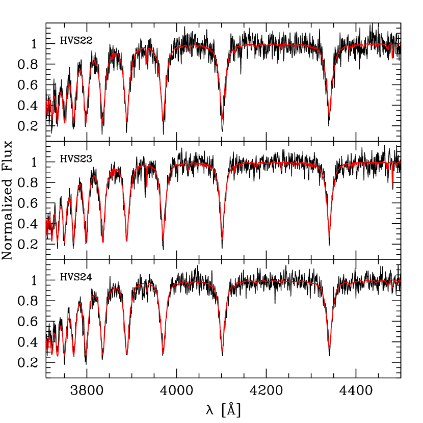
Figure 2.— HVS discovery spectra, continuum-normalized and shifted to rest-frame (in black), compared with the best-fitting stellar atmosphere models (red).

2.4. New HVSs

We find three HVSs in our new observations. The star SDSS J114146.45+044217.29, hereafter HVS22, is a faint $g=20.261\pm 0.042$ and fast-moving $v_{helio}=597.8\pm 13.4$ km s^-1 object. Its minimum velocity in the Galactic rest frame is +489 km s^-1. We compare its broadband colors with stellar evolution tracks and estimate that HVS22 is 70 kpc distant if a BHB star, and 100 kpc distant if a main sequence star. HVS22 is clearly unbound to the Milky Way at either distance. Curiously, HVS22 is located in the constellation Virgo near many of the other HVSs. Figure 2 shows its spectrum.

The star SDSS J215629.02+005444.18, hereafter HVS23, is another faint $g=20.401\pm 0.027$ star but located in the southern Galactic cap. Its broadband colors imply HVS23 is 70 kpc distant if a BHB star, and 80 kpc distant if a main sequence star; HVS23 is unbound at either distance. It’s heliocentric velocity $v_{helio}=259.3\pm 9.9$ km s^-1 is +423 km s^-1 in the Galactic rest frame.

On the basis of follow-up observations, we re-classify SDSS J111136.44+005856.44 as HVS24. HVS24 has a self-consistent set of photometric and spectroscopic distance estimates. Its rest frame velocity $v_{rf}=+361$ km s^-1 is a significant outlier from the observed velocity distribution, and exceeds the Galactic escape velocity at HVS24’s likely distance of $R=63\pm 11$ kpc. Its rapid rotation, described in the next Section, makes HVS24 a probable main sequence B star. HVS24 is also located in the constellation Leo near many of the other HVSs.

3. HVS STELLAR NATURE

Determining the stellar nature of HVSs is important for making accurate distance estimates and for placing constraints on HVS ejection models. We investigate the nature of HVSs by performing stellar atmosphere fits to the entire sample of HVSs. The HVSs, unlike the other stars in the HVS Survey, were observed multiple times to validate their radial velocities, and the summed HVS spectra have signal-to-noise of 40–70 per resolution element adequate for fitting stellar atmosphere models. Heber et al. (2008b) performed similar stellar atmosphere fits to the earliest HVS discoveries, and we now extend this analysis to the full sample of HVSs.

A notable result of the stellar atmosphere fits is that six of our HVSs are fast rotators with $v\sin{i}$$>170$ km s^-1. Fast rotation is the unambiguous signature of a main sequence star. Late B-type main sequence stars have mean $v\sin{i}$$=150$ km s^-1 (Abt et al., 2002; Huang & Gies, 2006); evolved BHB stars have mean $v\sin{i}$$=10$ km s^-1 (Behr, 2003). On this basis, we compare the HVS atmosphere parameters to main sequence tracks to estimate masses and luminosities.

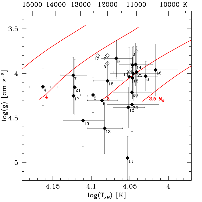
Figure 3.— Derived effective temperature $T_{\rm eff}$ and surface gravity $\log{g}$ compared with Padova solar metallicity main sequence tracks for 2.5, 3, 4, and 5 $M_{\odot}$ stars (red lines). Parameters derived from echelle spectra for the 4 brightest HVSs (open diamonds) are shown for comparison.

3.1. Stellar Atmosphere Fits

Our approach to stellar atmosphere fits is identical to that described by Brown et al. (2012a). In brief, we use ATLAS9 ODFNEW model atmosphere grids (Castelli & Kurucz, 2004; Castelli et al., 1997) to calculate synthetic spectra (Gray & Corbally, 1994) matched to the spectral resolution of our observations. We sum the rest-frame spectra of each HVS, normalize the continuum with a low-order polynomial fit, and calculate the $\chi^{2}$ of the temperature- and gravity-sensitive Balmer lines against the synthetic models. Finally, we fit the resulting distribution of $\chi^{2}$ to derive the best-fitting parameters and uncertainties. We find that $T_{\rm eff}$ and $\log{g}$ are correlated. A 1% increase in $T_{\rm eff}$ best fits a 1% increase in $\log{g}$. Our average uncertainties are $\pm$5%, or $\pm$600 K, in $T_{\rm eff}$ and $\pm$6%, or $\pm$0.24 dex, in $\log{g}$.

Figure 2 shows the spectra for the new objects HVS22, HVS23, and HVS24 compared to their best-fit stellar atmosphere model (note that we calculate $\chi^{2}$ using the spectral regions around each Balmer line, and exclude the continuum regions used for normalization). We summarize $T_{\rm eff}$ and $\log{g}$ values in Table 1 and plot them in Figure 3.

We validate our stellar atmosphere fits by comparing with previously published results. Heber et al. (2008b) perform independent stellar atmosphere fits to our spectra of HVS1 and HVS4-7. For this set of 5 objects, our values are on average $400\pm 400$ K hotter and $0.20\pm 0.11$ dex higher in surface gravity, consistent within the 1-$\sigma$ uncertainties but suggesting a possible systematic offset. Stellar atmosphere fits to high resolution echelle spectra have also been published for the four brightest HVSs: HVS5 (Brown et al., 2012a), HVS7 (López-Morales & Bonanos, 2008; Przybilla et al., 2008b), HVS8 (López-Morales & Bonanos, 2008), and HVS17 (Brown et al., 2013a). For this small set of 4 objects, our values are on average $600\pm 400$ K hotter and $0.30\pm 0.10$ dex higher in surface gravity, again suggesting a systematic offset at the level of our 1-$\sigma$ measurement uncertainty. The systematic offset makes little difference to our stellar mass estimates because the direction of the $T_{\rm eff}$–$\log{g}$ correlation parallels the stellar evolution tracks, but higher surface gravity causes us to systematically under-estimate luminosity and thus distance. The possible systematic therefore acts as a conservative threshold on our identification of unbound HVSs. Given the higher precision of the echelle observations, we adopt echelle $T_{\rm eff}$ and $\log{g}$ values when available.

Figure 4.— Cumulative distribution of HVS projected rotation $v\sin{i}$. Six HVSs have significant rotation $v\sin{i}$$>$170 km s^-1, the unambiguous signature of main sequence B stars.

3.2. Stellar Rotation

Our 1 Å spectral resolution formally allows measurement of the projected stellar rotation for stars with $v\sin{i}$$>$70 km s^-1. The unresolved line Mg ii $\lambda$4481, the strongest unblended metal line in the HVS spectra, in principle provides the best $v\sin{i}$ constraint. In practice, our moderate spectral resolution and moderate S/N, combined with the nearby He i $\lambda$4471 line, makes the Mg ii $\lambda$4481 $v\sin{i}$ measurement difficult. Instead, we rely on the shape of the well-sampled Balmer line profiles. We find a clear minimum in $\chi^{2}$ when fitting model grids over $v\sin{i}$, but the shallow change in $\chi^{2}$ implies large uncertainties. We compare our $v\sin{i}$ with the four HVSs with echelle measurements and the independent measurement of HVS1, and find that our $v\sin{i}$ values are consistent within $\pm 33$ km s^-1. Thus, while we do not claim precise $v\sin{i}$ measurements, we can claim that HVSs with $v\sin{i}$$>$170 km s^-1 have $>$70 km s^-1 rotation at 3-$\sigma$ confidence.

Fast rotation is interesting because it is the clear signature of a main sequence B star. Evolved BHB stars and main sequence B stars have very different $v\sin{i}$, as explained above. Interestingly, the mean $v\sin{i}$ we measure for the HVS sample is 149 km s^-1, equal to the expected mean for a sample of main sequence B stars (Abt et al., 2002; Huang & Gies, 2006). This consistency is suspect, however, as the practical lower limit of our $v\sin{i}$ measurements is about 70 km s^-1. Figure 4 plots the cumulative distribution of $v\sin{i}$.

The six HVSs with 200 to 300 km s^-1 rotation in Figure 4 are remarkable. HVS8 is a previously known fast rotator with $v\sin{i}$=260 km s^-1 (López-Morales & Bonanos, 2008), but HVS9, HVS13, HVS16, HVS20, and HVS24 are new discoveries. In addition, HVS1, HVS6, and HVS14 have $v\sin{i}$’s very near 170 km s^-1 (see also Heber et al., 2008b). Including the HVSs with echelle $v\sin{i}$ measurements, 12 (57%) of our 21 HVSs are probable main sequence B stars on the basis of their rotation.

3.3. Mass and Luminosity Estimates

Given the observed rotation of the HVSs, we adopt main sequence stellar evolution tracks to estimate their masses and luminosities. Previously, we used photometric colors and Padova tracks (Girardi et al., 2004; Marigo et al., 2008) to estimate HVS luminosities. We now use our spectroscopic $T_{\rm eff}$ and $\log{g}$ with the same tracks for consistency. We note that the latest version of the Padova tracks adopt a different value for solar metallicity (Bressan et al., 2012), but metallicity is one of the least constrained of the HVSs’ stellar parameters. Among the objects with echelle spectroscopy, HVS5 and HVS8 provide no metallicity constraint because of their fast rotation. HVS7 and HVS17 have peculiar abundance patterns and so provide no metallicity constraint because of diffusion processes in the radiative atmospheres of the stars. Because these four HVSs are main sequence B stars, however, they must have formed relatively recently in the Milky Way, presumably with approximately solar metallicity. Furthermore, the two HVSs with measurable iron lines both have solar iron abundance. We therefore adopt solar metallicity stellar evolution tracks for estimating HVS parameters.

Figure 3 compares measured $T_{\rm eff}$ and $\log{g}$ to solar metallicity Padova tracks. The HVSs overlap the tracks for 2.5 - 4 $M_{\odot}$ main sequence stars, consistent with the underlying color selection. HVS11 is the only significant outlier. Its $\log{g}$$\simeq$5 is suspiciously close to the edge of the Kurucz model grid, but, if correct, may indicate that HVS11 is an extremely low mass white dwarf like others found in the HVS Survey (Kilic et al., 2007a; Brown et al., 2013b). HVS11 shows no short- or long-term velocity variability, however, arguing against the low mass white dwarf interpretation.

We estimate stellar mass and luminosity using a Monte Carlo calculation to propagate the spectroscopic $T_{\rm eff}$ and $\log{g}$ uncertainties through the tracks. Thus the parameters for objects like HVS11, HVS12, and HVS19, which sit below the main sequence tracks, are determined by the portion of their error ellipse that falls on the tracks. Table 1 summarizes the stellar mass and luminosity estimates.

Our spectroscopic luminosity estimates are formally no more precise than our old photometric estimates, but they are arguably more accurate. The mean uncertainty of our spectroscopic absolute magnitude is $\pm$0.32 mag; the uncertainty of the photometric absolute magnitude is $\pm$0.25 mag. The difference between the spectroscopic and photometric absolute magnitude $M_{g}$ estimates is $0.0\pm 0.39$ mag; the dispersion is consistent with the sum of the uncertainties. HVS1 happens to be one of the most discrepant objects: HVS1’s relatively red $(u-g)$ color corresponds to a star with $M_{g,phot}=+0.42$, yet its hydrogen Balmer lines correspond to a star with $M_{g,spec}=-0.35$. We adopt the spectroscopic estimate throughout. Spectroscopic line profiles are immune to issues such as photometric conditions and filter zero-point calibrations. Thus we consider spectroscopic measures of $T_{\rm eff}$ and $\log{g}$ provide the more accurate estimates of $M_{g}$.

4. HVS SPATIAL AND FLIGHT TIME DISTRIBUTIONS

The spatial and flight time distributions of HVSs can place useful constraints on their origin. We begin by adopting an escape velocity profile for the Milky Way to define our sample of 21 unbound HVSs. The unbound 2.5 - 4 $M_{\odot}$ HVSs we observe imply there are $\simeq$100 such HVSs over the entire sky within $R<100$ kpc. The ratio of HVS flight time to main sequence lifetime implies that the HVSs are ejected at random times during their lives. Thus the apparent number of HVSs must be corrected for their finite lifetimes.

The unbound HVSs exhibit a remarkable spatial anisotropy on the sky: half of the HVSs lie within a region only 15$\arcdeg$ in radius. However, this apparent grouping of HVSs is equally likely to share a common flight time as to be ejected continuously.

4.1. HVS Spatial Distribution

We calculate HVS Galacto-centric radial distances, $R$, assuming the Sun is at $R=8$ kpc. Table 1 summarizes the results. Figure 5 displays the Galacto-centric radial distances as a function of minimum Galactic rest frame velocity $v_{rf}$. Our average 32% absolute magnitude uncertainty corresponds to a 16% distance uncertainty.

Figure 6 visualizes the spatial distribution of HVSs in Galactic cylindrical coordinates. The y-axis in Figure 6 is the vertical distance above the disk, the x-axis is the radial distance along the disk, and the length of the arrows indicates the relative motion of the HVSs. The HVSs are presently located at the arrow tips, and span a large range of distances. Arrows drawn in magenta are the HVSs located in the clump around the constellation Leo. To properly establish our sample of unbound HVSs we must define the escape velocity of the Milky Way.

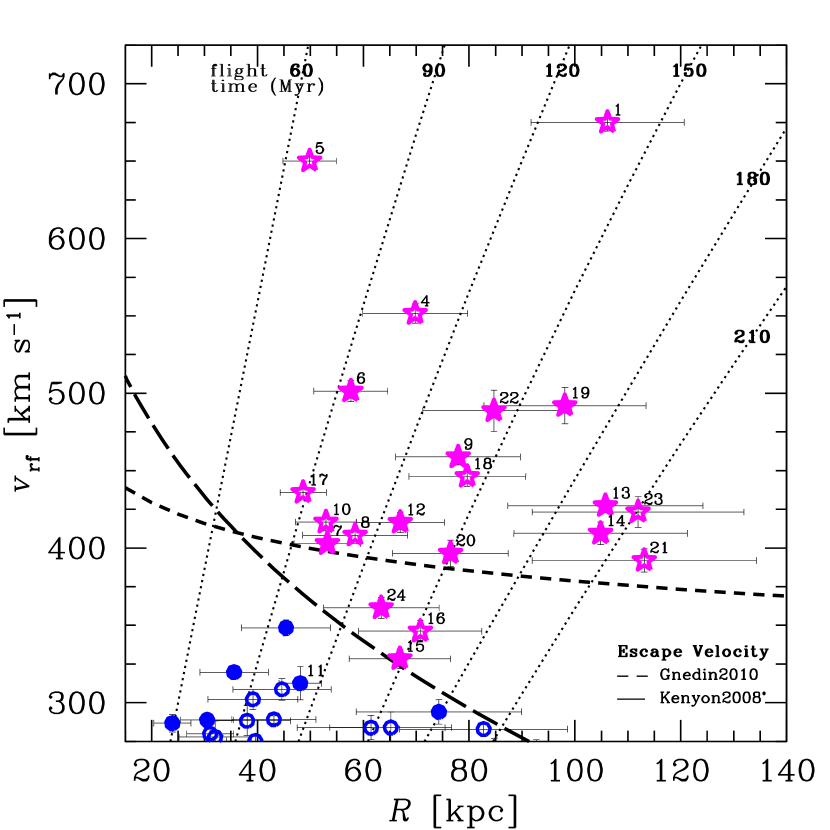
Figure 5.— Galactic rest frame velocity $v_{rf}$ versus Galactocentric distance $R$. We adopt the escape velocity derived from the updated Kenyon et al. (2008) three component bulge-disk-halo model; we show the scaled circular velocity profile measured by Gnedin et al. (2010) for comparison. Unbound HVSs are marked by magenta stars; possible bound HVSs are marked by blue circles. Filled symbols are those objects clumped together around Leo. Dotted lines are isochrones of flight time from the Galactic center.

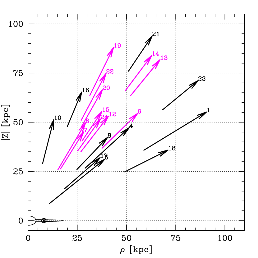
Figure 6.— HVSs plotted in Galactic cylindrical coordinates. Arrow lengths are scaled to $v_{rf}$, and arrow tips are located at the present positions of the HVSs. Magenta arrows are those objects clumped together around Leo.

4.2. Galactic Escape Velocity

The escape velocity of the Milky Way varies with distance because of the Galaxy’s extended mass distribution. We estimate the Milky Way’s escape velocity using an updated version of the Kenyon et al. (2008) three component bulge-disk-halo potential model that fits observed mass measurements. We adopt a new disk mass $M_{d}=6\times 10^{10}$ $M_{\odot}$ and radial scale length $a_{d}=2.75$ kpc that yields a flat 235 km s^-1 rotation curve, consistent with our adopted circular velocity. We leave the other potential model parameters unchanged. Compared to the original Kenyon et al. (2008) model, our updated model contains more disk mass and thus requires a slightly larger ejection velocity to escape.

Escape velocity is not formally defined in the three-component potential model. We empirically estimate escape velocity by dropping a test particle from the virial radius at 250 kpc. The resulting escape velocity curve drawn in Figure 5 can be fit with the following relation, valid in the range $15<R<150$ kpc:

$$v_{esc}(R) =624.9-9.4136R+0.134197R^{2}-1.28165\times 10^{-3}R^{3}$$ (2)

$$+6.47686\times 10^{-6}R^{4}-1.31814\times 10^{-8}R^{5}.$$

Our adopted potential model yields an escape velocity of 366 km s^-1 at $R=50$ kpc and 570 km s^-1 at $R=8$ kpc. The latter value is consistent with current solar neighborhood escape velocity measurements (Smith et al., 2007; Piffl et al., 2013).

An alternative escape velocity estimate is provided by scaling the halo circular velocity measured by Gnedin et al. (2010) from a Jeans analysis of the Milky Wau stellar halo velocity dispersion profile. The inferred escape velocity in this case is 400 km s^-1 at $R=50$ kpc (see Figure 5). Scaling circular velocity to estimate escape velocity is formally incorrect, however. More recently, Rashkov et al. (2013) argue that the Milky Way halo is significantly less massive than assumed by Kenyon et al. (2008) and measured by Gnedin et al. (2010). Given the uncertainties, we consider the updated Kenyon et al. (2008) escape velocity model a reasonable choice.

Given the above definition of escape velocity, we identify 21 HVSs that are unbound on the basis of radial velocity alone (Figure 5). We include HVS16 and HVS24 because they sit well above the Kenyon et al. (2008) escape velocity curve and have $v\sin{i}$$>$200 km s^-1. Thus HVS16 and HVS24 are $\simeq$3 $M_{\odot}$ B stars at 60–70 kpc distances. HVS15 is a borderline case that we consider a likely HVS because of its significant $v_{rf}=328$ km s^-1 velocity and its self-consistent photometric and spectroscopic distance estimates.

HVS11, given our new distance estimate, is an object that we now classify as a possible “bound HVS.” In fact, we consider all of the remaining objects with 275 km s^-1 $<v_{rf}<v_{esc}$ as possible bound HVSs: significant velocity outliers that are bound. Our choice of 275 km s^-1 is motivated by the relative absence of stars with velocities less than $-275$ km s^-1 in our Survey. We emphasize that our choice of the 275 km s^-1 threshold is appropriate only in the context of our halo radial velocity survey, and is not a generalizable threshold on which to select HVSs in other contexts, such as the solar neighborhood or the Galactic center (e.g. Zubovas et al., 2013) where escape velocity is very different.

Figure 7.— Ratios of HVS flight time to main sequence lifetime. An average ratio of 0.5 suggests that HVSs are ejected at random times during their main sequence lifetimes.

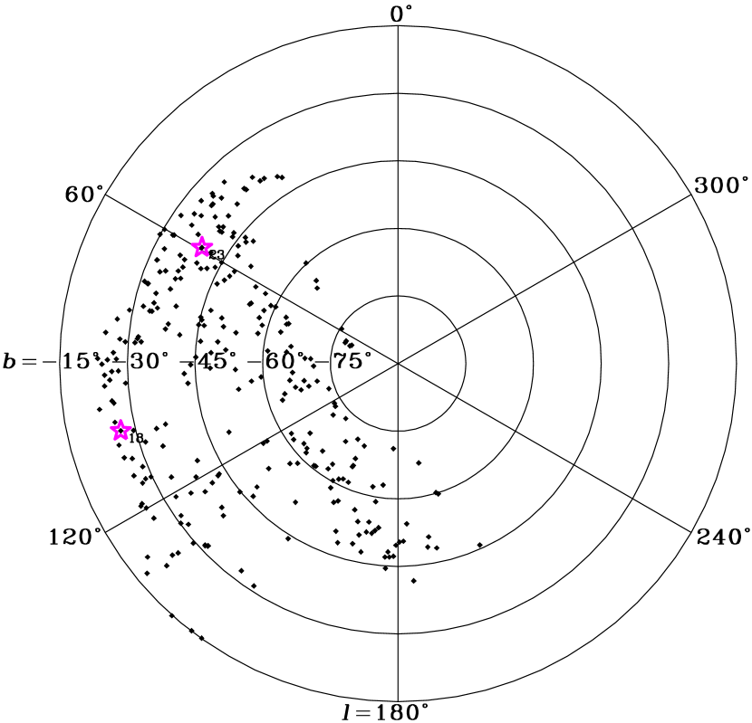
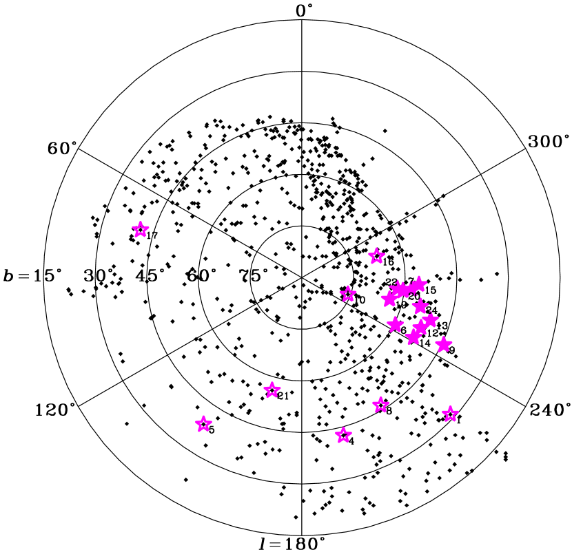
Figure 8.— Polar projections, in Galactic coordinates, showing the spatial distribution of the 1126 late B-type stars in the HVS Survey. Southern Galactic cap is left and the northern Galactic cap is right. The 21 unbound HVSs are marked by magenta stars; filled stars mark the HVSs clumped together around Leo.

4.3. HVS Flight Times and Main Sequence Lifetimes

We now use our distance and velocity measurements to estimate HVS flight times. Our approach is to start at the present location and velocity of each HVS, and then calculate its trajectory backwards through the Galactic center in the updated Kenyon et al. (2008) potential model (see the flight time isochrones in Figure 5). Our flight times are formally upper limits because we assume that the observed radial velocities are the full space motion of the HVSs. This assumption is reasonable for objects on radial trajectories at large 50 - 120 kpc distances. We note that flight times from other locations in the Milky Way, such as the solar circle $R=8$ kpc, typically vary by only $\pm$3 Myr ($\sim$2%) from the Galactic center flight time because of the large distances and high Galactic latitudes of the HVSs. We estimate flight time uncertainties by propagating the velocity and distance errors through our trajectory calculations. Distance errors dominate the uncertainty; thus our typical flight time uncertainties are 16%, or about $\pm$22 Myr.

The difference between flight time and age can constrain a HVS’s origin (Brown et al., 2012a), however our spectroscopic measurements provide no constraint on HVS age. The best we can do is to use our stellar mass estimates to estimate a star’s total main sequence lifetime. In the Padova tracks, the main sequence lifetime of a 3 $M_{\odot}$ star is 350 Myr and a 4 $M_{\odot}$ star is 180 Myr.

Figure 7 compares HVS flight times and main sequence lifetimes. In all cases, the ratios of HVS flight time to main sequence lifetime are less than one. In other words, the HVSs are all consistent with being main sequence stars ejected from the Milky Way. Interestingly, the average ratio of HVS flight time to main sequence lifetime is 0.46. A ratio of one-half suggests that HVSs are ejected at random times during their lives.

4.4. HVS Spatial Anisotropy

The spatial distribution of HVSs is interesting because it is linked to their origin. HVSs can in principle appear anywhere in our 12,000 deg² survey because the central MBH can in principle eject a HVS in any direction. Yet eleven (52%) of the 21 unbound HVSs are located in a $25\arcdeg\times 25\arcdeg$ (5% of Survey area) region at the edge of our survey, centered around (RA, Dec) = ($11^{h}10^{m}00^{s},+3^{d}00^{m}00^{s}$) J2000 in the direction of the constellation Leo.

Figure 8 plots the spatial distribution of every star observed in the HVS Survey in two polar projections centered on the north and south Galactic poles. The overall distribution of stars reflects the SDSS imaging footprint. In this footprint, our Survey stars have an approximately isotropic distribution, although part of the Sgr dwarf galaxy tidal stream is visible as an overdensity of stars arcing to the right of the north Galactic pole (King et al., 2012). The unbound HVSs are marked by magenta stars in Figure 8. The new HVS discoveries strengthen the previously claimed HVS spatial anisotropy. By any measure, whether Galactic longitude distribution, angular separation distribution, or the two-point angular correlation function, unbound HVSs are significantly clustered (see Brown et al., 2009b, 2012b). The lower velocity, possible bound HVSs have a more isotropic distribution.

Various models have been proposed to explain the HVS anisotropy. Each model predicts different spatial and flight time distribution of HVSs. One model is the in-spiral of two massive black holes in the Galactic center (Gualandris et al., 2005; Levin, 2006; Sesana et al., 2006; Baumgardt et al., 2006). A binary black hole preferentially ejects HVSs from its orbital plane; thus HVSs ejected by a binary black hole in-spiral event should form a ring around the sky. Models predict a binary black hole will harden and merge on $\sim$1 Myr timescales (Sesana et al., 2008). Thus the signature of a single in-spiral event is a ring of HVSs with a common flight time.

Abadi et al. (2009) propose that the HVS anisotropy comes from the stellar ejecta of a tidally disrupted dwarf galaxy (see also Piffl et al., 2011). This model predicts a single clump of HVS with a common flight time. However, it is unclear where the progenitor would come from. No Local Group dwarf galaxy has a velocity comparable to the HVSs, and a gas-rich star forming galaxy is required to explain the B-type HVSs. There are no unbound A- or F-type stars in same region of sky (Kollmeier et al., 2009, 2010) as one expects for a disrupted dwarf galaxy.

Lu et al. (2010) and Zhang et al. (2010, 2013) propose that the HVS anisotropy reflects the anisotropic distribution of stars in the Galactic center. If HVSs are ejected by the central MBH, then the direction of ejection corresponds to the direction that their progenitors encounter the MBH. Interestingly, known HVSs fall on the projected orbital planes of the clockwise and counter-clockwise disks of stars that presently orbit Sgr A*. There is no explanation for the confinement of HVS ejections to two fixed planes over the past 200 Myr, however. If we accept fixed ejection planes, this model allows for bands of HVSs on the sky containing stars of all possible flight times.

Finally, Brown et al. (2012b) propose that the HVS anisotropy may reflect the anisotropy of the underlying Galactic gravitational potential. Stars ejected along the long axis of the potential are decelerated less than those ejected along the minor axis. An initially isotropic distribution of marginally unbound HVSs can thus appear anisotropic in the halo. The predicted distribution of HVSs depends on the axis ratio and the rotation direction of the potential. If there is rotation around the long axis of the potential, for example, HVSs should appear in two clumps on opposite sides of the sky with all possible flight times.

Although the present spatial distribution of HVSs can be described by two planes (Lu et al., 2010; Zhang et al., 2010), this is not necessarily the required distribution. The observed clump of HVSs abuts one edge of the Survey – the edge defined by the celestial equator. We require a southern hemisphere HVS Survey to see the full all-sky distribution. For now, we simply test whether the observed clump of HVSs share a common flight time.

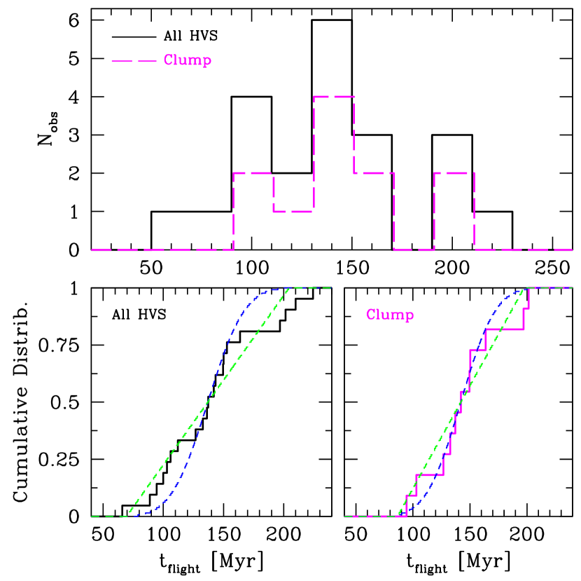
Figure 9.— Distribution of HVS flight times from the Galactic center, in 20 Myr bins (upper panel). The subset of HVSs clumped together around Leo are drawn in magenta. Lower panels plot the cumulative distributions of the full sample (left) and the clumped sample (right) compared to a continuous distribution and a Gaussian distribution with a 24 Myr dispersion.

4.5. Flight Time Constraints on Origin

HVS flight times provide another constraint on origin. Figure 9 plots the distribution of flight times for the full sample of HVSs and for the clump of HVSs within 15$\arcdeg$ of $11^{h}10^{m}00^{s},+3^{d}00^{m}00^{s}$ (J2000). We make this particular selection because it cuts the HVS sample in half, and allows us to test the dwarf galaxy tidal debris hypothesis. We calculate the non-parametric Kolmogorov-Smirnov statistic of the samples against two models. The first model is a constant distribution, normalized to the number of HVSs and centered on the mean $t_{flight}$ of each HVS sample. The second model is a burst distribution: a Gaussian with identical mean and normalization as the first model, but a dispersion equal to 16% of the mean $t_{flight}$ appropriate for our measurement uncertainties. The lower panels of Figure 9 compare these models to the observed cumulative distribution of HVS flight times.

The full HVS sample is well-described by a continuous flight time distribution (KS probability 0.80) but poorly described by a single burst (KS probability 0.08). The spatially clumped HVS flight times, on the other hand, are equally well-described by a continuous distribution (KS probability 0.89) and a single burst (KS probability 0.83). Thus we can neither confirm nor deny the tidal debris origin on the basis of the spatially clumped HVS flight times. On the other hand, the flight times of the full set of HVSs rule out a single burst. In other words, if HVSs are ejected by binary MBH in-spiral or dwarf galaxy tidal disruption events, the data require multiple events to explain the full HVS sample.

5. HVS PROPER MOTION PREDICTIONS

Proper motions may one day provide a direct constraint on HVS origin. The proper motions of the HVSs remain unmeasured except in special cases (Brown et al., 2010a), because the HVSs are distant and their proper motions are too small $\lesssim$1 mas yr^-1 to be measured in ground-based catalogs. Gaia promises to measure proper motions for the HVSs with 0.1 mas yr^-1 precision. These measurements will, in many cases, discriminate between Galactic center and disk origins.

Here, we lay the groundwork for interpreting future proper motion measurements by 1) predicting the proper motion HVSs must have if they come from the Galactic center, and 2) calculating the ejection velocities required for alternative Galactic disk origins. Similar calculations were done for early HVS discoveries (Svensson et al., 2008). Here we address the full sample of unbound HVSs.

Our computational approach is to step through a grid of all possible proper motions and calculate the corresponding HVS trajectories backwards in time through the updated Kenyon et al. (2008) potential model. For each trajectory we record Galactic plane-crossing location and velocity, and we calculate the necessary Galactic disk ejection velocity assuming a flat 235 km s^-1 rotation curve.

Figure 10 shows how the trajectories for each HVS map onto proper motion space: the blue and green ellipses are the locus of proper motions with trajectories crossing the Galactic plane at $R=20$ kpc and $R=8$ kpc, respectively. We identify a Galactic center origin by the trajectory with the smallest Galactic pericenter passage. An x marks this trajectory, and Table 1 lists the corresponding proper motion for the Galactic center origin.

Our trajectory calculations place interesting constraints on a disk origin. Theorists show that the maximum possible ejection velocity from stellar binary-binary interactions is, under a point mass assumption, the escape velocity from the surface of the most massive star (Leonard, 1991). The escape velocity from the surface of a 3 $M_{\odot}$ main sequence star is $\simeq$600 km s^-1. Thus, the only locations where HVSs can be ejected by stellar runaway mechanisms are those locations in the disk where the ejection velocity is below 600 km s^-1. The red contours in Figure 10 shows this constraint for each HVS. Trajectories with disk ejection velocities $<$600 km s^-1 have proper motions that lie inside the red contour.

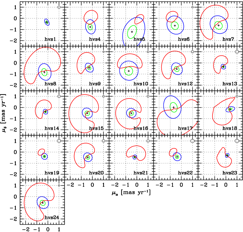
Figure 10.— HVS trajectories mapped into proper motion space. Green and blue ellipses are the locus of trajectories that pass within 8 and 20 kpc, respectively, of the Galactic center. Trajectories that pass through the Galactic center are marked by an +. The locus of trajectories with disk plane ejection velocities of 600 km s^-1, the escape velocity from the surface of a 3 $M_{\odot}$star, are indicated by the red contours. Physically allowed disk ejections are mostly limited to the outer disk. Black circles are the predicted Gaia proper motion error ellipses for each HVS.

Interestingly, there is no location where HVS1 can physically be ejected from the Galactic disk. Due to its extreme velocity and distance, HVS1 provides a strong case for a Galactic center origin. For the other HVSs, there are finite but limited portions of the disk from where they can be ejected. The lowest disk ejection velocities occur where disk rotation points towards the HVSs. Minimum disk ejection velocities range 400–590 km s^-1. The average radial location of the minima is $R=28$ kpc, however, well outside the Milky Way’s stellar disk. Only HVS5, with a disk ejection velocity of 590 km s^-1 at $R=18$ kpc, has a minimum that falls within the $R\simeq 20$ kpc extent of the observed stellar disk. The viable region for HVS disk ejections is thus typically a small fraction of the disk; it is the area included within both the blue and red contours in Figure 10.

Notably, a Galactic center origin is often well-separated in proper motion from a disk origin. This separation occurs because viable disk ejection trajectories are from the outer disk. Future proper motion measurements with 0.1 mas yr^-1 precision should thus be able to distinguish between Galactic center and disk origins. Gaia astrometric performance specifications predict 0.035 - 0.17 mas yr^-1 proper motion uncertainties for the HVSs; the error ellipses depend on apparent magnitude and are drawn as the black circles in the upper right-hand corners of the panels in Figure 10. If Gaia meets its predicted astrometric performance, it should unambiguously determine the origin of HVS4, HVS5, HVS6, HVS7, HVS8, HVS9, HVS10, and HVS17.

6. DISCUSSION AND CONCLUSIONS

The HVS Survey is a complete, color-selected sample of late B-type stars over 12,000 deg² (29%) of sky. Spectroscopy of these stars reveals 21 HVSs unbound in radial velocity alone. The Survey also identifies a comparable number of velocity outliers that are possibly bound HVSs. Stellar atmosphere fits show that, on the basis of projected stellar rotation, at least half of the HVSs are certain main sequence 2.5 - 4 $M_{\odot}$ stars at 50 - 120 kpc distances.

If we assume that the HVSs are ejected continuously and isotropically, the 21 observed HVSs implies there are $\simeq$100 unbound 2.5 - 4 $M_{\odot}$ HVSs over the entire sky within $R<100$ kpc. This calculation neglects HVSs missing from our Survey because of their short lifetimes, however. In previous papers, we corrected the observed number of HVSs by the fraction that do not survive to reach large distances assuming the HVSs are ejected at zero age (Bromley et al., 2006; Brown et al., 2007c). This assumption is flawed, as demonstrated by the observed ratios of HVS flight time to main sequence lifetime. If we instead assume that HVSs are ejected at any time during their lifetime, then we expect about 32% of 2.5 - 4 $M_{\odot}$ HVSs do not survive to reach 50 kpc, and 64% do not survive to reach 100 kpc. The corrected number of HVSs is $\simeq$300 unbound 2.5 - 4 $M_{\odot}$ HVSs over the entire sky within $R<100$ kpc. The ejection rate of unbound 2.5 - 4 $M_{\odot}$ HVSs is thus $1.5\times 10^{-6}$ yr^-1.

To infer a total HVS ejection rate requires many more assumptions. The simplest approach is to assume that all stellar masses have identical binary fractions, binary orbital distributions, and ejection velocities, and then scale the observed 2.5 - 4 $M_{\odot}$ HVSs by an assumed mass function. For a Salpeter IMF, integrated over the mass range $0.1<M<100$ $M_{\odot}$ and scaled to the corrected number of 2.5 - 4 $M_{\odot}$ HVSs, the total HVS ejection rate is $2.5\times 10^{-4}$ yr^-1. This rate is comparable to the $10^{-4}$ yr^-1 HVS ejection rates predicted by theory (Hills, 1988; Perets et al., 2007; Zhang et al., 2013). It is difficult to take the ejection rate calculation further because the properties of binary stars and the stellar mass function in the Galactic center are poorly constrained. However, the general agreement between HVS observation and HVS theory is a good consistently check.

The distribution of HVS flight times provides another constraint on origin. HVSs ejected by a single MBH can be observed with any flight time. HVSs ejected by a dwarf galaxy tidal disruption event or a binary MBH in-spiral event must share a common flight time. Our full HVS sample is well-described by a continuous flight time distribution, but poorly described by a single burst. This conclusion is consistent with the Hills (1988) scenario. Alternatively, this conclusion requires multiple binary MBH in-spiral or galaxy tidal disruption events.

An intriguing result remains the anisotropic HVS spatial distribution: half of the observed HVSs are located around the constellation Leo. Because the HVSs are clumped at the edge of our Survey, the true distribution of HVSs remains unknown. The flight times of the spatially clumped HVSs also provide no constraint; the flight times of the clump are equally well-described by a continuous distribution or a single burst.

In the near future, proper motions promise to provide a direct test of HVS origin. The first unbound main sequence star with measured proper motion is HD 271791 (Heber et al., 2008a), a runaway B star ejected in the direction of rotation from the outer disk by a stellar binary disruption process (Przybilla et al., 2008a; Gvaramadze et al., 2009). Stellar binary disruption processes have a speed limit, however, set by the escape velocity from the surface of the star. We perform trajectory calculations for our HVSs and show that, in many cases, physically allowed disk-ejection trajectories differ systematically from Galactic center trajectories in proper motion space. Proper motions with 0.1 mas yr^-1 precision, possible with Hubble Space Telescope and Gaia, should place clear constraints on the origin of HVSs 4 - 10 and HVS17.

We also look forward to performing a southern hemisphere HVS Survey in the near future. Whether the HVSs are ejected in rings, clumps, or a more isotropic distribution is an important constraint on their origin. Doubling the sample of HVSs to $\sim$50 objects should also allow us to discriminate between single and binary MBH ejection mechanisms on the basis of the HVS velocity distribution (Sesana et al., 2007; Perets, 2009). Ejection models predict $>$1,000 km s^-1 stars (e.g. Bromley et al., 2006; Sesana et al., 2007; Zhang et al., 2010; Rossi et al., 2014), stars that are not yet observed. We expect that full sky coverage provided by surveys like SkyMapper (Keller et al., 2007) will provide a rich source of future HVS discoveries.

Table 1HVS Survey Stars with $v_{rf}>+275$ km s^-1

HVS	$v_{\sun}$	$v_{rf}$	$g_{0}$	$T_{\rm eff}$	$\log{g}$	$v\sin{i}$	mass	$M_{g}$	$R_{GC}$	$t_{flight}$	$(\mu_{\alpha},~{}\mu_{\delta})_{GC}$	Catalog
	(km s-1)	(km s-1)	(mag)	(K)	(cm s-2)	(km s-1)	($M_{\odot}$)	(mag)	(kpc)	(Myr)	(mas yr-1)
HVSs
1	$833.0\pm 5.5$	675.0	19.688	$11125\pm 463$	$3.91\pm 0.20$	162	$3.21\pm 0.13$	$-0.34\pm 0.31$	$106\pm 14$	$136\pm 19$	$-0.09,-0.35$	SDSS J090744.99$+$024506.89
4	$600.9\pm 6.2$	551.5	18.314	$14547\pm 607$	$4.15\pm 0.21$	77	$4.24\pm 0.16$	$-0.71\pm 0.34$	$70\pm 10$	$106\pm 17$	$-0.20,-0.77$	SDSS J091301.01$+$305119.83
5	$545.5\pm 4.3$	650.1	17.557	$12000\pm 350$	$3.89\pm 0.13$	132	$3.58\pm 0.11$	$-0.68\pm 0.25$	$50\pm 5$	$66\pm 7$	$-0.44,-1.21$	SDSS J091759.47$+$672238.35
6	$609.4\pm 6.8$	501.4	18.966	$12190\pm 546$	$4.30\pm 0.23$	170	$3.06\pm 0.11$	$+0.25\pm 0.28$	$58\pm 7$	$94\pm 13$	$-0.58,-0.66$	SDSS J110557.45$+$093439.47
7	$527.8\pm 2.7$	402.8	17.637	$12000\pm 500$	$3.80\pm 0.10$	62	$3.76\pm 0.13$	$-0.95\pm 0.27$	$53\pm 6$	$103\pm 12$	$-0.65,-0.63$	SDSS J113312.12$+$010824.87
8	$499.3\pm 2.9$	408.3	17.939	$11000\pm 1000$	$3.75\pm 0.25$	320	$3.42\pm 0.20$	$-0.70\pm 0.40$	$58\pm 10$	$112\pm 19$	$-0.31,-0.84$	SDSS J094214.03$+$200322.07
9	$616.8\pm 5.1$	458.8	18.639	$11680\pm 529$	$3.83\pm 0.21$	294	$3.56\pm 0.16$	$-0.74\pm 0.34$	$78\pm 12$	$137\pm 21$	$-0.29,-0.44$	SDSS J102137.08$-$005234.77
10	$467.9\pm 5.6$	416.7	19.220	$11270\pm 533$	$4.38\pm 0.23$	64	$2.65\pm 0.11$	$+0.65\pm 0.24$	$53\pm 6$	$100\pm 12$	$-0.73,-0.73$	SDSS J120337.85$+$180250.35
12	$552.2\pm 6.6$	416.5	19.609	$12098\pm 632$	$4.62\pm 0.28$	78	$2.73\pm 0.14$	$+0.56\pm 0.28$	$67\pm 8$	$127\pm 17$	$-0.41,-0.55$	SDSS J105009.59$+$031550.67
13	$572.7\pm 4.5$	427.3	20.018	$11241\pm 739$	$4.04\pm 0.33$	189	$3.07\pm 0.17$	$-0.07\pm 0.39$	$106\pm 18$	$197\pm 37$	$-0.23,-0.34$	SDSS J105248.30$-$000133.94
14	$537.3\pm 7.2$	409.4	19.717	$11030\pm 554$	$3.90\pm 0.24$	162	$3.18\pm 0.15$	$-0.33\pm 0.35$	$105\pm 16$	$202\pm 32$	$-0.22,-0.38$	SDSS J104401.75$+$061139.02
15	$461.0\pm 6.3$	328.3	19.153	$11132\pm 535$	$4.05\pm 0.23$	125	$2.99\pm 0.12$	$+0.05\pm 0.32$	$67\pm 10$	$150\pm 23$	$-0.46,-0.52$	SDSS J113341.09$-$012114.25
16	$429.8\pm 7.0$	346.2	19.334	$10388\pm 666$	$3.96\pm 0.29$	259	$2.85\pm 0.15$	$+0.07\pm 0.36$	$71\pm 12$	$153\pm 26$	$-0.50,-0.51$	SDSS J122523.40$+$052233.84
17	$250.2\pm 2.9$	435.8	17.427	$12350\pm 290$	$3.80\pm 0.09$	96	$3.91\pm 0.09$	$-1.05\pm 0.19$	$49\pm 4$	$89\pm 8$	$-0.69,+0.01$	SDSS J164156.39$+$472346.12
18	$237.3\pm 6.4$	446.2	19.302	$11993\pm 516$	$4.08\pm 0.22$	96	$3.27\pm 0.12$	$-0.15\pm 0.31$	$80\pm 11$	$143\pm 22$	$+0.39,-0.16$	SDSS J232904.94$+$330011.47
19	$592.8\pm 11.8$	492.0	20.061	$12900\pm 793$	$4.53\pm 0.29$	137	$3.12\pm 0.17$	$+0.13\pm 0.34$	$98\pm 15$	$164\pm 28$	$-0.31,-0.39$	SDSS J113517.75$+$080201.49
20	$512.1\pm 8.5$	396.6	19.807	$11149\pm 649$	$4.21\pm 0.28$	275	$2.79\pm 0.12$	$+0.42\pm 0.32$	$76\pm 11$	$150\pm 24$	$-0.41,-0.48$	SDSS J113637.13$+$033106.84
21	$356.8\pm 7.5$	391.9	19.730	$13229\pm 998$	$4.16\pm 0.31$	65	$3.70\pm 0.21$	$-0.45\pm 0.42$	$113\pm 21$	$224\pm 48$	$-0.18,-0.45$	SDSS J103418.25$+$481134.57
22	$597.8\pm 13.4$	488.7	20.181	$11145\pm 859$	$4.35\pm 0.30$	94	$2.66\pm 0.15$	$+0.56\pm 0.35$	$85\pm 13$	$142\pm 25$	$-0.38,-0.43$	SDSS J114146.44$+$044217.29
23	$259.3\pm 9.8$	423.2	20.201	$10996\pm 778$	$3.99\pm 0.29$	48	$3.04\pm 0.16$	$-0.10\pm 0.38$	$112\pm 20$	$210\pm 40$	$+0.12,-0.30$	SDSS J215629.01$+$005444.18
24	$496.2\pm 6.8$	361.3	18.855	$11103\pm 806$	$4.00\pm 0.31$	228	$3.06\pm 0.17$	$-0.10\pm 0.39$	$63\pm 11$	$133\pm 25$	$-0.46,-0.56$	SDSS J111136.44$+$005856.44
Possible Bound HVSs
	$148.0\pm 6.9$	308.6	17.139	$12383\pm 1474$	$3.81\pm 0.51$	258	$3.90\pm 0.32$	$-0.94\pm 0.49$	$45\pm 9$	$104\pm 22$	$+0.93,-0.54$	SDSS J002810.33$+$215809.66
	$138.3\pm 6.5$	302.1	17.767	$12403\pm 1632$	$4.54\pm 0.60$	328	$2.99\pm 0.33$	$+0.07\pm 0.54$	$39\pm 9$	$92\pm 22$	$+1.22,-0.55$	SDSS J005956.06$+$313439.29
	$352.7\pm 4.5$	282.8	18.388	$10613\pm 908$	$3.52\pm 0.44$	220	$3.61\pm 0.25$	$-1.00\pm 0.45$	$83\pm 16$	$203\pm 36$	$+0.09,-0.64$	SDSS J074950.24$+$243841.16
	$216.1\pm 4.4$	279.9	17.276	$12027\pm 880$	$4.50\pm 0.37$	176	$2.85\pm 0.19$	$+0.34\pm 0.39$	$31\pm 4$	$77\pm 12$	$-0.19,-2.22$	SDSS J081828.07$+$570922.07
	$298.6\pm 4.3$	275.2	18.081	$11673\pm 798$	$4.46\pm 0.33$	45	$2.74\pm 0.16$	$+0.47\pm 0.35$	$40\pm 5$	$99\pm 15$	$-0.33,-1.54$	SDSS J090710.07$+$365957.54
11	$472.7\pm 10.8$	312.6	19.582	$11296\pm 571$	$4.95\pm 0.24$	142	$2.14\pm 0.11$	$+1.35\pm 0.20$	$48\pm 4$	$111\pm 10$	$-0.43,-0.76$	SDSS J095906.47$+$000853.41
	$218.3\pm 10.2$	283.9	19.829	$10583\pm 1118$	$4.53\pm 0.43$	200	$2.31\pm 0.24$	$+0.93\pm 0.41$	$65\pm 12$	$160\pm 31$	$-0.31,-0.81$	SDSS J101359.79$+$563111.65
	$504.0\pm 5.1$	348.4	18.479	$11230\pm 1066$	$4.24\pm 0.44$	167	$2.82\pm 0.20$	$+0.33\pm 0.43$	$45\pm 8$	$97\pm 21$	$-0.62,-0.75$	SDSS J103357.26$-$011507.35
	$447.7\pm 7.9$	294.1	19.235	$10570\pm 1443$	$3.95\pm 0.56$	302	$2.95\pm 0.26$	$-0.06\pm 0.47$	$74\pm 16$	$178\pm 40$	$-0.31,-0.48$	SDSS J104318.29$-$013502.51
	$482.0\pm 4.0$	319.6	17.381	$11497\pm 863$	$3.97\pm 0.33$	296	$3.26\pm 0.19$	$-0.32\pm 0.41$	$36\pm 6$	$81\pm 16$	$-1.02,-0.76$	SDSS J112255.77$-$094734.92
	$414.8\pm 4.6$	288.9	18.133	$11087\pm 914$	$4.55\pm 0.42$	144	$2.47\pm 0.19$	$+0.76\pm 0.38$	$30\pm 5$	$74\pm 13$	$-1.34,-1.01$	SDSS J115245.91$-$021116.21
	$212.8\pm 2.4$	289.1	17.492	$11767\pm 744$	$3.85\pm 0.29$	43	$3.56\pm 0.19$	$-0.69\pm 0.40$	$43\pm 8$	$104\pm 19$	$-0.98,-0.64$	SDSS J140432.38$+$352258.41
	$280.8\pm 5.7$	286.8	18.399	$11170\pm 830$	$4.92\pm 0.32$	50	$2.14\pm 0.16$	$+1.29\pm 0.30$	$24\pm 4$	$58\pm 9$	$-1.82,-1.03$	SDSS J141723.34$+$101245.74
	$215.1\pm 7.9$	283.9	18.884	$11563\pm 1224$	$4.04\pm 0.48$	152	$3.21\pm 0.24$	$-0.23\pm 0.46$	$61\pm 14$	$151\pm 37$	$-0.56,-0.48$	SDSS J154806.92$+$093423.93
	$71.1\pm 9.7$	288.3	17.510	$11150\pm 1224$	$3.87\pm 0.52$	325	$3.28\pm 0.26$	$-0.44\pm 0.47$	$38\pm 8$	$92\pm 20$	$-0.57,+0.16$	SDSS J180050.86$+$482424.63
	$130.0\pm 10.4$	277.8	17.354	$11993\pm 1303$	$4.16\pm 0.54$	42	$3.21\pm 0.26$	$-0.13\pm 0.48$	$32\pm 7$	$80\pm 19$	$+1.09,-0.88$	SDSS J232229.47$+$043651.45

References

- Abadi et al. (2009) Abadi, M. G., Navarro, J. F., & Steinmetz, M. 2009, ApJ, 691, L63
- Abt et al. (2002) Abt, H. A., Levato, H., & Grosso, M. 2002, ApJ, 573, 359
- Aihara et al. (2011) Aihara, H., Allende Prieto, C., An, D., et al. 2011, ApJS, 193, 29
- Allende Prieto et al. (2008) Allende Prieto, C., Sivarani, T., Beers, T. C., et al. 2008, AJ, 136, 2070
- Baumgardt et al. (2006) Baumgardt, H., Gualandris, A., & Portegies Zwart, S. 2006, MNRAS, 372, 174
- Behr (2003) Behr, B. B. 2003, ApJS, 149, 67
- Bovy et al. (2012) Bovy, J., Allende Prieto, C., Beers, T. C., et al. 2012, ApJ, 759, 131
- Bressan et al. (2012) Bressan, A., Marigo, P., Girardi, L., et al. 2012, MNRAS, 427, 127
- Bromley et al. (2009) Bromley, B. C., Brown, W. R., Geller, M. J., & Kenyon, S. J. 2009, ApJ, 706, 925
- Bromley et al. (2006) Bromley, B. C., Kenyon, S. J., Geller, M. J., Barcikowski, E., Brown, W. R., & Kurtz, M. J. 2006, ApJ, 653, 1194
- Brown et al. (2010a) Brown, W. R., Anderson, J., Gnedin, O. Y., Bond, H. E., Geller, M. J., Kenyon, S. J., & Livio, M. 2010a, ApJ, 719, L23
- Brown et al. (2012a) Brown, W. R., Cohen, J. G., Geller, M. J., & Kenyon, S. J. 2012a, ApJ, 754, L2
- Brown et al. (2013a) —. 2013a, ApJ, 775, 32
- Brown et al. (2009a) Brown, W. R., Geller, M. J., & Kenyon, S. J. 2009a, ApJ, 690, 1639
- Brown et al. (2012b) —. 2012b, ApJ, 751, 55
- Brown et al. (2009b) Brown, W. R., Geller, M. J., Kenyon, S. J., & Bromley, B. C. 2009b, ApJ, 690, L69
- Brown et al. (2010b) Brown, W. R., Geller, M. J., Kenyon, S. J., & Diaferio, A. 2010b, AJ, 139, 59
- Brown et al. (2005) Brown, W. R., Geller, M. J., Kenyon, S. J., & Kurtz, M. J. 2005, ApJ, 622, L33
- Brown et al. (2006a) —. 2006a, ApJ, 640, L35
- Brown et al. (2006b) —. 2006b, ApJ, 647, 303
- Brown et al. (2007a) —. 2007a, ApJ, 666, 231
- Brown et al. (2007b) Brown, W. R., Geller, M. J., Kenyon, S. J., Kurtz, M. J., & Bromley, B. C. 2007b, ApJ, 660, 311
- Brown et al. (2007c) —. 2007c, ApJ, 671, 1708
- Brown et al. (2013b) Brown, W. R., Kilic, M., Allende Prieto, C., Gianninas, A., & Kenyon, S. J. 2013b, ApJ, 769, 66
- Brown et al. (2010c) Brown, W. R., Kilic, M., Allende Prieto, C., & Kenyon, S. J. 2010c, ApJ, 723, 1072
- Brown et al. (2012c) —. 2012c, ApJ, 744, 142
- Castelli et al. (1997) Castelli, F., Gratton, R. G., & Kurucz, R. L. 1997, A&A, 318, 841
- Castelli & Kurucz (2004) Castelli, F. & Kurucz, R. L. 2004, arXiv:astro-ph/0405087
- Do et al. (2013) Do, T., Martinez, G. D., Yelda, S., et al. 2013, ApJ, L6
- Edelmann et al. (2005) Edelmann, H., Napiwotzki, R., Heber, U., Christlieb, N., & Reimers, D. 2005, ApJ, 634, L181
- Fekel (1999) Fekel, F. C. 1999, in ASP Conf. Ser. 185: IAU Colloq. 170: Precise Stellar Radial Velocities, ed. J. B. Hearnshaw & C. D. Scarfe (San Francisco: ASP), 378
- Fuentes et al. (2006) Fuentes, C. I., Stanek, K. Z., Gaudi, B. S., et al. 2006, ApJ, 636, L37
- Gillessen et al. (2009) Gillessen, S., Eisenhauer, F., Trippe, S., et al. 2009, ApJ, 692, 1075
- Girardi et al. (2004) Girardi, L., Grebel, E. K., Odenkirchen, M., & Chiosi, C. 2004, A&A, 422, 205
- Gnedin et al. (2010) Gnedin, O. Y., Brown, W. R., Geller, M. J., & Kenyon, S. J. 2010, ApJ, 720, L108
- Gray & Corbally (1994) Gray, R. O. & Corbally, C. J. 1994, AJ, 107, 742
- Gualandris et al. (2005) Gualandris, A., Portegies Zwart, S. P., & Sipior, M. S. 2005, MNRAS, 363, 223
- Gvaramadze et al. (2009) Gvaramadze, V. V., Gualandris, A., & Portegies Zwart, S. 2009, MNRAS, 396, 570
- Heber et al. (2008a) Heber, U., Edelmann, H., Napiwotzki, R., Altmann, M., & Scholz, R.-D. 2008a, A&A, 483, L21
- Heber et al. (2008b) Heber, U., Hirsch, H. A., Edelmann, H., Napiwotzki, R., O’Toole, S. J., Brown, W., & Altmann, M. 2008b, in ASP Conf. Ser., Vol. 392, Hot Subdwarf Stars and Related Objects, ed. U. Heber, C. S. Jeffery, & R. Napiwotzki, 167
- Hills (1988) Hills, J. G. 1988, Nature, 331, 687
- Hirsch et al. (2005) Hirsch, H. A., Heber, U., O’Toole, S. J., & Bresolin, F. 2005, A&A, 444, L61
- Huang & Gies (2006) Huang, W. & Gies, D. R. 2006, ApJ, 648, 580
- Irrgang et al. (2010) Irrgang, A., Przybilla, N., Heber, U., Fernanda Nieva, M., & Schuh, S. 2010, ApJ, 711, 138
- Keller et al. (2007) Keller, S. C., Schmidt, B. P., Bessell, M. S., et al. 2007, PASA, 24, 1
- Kenyon et al. (2008) Kenyon, S. J., Bromley, B. C., Geller, M. J., & Brown, W. R. 2008, ApJ, 680, 312
- Kewley et al. (2007) Kewley, L. J., Brown, W. R., Geller, M. J., Kenyon, S. J., & Kurtz, M. J. 2007, AJ, 133, 882
- Kilic et al. (2007a) Kilic, M., Allende Prieto, C., Brown, W. R., & Koester, D. 2007a, ApJ, 660, 1451
- Kilic et al. (2010) Kilic, M., Brown, W. R., Allende Prieto, C., Kenyon, S. J., & Panei, J. A. 2010, ApJ, 716, 122
- Kilic et al. (2007b) Kilic, M., Brown, W. R., Allende Prieto, C., Pinsonneault, M., & Kenyon, S. 2007b, ApJ, 664, 1088
- Kilic et al. (2011) Kilic, M., Brown, W. R., Allende Prieto, C., et al. 2011, ApJ, 727, 3
- Kilic et al. (2012) —. 2012, ApJ, 751, 141
- King et al. (2012) King, III, C., Brown, W. R., Geller, M. J., & Kenyon, S. J. 2012, ApJ, 750, 81
- Kollmeier & Gould (2007) Kollmeier, J. A. & Gould, A. 2007, ApJ, 664, 343
- Kollmeier et al. (2009) Kollmeier, J. A., Gould, A., Knapp, G., & Beers, T. C. 2009, ApJ, 697, 1543
- Kollmeier et al. (2010) Kollmeier, J. A., Gould, A., Rockosi, C., et al. 2010, ApJ, 723, 812
- Kurtz & Mink (1998) Kurtz, M. J. & Mink, D. J. 1998, PASP, 110, 934
- Leonard (1991) Leonard, P. J. T. 1991, AJ, 101, 562
- Levin (2006) Levin, Y. 2006, ApJ, 653, 1203
- Li et al. (2012) Li, Y., Luo, A., Zhao, G., Lu, Y., Ren, J., & Zuo, F. 2012, ApJ, 744, L24
- López-Morales & Bonanos (2008) López-Morales, M. & Bonanos, A. Z. 2008, ApJ, 685, L47
- Lu et al. (2010) Lu, Y., Zhang, F., & Yu, Q. 2010, ApJ, 709, 1356
- Marigo et al. (2008) Marigo, P., Girardi, L., Bressan, A., Groenewegen, M. A. T., Silva, L., & Granato, G. L. 2008, A&A, 482, 883
- Massey et al. (1988) Massey, P., Strobel, K., Barnes, J. V., & Anderson, E. 1988, ApJ, 328, 315
- McMillan & Binney (2010) McMillan, P. J. & Binney, J. J. 2010, MNRAS, 402, 934
- Perets (2009) Perets, H. B. 2009, ApJ, 698, 1330
- Perets et al. (2007) Perets, H. B., Hopman, C., & Alexander, T. 2007, ApJ, 656, 709
- Perets & Subr (2012) Perets, H. B. & Subr, L. 2012, ApJ, 751, 133
- Piffl et al. (2013) Piffl, T., Scannapieco, C., Binney, J., et al. 2013, ArXiv e-prints
- Piffl et al. (2011) Piffl, T., Williams, M., & Steinmetz, M. 2011, A&A, 535, A70
- Przybilla et al. (2008a) Przybilla, N., Nieva, M. F., Heber, U., & Butler, K. 2008a, ApJ, 684, L103
- Przybilla et al. (2008b) Przybilla, N., Nieva, M. F., Tillich, A., Heber, U., Butler, K., & Brown, W. R. 2008b, A&A, 488, L51
- Rashkov et al. (2013) Rashkov, V., Pillepich, A., Deason, A. J., et al. 2013, ApJ, 773, L32
- Reid et al. (2009) Reid, M. J., Menten, K. M., Zheng, X. W., et al. 2009, ApJ, 700, 137
- Rossi et al. (2014) Rossi, E. M., Kobayashi, S., & Sari, R. 2014, ApJ, submitted
- Schlegel et al. (1998) Schlegel, D. J., Finkbeiner, D. P., & Davis, M. 1998, ApJ, 500, 525
- Schmidt et al. (1989) Schmidt, G. D., Weymann, R. J., & Foltz, C. B. 1989, PASP, 101, 713
- Schönrich et al. (2010) Schönrich, R., Binney, J., & Dehnen, W. 2010, MNRAS, 403, 1829
- Sesana et al. (2006) Sesana, A., Haardt, F., & Madau, P. 2006, ApJ, 651, 392
- Sesana et al. (2007) —. 2007, MNRAS, 379, L45
- Sesana et al. (2008) —. 2008, ApJ, 686, 432
- Smith et al. (2007) Smith, M. C., Ruchti, G. R., Helmi, A., et al. 2007, MNRAS, 379, 755
- Smolinski et al. (2011) Smolinski, J. P., Lee, Y. S., Beers, T. C., et al. 2011, AJ, 141, 89
- Svensson et al. (2008) Svensson, K. M., Church, R. P., & Davies, M. B. 2008, MNRAS, 383, L15
- Tillich et al. (2011) Tillich, A., Heber, U., Geier, S., et al. 2011, A&A, 527, A137
- Tillich et al. (2009) Tillich, A., Przybilla, N., Scholz, R., & Heber, U. 2009, A&A, 507, L37
- Yu & Madau (2007) Yu, Q. & Madau, P. 2007, MNRAS, 379, 1293
- Yu & Tremaine (2003) Yu, Q. & Tremaine, S. 2003, ApJ, 599, 1129
- Zhang et al. (2010) Zhang, F., Lu, Y., & Yu, Q. 2010, ApJ, 722, 1744
- Zhang et al. (2013) —. 2013, ApJ, 768, 153
- Zubovas et al. (2013) Zubovas, K., Wynn, G. A., & Gualandris, A. 2013, ApJ, 771, 118