The extreme chemistry of multiple stellar populations in the metal-poor globular cluster NGC 4833^,

Our FLAMES survey of Na-O anticorrelation in globular clusters (GCs) is extended to NGC 4833, a metal-poor GC with a long blue tail on the horizontal branch (HB). We present the abundance analysis for a large sample of 78 red giants based on UVES and GIRAFFE spectra acquired at the ESO-VLT. We derived abundances of Na, O, Mg, Al, Si, Ca, Sc, Ti, V, Cr, Mn, Fe, Co, Ni, Cu, Zn, Y, Ba, La, Nd. This is the first extensive study of this cluster from high resolution spectroscopy. On the scale of our survey, the metallicity of NGC 4833 is [Fe/H]$=-2.015\pm 0.004\pm 0.084$ dex ($rms=0.014$ dex) from 12 stars observed with UVES, where the first error is from statistics and the second one refers to the systematic effects. The iron abundance in NGC 4833 is homogeneous at better than 6%. On the other hand, the light elements involved in proton-capture reactions at high temperature show the large star-to-star variations observed in almost all GCs studied so far. The Na-O anticorrelation in NGC 4833 is quite extended, as expected from the high temperatures reached by stars on the HB, and NGC 4833 contains a conspicuous fraction of stars with extreme [O/Na] ratios. More striking is the finding that large star-to-star variations are seen also for Mg, which spans a range of more than 0.5 dex in this GC. Depletions in Mg are correlated to the abundances of O and anti-correlated with Na, Al, and Si abundances. This pattern suggests the action of nuclear processing at unusually high temperatures, producing the extreme chemistry observed in the stellar generations of NGC 4833. This extreme changes are also seen in giants of the much more massive GCs M 54 and $\omega$ Cen, and our conclusion is that NGC 4833 has probably lost a conpicuous fraction of its original mass due to bulge shocking, as also indicated by its orbit.

1 Introduction

Globular clusters (GCs) are the brightest relics of the early phases of galaxy formation. Their study provides basic information on the early evolution of their host galaxy. In the last few years, it has become apparent that the episodes leading to the formation of these massive objects were complex. The main evidence for this complexity comes from the presence of chemical inhomogeneities that in most cases are limited to light elements involved in H-burning at high temperature (He, CNO, Na, Mg, Al), though in a few other GCs also star-to-star variations of heavier elements are found (see reviews by Gratton et al. 2004; and Gratton et al. 2012). The extensive spectroscopic survey we are conducting (see e.g. Carretta et al. 2009a,b) revealed that these inhomogeneities are ubiquitous among GCs, but their range changes from cluster-to-cluster, being driven mainly by the total mass of the GCs, though also metallicity and possibly other parameters play a role.

Similar results have been obtained by other authors, both using similar analysis methods (e.g. Ramirez and Cohen 2002, 2003; Marino et al. 2008, Johnson and Pilachowski 2012) and photometric ones (e.g. Milone et al. 2012, 2013 and references therein). This led to a general scenario where GCs host multiple stellar populations, often considered to correspond to different generations, where the younger stars (second generation stars) are formed mainly or even exclusively from the ejecta of older ones (first or primordial generation stars: see e.g. D’Ercole et al. 2008, Decressin et al. 2008), though alternatives are also being considered (see e.g. Bastian et al. 2013a).

There are several key aspects that still require understanding. It is important to establish which of the first generation stars polluted the material from which second generation stars formed. This is relevant to set both the involved time-scale and the mass budget. Given that no variation in Fe abundance is observed in most GCs (see e.g. Carretta et al. 2009c), supernovae should play at most a very minor role, apart from a few exceptional cases. This clearly makes the chemical evolution of GCs very different from the one typically observed in galaxies, and requires a restriction of the mass range of the polluters. Several candidates have been proposed: the most massive among intermediate-mass stars during the asymptotic giant branch (AGB) phase (Ventura et al. 2001); fast rotating massive stars (Decressin et al. 2007); massive binaries (de Mink et al. 2009); novae (Maccarone and Zurek 2012).

Arguments in favour or against each of these candidates exist, and it is not even clear if they should be considered as mutually exclusive. Scenarios based on different polluters produce different expectations about some observables (e.g. Valcarce and Catelan 2011). For instance, those involving massive stars are characterized by a very short time-scale, which is possibly supported by the lack of evidence for multiple generation of stars in present-day massive clusters (Bastian et al. 2013b), though it is not well clear that such objects are as massive as the Milky Way GCs were when they formed. On the other hand, they have difficulties in producing a well defined threshold in cluster mass for the phenomenon (see Carretta et al. 2010a) as well as clearly separated stellar populations, as observed in several typical clusters from both photometry and spectroscopy (NGC 2808: D’Antona et al. 2005, Carretta et al. 2006, Piotto et al. 2007; M 4: Marino et al. 2008, Carretta et al. 2009a,b; NGC 6752: Carretta et al. 2012a, Milone et al. 2013; 47 Tuc: Milone et al. 2012, Carretta et al. 2012b, to quote a few examples).

Providing high quality data on more GCs is clearly needed to strengthen the results obtained so far. Spectroscopic analysis of rather large samples of stars may for instance be used to show if stars can be divided into discrete groups in chemical composition, that may more easily be explained as evidence for multiple episodes of star formation, or rather distribute continuously. Also, very stringent limits on star-to-star variations in Fe abundances as observed in many GCs by Carretta et al. (2009c) or Yong et al. (2013) severely limit the possibility that SNe contributed to chemical evolution, which is one of the basic problems to be faced by short-timescale scenarios of cluster formation.

Following our earlier work (e.g. Carretta et al. 2006, 2009a,b), we present here the results of the analysis of large samples of spectra in NGC 4833, focussing on the Na-O anticorrelation, but also providing data for Fe, Mg, Al, Si, Ca, Ti, and other elements. This is the first extensive analysis of high dispersion spectra for this cluster since only two red giant branch (RGB) stars were analysed by Gratton and Ortolani (1989) and one by Minniti et al. (1996), which of course prevented any discussion on chemical inhomogeneities. NGC 4833 ($M_{V}=-8.16$: Harris 1996) has been classified as an old halo cluster with a moderately extended blue horizontal branch (Mackey and van den Bergh 2005) or an inner halo cluster (Carretta et al. 2010a). Studies of variable stars have been presented by Murphy and Darragh (2012, 2013), who found 17 RR Lyrae and six SX Phoenicis stars. The mean period of the RR Lyrae allows to classify the cluster as Oosterhoff II. NGC 4833 is seen projected close to the Coal Sack, and has a moderately large reddening ($E(B-V)=0.32$) with not negligible variations across the cluster. Casetti-Dinescu et al. (2007) determined a very eccentric orbit ($e=0.84$) that brings the cluster very close to the Galactic center and never far from the Galactic plane ($z_{\rm max}=1.8$ kpc, $r_{a}=7.7$ kpc, $r_{p}=0.7$ kpc). Orbital parameters are similar to those of NGC 5986, so that a tentative association between the two clusters was proposed by Casetti-Dinescu et al.

The structure of this paper is as follows. Observations, radial velocities and kinematics are presented in Section 2, while Section 3 is devoted to the abundance analysis, whose results are illustrated in Section 4. Our findings are discussed in Section 5 and summarised in Section 6.

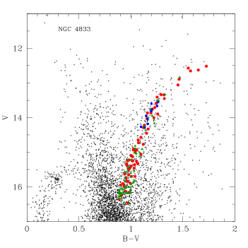
Figure 1: The $V,B-V$ CMD of NGC 4833 (open circles). Stars selected for the present study are plotted as filled, larger symbols: blue squares are the stars observed with UVES, red circles are stars with GIRAFFE spectra, and green triangles are stars observed with GIRAFFE but not analyzed because found to be non members from their RV (see text).

2 Observations

The photometric catalog for NGC 4833 is based on $UBVI$ data (ESO programme 68.D-0265, PI Ortolani), collected at the Wide-Field Imager at the 2.2-m ESO-MPI telescope on 17-21 February 2002. The WFI covers a total field of view of $34^{\prime}\times\leavevmode\nobreak\ 33^{\prime}$, consisting of $8$, $2048\times 4096$ EEV-CCDs with a pixel size of $0\aas@@fstack{\prime\prime}238$. The collected images were dithered in order to cover the gaps between the CCDs, and the exposure times were divided into shallow and deep so as not to saturate the bright red giant stars and, at the same time, sample the faint main sequence stars with a good signal to noise.

The de-biasing and flat-fielding reduction of the CCD mosaic raw images employed the IRAF package MSCRED (Valdes 1998), while the stellar photometry was derived via the use of the DAOPHOT and ALLFRAME programs (Stetson 1994). For specific details of the photometric reduction process see Momany et al. (2004).

The absolute photometric calibration primarily employed the use of $UBVI$ standard stars from Landolt (1992), as well as secondary stars from the Stetson (http://cadcwww.hia.nrc.ca/standards/) library, which provides more numerous and relatively fainter $BVI$ standards. The uncertainties in the absolute flux calibration were of the order of 0.06, 0.03, 0.03, and 0.04 mag, for $UBVI$, respectively. The NGC 4833 catalog was not corrected for sky-concentration, caused by the spurious reflections of light and its subsequent redistribution in the focal plane (Manfroid et al. 2001). As a consequence, photometric comparisons to independent catalogs (based on smaller field of view data) might reveal systematic offsets as a function of the distance from the center of the WFI mosaic.

We selected a pool of stars lying near the RGB ridge line in the colour magnitude diagram (CMD) and without close neighbours, i.e. without any star closer than 3 arcsec (we included also cases with neighbours between 2 and 3 arcsec, but only if fainter by more than 2 mag). The FPOSS tool was used to allocate the FLAMES (Pasquini et al. 2002) fibres.

The stars in our spectroscopic sample are indicated as coloured, filled symbols in Fig. 1. We clearly see that NGC 4833 is heavily contaminated by field stars of the Galactic disk and bulge, given its present location at $l=303.60\deg,\leavevmode\nobreak\ b=-8.02\deg$. Even if the reddening toward the cluster is large and differential (Melbourne& Guhathakurta 2004), thus complicating the analysis, the excision of non-members via radial velocity and the use of infrared filters for temperature determinations as done in similar cases (see e.g. Gratton et al. 2006, 2007), make it feasible.

The log of the observations is given in Table 1. We obtained two exposures with the high resolution GIRAFFE grating and the setup HR11 covering the Na i 5682-88 Å doublet and two exposures with the setup HR13 including the [O i] forbidden lines at 6300-63 Å. Excluding a non-member star and another not useful due to the low S/N of the spectrum, we observed a total of 12 (bright) giants with the fibers feeding the UVES spectrograph (Red Arm, with spectral range from 4800 to 6800 Å and R=47,000, indicated as blue squares in Fig. 1) and 73 with GIRAFFE (seven are in common). The median values of the S/N ratio of spectra obtained with UVES and with the HR11 and HR13 setups of GIRAFFE are 90, 95, and 140, respectively.

Figure 2: Distribution of heliocentric radial velocities (RVs) for stars observed in NGC 4833.

We used the 1-D, wavelength calibrated spectra as reduced by the ESO personnel with the dedicated FLAMES pipelines. Radial velocities (RV) for stars observed with the GIRAFFE spectrograph were obtained using the IRAF task FXCORR, with appropriate templates, while those of the stars observed with UVES were derived with the IRAF task RVIDLINES.

The large RV of NGC 4833 makes it easy to isolate cluster stars from field interlopers. In Fig. 2 we show the histogram of the heliocentric RVs derived for all stars observed; the cluster is easily spotted as a narrow and isolated peak around $V_{r}\simeq 200$ km s^-1. We select as candidate cluster members the 78 stars with $180.0\leq RV\leq$ 220 km s^-1; their membership is fully confirmed by the following chemical analysis, since they all have the same iron abundance, within the uncertainties. The nearest non-member in the velocity space has $RV=141.6\pm 0.7$ km s^-1, $\sim 60$ km s^-1 apart from the systemic velocity of the cluster. A brief overview of the cluster kinematics is provided in Sect. 2.1.

Our optical $B,V$ photometric data were integrated with $K$ band magnitudes from the Point Source Catalogue of 2MASS (Skrutskie et al. 2006) to derive atmospheric parameters as described below, in Section 3.

Coordinates, magnitudes and heliocentric RVs are shown in Table 2 (the full table is only available in electronic form at CDS).

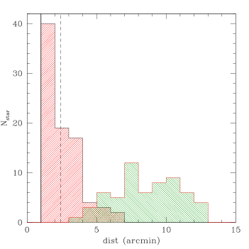
Figure 3: Distribution of observed stars as a function of the radial distance from the centre of NGC 4833. Member stars are indicated in red, while green is used for non members. The solid heavy line indicates the core radius ($r_{c}=1$ arcmin), and the dashed line the half-mass radius ($r_{h}=2.41$ arcmin) from Harris (1996).

Table 1: Log of FLAMES observations for NGC 4833.

Date	UT	exp.	grating	seeing	airmass
		(s)		(”)
Apr. 05, 2009	02:11:37.395	2700	HR11	1.07	1.599
Apr. 05, 2009	02:58:02.303	2700	HR11	1.09	1.519
Apr. 05, 2009	03:54:25.968	2700	HR13	0.64	1.462
Apr. 05, 2009	04:40:47.286	2700	HR13	0.59	1.446

2.1 Radial velocities and kinematics

There is no analysis in the literature dealing with the internal kinematics of NGC 4833, and no estimate of the central velocity dispersion $\sigma_{0}$. It is worth using our sample for a first investigation, albeit it is not especially well suited for this purpose. Indeed our 78 genuine cluster member stars are distributed (see Fig. 3) in the radial range $1.0\leq R/r_{c}\leq 6.6$ or $0.4\leq R/r_{h}\leq 2.8$. Hence we cannot sample the kinematics in the cluster core and in the outer halo (the tidal radius is $r_{t}=17.8r_{c}=7.4r_{h}$, since c=1.25). Our analysis is fully homogenous with that performed in Bellazzini et al. (2012) for the other clusters included in our survey: for further details, we address the interested reader to that paper. The only difference is that here mean velocity and velocity dispersions are estimated with the Maximum Likelihood (ML) procedure described in Martin et al. (2007), that naturally takes into account the effect of errors on the individual RV measures.

First of all we compared the RV estimates obtained from HR13 and HR11 spectra, for the 45 stars that have valid RV measures from both setups. The mean difference for the 35 stars brighter than V=15.5 (i.e. those with the smallest individual errors) is $\langle RV_{13}-RV_{11}\rangle=-0.43\pm 0.07$ km s^-1. This shift was applied to the RV derived from HR11 spectra to bring all the RV estimates to a common zero point. Then, for each star, we adopted the RV estimated from HR13 spectra when present and when the individual uncertainty is lower than the HR11 estimate, and the RV from HR11 in the other cases.

Considering the whole sample of 78 stars we find an average velocity of $\langle RV\rangle=202.0\pm 0.5$ km s^-1 (and a dispersion of $4.1\pm 0.3$ km s^-1), in very good agreement with the value reported by Harris (1996), $\langle RV\rangle=200\pm 1.2$ km s^-1. Fitting a King (1966) model with c=1.25 to the velocity dispersion curve we estimated the central velocity dispersion $\sigma_{0}=5.0\pm 1.0$ km s^-1. We do not find any statistically significant rotation: in the notation of Bellazzini et al. (2012) the rotation amplitude is $A_{rot}=0.9\pm 0.5$ km s^-1 and $A_{rot}/\sigma_{0}=0.18\pm 0.11$. Hence NGC4833 fits excellently into the correlations between metallicity (and horizontal branch morphology) and rotation found by Bellazzini et al., i.e. metal-poor/blue HB clusters tend to have lower rotation than metal-rich/ red HB clusters.

Using the King (1966) formula we estimate a dynamical mass $M_{dyn}=1.3^{+0.6}_{-0.5}\times 10^{5}\leavevmode\nobreak\ M_{\sun}$, and $(M/L)_{V}=0.84\pm 0.45$, on the low side of the range covered by Galactic GCs (see Sollima, Bellazzini & Lee 2012; Pryor & Meylan 1993).

3 Abundance analysis

3.1 Atmospheric parameters

Following our tested procedure, effective temperatures $T_{\rm eff}$ for our targets were derived using an average relation between apparent magnitudes and first-pass temperatures from $V-K$ colours and the calibrations of Alonso et al. (1999, 2001). The rationale behind this adopted procedure is to decrease the star to star errors in abundances due to uncertainties in temperatures, since magnitudes are less affected by measure uncertainties than colours. In the case of NGC 4833, affected by high and variable reddening we used the apparent $K$ magnitudes in our relation with $T_{\rm eff}$ because the impact of the differential reddening on these magnitudes is very limited. This procedure worked very well on other GCs heavily affected by large and differential reddening patterns, like the bulge clusters NGC 6441 (Gratton et al. 2006, 2007) and NGC 6388 (Carretta et al. 2007a). The adopted reddening $E(B-V)=0.32$ mag is from the Harris (1996) catalogue, and it is in perfect agreement with the value derived in the accurate study by Melbourne et al. (2000), who provided an associated error of 0.03 mag. Using Table 3 of Cardelli et al. (1989) this translates into an error of 0.01 mag in $K$ magnitudes that, in turn, corresponds to an uncertainty in temperature of 2.14 K, when coupled to the relation between effective temperature and $K$ magnitude adopted for NGC 4833 in the present study.

Gravities were obtained from apparent magnitudes, assuming the $T_{\rm eff}$’s estimated above, bolometric corrections from Alonso et al. (1999), and the distance modulus for NGC 4833 from Harris (1996). We adopted a mass of 0.85 M_⊙  for all stars and $M_{\rm bol,\odot}=4.75$ as the bolometric magnitude for the Sun, as in our previous studies.

We eliminated trends in the relation between abundances from Fe i lines and expected line strength (Magain 1984) to obtain values of the microturbulent velocity $v_{t}$.

Finally, using the above values we interpolated within the Kurucz (1993) grid of model atmospheres (with the option for overshooting on) to derive the final abundances, adopting for each star the model with the appropriate atmospheric parameters and whose abundances matched those derived from Fe i lines. As discussed in Carretta et al. (2013a) this choise has a minimal impact on the derived abundances with respect to models without overshooting.

3.2 Elemental abundances

Most of our derived abundances rest on analysis of equivalent widths ($EW$). The code ROSA (Gratton 1988) was used as in previous papers to measure $EW$s adopting a relationship between $EW$ and $FWHM$, as described in detail in Bragaglia et al. (2001). Following the approach used in Carretta et al. (2007b) we first corrected the $EW$s from GIRAFFE spectra to the system of the higher resolution UVES spectra, using seven stars observed with both instruments. The correction has the form $EW_{\rm UVES}=0.91(\pm 0.02)\times EW_{\rm GIRAFFE}+1.06(\pm 0.49)$ with an $rms$ scatter of 5.4 mÅ and a Pearson correlation coefficient of $r=0.98$ from 121 lines.

Atomic parameters for the lines falling in the spectral range covered by UVES spectra and by setups HR11 and HR13 in the GIRAFFE spectra are comprehensively discussed in Gratton et al. (2003), together with the adopted solar reference abundances.

Before coadding, each HR13 GIRAFFE spectrum was corrected for blending with telluric lines due in particular to H₂O and O₂ near the forbidden [O i] line at 6300 Å, using synthetic spectra as described in Carretta et al. (2006). Corrections for effects of departures from the LTE assumption according to the descriptions by Gratton et al. (1999) were applied to the derived Na abundances.

We derived abundances of O, Na, Mg, and Si among the elements participating to the network of proton-capture reactions in H-burning at high temperature. Additionally, Al abundances were obtained from the doublet Al i 6696-98 Å for stars observed with UVES.

Beside Mg and Si (numbered among the proto-capture elements), we derived the abundance of the $\alpha-$elements Ca and Ti i; Ti was obtained also from the singly ionized species in stars with UVES spectra. Abundances for the Fe-peak elements Sc ii, V i, Cr i, Cr ii, Mn i, Ni i, and Zn i were also derived, with abundances of some species only obtained for stars with UVES spectra, because of the larger spectral coverage. Corrections due to the hyperfine structure (references in Gratton et al. 2003) were applied to Sc, V, Mn, and Co. Abundances of Cu i were derived from spectrum synthesis, as detailed in Carretta et al. (2011).

The concentration of the neutron-capture elements Y ii, Ba ii, La ii, Nd ii was derived mostly for stars with UVES spectra and mostly from measurements of $EW$s. Results for Y and Ba were checked with synthetic spectra using line lists from D’Orazi et al. (2013) and D’Orazi et al. (2012), respectively. Abundances derived with the two methods are in very good agreement. Lanthanum abundances were obtained from $EW$s of 3-4 lines with transition parameters from Sneden et al. (2003; see also Carretta et al. 2011).

The available Ba lines are all very strong and quite sensitive to the velocity fields in the stellar atmospheres. As a consequence, a clear trend of Ba abundances as a function of the microturbulence results when using the values of $v_{t}$ derived using the weaker Fe lines, formed typically in deeper atmospheric layers (see e.g. Carretta et al. 2013b for a discussion of a similar effect in the analysis of NGC 362). To alleviate this problem, good results are obtained by adopting the values of $v_{t}$ from the relation as a function of the surface gravity provided by Worley et al. (2013) for giants in the metal-poor GC M 15. When analyzed using these values and a constant metallicity equal to the metal abundance derived for NGC 4833 (see next section), no trend is apparent and we can safely explore the Ba abundances looking for intrinsic dispersion or correlations (if any) with other elements. The relation from Worley et al. was chosen since it was shown to efficiently remove any trend between Ba abundances and $v_{t}$ for bright stars in a GC with metallicity comparable to that in NGC 4833. On average, the values of $v_{t}$ from this relation are 0.26 kms^-1 higher than the values derived as described in the previous section for individual stars (with $rms=0.29$ kms^-1, 78 stars). However, for all other species the last method works very well and we adopted for all elements except Ba this approach that guarantees homogeneity with the more than 20 GCs analyzed by our group in this FLAMES survey.

3.3 Metal abundances

The mean metallicity we found for NGC 4833 from stars with high resolution UVES spectra is [Fe/H]$=-2.015\pm 0.004\pm 0.084$ dex ($rms=0.014$ dex, 12 stars) from neutral species, where the first error is from statistics and the second one refers to the systematic effects, as estimated in the next section. From the large sample of stars with GIRAFFE spectra we derived a value of [Fe/H]$=-2.040\pm 0.003\pm 0.073$ dex ($rms=0.024$ dex, 73 stars).

The abundances of iron obtained from the singly ionized species are in excellent agreement with those from neutral lines: [Fe/H]ii$=-2.014$ ($rms=0.021$ dex, 12 stars) from UVES and [Fe/H]ii$=-2.030$ ($rms=0.033$ dex, 59 stars) from GIRAFFE. The derived Fe abundances do not present any trend as a function of the effective temperature, as shown in Fig. 4.

Our average metal abundance seems to be about 0.2-0.3 dex lower than most of previous estimates in literature. From a preliminary analysis of RR Lyrae variables, Murray and Darragh (2013) found [Fe/H]$=-1.67\pm 0.13$ dex using Fourier decomposition of the light curves. We note, however, that often the metallicities based on this method are higher than those derived from high resolution spectroscopy, in particular in the low metallicity regime. For example, [Fe/H]$=-1.98$ dex from RR Lyrae in M 15 (Garcia Lugo et al. 2007), compared to [Fe/H]$=-2.32$ dex from high resolution spectroscopy (Carretta et al. 2009c); [Fe/H]$=-1.23$ dex for M 5 from RR Lyrae (Kaluzny et al. 2000) compared to $-1.34$ (Carretta et al. 2009c); [Fe/H]$=-2.11$ dex from variables in M 30 (Kains et al. 2013), and $-2.34$ from Carretta et al. (2009c). The discrepancy is not limited to our group/analysis: Figuera Jaimes et al. (2013) derived [Fe/H]$=-1.64$ from RR Lyraes in NGC 7492, while Cohen and Melendez (2005) found $-1.82$ dex for this cluster from high resolution spectra. Using high resolution spectra and MARCS models, Kraft and Ivans (2003) found [Fe/H]$=-2.33$ dex and [Fe/H]$=-2.39$ dex for the metal-poor GCs M 30 and M 15, respectively.

From CCD photometry Melbourne et al. (2000) derived a mean metallicity [Fe/H]$=-1.83\pm 0.14$ dex (and a reddening $E(B-V)=0.32\pm 0.03$). Early detections based on high resolution spectra also obtained similar high values: [Fe/H]$=-1.71$ dex from one star (Minniti et al. 1996) and [Fe/H]$=-1.74$ dex, on average, from two stars (Gratton and Ortolani 1989). Moreover, Kraft and Ivans (2003) found for this GC a metallicity [Fe/H]$=-2.06,-2.00,-2.04$ dex from MARCS, and Kurucz models with and without the overshooting option, respectively.

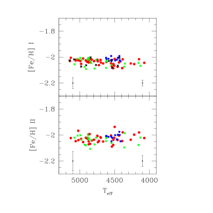
Figure 4: Abundance ratios [Fe/H] i (upper panel) and [Fe/H] ii (lower panel) as a function of T_eff for all analysed stars. Blue squares are stars with UVES spectra, filled circles are those with GIRAFFE spectra observed with both the HR11 and HR13 setups, and crosses indicate stars observed with only the HR11 (black) or the HR13 (green) setup. Error bars on the right and on the left side are star-to-star errors for targets observed with UVES and GIRAFFE, respectively.

3.4 Error budget

Our procedure for error estimates is amply described in Carretta et al. (2007b, 2009a,b) and will not be repeated here. In the following we only provide the main tables of sensitivities of abundance ratios to the adopted errors in the atmospheric parameters and $EW$s and the final estimates of internal and systematic errors for all species analysed from UVES and GIRAFFE spectra of stars in NGC 4833.

The sensitivities of derived abundances on the adopted atmospheric parameters were obtained by repeating our abundance analysis by changing only one atmospheric parameter each time for all stars in NGC 4833 (separately for the UVES and the GIRAFFE samples). The sensitivity in each parameter was adopted as the one corresponding to the average of all the sample.

The amount of the change in the input parameters T_eff, $\log g$, [A/H], and $v_{t}$ to compute the sensitivity of abundances to variations in the atmospheric parameters is shown in the first line of the headers in Table 3 and Table 4, whereas the resulting response in abundance changes of all elements (the sensitivities) are shown in columns from 3 to 6 of these tables.

Table 3: Sensitivities of abundance ratios to variations in the atmospheric parameters, and to errors in the equivalent widths, and errors in abundances for stars of NGC 4833 observed with UVES.

Element	Average	Teff	$\log g$	[A/H]	$v_{t}$	EWs	Total	Total
	n. lines	(K)	(dex)	(dex)	kms-1	(dex)	Internal	Systematic
Variation		50	0.20	0.10	0.10
Internal		4	0.04	0.01	0.10	0.01
Systematic		57	0.06	0.08	0.03
$[$Fe/H$]$i	39	+0.073	$-$0.016	$-$0.015	$-$0.016	0.014	0.022	0.084
$[$Fe/H$]$ii	5	$-$0.017	+0.079	+0.018	$-$0.005	0.038	0.042	0.032
$[$O/Fe$]$i	1	$-$0.050	+0.091	+0.039	+0.014	0.085	0.088	0.090
$[$Na/Fe$]$i	2	$-$0.038	$-$0.030	$-$0.003	+0.011	0.060	0.061	0.096
$[$Mg/Fe$]$i	1	$-$0.029	+0.000	+0.002	+0.011	0.085	0.086	0.072
$[$Al/Fe$]$i	1	$-$0.034	+0.002	+0.003	+0.013	0.085	0.086	0.105
$[$Si/Fe$]$i	4	$-$0.050	+0.025	+0.011	+0.013	0.043	0.045	0.059
$[$Ca/Fe$]$i	15	$-$0.016	$-$0.006	$-$0.003	+0.003	0.022	0.022	0.018
$[$Sc/Fe$]$ii	6	+0.011	$-$0.007	+0.003	+0.011	0.035	0.035	0.029
$[$Ti/Fe$]$i	5	+0.019	$-$0.005	$-$0.002	$-$0.014	0.038	0.040	0.014
$[$Ti/Fe$]$ii	9	+0.025	$-$0.013	$-$0.002	$-$0.002	0.028	0.032	0.023
$[$V/Fe$]$i	2	+0.016	$-$0.006	$-$0.002	+0.013	0.060	0.062	0.019
$[$Cr/Fe$]$i	9	+0.013	$-$0.011	$-$0.007	$-$0.009	0.028	0.030	0.017
$[$Cr/Fe$]$ii	4	$-$0.001	$-$0.011	$-$0.009	+0.000	0.043	0.043	0.013
$[$Mn/Fe$]$i	2	$-$0.012	$-$0.000	+0.001	+0.014	0.060	0.062	0.015
$[$Co/Fe$]$i	1	$-$0.014	+0.001	+0.003	+0.013	0.085	0.086	0.020
$[$Ni/Fe$]$i	8	+0.005	+0.008	+0.003	+0.007	0.030	0.031	0.007
$[$Cu/Fe$]$i	1	+0.010	+0.003	+0.001	+0.010	0.085	0.086	0.021
$[$Zn/Fe$]$i	1	$-$0.075	+0.056	+0.022	$-$0.001	0.085	0.085	0.088
$[$Y/Fe$]$ii	9	+0.031	$-$0.012	+0.000	$-$0.013	0.028	0.031	0.040
$[$Ba/Fe$]$ii	3	+0.043	$-$0.010	+0.002	$-$0.075	0.049	0.090	0.065
$[$La/Fe$]$ii	3	+0.040	$-$0.009	+0.003	+0.001	0.049	0.049	0.046
$[$Nd/Fe$]$ii	4	+0.041	$-$0.009	+0.003	$-$0.000	0.043	0.043	0.048

Table 4: Sensitivities of abundance ratios to variations in the atmospheric parameters and to errors in the equivalent widths, and errors in abundances for stars of NGC 4833 observed with GIRAFFE

Element	Average	Teff	$\log g$	[A/H]	$v_{t}$	EWs	Total	Total
	n. lines	(K)	(dex)	(dex)	kms-1	(dex)	Internal	Systematic
Variation		50	0.20	0.10	0.10
Internal		4	0.04	0.02	0.22	0.02
Systematic		57	0.06	0.07	0.03
$[$Fe/H$]$i	20	+0.064	$-$0.011	$-$0.011	$-$0.016	0.023	0.042	0.073
$[$Fe/H$]$ii	2	$-$0.016	+0.077	+0.011	$-$0.004	0.071	0.074	0.030
$[$O/Fe$]$i	1	$-$0.040	+0.085	+0.031	+0.018	0.101	0.110	0.066
$[$Na/Fe$]$i	2	$-$0.034	$-$0.026	+0.004	+0.013	0.071	0.077	0.055
$[$Mg/Fe$]$i	1	$-$0.027	+0.001	+0.002	+0.013	0.101	0.105	0.039
$[$Si/Fe$]$i	3	$-$0.046	+0.021	+0.009	+0.015	0.058	0.067	0.053
$[$Ca/Fe$]$i	4	$-$0.015	$-$0.006	$-$0.001	+0.001	0.051	0.051	0.017
$[$Sc/Fe$]$ii	4	$-$0.052	+0.082	+0.026	+0.011	0.051	0.059	0.064
$[$Ti/Fe$]$i	3	+0.004	$-$0.004	+0.001	+0.015	0.058	0.067	0.007
$[$V/Fe$]$i	3	+0.021	$-$0.008	$-$0.003	+0.020	0.058	0.073	0.025
$[$Cr/Fe$]$i	1	+0.011	$-$0.006	$-$0.001	+0.021	0.101	0.111	0.018
$[$Co/Fe$]$i	1	$-$0.001	+0.003	+0.005	+0.023	0.101	0.113	0.015
$[$Ni/Fe$]$i	3	$-$0.001	+0.008	+0.004	+0.013	0.058	0.065	0.006
$[$Ba/Fe$]$ii	1	$-$0.033	+0.077	+0.024	$-$0.067	0.101	0.179	0.056

The averages of all measured elements with their $r.m.s.$ scatter are listed in Table 5. Derived atmospheric parameters and Fe abundances for individual stars in NGC 4833 are in Table 6; abundances of proton-capture, $\alpha$-capture, Fe-peak and neutron-capture elements are provided in Tables 7, 8, 9, 10 and 11, respectively. These tables are only available in electronic form: a few lines are given for guidance. Upon request by the referee, we also report in the last two columns of Table 7 the average and rms scatter of the [Na/Fe] ratio in LTE for individual stars, to give an idea of the adopted NLTE corrections.

Table 5: Mean abundances from UVES and GIRAFFE

Element	UVES	GIRAFFE
	n   avg   $rms$	n   avg   $rms$
$[$O/Fe$]$i	12 +0.17 0.22	51 +0.25 0.29
$[$Na/Fe$]$i	12 +0.52 0.29	52 +0.46 0.27
$[$Mg/Fe$]$i	12 +0.27 0.22	44 +0.36 0.15
$[$Al/Fe$]$i	12 +0.90 0.34
$[$Si/Fe$]$i	12 +0.47 0.04	66 +0.46 0.05
$[$Ca/Fe$]$i	12 +0.35 0.01	73 +0.35 0.02
$[$Sc/Fe$]$ii	12 $-$0.04 0.01	73 $-$0.04 0.02
$[$Ti/Fe$]$i	12 +0.18 0.02	53 +0.17 0.02
$[$Ti/Fe$]$ii	12 +0.23 0.01
$[$V/Fe$]$i	12 $-$0.08 0.01	24 $-$0.10 0.02
$[$Cr/Fe$]$i	12 $-$0.24 0.02	24 $-$0.20 0.04
$[$Cr/Fe$]$ii	12 +0.01 0.05
$[$Mn/Fe$]$i	12 $-$0.54 0.01
$[$Fe/H$]$i	12 $-$2.02 0.01	73 $-$2.04 0.02
$[$Fe/H$]$ii	12 $-$2.01 0.02	59 $-$2.03 0.03
$[$Co/Fe$]$i	8 $-$0.03 0.03	7 $-$0.07 0.04
$[$Ni/Fe$]$i	12 $-$0.18 0.01	68 $-$0.18 0.03
$[$Cu/Fe$]$i	12 $-$0.80 0.09
$[$Zn/Fe$]$i	12 +0.07 0.03
$[$Y/Fe$]$ii	12 $-$0.15 0.06
$[$Ba/Fe$]$ii	12 $-$0.06 0.07	62 $-$0.20 0.14
$[$La/Fe$]$ii	12 +0.05 0.03
$[$Nd/Fe$]$ii	12 +0.42 0.04

4 Results

4.1 The Na-O anticorrelation in NGC 4833

After combining the UVES and GIRAFFE datasets and taking into account stars observed with both instruments, we ended with 61 stars with O abundances (40 actual detections and 21 upper limits) and 60 stars with Na abundances. The Na-O anticorrelation in NGC 4833 rests on 51 giants with both O and Na, and is shown in Fig. 5, with star-to-star errors relative to the GIRAFFE dataset. Internal error bars for the UVES sample are slightly smaller (see Table 3).

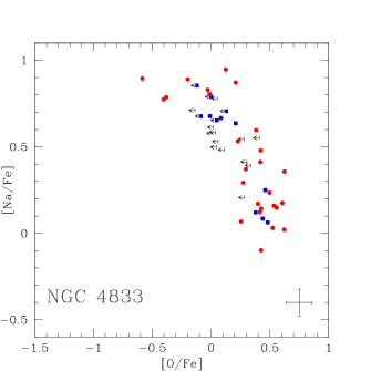
Figure 5: The Na-O anti-correlation observed in NGC 4833. Blue squares are stars observed with UVES, while red circles indicate stars with GIRAFFE spectra. Upper limits in O are shown as arrows, and star-to-star (internal) error bars are plotted.

It is not easy to judge whether stars in NGC 4833 are grouped into discrete populations with homogeneous composition, along the Na-O anticorrelation, mostly formed with the stars observed with GIRAFFE. Similar large samples are better suited to quantify the extension of this feature, but the associated internal errors may smear possible groups, although some sub-divisions are recognizable in Fig. 5. The limited sample of giants observed with UVES seems to be better suited to this task.

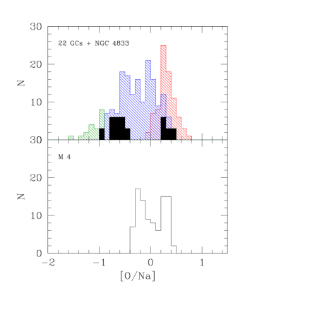
Figure 6: Distribution of the [O/Na] abundance ratios in several GCs from stars observed with the high resolution UVES spectrograph. In the upper panel, about 250 RGB stars in 23 GCs from our FLAMES survey are plotted. Colour coding is red, blue, and green for the P, I, and E components defined in Carretta et al. (2009a). In black we plotted the distribution for NGC 4833 from the present work, with the numbers of stars multiplied by 3 to improve the visibility. Lower panel: distribution of [O/Na] from UVES spectra of about 100 giants in M 4 from Marino et al. (2008).

The 12 stars with UVES spectra are clearly clustered in two clearly separated groups: one with abundances typical of the pattern established by core-collapse supernovae nucleosynthesis (high O and low Na), also shared by field stars of similar metallicity (e.g. Gratton et al. 2000), the other with low-O/high-Na abundances, whose counterparts are rarely observed in Galactic field stars. To check that this occurrence in NGC 4833 is not a spurious effect due to the limited number of giants in the UVES sample, we plotted in Fig. 6 (upper panel) the distribution of the [O/Na] ratios from our total sample of about 250 RGB stars observed with UVES in 22 GCs of the Milky Way in our FLAMES survey. The colour coding corresponds to the division of stars into the primordial (P) component of first generation stars, and to the two fractions of stars with intermediate (I) and extreme (E) composition within the second stellar generation in GCs, as defined in Carretta et al. (2009a) from their location along the Na-O anticorrelation. Our UVES sample in NGC 4833 (shown in Fig. 6 with number counts multiplied by a factor 3 to improve clarity) clearly splits into two groups, roughly coincident with the first and second generation stars. As a comparison, in the lower panel we also plot the only other large sample in an individual GC based on high resolution spectra, the about 100 RGB stars observed in M 4 by Marino et al. (2008). An offset of 0.1 dex was arbitrarily subtracted to their [O/Na] values to bring them on our abundance scale. In M 4, with its short anticorrelation, the extreme component of second generation stars is obviously not present.

Using the quantitative criteria introduced by Carretta et al. (2009a) we can use O and Na abundances to quantify the fraction of the different stellar generations. From the total sample of 51 stars with O and Na we found that the fractions of P, I, and E stars for NGC 4833 are $31\pm 8\%$, $59\pm 11\%$, and $10\pm 4\%$, respectively. The fraction of first generation stars is similar to the one (about one third) typical of the overwhelming majority of Galactic GCs. On the other hand, the fraction of second generation E stars with extremely modified composition is quite large in NGC 4833. As a comparison, the E fraction in GCs like NGC 4590 (M 68), NGC 6809 (M 55), NGC 7078 (M 15), NGC 7099 (M 30), bracketing NGC 4833 in mass and metallicity, does not exceed 2-3% (being formally absent in M 15 and M 68, Carretta et al. 2009a,b). Among the observed RGB stars in NGC 4833 there is apparently no statistically significant segregation in radial distance from the cluster centre for the P, I, and E components. Our sample of member stars is however all confined within two half-mass radii and may be not the optimal sample for this kind of analysis. Large photometric databases are better suited to study possibile difference of radial concentration of different stellar generations.

The interquartile range (IQR) for the ratio [O/Na] is a very useful measurement to quantify the extension of the Na-O anticorrelation (Carretta 2006). From our large sample we found that IQR[O/Na]=0.945 dex in NGC 4833. Therefore, this cluster joins the ensemble of other GCs producing a nice correlation with the cluster total mass (represented by the proxy of the total absolute magnitude, $M_{V}=-8.16$ for NGC 4833 from Harris 1996), established in Carretta et al. (2010a) and reproduced in Fig. 7, left panel. The location of NGC 4833 in this plot seems to be on the upper envelope of the relation defined by the bulk of the other GCs. The position of another cluster sharing a similar position (NGC 288) is also indicated. This occurrence will be discussed in Section 5.

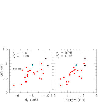
Figure 7: IQR[O/Na] ratios for NGC 4833 (star symbol) and other Galactic GCs as a function of the total cluster absolute magnitude $M_{V}$ (left panel). The other clusters are $\omega$ Cen (filled square, Johnson and Pilachowski 2010), M 54 (filled triangle, Carretta et al. 2010b), and other GCs from our FLAMES survey (filled circles, Carretta et al. 2009a, 2011, 2013b). In the right panel the IQR[O/Na] is shown as a function of the maximum temperature on the horizontal branch, from Recio-Blanco et al. (2006). In each panel, the Spearman rank correlation coefficient ($r_{s}$) and the Pearson’s correlation coefficient ($r_{p}$) are reported.

Recio-Blanco et al. (2006) computed the maximum temperature reached along the horizontal branch (HB) in NGC 4833: $\log T_{\rm eff}=4.301$. The correlation between this parameter and the extension of the Na-O anticorrelation, discovered by Carretta et al. (2007c), is updated and shown in the right panel of Fig. 7. Once again, NGC 4833 seems to lie at the upper envelope of the relation.

4.2 Other proton-capture elements

Apart from the case of O and Na, significant star-to-star abundance variations are detected for other proton-capture elements in giants in NGC 4833. In particular, we found that the [Mg/Fe] abundance ratio shows an unusually large spread in this cluster, with peak-to-peak variations of more than 0.5 dex.

The reality of the intrinsic scatter in Mg is immediately evident comparing the estimated internal error for the UVES sample (0.086 dex) to the observed $rms$ scatter in [Mg/Fe] (0.223 dex): the cosmic spread in Mg among RGB stars in NGC 4833 is significant at almost 3$\sigma$ level.

The run of [Mg/Fe] ratios as a function of the abundance of the proton-capture elements O, Na, and Si is shown in Fig. 8, together with the classical Na-O anticorrelation. The error bars indicate star-to-star errors and are referred to the GIRAFFE sample; internal errors for star of the UVES sample are usually smaller (see Table 3). The Mg abundance is correlated to that of O and anticorrelated with species enhanced in the network of proton-capture reactions, namely Na and Si. We retrieved this pattern from both the datasets observed with UVES and with GIRAFFE.

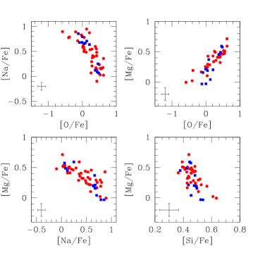
Figure 8: Relations among proton-capture elements O, Na, Mg, and Si in NGC 4833. Red circles refer to stars with GIRAFFE spectra, blue squares indicate stars observed with UVES. The internal errorbars plotted in each panel are those relative to the GIRAFFE sample.

In the case of the GIRAFFE sample, the observed spread in Mg (0.151 dex) does not formally exceed too much the associated internal error (0.105 dex), likely due to the lower resolution of the spectra and the extension of the GIRAFFE sample to warmer giants, with weaker lines. However, even in this case there is no doubt that Mg variations in NGC 4833 are real. In Fig. 9 the HR11 spectra of the two stars with the lowest Mg abundances in the GIRAFFE sample (star 36391, with [Mg/Fe]=+0.02 dex, and star 34613 with [Mg/Fe]=0.00) are compared to the spectra of two other stars with similar atmospheric parameters, but quite different (much higher) Mg abundances.

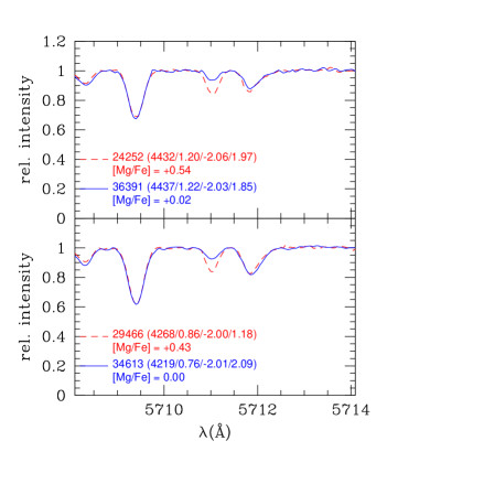
Figure 9: Comparison of two pairs of Mg-poor and Mg-normal stars with similar atmospheric parameters in the Mg i 5711.09 Å spectral region. Atmospheric parameters $T_{\rm eff}$, $\log g$, metallicity, $v_{t}$, and the [Mg/Fe] abundance ratios of stars are indicated in each panel.

This direct comparison, free from any uncertainties related to the abundance analysis, robustly corroborates our findings: there is a large spread in Mg in NGC 4833, where giants with a solar [Mg/Fe] ratio stand side to side with stars having a normal [Mg/Fe] ratio appropriate for metal-poor halo stars.

Large depletions of Mg due to the action of proton-capture reactions in H-burning at high temperature should have two main consequences: produce Al through the Mg-Al cycle and, were the burning temperatures high enough, slightly enhance the abundance of Si through the mechanism of the leakage from the Mg-Al cycle on ²⁸Si (Karakas and Lattanzio 2003).

Abundances of Al can be obtained from the UVES spectra; in four stars out of 12 observed with UVES only upper limits could be derived. Nevertheless, the derived values do not show any trend as a function of the effective temperature and their position reveals instead clear patterns (Fig. 10), with the typical correlations and anticorrelations among elements produced or destroyed, respectively, by the interplay of the Ne-Na and Mg-Al cycles (Denisenkov and Denisenkova 1989, Langer et al. 1993). Moreover, the sample, albeit limited, splits into two clearly separated groups.

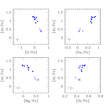
Figure 10: Relations of Al with the proton-capture elements O, Na, Mg, and Si in giants of NGC 4833 observed with UVES spectra. Error bars represent internal errors associated to the UVES sample. The upper limits in Al abundances are indicated by arrows.

The Mg-Si anticorrelation in Fig. 8, together with the Si-Al correlation (Fig. 10), already show that some Si production occurred in the polluters of the first stellar generation in NGC 4833. To further support this evidence, we plot in Fig. 11 the [Si/Fe] ratios as a function of the O and Na values. The evidence of a Si-O anticorrelation is not robust for the GIRAFFE sample, but is clear for the more limited UVES sample. The correlation between Si and Na is well represented in both samples. The two stars with the lowest Mg abundances (Fig. 8 and Fig. 9) are also those showing the highest Si abundances, leaving no doubt that trends in Si and Mg are due to a common mechanism.

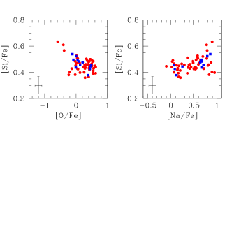
Figure 11: Relations among proton-capture element ratios [Si/Fe], [O/Fe], and [Na/Fe] in NGC 4833. Blue squares indicate stars of the UVES sample, red circles are for stars observed with GIRAFFE. The internal error bars refer to the latter sample.

4.3 Other elements

The pattern of the $\alpha-$elements measured in NGC 4833 is shown as a function of the effective temperatures for indivisual stars in Fig. 12, including also species like Mg and Si involved in the proton-capture reactions discussed in the previous section.

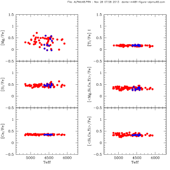
Figure 12: Abundance ratios of $\alpha-$elements Mg, Si, Ca, Ti i as a function of the effective temperature. The average of [$\alpha$/Fe] ratios are shown in the last two panels on the right column (including and excluding the Mg abundance from the mean, respectively). Blue squares are UVES stars. Internal error bars are provided in Tables 3 and  4.

The vertical scale, bracketing the range of [Mg/Fe] ratios, is the same for all the elements to effectively show the large intrinsic dispersion of Mg and, partly, of Si with respect to other $\alpha-$elements with no intrinsic scatter in NGC 4833.

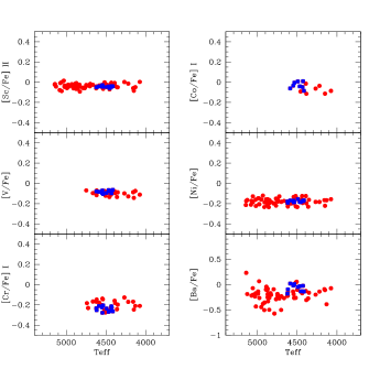
Figure 13: Abundance ratios of elements of the Fe-peak (Sc ii, V, Cr, Co, Ni) and of the neutron-capture element Ba as a function of the effective temperature. Blue squares are UVES stars. Note the different vertical scale for the panel with Ba abundances. Internal error bars are provided in Tables 3 and  4.

The run of elements of the Fe-peak Sc, V, Cr, Co, and Ni as a function of the temperature is shown in Fig. 13 for individual stars in NGC 4833 from the UVES and GIRAFFE samples. These elements present no surprise; they track iron, as in most GCs, with no trend as a function of the $T_{\rm eff}$. The elements Mn and Cu, only available for stars with UVES spectra, show the underabundance typical of metal-poor GCs (e.g. Simmerer et al. 2003, Sobeck et al. 2006).

In the right-bottom panel of Fig. 13 we plot the abundance ratios of Ba, the only neutron-capture element available for a large sample of stars in NGC 4833. As explained in Section 3.2, our finally adopted Ba abundances, displayed in this panel, are those obtained by using for all stars a fixed model metal abundance ([Fe/H]$=-2.02$ dex, the average from the UVES spectra), and the microturbulence from the relation $v_{t}=2.386-0.3067\log g$ derived by Worley et al. (2013) for giants in the metal-poor GC M 15.

As recently shown in Worley et al. (2013) and Carretta et al. (2013a), this approach is quite effective in eliminating any trends of Ba abundances as a function of $v_{t}$ and in reducing the ensueing spurious large scatters of the average. Only for Ba we then adopt these values, our intent being simply to state that this neutron-capture element from $s-$process in NGC 4833 (i) does not have an intrinsic dispersion (compare the $rms$ scatters of the means in Table 5 with the internal errors in Table 3 and 4), and (ii) there is no relation between Ba and elements involved in proton-capture reactions.

We cannot estimate from our data the relative contribution of the $r-$ and $s-$process of neutron capture, because we did not measure a reliable abundance for the typical species that, like Eu, primarily sample an almost pure $r-$process nucleosynthesis at all metal abundances. For the [Ba/Y] ratio we found for NGC 4833 an average value of 0.09 dex ($rms=0.06$ dex, 12 stars) which is perfectly compatible with the ratios of field stars and GCs of similar metallicity (see e.g. Venn et al. 2004).

As for Ba, we found no correlation or anti-correlation whatsoever between the abundances of the $s-$process element La and the abundances of proton-capture elements.

5 Discussion

The Na-O anticorrelation among RGB stars in NGC 4833 reaches a quite long extension. This result must not come unexpected. A statistically robust relation between the extent of the Na-O anticorrelation and the hottest point along the HB is well known (Carretta et al. 2007c, 2010a). On the other hand, the HB in NGC 4833 presents a long blue tail, which stands out clearly, free of field contamination, in particular when high resolution $HST$ imaging is used to construct the CMD (Fig. 14, left panel). Therefore, it would have been easy to predict a long Na-O anticorrelation in this cluster, which is exactly what we found with the current analysis.

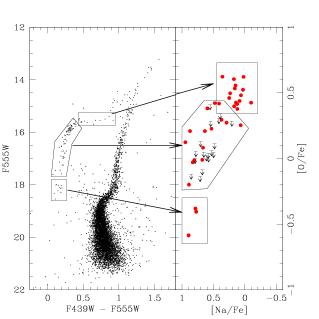
Figure 14: $HST$ colour-magnitude CMD of NGC 4833 from the snapshot survey by Piotto et al. (2002, left): the selected regions along the distribution of HB stars are tentatively associated to different groups along the Na-O anticorrelation from the present work (right panel).

It is tempting to associate the groups selected on the HB in the left panel of Fig. 14 to the RGB stars distributed in the Na-O anticorrelation (right panel of the same figure). After all, RGB stars should end up on the HB after igniting He burning at the centre. Qualitatively, the tentative correspondences illustrated in Fig. 14 may work well, provided that no strong radial gradients are present between our spectroscopic sample and the photometric sample, which cover different parts of the cluster. More quantitative relations must of course await spectroscopic abundance analysis of in situ HB stars.

However, the major peculiarity we uncovered in NGC 4833 is maybe the large spread in Mg, whose abundance is clearly affected by large changes with respect to the usual plateau established by supernovae nucleosynthesis. As discussed in previous sections, we presented proofs that in this cluster also the Si abundance is partially modified by proton-capture reactions. This phenomenon was first observed by Yong et al. (2005) in NGC 6752, another metal-deficient GC with a long blue tail on the HB, and afterward individuated through Si-Al correlations or Si-Mg anticorrelations in a number of other GCs (Carretta et al. 2009b). It is worth noting that in our large FLAMES survey we found significant changes to the Mg (and Si) abundances only in massive and/or metal-poor GCs.

The leakage from the Mg-Al cycle on ²⁸Si puts a strong constraint on the temperature at which H-burning occurred in the stars responsible for polluting the intracluster gas, because the reaction producing ²⁸Si becomes dominant when T${}_{6}\sim 65$ K (Arnould et al. 1999, where the temperature is expressed in millions of Kelvin).

Hence, although this constraint does not allow to discriminate the type of stars providing the raw material for the formation of the second generation (see Prantzos et al. 2007, their figure 8), a logical question is whether NGC 4833 is another case like NGC 2419, although scaled down in amount of the involved elemental variations. In the distant halo cluster NGC 2419, the third most massive GC in our Galaxy, Cohen and Kirby (2012) and Mucciarelli et al. (2012) discovered a double population of stars on the RGB. One group is made of Mg-normal giants with nearly solar abundance of potassium, whereas the other includes stars with a huge depletion of Mg (and large enhancement of K) that apparently do not have a counterpart in any of the other Galactic GCs observed so far concerning K abundances (Carretta et al. 2013c).

In the scenario of multiple populations in GCs, Ventura et al. (2012) advocated that the pattern of abundances observed in NGC 2419 may be explained also by proton-capture reactions occurring in a temperature range much higher than usually observed in more normal cluster stars, favoured by the low metallicity of the cluster. In these particular case, the production of Al from destruction of Mg would be accompanied by the activation of synthesis of heavier elements, such as K, Ca, and also Sc by proton-captures on Ar nuclei. The chief signature of this extreme burning would be the observation of anticorrelations between these elements and Mg, and in NGC 2419 we verified that the hypothesis by Ventura et al. well agrees with observations (Carretta et al. 2013c).

NGC 4833 is far from being as massive as NGC 2419, however we observed clear signature of processing in H-burning at very high temperature in its abundance pattern; moreover it is a metal-poor cluster. We then checked the run of Si, Sc, and Ca as a function of Mg abundances in NGC 4833, but no anticorrelation was found, apart from that between Si and Mg already discussed above. There is only a hint of a correlation between Ca and Sc, that can be intriguing, because formally such a correlation may be expected if both these elements are produced from burning of Mg under the conditions invoked by Ventura et al. (2012). Unfortunately the associated internal errors are large with respect to the amount of the variations and the correlation is scarcely statistically significant (the Pearson correlation coefficient is only 0.25; with a number of degrees of freedom exceeding 70 this implies that the correlation is significant only at about 95-98% in two-tail tests).

Therefore, NGC 4833 cannot be considered a true sibling of NGC 2419, that still continues to represent an $unicum$ among GCs. Nevertheless, we found in the present study that NGC 4833, with its associated extreme chemistry, stands out among other globular clusters. To illustrate this finding we used the [Ca/Mg] vs [Ca/H] plane adopted in Carretta et al. (2013c) as a diagnostic for the relevance of the high temperature nuclear cycles possibly activated in polluters of the first generation in GCs. While measurements of the K abundance are still scarce, Ca and Mg are measured for a large number of stars, providing the precious advantage of good statistics.

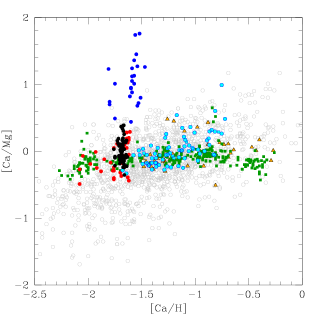
Figure 15: The [Ca/Mg] ratio as a function of the Ca abundances for several stellar populations, adapted from Carretta et al. (2013c). Grey open circles are stars in eight dwarf spheroidal Milky Way satellite galaxies (Kirby et al. 2011); blue and red filled circles are RGB stars in NGC 2419 with [Mg/Fe] lower and larger than 0.0 dex, respectively, from Cohen and Kirby (2012) and Mucciarelli et al. (2012). Orange triangles are giants in $\omega$ Cen (Norris and Da Costa 1995), cyan circles are RGB stars in M 54 (Carretta et al. 2010b). Green squares are for giants in 22 Galactic GCs (Carretta et al. 2009b, 2010c, 2011, 2013a,b). Black symbols are stars in NGC 4833 from the present study (squares and circles for the UVES and GIRAFFE samples, respectively).

In Fig. 15 we updated this diagnostic plot by adding stars of NGC 4833 analyzed in the present paper. Typically, the [Ca/Mg] ratios in GC stars show small spread over a range of about 2 dex in Ca, with a few exceptions, represented by few giants in $\omega$ Cen and M 54, the two most massive clusters in the Galaxy, considered to be the nuclei left from dwarf galaxies accreted in the past. The three Mg-poor stars in NGC 2808 (Carretta et al. 2009b) stand out around [Ca/H]$\sim-0.85$ dex, while in the low metallicity regime the stars of NGC 4833 show a large dispersion in [Ca/Mg] when compared to other GCs. The spread in NGC 4833 does not reach the high values of the peculiar Mg-poor component in NGC 2419, however the stars in NGC 4833 with the largest depletion in Mg reach the same level of the most Mg-poor stars in $\omega$ Cen. We caution the reader that among GCs stars small offsets could exist with respect to the samples by Cohen and Kirby, Mucciarelli et al. and Norris and Da Costa, whereas all other RGB stars are from the homogeneous analysis by our group. There is no doubt that NGC 4833 shares some of the peculiarities also seen in $\omega$ Cen, M 54 and NGC 2808, although all these GCs are far from reaching the huge Mg-depletions observed in NGC 2419.

All these objects are high mass clusters, while the extension of the HB and of the Na-O anticorrelation (and, overall, of the proton-capture processing) are quite large in NGC 4833 with respect to its absolute magnitude. Hence, we could wonder about the reason why NGC 4833 is not so massive,

In Fig. 7 we indicated the position of NGC 288 in the relation between the extension of the Na-O anticorrelation and total cluster mass (luminosity). In Carretta et al. (2010a) we discussed the evidence that GCs lying on the left of this relation lost a larger than average fraction of their mass after their formation. This conclusion stemmed from old, classical proofs (like tidal tails associated to NGC 288, Leon et al. 2000) or from new interpretation of independent observations (like the number density of X-ray sources in M 71, see Section 5.3 in Carretta et al. 2010a).

Are there any indication of a huge mass loss also in NGC 4833? The field of view around NGC 4833 is very crowded (see Fig. 1), with variable reddening, and probably this deterred investigations looking for tidal tails around GCs, because we are not aware of any studies of this kind for NGC 4833.

Another approach could be to look for clues from the present-day mass function (PDMF). Unfortunately, there seems to be no determination of the PDMF for NGC 4833, again probably bacause of the difficulties related to the above mentioned conditions. We note that GCs with central brightness $\mu_{V}$, concentration, and central density $\rho_{0}$ similar to those of NGC 4833 present a PDMF with a rather steep slope of about -1 (de Marchi and Pulone 2007, Paust et al. 2010), indicating many low mass stars, and therefore little evidence of mass loss.

However, these other GCs are characterised by less critical orbits. Dynamical considerations suggest that NGC 4833 could actually be in a phase of destruction because of the tidal interaction with the bulge of the Galaxy. The concentration of NGC 4833 is modest (c=1.25, Harris 1996) and it is worth noting that the cluster has a very eccentric orbit ($e\sim 0.84$; Casetti-Dinescu et al. 2007) passing very close to the Galactic bulge. This is probably a lethal combination, for a cluster.

We inserted the data for NGC 4833 (from Harris 1996 and Casetti-Dinescu et al. 2007) in the equation 2 of Dinescu et al. (1999) that estimates the inverse ratio of the destruction time due to bulge shocking. For NGC 4833 we derived a destruction time between 1 and 3$\times 10^{8}$ years. The exact value depend on the mass of the Galactic bulge, assumed to be 34$\times 10^{9}$ $M_{\odot}$ (Johnston et al. 1995), and on the velocity at the pericentre of the orbit, between 200 and 400 km s^-1. The estimate may increase by a factor 2.5 by adopting a pericentre distance of 0.9 kpc, at the upper boundary of the range considered by Casetti-Dinescu et al. (2007), instead of 0.7 kpc. When compared to the other GCs included in the sample of Dinescu et al. (1999), NGC 4833 show particularly critical parameters, and therefore it is a good candidate to strong tidal stripping and destruction by the bulge. Our estimate is approximate, but these findings are supported by Allen et al. (2006, 2008), who found that NGC 4833 has the sixth larger destruction rate among the 54 GCs analysed by them.

Incidentally, the low value of the $(M/L)_{V}$ we found (Section 2.1) also supports the hint of a significant loss of stars from the cluster, since energy equipartition should have favored the loss of low mass stars.

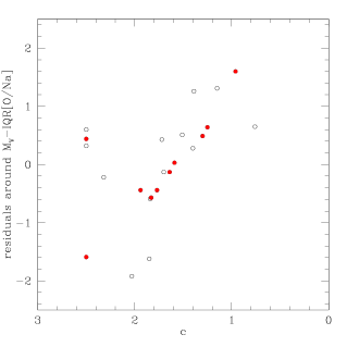
Figure 16: Residuals around the relation between total absolute cluster magnitude $M_{V}$ and the interquartile range IQR[O/Na] as a function of the cluster concentration $c$ for GCs from our FLAMES survey. Filled points indicate inner halo clusters, as defined in Carretta et al. (2010a).

The location of NGC 4833 and NGC 288 on the $M_{V}-IQR$ diagram suggests that variations in cluster concentration $c$ can at least in part explain the observed scatter. In Fig. 16 we plotted the residuals around the $M_{V}-IQR$ correlation against the cluster concentration $c$: there is indeed a significant anti-correlation between these two quantities: the Pearson linear correlation coefficient is $r_{p}=0.52$ that has a probability lower than 1% to be a random result. Of course, in this case it is better to use a bivariate analysis; the best fit is then:

$$IQR=-0.16-(0.14\pm 0.04)M_{V}-(0.16\pm 0.08)c.$$ (1)

The r.m.s. of residuals around this regression is 0.18, which compares well with typical internal errors in IQR[O/Na]. The correlation would further improve by excluding the core-collapse GCs, whose concentration is arbitrarily put at the constant value 2.5 in Harris (1996). The Pearson linear coefficient provided by this regression is $r_{p}=0.65$. This result indicates that at a given absolute magnitude $M_{V}$, more loose clusters have a more extended Na-O anticorrelation than more compact ones. This might seem in contradiction with the observation that second generation stars are more centrally concentrated than first generation ones, at least in several clusters (Gratton et al. 2012 and references therein). However, it may well be explained if the real parameter driving the Na-O anticorrelation is the original rather than the present day mass, and more loosely concentrated clusters lost more mass than the more compact ones. Hence, the original mass of loosely concentrated clusters is on average larger than that of more compact clusters that now have the same $M_{V}$. More loose clusters are actually expected to be destroyed at a much faster rate by the tidal effects of the bulge and disk because the destruction rates for these mechanisms are expected to be proportional to the inverse of the cluster density (see eqs. (1) and (2) in Dinescu et al. 1999).

Note that if this argument is correct, IQR[O/Na] could be considered a better proxy to the original cluster mass than $M_{V}$. We might then possibly use the location of a cluster in the $M_{V}-IQR$ diagram not only to infer its original mass, but also the amount of mass lost (assuming that very compact clusters loose only a small fraction of their original mass). This is a quite speculative but interesting possibility, that should be compared with other dynamical indicators of mass loss, like e.g. the slope of the mass function. We intend to make such a comparison in a future study.

6 Summary

In the extension of our FLAMES survey of Na-O anticorrelation in GCs (e.g. Carretta et al. 2009a,b), we analyzed FLAMES data for 78 RGB member stars of NGC 4833 (73 observed with GIRAFFE, 12 with UVES, of which seven in common). This is the first massive high-resolution spectroscopic study of this cluster. We confirmed that it is a metal-poor GCs, with an average [Fe/H]=$-2.04\pm 0.003$ from the 73 GIRAFFE stars and $=-2.015\pm 0.004$ from the 12 UVES stars. The $rms$ dispersion is very small (0.024 and 0.014 dex, respectively), making NGC 4833 one of the most homogenous GC, at least in its general metallicity.

We obtained abundances of Na and O and we concluded that the cluster presents the typical Na-O anticorrelation found in (almost) all MW GCs (e.g., Carretta et al. 2010a, Gratton et al. 2012). The extension of the anticorrelation, as measured from the interquartile range of the [O/Na] ratio, is large. This is in line with the expectations based on its very extended HB. The limited sample of UVES stars shows a marked bimodality in Na and O abundances, as well as in Mg, Al, Si, with P and I,E stars clearly separated. The GIRAFFE sample shows only a hint of this separation, because of the larger errors in the abundances.

More exceptional is however the finding of large star-to-star variation in Mg abundance, anticorrelated with Al, Na, and Si. The strong depletion in Mg implies nuclear processing at very high temeperatures, exceeding a threshold equal to about 65 million of Kelvin (Arnould et al. 1999). This has been found to date only in a few cases, mostly metal-poor and/or massive GCs, with the more extreme changes seen in objects such as the very massive $\omega$ Cen, M 54, and NGC 2419 (and in a smaller degree in NGC 2808). NGC 2419, with a metallicity similar to NGC 4833, is a more extreme case and clearly a unicum among GCs in the Milky Way. However, NGC 4833 reaches Mg depletion similar to the other massive clusters mentioned above and it stands out among GCs of similar low metallicity.

This unusual chemical pattern, coupled with the position of NGC 4833 in the relation between IQR[O/Na] and mass (total absolute magnitude), seems to indicate that the cluster was much more massive in the past. NGC 4833 has probably lost a conpicuous fraction of its original mass due to bulge shocking, as also indicated by its orbit.

Table 2: List and relevant information for target stars in NGC 4833 The complete Table is available electronically only at CDS.

ID	RA	Dec	$B$	$V$	$K$	RV(Hel)	Notes
22810	12 59 5.559	-70 56 59.87	16.470	15.491	12.337	198.79	HR11,HR13
23306	12 58 49.698	-70 55 17.19	16.736	15.696	12.439	205.33	HR11,HR13
23437	12 58 54.862	-70 54 59.07	16.153	15.056	11.711	195.26	HR11
23491	12 59 5.197	-70 54 53.86	14.242	12.516	8.270	200.33	HR11,HR13
23518	12 59 12.686	-70 54 50.03	16.395	15.359	12.206	203.73	HR13
24063	12 58 54.127	-70 53 46.86	14.660	13.343	9.651	203.13	HR13
24252	12 59 16.083	-70 53 28.91	14.916	13.663	10.046	202.26	UVES

Table 6: Adopted atmospheric parameters and derived iron abundances. The complete table is available electronically only at CDS.

Star	$T_{\rm eff}$	$\log$ $g$	[A/H]	$v_{t}$	nr	[Fe/H]i	$rms$	nr	[Fe/Hii	$rms$
	(K)	(dex)	(dex)	(km s-1)		(dex)			(dex)
22810	4893	2.17	$-$2.04	1.46	23	$-$2.037	0.118	2	$-$2.027	0.115
23306	4914	2.20	$-$2.03	1.44	21	$-$2.026	0.140	1	$-$2.021
23437	4767	1.89	$-$2.06	1.19	5	$-$2.061	0.062
23491	4074	0.45	$-$2.04	2.07	38	$-$2.044	0.105	3	$-$2.023	0.037
23518	4867	2.12	$-$2.02	1.43	20	$-$2.017	0.101	2	$-$2.024	0.001
24063	4352	1.04	$-$2.05	1.88	26	$-$2.050	0.090	2	$-$1.985	0.005
24252	4432	1.20	$-$1.99	1.88	38	$-$1.992	0.058	5	$-$1.975	0.040

Table 7: Abundances of proton-capture elements in stars of NGC 4833. n is the number of lines used in the analysis. Upper limits (limO,Al=0) and detections (=1) for O and Al are flagged.

star	n	[O/Fe]	rms	n	[Na/Fe]	rms	n	[Mg/Fe]	rms	n	[Al/Fe]	rms	limO	limAl	[Na/Fe]LTE	rms
22810	1	+0.23		3	+0.53	0.04	1	+0.34					1		+0.49	0.05
23306	1	+0.62		2	+0.36	0.10	2	+0.59	0.03				1		+0.28	0.11
23437				2	+0.36	0.03	1	+0.39					1		+0.22	0.03
23491	1	$-$0.01		3	+0.80	0.05	2	+0.25	0.02				1		+0.38	0.05
23518	1	+0.55					1	+0.47					1
24063	2	$-$0.20	0.03	2	+0.89	0.00							1		+0.58	0.00
24252	1	+0.48		2	+0.06	0.02	1	+0.58		1	+0.43		1	0	$-$0.12	0.02

Table 8: Abundances of $\alpha$-elements in stars of NGC 4833. n is the number of lines used in the analysis.

star	n	[Si/Fe]	rms	n	[Ca/Fe]	rms	n	[Ti/Fe] i	rms	n	[Ti/Fe] ii	rms
22810	6	+0.44	0.22	4	+0.36	0.05	1	+0.19
23306	2	+0.39	0.01	6	+0.35	0.09	2	+0.17	0.09
23437	2	+0.51	0.06	1	+0.31
23491	6	+0.45	0.14	5	+0.34	0.12	4	+0.15	0.05
23518	1	+0.41		3	+0.38	0.02	1	+0.17
24063	1	+0.40		5	+0.37	0.05	3	+0.17	0.01
24252	5	+0.45	0.06	13	+0.35	0.05	7	+0.17	0.06	8	+0.22	0.04

Table 9: Abundances of Fe-peak elements in stars of NGC 4833. n is the number of lines used in the analysis.

star	n	[Sc/Fe] ii rms	n	[V/Fe] rms	n	[Cr/Fe] i rms	n	[Cr/Fe] ii rms	n	[Mn/Fe] rms	n	[Co/Fe] rms	n	[Ni/Fe] rms	n	[Cu/Fe] rms	n	[Zn/Fe] i rms
22810	4	-0.04 0.09											3	-0.16 0.27
23306	5	-0.03 0.24											2	-0.23 0.19
23437	5	-0.06 0.06											2	-0.15 0.18
23491	6	+0.00 0.04	4	-0.11 0.03	2	-0.21 0.10					1	-0.09	6	-0.16 0.11
23518	1	-0.03											2	-0.19 0.06
24063	2	-0.05 0.08	2	-0.09 0.05	1	-0.20							3	-0.16 0.06
24252	8	-0.05 0.14	4	-0.10 0.01	12	-0.21 0.07	6	+0.01 0.08	2	-0.54 0.08	1	-0.05	9	-0.17 0.07	1	-0.85	1	+0.04

Table 10: Abundances of $n-$capture elements in stars of NGC 4833 with UVES spectra; n is the number of lines used in the analysis.

star	n	[Y/Fe] ii	rms	n	[La/Fe] ii	rms	n	[Nd/Fe] ii	rms
24081	10	$-$0.15	0.11	4	+0.30	0.16	4	+0.45	0.09
24252	6	$-$0.24	0.07	5	+0.35	0.12	4	+0.47	0.05
31163	10	$-$0.11	0.08	3	+0.25	0.07	4	+0.36	0.10
31332	10	$-$0.09	0.10	4	+0.40	0.13	4	+0.39	0.11
33347	9	$-$0.19	0.09	3	+0.30	0.04	4	+0.44	0.10
33554	10	$-$0.13	0.09	4	+0.25	0.15	4	+0.42	0.09
35680	5	$-$0.09	0.06	3	+0.35	0.06	4	+0.40	0.11
36402	7	$-$0.24	0.09	2	+0.25	0.22	3	+0.44	0.04
36454	9	$-$0.16	0.13	3	+0.25	0.11	3	+0.36	0.07
36484	9	$-$0.12	0.09	3	+0.40	0.06	4	+0.41	0.13
37197	9	$-$0.23	0.14	2	+0.50	0.05	3	+0.40	0.15
37498	9	$-$0.10	0.10	4	+0.25	0.07	4	+0.46	0.07

Table 11: Abundances of Ba ii in stars of NGC 4833. n is the number of lines used in the analysis.

star	n	[Ba/Fe]ii	rms
22810	1	$-$0.10
23306	1	$-$0.50
23437
23491	1	$-$0.07
23518	1	$-$0.33
24063	1	$-$0.16
24252	3	$-$0.13	0.01