How Best to Handle a Dicey Situation

Abstract

We introduce the Destructive Object Handling (DOH) problem, which models aspects of many real-world allocation problems, such as shipping explosive munitions, scheduling processes in a cluster with fragile nodes, re-using passwords across multiple websites, and quarantining patients during a disease outbreak. In these problems, objects must be assigned to handlers, but each object has a probability of destroying itself and all the other objects allocated to the same handler. The goal is to maximize the expected value of the objects handled successfully.

We show that finding the optimal allocation is $\mathsf{NP}$-$\mathsf{complete}$, even if all the handlers are identical. We present an FPTAS when the number of handlers is constant. We note in passing that the same technique also yields a first FPTAS for the weapons-target allocation problem [1] with a constant number of targets. We study the structure of DOH problems and find that they have a sort of phase transition – in some instances it is better to spread risk evenly among the handlers, in others, one handler should be used as a “sacrificial lamb”. We show that the problem is solvable in polynomial time if the destruction probabilities depend only on the handler to which an object is assigned; if all the handlers are identical and the objects all have the same value; or if each handler can be assigned at most one object. Finally, we empirically evaluate several heuristics based on a combination of greedy and genetic algorithms. The proposed heuristics return fairly high quality solutions to very large problem instances (upto 250 objects and 100 handlers) in tens of seconds.

1 Introduction

Consider the problem of transporting multiple types of explosives across a war-zone when multiple options of transportation are available (eg., armoured trucks, naval carriers, submarines, transport aircrafts, etc). Each transportation option has a non-negligible probability of being destroyed by enemy combatants or by the mishandling of (possibly faulty) explosives. The goal is to find an allocation of explosives to transportation units such that expected value of delivered explosives is maximized. We classify such allocation problems as Destructive Object Handling (DOH) problems.

Formally, a DOH problem consists of a set of $n$ objects that must be allocated to $k$ handlers. For $j=1,\dots,n$, the $j^{th}$ object has value $v_{j}$ and a vector of non-self-destruction probabilities $\langle p_{1j},\dots,p_{kj}\rangle$. Here, $p_{ij}$ denotes the probability that the $j^{th}$ object will not self-destruct if allocated to the $i^{th}$ handler. All the objects allocated to a handler survive if none of them self-destruct, otherwise they are all lost. Self-destruction probabilities are assumed to be independent. The goal is to find an allocation that maximizes the expected value of surviving objects.

Problem 1

The Generic Destructive Object Handling (DOH) problem. Given $v_{1},\dots,v_{n}$ and $p_{ij}$ for $i=1,\dots k$ and $j=1\dots,n$, find partition $S_{1}\cup\dots\cup S_{k}$ of $\{1,\dots,n\}$ that maximizes $ES=\sum_{i=1}^{k}ES_{i}$, where $ES_{i}=\sum_{j\in S_{i}}v_{j}\prod_{j\in S_{i}}p_{ij}$.

We will use the notation $V_{i}=\sum_{j\in S_{i}}v_{j}$ and $P_{i}=\prod_{j\in S_{i}}p_{ij}$, so $ES=\sum_{i=1}^{k}ES_{i}=\sum_{i=1}^{k}P_{i}V_{i}$. Note that the DOH problem can also model values for handlers and allocation-independent destruction probabilities by creating proxy objects corresponding to each handler. In addition to hazardous object shipping, DOH problems arise in many other real world contexts.

Emergency quarantine. During an outbreak of a disease with a short incubation period, medical staff may need to quarantine patients collectively, i.e. patients may be sealed in multiple rooms for the incubation duration. If no one in a room is infected, then all the patients in that room survive and are released. If any one of the patients in a room is sick, then all the patients in that room are, sadly, lost. Given an initial estimate of the probability that a patient is sick based on physical observations, such as fever, cuts, bite marks, etc., how should staff assign patients to rooms to maximize the expected number survival rate?

Process allocation with marginal nodes. Large computing clusters may have nodes that are marginal, i.e. they sometimes crash due to faulty RAM, overheating, etc., and the probability that a node crashes may depend on the number and kind of processes allocated it. Assuming no checkpointing, if a node crashes, then all the work it has performed is lost. Given a value for each task, and probabilities $q_{ij}$ that task $j$ will crash machine $i$, how should processes be allocated to machines so as to maximize the expected value of completed tasks?

Re-using passwords. Recent studies show that humans, on average, distribute six passwords amongst 25 web service accounts [2]. If an attacker manages to steal the password database for one of these services [3] and recovers the user’s password for that service, then, due to the strong linkability [4] of web based accounts, he can easily break into all the other accounts that share that password. If the user’s $i^{th}$ password is assigned to her $j^{th}$ account, then the probability, $q_{ij}$, that an attacker obtains the $i^{th}$ password by breaking into the $j^{th}$ web service is a function of (1) the security of the $j^{th}$ web service, and (2) the strength of the $i^{th}$ the password (but only if the $j^{th}$ service stores password hashes instead of passwords [5]). Thus, given estimates of the value of each account, the security of each service provider, the strength of each password, and whether each service provider stores passwords or hashes, we can ask: how should a user allocate accounts to passwords so as to minimize her expected loss from server breakins?

		Approximation Results
Problems	Class	Factor	Time Complexity
General DOH problem (Sections 2, 3.2)	at least $weakly$ $\mathsf{NP}$-$\mathsf{C}$	$\frac{(1-\epsilon)(c-1)}{k}$	$O(\frac{k^{c}n^{2c+1}\ln^{c}P\ln^{c}V}{\epsilon^{2c}})$
DOH with $k=O(1)$ (Sections 2, 3)	$weakly$ $\mathsf{NP}$-$\mathsf{C}$	$1-\epsilon$	$O(\frac{n^{2k+1}\ln^{k}V\ln^{k}P}{\epsilon^{2k}})$
Identical Handlers (Section 2)	at least $weakly$ $\mathsf{NP}$-$\mathsf{C}$	Same as General DOH	Same as General DOH
Identical Values	Open	Same as General DOH	Same as General DOH
Identical Objects (Section 4.1)	$\mathsf{P}$	1	$O(nk)$
Identical Handlers and Values (Section 4.2)	$\mathsf{P}$	1	$O(n^{2}k)$
Identical Risks (Section 4.3)	$\mathsf{P}$	1	$O(n^{2}k)$
At most one object per handler (Section 4.5)	$\mathsf{P}$	1	$O\left(n^{3}k\log n\right)$

Table 1: Summary of Complexity Results. Here, $k$ is the number of handlers, $n$ is the number of objects, $P=\min(\prod_{j=1}^{n}p_{1j},\dots,\prod_{j=1}^{n}p_{kj})$, and $V=\min_{j}v_{j}/\sum_{j=1}^{n}v_{j}$.

1.1 Contributions and Organization

A summary of theoretical results presented in this paper is shown in Table 1. In Section 2, we show that the DOH problem is NP-complete, even if all the handlers are identical. We provide an FPTAS for the DOH problem when the number of handlers is a constant in Section 3. Coincidentally, the same technique also yields the first FPTAS for the Weapons-Target Allocation problem with a constant number of targets. In Section 4, we provide polynomial time algorithms for the following special cases: when the survival probabilities depend only on the handler, when all objects have the same values and all handlers are identical, when all the objects are identical, and when at most one object can be allocated to each handler. Heuristic approaches for finding allocations are proposed and compared in section 5. Finally, we summarize our conclusions.

1.2 Related Work

In terms of similarity of objective functions, the DOH problem is most closely related to the static Weapon-Target Allocation problem (WTA). The WTA problem [1] is a well studied non-linear allocation problem in the field of command-and-control theory in which the objective is to allocate missiles to enemy locations so as to inflict maximum damage (given that each missile $j$ destroys a target $i$ with probability $p_{ij}$). The problem was shown to be at least weakly $\mathsf{NP}$-$\mathsf{Complete}$ by Lloyd and Witsenhausen [6] . We show in this paper that, when the number of targets is constant, the problem admits an FPTAS. While certain similarities exist between the WTA objective function ($F_{wta}=\sum_{i=1}^{k}\prod_{j\in S_{i}}p_{ij}$) and the DOH objective function (Problem 1), a major complicating difference is the absence of an additive sub-component to $F_{wta}$. As a result, unlike the WTA problem, the objective function of the DOH problem does not yield a convex function even after relaxation of the integer requirement.

The DOH problem has many applications in the domain of hazardous material processing and routing [7]. These problems generally deal with the selection of minimum risk processing locations [8] and transportation routes in networks [9], [10] – i.e., finding minimum cost facility locations and routes for which human and external material loss in the event of malfunction incidents is minimized.

2 Complexity of DOH Problems

In this section, we show that the DOH problem is at least weakly $\mathsf{NP}$-$\mathsf{Complete}$.

Definition 1

Decisional DOH Problem (D-DOH): Given a DOH problem and a threshold $r$, does there exist an allocation such that $ES\geq r$?

Theorem 2.1

$D$-DOH problems are at-least weakly $\mathsf{NP}$-$\mathsf{Complete}$.

Proof

Membership in $\mathsf{NP}$ is easily established. Given a guess for $S_{1},\dots,S_{k}$, we just compute $ES$ and verify that it is at least $r$. This can be done in time proportional to the length of the words representing the values and probabilities.

We will reduce the well studied $3$-$Partition$ problem ($3P$) as defined in [11], to the $D$-DOH problem. Given an instance $I_{3P}:X=\{x_{1},\dots,x_{3n}\}$ (where $\sum_{j=1}^{3n}x_{j}=nB$) of the $3P$ problem, we create an instance $I_{DOH}$ of the $D$-DOH problem with $3n$ objects and $n$ handlers as follows:

• Pick a rational number $b\in(1,e^{4/nB})$.

• Set $v_{j}=x_{j}$, $\forall j\in\{1,\dots,3n\}$.

• Set $p_{ij}=b^{-x_{j}}$, $\forall j\in\{1,\dots,3n\}$ and $\forall i\in\{1,\dots,n\}$.

• Set $r=n\times B\times b^{-B}$.

By construction, $\sum_{i=1}^{n}V_{i}=nB$ and, for any allocation $S_{1},\ldots,S_{n}$, we have $ES=\sum_{i=1}^{n}V_{i}b^{-V_{i}}$. We now argue that, because of the choice of the base, $b$, $ES\leq\sum_{i=1}^{n}Bb^{-B}=r$. Consider any unequal allocation, i.e. in which there exist $i$ and $i^{\prime}$ such that $V_{i}\not=V_{i^{\prime}}$. We will show that the allocation would be improved by redistributing the value equally between handlers $i$ and $i^{\prime}$. Consider the function $f(x)=xb^{-x}+(c-x)b^{-(c-x)}$, where $c=V_{i}+V_{i^{\prime}}\leq nB$. First, observe that $f^{\prime}(c/2)=0$. Second, since $b<e^{4/c}$, $f^{\prime}(x)>0$ for all $x\in[0,c/2)$ and $f^{\prime}(x)<0$ for $x\in(c/2,c]$. Hence $x=c/2$ is a global maximum. Thus, if an allocation has any $i,i^{\prime}$ such that $V_{i}\not=V_{i^{\prime}}$, we could improve it by replacing $V_{i}$ and $V_{i^{\prime}}$ by $(V_{i}+V_{i^{\prime}})/2$. Hence the optimal allocation must have $ES\leq\sum_{i=1}^{n}Bb^{-B}=r$, and this can only be obtained if $V_{1}=\dots=V_{n}=B$.

Therefore, if there is a solution to the 3P problem, then there exists an allocation for the D-DOH problem in which $V_{1}=\dots=V_{n}=B$, so that $ES=r$. If, on the other hand, there is an allocation of the D-DOH problem such that $ES\geq r$, then we must have $ES=r$ and $V_{1}=\dots=V_{n}=B$, so there exists a solution to the original 3P problem.

Theorem 2.1 shows that even the restricted D-DOH problem – where probabilities are object dependent but handler independent – is weakly $\mathsf{NP}$-$\mathsf{Complete}$. It remains an open question whether the D-DOH problem is strongly $\mathsf{NP}$-$\mathsf{Complete}$.

3 Boundable Approximations

We now derive an approximation algorithm for the DOH problem. The algorithm, which is based on dynamic programming with state-space trimming [12], is an FPTAS when $k=O(1)$. We then build on this result and present an approximation for arbitrary $k$ in Section 3.2.

Consider allocating the objects to handlers one at a time, i.e. we allocate the first object, then the second, etc. Let $S_{ti}$ be the set of objects allocated to the $i^{th}$ handler at time step $t$, $V_{ti}=\sum_{j\in S_{ti}}v_{j}$, and $P_{ti}=\prod_{j\in S_{ti}}p_{ij}$, $ES_{ti}=P_{ti}V_{ti}$, and $ES_{t}=\sum_{i=1}^{k}ES_{ti}=\sum_{i=1}^{k}P_{ti}V_{ti}$. If we allocate the $t+1$st object to the $\ell$th handler, then we will have

$$\begin{array}[]{lcr}P_{t+1,i}=\left\{\begin{array}[]{ll}P_{t,i}p_{\ell,t+1}&\textrm{ if }i=\ell\\ P_{t,i}&\textrm{ if }i\not=\ell\end{array}\right.&&V_{t+1,i}=\left\{\begin{array}[]{ll}V_{t,i}+v_{\ell,t+1}&\textrm{ if }i=\ell\\ V_{t,i}&\textrm{ if }i\not=\ell\end{array}\right.\end{array}$$

Thus $(V_{t1},\dots,V_{tk},P_{t1},\dots,P_{tk})$ is the only state information we need to compute the state after allocating the $t$’th object. This also gives a dominance relation among allocations: if $V_{ti}\leq V^{\prime}_{ti}$ and $P_{ti}\leq P^{\prime}_{ti}$ for all $i$, then every extension of allocation $(V_{t1},\dots,V_{tk},P_{t1},\dots,P_{tk})$ will have lower ES than the corresponding extension of $(V^{\prime}_{t1},\dots,V^{\prime}_{tk},P^{\prime}_{t1},\dots,P^{\prime}_{tk})$. Thus we only need to consider $(V^{\prime}_{t1},\dots,V^{\prime}_{tk},P^{\prime}_{t1},\dots,P^{\prime}_{tk})$ in our search for the optimal allocation.

Algorithm 1 Dynamic Program for Exact Solutions

function DOH-Solve($v_{1},\dots,v_{n},p_{11},\dots,p_{kn}$)

     $\Phi_{0}\leftarrow\{(0,\dots,0,1,\dots,1)\}$

     for $j=1\to n$ do

         $\Phi_{j}\leftarrow\emptyset$

         for all $(V_{1},\dots,V_{k},P_{1},\dots,P_{k})\in\Phi_{j-1}$ do

              for all $i=1\to k$ do

                  $\begin{array}[]{lcr}V^{\prime}_{\ell}=\left\{\begin{array}[]{ll}V_{i}+v_{ij}&\textrm{ if }i=\ell\\ V_{\ell}&\textrm{ if }i\not=\ell\end{array}\right.&&P^{\prime}_{\ell}=\left\{\begin{array}[]{ll}P_{i}p_{ij}&\textrm{ if }i=\ell\\ P_{\ell}&\textrm{ if }i\not=\ell\end{array}\right.\end{array}$

                  $\Phi_{j}\leftarrow\Phi_{j}\cup\{(V^{\prime}_{1},\dots,V^{\prime}_{k},P^{\prime}_{1},\dots,P^{\prime}_{k})\}$

              end for

         end for

         $\Phi_{j}\leftarrow$ Trim($\Phi_{j}$)

     end for

     return $\max_{D\in\Phi_{n}}ES(D)$

end function

function Trim($\Phi$) $\triangleright$ Trim function for computing exact solutions

     return $\Phi$

end function

3.1 An FPTAS for constant $k$

We derive an FPTAS for the DOH problem with $k=O(1)$ using an approach based on trimming the state space [12] and the dynamic program shown in algorithm 1. The basic idea is to reduce the size of the state space from exponentially to polynomially large by collapsing similar states into a single state. We introduce a trimming parameter $\delta=1+\frac{\epsilon}{4kn}$. Here, $1-\epsilon$ is the desired approximation, with $0<\epsilon<1$.

During the execution of the algorithm, we divide the state space into $2k$-orthotopes whose boundaries are of the form $[\delta^{r+1},\delta^{r})$, and trim our states to keep track of at most one allocation that falls in each orthotope, as shown in Algorithm 2.

Algorithm 2 FPTAS trimming procedure

function Trim($\Phi$) $\triangleright$ Trim function for computing approximate solutions

     for all $(V_{1},\dots,V_{k},P_{1},\dots,P_{k})\in\Phi$ do

         Find $\langle{r_{1}},\dots,{r_{k}}\rangle$ such that $\delta^{r_{i}+1}\leq V_{i}\leq\delta^{r_{i}}$, $\forall i\in\{1,\dots,k\}$

         Find $\langle s_{1},\dots,{s_{k}}\rangle$ such that $\delta^{s_{i}+1}\leq P_{i}\leq\delta^{s_{i}}$, $\forall i\in\{1,\dots,k\}$

         if $Orthotope[\langle r_{1},\dots,r_{k},s_{1},\dots,s_{k}\rangle]=\perp$ then

              $Orthotope[\langle r_{1},\dots,r_{k},s_{1},\dots,s_{k}\rangle]\leftarrow(V_{1},\dots,V_{k},P_{1},\dots,P_{k})$

         end if

     end for

     return $Orthotope$

end function

Theorem 3.1

If $k=O(1)$, then Algorithm 1 with the trimming function in Algorithm 2 is a fully polynomial time approximation scheme (FPTAS).

Proof

We must bound the number of states examined by the algorithm. Since, during each step of the allocation, it maintains at most one state per orthotope, we can bound the number of states by bounding the number of orthotopes. For clarity, we assume in this proof that $\sum_{j}v_{j}=1$.

The smallest $V_{i}$ value that may occur during the execution of Algorithm 1 is $V_{min}=min(v_{1},\dots,v_{n})$. Thus every $V_{i}$ value will always fall into one of the $\mid L_{v}\mid$ intervals ($\left[\delta^{-L_{v}},\delta^{-L_{v}+1}\right),\dots,\left[\delta^{-2},\delta^{-1}\right),\left[\delta^{-1},1\right]$), where $\delta^{-L_{v}}\leq V_{min}\leq\delta^{-L_{v}+1}$ – i.e., $L_{v}=\lfloor\frac{\ln V_{min}}{\ln\delta}\rfloor$. Similarly, the smallest $P_{i}$ value that may occur during the execution of Algorithm 1 is $P_{min}=min(\prod_{j=1}^{n}p_{1j},\dots,\prod_{j=1}^{n}p_{kj})$. Thus every $P_{i}$ value will fall into one of $\mid L_{p}\mid$ intervals ($\left[\delta^{-L_{p}},\delta^{-L_{p}+1}\right),\dots,\left[\delta^{-1},1\right]$), where $\delta^{-L_{p}}\leq P_{min}\leq\delta^{-L_{p}+1}$ – i.e., $L_{p}=\lfloor\frac{\ln P_{min}}{\ln\delta}\rfloor$.

Therefore, all states will fall within one of $L_{v}^{k}L_{p}^{k}$ orthotopes. In each iteration, the algorithm may generate $k$ new states for each state in $\Phi_{j-1}$, so the total number of states generated during all iterations is bounded by $nkL_{v}^{k}L_{p}^{k}$. We know that $L_{p}^{k}=\lfloor\frac{\ln P_{min}}{\ln\delta}\rfloor^{k}\leq\left(\frac{1+\frac{\epsilon}{4kn}\ln P_{min}}{\frac{\epsilon}{4kn}}\right)^{k}\leq\left(\frac{8kn\ln P_{min}}{\epsilon}\right)^{k}$. Similarly, we have $L_{v}^{k}\leq\left(\frac{8kn\ln V_{min}}{\epsilon}\right)^{k}$. Thus the running time of the algorithm is $O(\frac{(nk)^{2k+1}\ln^{k}V_{min}\ln^{k}P_{min}}{\epsilon^{2k}})$. If $k=O(1)$, this simplifies to $O(\frac{n^{2k+1}\ln^{k}V_{min}\ln^{k}P_{min}}{\epsilon^{2k}})$. Note that, if $N$ is the number of bits used to represent the problem in base 2, then $\ln V=O(N)$, $\ln P=O(N)$, and $n=O(N)$, so the running time is polynomial in $N$ and $1/\epsilon$.

Let $\Phi_{0},\dots,\Phi_{n}$ be the sequence of state sets computed by Algorithm 1 without state-space trimming, and $\Phi^{\prime}_{0},\dots,\Phi^{\prime}_{n}$ the sequence of state sets computed by Algorithm 1 with state-space trimming. By induction on $i$, it is easy to see that for any state $D\in\Phi_{i}$, there is a corresponding state $D^{\prime}\in\Phi^{\prime}_{i}$ such that $\frac{ES[D]}{(1+\frac{\epsilon}{4nk})^{2ki}}\leq ES[D^{\prime}]\leq ES[D]$, which implies that $\frac{ES[D^{\prime}]}{ES[D]}\geq\frac{1}{(1+\frac{\epsilon}{4nk})^{2ki}}\geq(1-\epsilon)$.

Since we have shown that, if $k=O(1)$, our algorithm executes in time bounded by a polynomial in $n$ and $\frac{1}{\epsilon}$ and finds a solution within a factor $(1-\epsilon)$ of the optimal, it follows that it is an FPTAS for the DOH problem when $k=O(1)$.

3.2 An Approximation for Arbitrary $k$

We now derive an approximation algorithm for general $k$ by analyzing the ratio between the optimal solution using all $k$ handlers and optimal solutions that use only $c$ handlers. Thus, by solving the problem for $c$ handlers, which can be done in polynomial time for constant $c$, we can obtain a $(1-\epsilon)(c-1)/k$ approximation for the general problem.

Theorem 3.2

For a DOH problem with $k$ handlers, let $ES$ be the expected surviving value from the optimal allocation. For any subset $H$ of handlers, let $ES_{H}$ be the expected surviving value from the optimal allocation using only those handlers. For any constant $c\geq 2$, there exists an $H$ with $|H|=c$ such that $ES/ES_{H}\leq k/(c-1)$.

Proof

Let $ES_{i}$ be the expected surviving value of the $i^{th}$ handler in the optimal solution using $k$ handlers. Assume w.l.o.g. that $ES_{1}\geq\dots\geq ES_{k}$. If we reallocate all the objects assigned to handlers $c+1,\dots,k$ to handler $c$, then the resulting allocation will use exactly $c$ handlers (i.e. $H=\{1,\dots,c\}$, and will have $ES_{H}\geq ES_{1}+\dots+ES_{c-1}\geq\frac{c-1}{k}ES$.

To obtain a $(1-\epsilon)(c-1)/k$ approximation, we run the FPTAS from Section 3.1 for every possible subset, $H$, of $c$ handlers, and take the maximum $ES_{H}$ value. Since there are $\binom{k}{c}=O(k^{c})$ such subsets, the running time will be $O(k^{c}n^{2c+1}\ln^{c}V\ln^{c}P\epsilon^{-2c})$ and the approximation factor will be $(1-\epsilon)(c-1)/k$.

4 Special Cases

4.1 The Case of Identical Objects

In this section, we study the case where each object has the same value and possesses failure probabilities that are handler dependent (but, object independent).

Since all objects are identical, w.l.o.g., we have $v_{j}=1$ and $p_{ij}=p_{i}$ ($\forall i\in\{1,\dots,k\}$ and $\forall j\in\{1,\dots,n\}$). Now the problem can be stated as:

Problem 2

The Identical Objects DOH (IO-DOH) problem: Given $p_{ij}=p_{i}$ and $v_{j}=1$ for $i=1,\dots k$ and $j=1\dots,n$, find partition $S_{1}\cup\dots\cup S_{k}$ of $\{1,\dots,n\}$ that maximizes $ES=\sum_{i=1}^{k}ES_{i}$, where $ES_{i}=|S_{i}|p_{i}^{|S_{i}|}$.

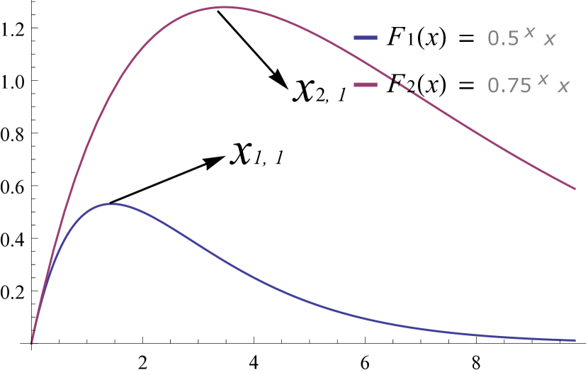
(a) Plot of $xp_{i}^{x}$ for $p_{1}=.5$, $p_{2}=.75$

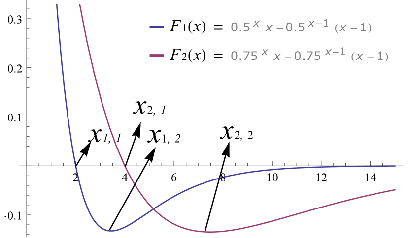
(b) Gradient of $xp_{i}^{x}$ for $p_{1}=.5$, $p_{2}=.75$

Figure 1: Characteristics of the IO-DOH Problem: For any $0<p_{i}<1$, there exist inflection points $x_{i,1}$ and $x_{i,2}$ for the function $F_{i}(x)=xp_{i}^{x}$ and its gradient, respectively. For the function $F_{i}(x)=xp_{i}^{x}$, the region from $x=0,\dots,x_{i,1}$ is convex, while the region beyond $x=x_{i,1}$ is not. Further, the inflection points ($x_{i,1}$ and $x_{i,2}$) and their corresponding values increase with an increase in $p_{i}$.

While a simple application of Jensens inequality [13] is sufficient to prove that the optimal allocation cannot be one where objects are split evenly, we are able to understand substantially more about the problem structure through the exchange arguments made to prove Lemmas 1 and 2 (resulting in Algorithms 5 and 3, respectively).

The Maximum Marginal Return algorithm [14] is a greedy approach which makes allocations of objects to the handlers that cause the greatest increase in the objective function. Lemma 1 shows that this technique always finds an optimal solution when $n\leq\sum_{i=1}^{k}x_{i,1}$. However, when $n>\sum_{i=1}^{k}x_{i,1}$, MMR is not optimal due to the absence of a convex structure as shown in Figure 1. In this case, Lemma 2 shows that an optimal solution has one sacrificial handler – i.e., it is beneficial to allow the highly probable destruction of one handler.

Lemma 1

The Maximum Marginal Return (MMR) algorithm returns an optimal solution when $n\leq\sum_{i=1}^{k}x_{i,1}$.

Proof

The following proof is via induction and an exchange argument that exploits the presence of the convex region of $F(x)$, as illustrated in Figure 1.

Clearly, MMR finds the optimal allocation when only one object is to be allocated. Since all objects are identical, we represent the allocation $S=\langle S_{1},\dots,S_{k}\rangle$ of $n$ objects to $k$ handlers by $O_{n,k}=\langle o_{1},\dots,o_{k}\rangle$, where $o_{i}=|S_{i}|$.

We assume that the solution returned by MMR for allocating $n$ objects to $k$ handlers – $O_{n,k}=\langle o_{1},\dots,o_{k}\rangle$ – is optimal. Let handler $i$ be the handler for which $F_{i}(o_{i}+1)-F_{i}(o_{i})$ is maximum – i.e., allocating a object to this handler causes the largest increase (or, smallest decrease) in the expected survival value. According to the MMR algorithm, the $n+1^{th}$ object is allocated to this handler – i.e., we have $OPT^{*}_{n+1,k}=\langle o^{*}_{1},\dots,o^{*}_{i},\dots,o^{*}_{k}\rangle=\langle o_{1},\dots,o_{i}+1,\dots,o_{k}\rangle$. The change in expected survival value for going from $OPT_{n,k}$ to $OPT^{*}_{n+1,k}$ is:

$$F^{\prime}_{i}(o_{i})=F_{i}(o_{i}+1)-F_{i}(o_{i})$$ (1)

Let $Z_{n+1,k}=\langle z_{1},\dots z_{k}\rangle$ be any other solution for allocating $n+1$ objects to $k$ handlers. Clearly, no optimal solution will have a handler $i$ with more than $x_{i,1}$ objects allocated to them (due to the fact that $x=x_{i,1}$ is a global maximum and strictly decreasing for all greater values of $x$) – therefore we will assume $z_{i}\leq x_{i,1}$ ($\forall i\in\{1,...,k\}$). Note that since $Z_{n+1,k}\neq OPT^{*}_{n+1,k}$, there must be some handler $j$ for which:

$$z_{j}>o^{*}_{j}\geq o_{j}$$ (2)

From this handler we remove a single object (in $Z_{n+1,k}$), to get an allocation given by $Z^{*}_{n,k}=\langle z^{*}_{1},\dots,z^{*}_{j},\dots,z^{*}_{k}\rangle=\langle z_{1},\dots,z_{j}-1,\dots,z_{k}\rangle$. The change in expected survival value for going from $Z^{*}_{n,k}$ to $Z_{n+1,k}$ is:

$$F^{\prime}_{j}(z^{*}_{j})=F_{j}(z_{j})-F_{j}(z_{j}-1)$$ (3)

Now, in $OPT_{n,k}$, we add a object to the same handler $j$ to get $\widehat{OPT}_{n+1,k}=\langle\widehat{o_{1}},\dots,\widehat{o_{j}},\dots,\widehat{o_{k}}\rangle=\langle o_{1},\dots,o_{j}+1,\dots,o_{k}\rangle$. The change in expected survival value for going from $OPT_{n,k}$ to $\widehat{OPT}_{n+1,k}$ is:

$$F^{\prime}_{j}(o_{j})=F_{j}(o_{j}+1)-F_{j}(o_{j})$$ (4)

Due to the assumption that $OPT_{n,k}$ is optimal, (2), and the fact that $x=x_{i,1}$ is an inflection point with strictly decreasing gradient until $x=x_{i,2}$ (see Figure 1), we have that (1) $\geq$ (4) $\geq$ (3). Therefore, the solution returned by MMR is at least as good as any other solution – i.e., $OPT^{*}_{n+1,k}\geq Z_{n+1,k}$.

Lemma 2

When $n>\sum_{i=1}^{k}x_{i,1}$, there is exactly one handler $i$ with more than $x_{i,1}$ objects allocated to it.

Proof

The following proof is via an exchange argument that exploits the structures of $F(x)$ and its gradient, as illustrated in Figure 1.

Since all objects are identical, we represent the allocation $S=\langle S_{1},\dots,S_{k}\rangle$ of objects to $k$ handlers by $O=\langle o_{1},\dots,o_{k}\rangle$, where $o_{i}=|S_{i}|$. Now, consider the allocation $O=\langle o_{1},\dots,o_{k}\rangle$. Let $o_{i}$ and $o_{j}$ be any two handlers with greater than $x_{i,1}$ and $x_{j,1}$ allocated objects, respectively. We have $ES_{i}+ES_{j}=F_{i}(x_{i,1}+\alpha)+F_{j}(x_{j,1}+\beta)$. Without loss of generality, we assume that $p_{i}\geq p_{j}$. Let $O^{*}$ be the allocation resulting from a move of $1$ object from handler $i$ to handler $j$. We have $ES^{*}_{i}+ES^{*}_{j}=F_{i}(x_{i,1}+\alpha-1)+F_{j}(x_{j,1}+\beta+1)$. The change in expected survival value is given by:

$$\left[F_{i}(x_{i,1}+\alpha-1)-F_{i}(x_{i,1}+\alpha)\right]+\left[F_{j}(x_{j,1}+\beta+1)-F_{j}(x_{j,1}+\beta)\right]$$

$$=F^{\prime}_{j}(x_{j,1}+\beta)-F^{\prime}_{i}(x_{i,1}+\alpha-1)$$ (5)

Let $\widehat{O}$ be the allocation resulting from a move of $1$ object from handler $j$ to handler $i$. We have $\widehat{ES}_{i}+\widehat{ES}_{j}=F_{i}(x_{i,1}+\alpha+1)+F_{j}(x_{j,1}+\beta-1)$. The change in expected survival value is given by:

$$\left[F_{i}(x_{i,1}+\alpha+1)-F_{i}(x_{i,1}+\alpha)\right]+\left[F_{j}(x_{j,1}+\beta-1)-F_{j}(x_{j,1}+\beta)\right]$$

$$=F^{\prime}_{i}(x_{i,1}+\alpha)-F^{\prime}_{j}(x_{j,1}+\beta-1)$$ (6)

Observe (in Figure 1) that $F_{i}^{\prime}(x)$ and $F^{\prime}_{j}(x)$ are strictly increasing functions for any input $x$ greater than $x_{i,2}$ and $x_{j,2}$, respectively, and there is some point $x\in\mathbf{R}^{+}$ where $F^{\prime}_{i}$ and $F^{\prime}_{j}$ intersect – i.e., $F^{\prime}_{j}(x-\epsilon)<F^{\prime}_{i}(x-\epsilon)$ and $F^{\prime}_{j}(x+\epsilon)>F^{\prime}_{i}(x+\epsilon)$. Therefore, for any $\beta$, there exists some $\gamma$ such that: $F^{\prime}_{j}(x_{j,1}+\beta)>F^{\prime}_{i}(x_{i,1}+\gamma)$ and $F^{\prime}_{j}(x_{j,1}+\beta)<F^{\prime}_{i}(x_{i,1}+\gamma-1)$.

• If $\alpha-1>\gamma$: (5) $>0$ – therefore, we can simply move $1$ object from handler $i$ to handler $j$ and obtain a better solution than $O$.

• If $\alpha-1\leq\gamma$: (6) $>0$ – therefore, we can simply move $1$ object from handler $j$ to $i$ and obtain a better solution than $O$.

Since we are able to make an improvement on any allocation containing two or more handlers with more than $x_{*,1}$ allocated objects, we have shown that no such solution may be optimal. Therefore, the optimal solution has exactly one handler $i$ with more than $x_{i,1}$ objects.

Corollary 1

When $n>\sum_{j=1}^{k}x_{j,1}$, if $|S_{i}|>x_{i,1}$ then $|S_{i}|=n-(\sum_{j\neq i}x_{j,1})$ and $|S_{j}|=x_{j,1}$, $\forall j\in\{1,\dots k\}\setminus\{i\}$.

Algorithm 3 The Identical Objects DOH Algorithm when $n>\sum_{i=1}^{k}x_{i,1}$

function IO-DOH($n,k,p_{1},\dots,p_{k},x_{1,1},\dots,x_{k,1}$)

     for $i=1\to k$ do

         $S_{i}\leftarrow\{\sum_{j=1}^{i-1}x_{j,1},\dots,\sum_{j=1}^{i}x_{j,1}\}$

     end for

     for $i=1\to k$ do

         $S_{i}\leftarrow S_{i}\bigcup\{\sum_{j=1}^{k}x_{j,1},\dots,n\}$

         if $\max<ES\langle S_{1},\dots,S_{k}\rangle$ then

              $\max\leftarrow ES\langle S_{1},\dots,S_{k}\rangle$ and $OPT\leftarrow\langle S_{1},\dots,S_{k}\rangle$

         end if

     end for

     return $OPT$

end function

In the case where $n\leq\sum_{i=1}^{k}x_{i,1}$, algorithm 3 runs the MMR algorithm to find an allocation. By lemma 1, this is optimal.

In the case where $n>\sum_{i=1}^{k}x_{i,1}$, algorithm 3 goes through $k$ iterations. In the $i^{th}$ iteration, it allocates $x_{j,1}$ objects to the $j^{th}$ handler ($\forall j\in\{1,\dots,k\}\setminus\{i\})$ and the remaining objects to the $i^{th}$ handler. Following this, the $ES$ of the allocation is computed and stored in the $i^{th}$ index of an array. The algorithm returns the allocation corresponding to the maximum value in this array as the optimal allocation. By lemma 2 and corollary 1, this is the optimal allocation.

4.2 Identical Handlers and Values

In this case, we require that each object has the same value and possesses failure probabilities that are object dependent (but, handler independent) – i.e., w.l.o.g., we have $v_{j}=1$ and $p_{ij}=p_{j}$ ($\forall i\in\{1,\dots,k\}$ and $\forall j\in\{1,\dots,n\}$). Now the problem can be stated as:

Problem 3

The Identical Handlers and Values DOH (IHV-DOH) problem: Given $p_{ij}=p_{j}$ and $v_{j}=1$ for $i=1,\dots k$ and $j=1\dots,n$, find partition $S_{1}\cup\dots\cup S_{k}$ of $\{1,\dots,n\}$ that maximizes $ES=\sum_{i=1}^{k}ES_{i}$, where $ES_{i}=|S_{i}|\prod_{j\in S_{i}}p_{j}$.

Observe that if instead, not all objects had identical values, the problem would be $\mathsf{NP}$-$\mathsf{complete}$ as shown in theorem 2.1.

Theorem 4.1

Assuming that objects are ordered by decreasing survival probabilities ($p_{j}$), each handler receives a contiguous subsequence of objects.

Proof

Without loss of generality, let $p_{1}\geq p_{2}\geq\dots\geq p_{n}$. Consider the allocation given by $S=\langle S_{1},\dots,S_{k}\rangle$ where $\forall i\in\{1,\dots,k-1\}$: $ES_{i}\geq ES_{{i+1}}$. Let $S_{i}$ be the first handler with a non-contiguous allocation – i.e., object $l\in S_{i}$ but object $m\in S_{i+1}$ (where $p_{l}\leq p_{m}$). Now, consider the allocation given by $S^{*}=\langle S_{1},\dots,S^{*}_{i},S^{*}_{i+1},\dots,S_{k}\rangle$ where object $l\in S^{*}_{i+1}$ and object $m\in S^{*}_{i}$ – i.e., the allocation where the handlers of object $l$ and $m$ are swapped. Now, observe that: $\left[ES_{i}+ES_{{i+1}}\right]-\left[ES^{*}_{i}+ES^{*}_{{i+1}}\right]$=$\left[ES_{i}+ES_{{i+1}}\right]-\left[\frac{p_{m}}{p_{l}}ES_{i}+\frac{p_{l}}{p_{m}}ES_{{i+1}}\right]$
$\leq\left[ES_{i}+ES_{{i+1}}\right]-\left[ES_{i}+ES_{{i+1}}\left(\frac{p_{l}}{p_{m}}+\frac{p_{m}}{p_{l}}-1\right)\right]\leq 0$. Therefore, the expected survival value of a contiguous allocation is always at-least as good as any non-contiguous allocation.

Since the optimal allocation of objects to handlers is contiguous (given objects sorted by their survival probabilities), the following recursive relation may be used to find the optimal allocation.

$$OPT(i,j)=\max_{1\leq l\leq i}\left[\left(i-l\right)\prod_{m=l}^{i}p_{m}+OPT(l,j-1)\right]$$

where $OPT(i,0)=\infty$ and $OPT(n,k)$ returns the maximum expected survival value for $n$ objects allocated to $k$ handlers in $O(n^{2}k)$ time.

4.3 Identical Risks

In this case, we require that each object possesses a distinct value and failure probabilities that are handler dependent (but, object independent) – i.e., w.l.o.g., we have $p_{ij}=p_{i}$ ($\forall i\in\{1,\dots,k\}$ and $\forall j\in\{1,\dots,n\}$). Now the problem can be stated as the following:

Problem 4

The Identical Risk DOH (IR-DOH) problem: Given $p_{ij}=p_{i}$ and for $i=1,\dots k$ and $j=1\dots,n$, find partition $S_{1}\cup\dots\cup S_{k}$ of $\{1,\dots,n\}$ that maximizes $ES=\sum_{i=1}^{k}ES_{i}$, where $ES_{i}=\sum_{j\in S_{i}}v_{j}p_{i}^{|S_{i}|}$.

Theorem 4.2

Assuming that objects are ordered by decreasing values ($v_{j}$) and handlers are ordered by decreasing survival probabilities($p_{i}$), each handler receives a contiguous subsequence of objects.

Proof

Let $v_{1}\geq v_{2}\geq\dots\geq v_{n}$. Consider the allocation given by $S=\langle S_{1},\dots,S_{k}\rangle$ where without loss of generality, $p_{1}^{|S_{1}|}\geq p_{2}^{|S_{2}|}\geq\dots\geq p_{k}^{|S_{k}|}$. Let $S_{i}$ be the first handler with a non-contiguous allocation – i.e., object $l\in S_{i}$ but object $m\in S_{i+1}$ (where $v_{l}\leq v_{m}$). Now, consider the allocation given by $S^{*}=\langle S_{1},\dots,S^{*}_{i},S^{*}_{i+1},\dots,S_{k}\rangle$ where object $l\in S^{*}_{i+1}$ and object $m\in S^{*}_{i}$ – i.e., the allocation where the handlers of object $l$ and $m$ are swapped. Now, observe that:

$$\left[ES_{i}+ES_{{i+1}}\right]-\left[ES^{*}_{i}+ES^{*}_{{i+1}}\right]=$$

$$\left[p_{i}^{|S_{i}|}V_{i}+p_{i+1}^{|S_{i+1}|}V_{{i+1}}\right]-\left[p_{i}^{|S_{i}|}(V_{i}+v_{m}-v_{l})+p_{i+1}^{|S_{i+1}|}(V_{{i+1}}+v_{l}-v_{m})\right]=$$

$$\left[p_{i}^{|S_{i}|}(v_{m}-v_{l})-p_{i+1}^{|S_{i+1}|}(v_{l}-v_{m})\right]\leq 0.$$

Therefore, the expected survival value of a contiguous allocation is always at-least as good as any non-contiguous allocation.

Since the optimal allocation of objects to handlers is contiguous (given objects sorted by their values), the following recursive relation may be used to find the optimal allocation.

$$OPT(i,j)=\max_{1\leq l\leq i}\left[p_{j}^{i-l}\sum_{m=l}^{i}v_{m}+OPT(l,j-1)\right]$$ (7)

where $OPT(i,0)=\infty$ and $OPT(n,k)$ returns the maximum expected survival value for $n$ objects allocated to $k$ handlers in $O(n^{2}k)$ time.

4.4 Identical Risks, Values and Handlers

Under the assumption that all objects and handlers are identical, w.l.o.g., we have $v_{j}=1$ and $p_{ij}=p$ ($\forall i\in\{1,\dots,k\}$ and $\forall j\in\{1,\dots,n\}$). In this case, the generic DOH problem may be re-stated as:

Problem 5

The Identical Objects and Identical Handlers DOH (IOIH-DOH) problem: Given $p_{ij}=p$ and $v_{j}=1$ for $i=1,\dots k$ and $j=1\dots,n$, find partition $S_{1}\cup\dots\cup S_{k}$ of $\{1,\dots,n\}$ that maximizes $ES=\sum_{i=1}^{k}ES_{i}$, where $ES_{i}=|S_{i}|p^{|S_{i}|}$.

We make the following observations about $F(x)=xp^{x}$, where $x\in\mathbf{Z}^{+}$:

• For any $p$ such that $0<p<1$, there exists an $x_{1}$ such that $F(x_{1})\geq F(x_{1}+\alpha)$ and $F(x_{1})\geq F(x_{1}-\alpha)$, where $\alpha\in\mathbf{Z}^{+}$ and there exists an $x_{2}$ such that $F^{\prime}(x_{2})\leq F^{\prime}(x_{2}+\beta)$ and $F^{\prime}(x_{2})\leq F^{\prime}(x_{2}-\beta)$, where $\beta\in\mathbf{Z}^{+}$.

• $\forall x\in\{0,\dots,x_{1}-1\}$: $F(x)>0$, $F^{\prime}(x)>0$, and $F^{\prime\prime}(x)<0$.

• $\forall x\in\{x_{1}+1,\dots,\infty\}$: $F(x)>0$ and $F^{\prime}(x)\leq 0$.

• $\forall x\in\{x_{1}+1,\dots,x_{2}\}$: $F^{\prime\prime}(x)\leq 0$ and $\forall x\in\{x_{2}+1,\dots,\infty\}$: $F^{\prime\prime}(x)\geq 0$.

Algorithm 4 IOIH-DOH Solver

if $x_{1}>n$ then

     $x_{1}\leftarrow n$.

end if

if $n\leq kx_{1}$ then

     $OPT\leftarrow\langle\lfloor\frac{n}{k}\rfloor,\dots,\lfloor\frac{n}{k}\rfloor,\lceil\frac{n}{k}\rceil,\dots,\lceil\frac{n}{k}\rceil\rangle$ such that $\sum_{i=1}^{k}OPT_{i}=n$.

end if

if $n>kx_{1}$ then

     $O\leftarrow\langle x_{1},\dots,x_{1},n-(k-1)x_{1}\rangle$

     for $i=1\to k-1$ do

         if $\left[F(O_{k}-1)-F(O_{k})\right]>\left[F(O_{i})-F(O_{i}+1)\right]$ then

              $O_{k}\leftarrow O_{k}-1$

              $O_{i}\leftarrow O_{i}+1$

         end if

     end for

     $OPT\leftarrow O$

end if

return $OPT$

Lemma 3

In any optimal allocation for problem 5 with $n\leq kx_{1}$, the objects are split amongst handlers as evenly as possible.

Proof

Consider the allocation $O=\langle o_{1},\dots,o_{k}\rangle$ with $|o_{i}|>x_{1}$ and $|o_{j}|<x_{1}$. We have $ES_{i}+ES_{j}=F(x_{1}+\alpha)+F(x_{1}-\beta)$. By moving a single object from $o_{i}$ to $o_{j}$, we get the allocation $O^{*}$ where $ES^{*}_{i}+ES^{*}_{j}=F(x_{1}+\alpha-1)+F(x_{1}+\beta+1)$. By O2 and O3, $[ES^{*}_{i}-ES_{i}]+[ES^{*}_{j}-ES_{j}]>0$. Therefore, $O^{*}$ is strictly better than $O$.

Lemma 4

In any optimal allocation for problem 5 with $n>kx_{1}$, exactly $1$ handler is allocated more than $x_{1}+1$ objects.

Proof

Consider the allocation $O=\langle o_{1},\dots,o_{k}\rangle$ with $|o_{i}|\geq|o_{j}|>x_{1}+1$. We have $ES_{i}+ES_{j}=F(x_{1}+\alpha)+F(x_{1}+1+\beta)$. If $F(x_{1})-F(x_{1}+1)<F(x_{1}+\alpha+\beta)-F(x_{1}+\alpha+\beta+1)$, then we move $\beta$ objects from $o_{j}$ to $o_{i}$ to get the allocation $O^{*}$ where $ES^{*}_{i}+ES^{*}_{j}=F(x_{1}+\alpha+\beta)+F(x_{1}+1)$. Otherwise, we move $\beta+1$ objects from $o_{j}$ to $o_{i}$ to get the allocation $\widehat{O}$ where $\widehat{ES}_{i}+\widehat{ES}_{j}=F(x_{1}+\alpha+\beta+1)+F(x_{1})$. By O3 and O4, we have either $[ES^{*}_{i}-ES_{i}]+[ES^{*}_{j}-ES_{j}]>0$ or $[\widehat{ES}_{i}-ES_{i}]+[\widehat{ES}_{j}-ES_{j}]>0$. Therefore, $O$ can never be optimal.

Note: If $x_{1}\in\mathbf{R}^{+}$ (rather than $x_{1}\in\mathbf{Z}^{+}$), it is always true that $F(x_{1})-F(x_{1}+1)>F(x_{1}+\alpha+\beta)-F(x_{1}+\alpha+\beta+1)$. Therefore, the optimal allocation would always have exactly $k-1$ handlers with exactly $x_{1}$ objects allocated to each of them.

Theorem 4.3

Algorithm 4 always finds an optimal allocation for problem 5.

Proof

In the case where $n\leq kx_{1}$, algorithm 4 returns the allocation where objects are split as evenly as possible amongst the handlers. By lemma 3, this is optimal.

In the case where $n>kx_{1}$, algorithm 4 first allocates exactly $x_{1}$ objects to each of $k-1$ handlers and the remaining objects to the $k^{th}$ handler. Then, if we have $F(x_{1})-F(x_{1}+1)<F(O_{k}-1)-F(O_{k})$, we move one object from the $k^{th}$ handler to one of the other $k-1$. This shifting process is repeated until the condition is no longer true (at-most $k-1$ iterations). By lemma 4, this is optimal.

4.5 Exactly One Object per Handler

In this section we consider the original formulation defined in problem 1, this time with the restriction that handlers may be allocated only exactly one object. We will show that under this assumption, the problem can be stated as an instance of the transportation problem (a special case of the min cost - max flow problem with a linear objective function) [15]. This special case can be stated as the following:

Problem 6

The Exactly One DOH (EO-DOH) problem: Given $v_{1},\dots,v_{n}$ and $p_{ij}$ for $i=1,\dots k$ and $j=1\dots,n$, find partition $S_{1}\cup\dots\cup S_{k}$ of $\{1,\dots,n\}$ that maximizes $ES=\sum_{i=1}^{k}ES_{i}$, where $ES_{i}=\sum_{j\in S_{i}}v_{j}\prod_{j\in S_{i}}p_{ij}$ and $|S_{i}|=1$ for $i=1,\dots,k$.

Since $|S_{i}|=1$, the following identities are observed: (1) $\prod_{j\in S_{i}}p_{ij}=\sum_{j\in S_{i}}p_{ij}$ and (2) $(\sum_{j\in S_{i}}p_{ij})(\sum_{j\in S_{i}}v_{j})=\sum_{j\in S_{i}}p_{ij}v_{j}$. These identities allow us to convert problem 6 into the instance of an (unbalanced) transportation problem [16], [17] defined in problem 7.

Problem 7

The Unbalanced Transportation Problem: Given $v_{1},\dots,v_{n}$ and $p_{ij}$ for $i=1,\dots k$ and $j=1\dots,n$, find partition $S_{1}\cup\dots\cup S_{k}$ of $\{1,\dots,n\}$ that maximizes $ES=\sum_{i=1}^{k}ES_{i}$, where $ES_{i}=\sum_{j\in S_{i}}v_{j}p_{ij}$.

Problem 7 is a well studied problem with efficient methods for obtaining solutions based on successive shortest-path generalizations [18], minimum mean cycle cancelling [19], and poly-time network simplex methods[20].

5 Heuristics

In this section we propose and evaluate five heuristics for finding solutions to DOH problems. The heuristics are based on the MMR algorithm (Algorithm 5), dynamic programming approach (Section 3), and genetic algoritms. A performance comparison of the heuristics is provided in Table 2.

Ordered MMR for DOH Problems (O-MMR):

In this heuristic, objects are ordered by decreasing values before the standard MMR greedy approach (Section 4) is used as usual. Experimental analysis reveals that in most cases, such an ordering (usually) performs better than MMR where objects are either unordered, or ordered by increasing values.

Clairvoyant MMR for DOH Problems (C-MMR):

The following variation is made to the O-MMR algorithm: If there is no handler to which the current object can be allocated without causing a drop in the cumulative expected survival value, then that object is placed in a dumpster handler. After initial allocation of all objects is complete, all objects in the dumpster are allocated together (as a single object) to the one handler that experiences the smallest loss in ES value.

Algorithm 5 The MMR, OMMR, and CMMR Algorithms

function MMR($n,k,v_{1},\dots,v_{n},p_{11},\dots,p_{kn},type$)$\triangleright$ $type\leftarrow 1$ for OMMR, $2$ for CMMR, $0$ otherwise

    for $i=1\to k$ do

         $S_{i}\leftarrow\emptyset$, $ES_{i}\leftarrow 0$, $S_{dumpster}\leftarrow\emptyset$

    end for

    if $type\geq 1$ then

         $\textsc{sort}(v_{1},\dots,v_{n},p_{11},\dots,p{kn})$$\triangleright$ sort values and re-arrange probabilities accordingly

    end if

    for $i=1\to n$ do

         for $j=1\to k$ do

             $T_{j}\leftarrow S_{j}\bigcup i$, $\delta_{j}\leftarrow\textsc{Compute-ES}(T_{j})-ES_{j}$

         end for

         $m\leftarrow\arg\max\{\delta_{1},\dots,\delta_{k}\}$

         if $cmmr=1\land\delta_{m}<0$ then

             $S_{dumpster}\leftarrow S_{dumpster}\bigcup i$

         else

             $S_{m}\leftarrow S_{m}\bigcup i$, $ES_{m}\leftarrow\textsc{Compute-ES}(S_{m})$

         end if

    end for

    if $type=2$ then

         for $j=1\to k$ do

             $T_{j}\leftarrow S_{j}\bigcup S_{dumpster}$, $\delta_{j}\leftarrow\textsc{Compute-ES}(T_{j})-ES_{j}$

         end for

         $m\leftarrow\arg\max\{\delta_{1},\dots,\delta_{k}\}$

    end if

    return $\langle S_{1},\dots,S_{k}\rangle$

end function

Dynamic Programming Based Heuristic (DP-H):

The DP-H algorithm is a variation of the FPTAS presented in Section 3. The major difference is that the DP-H algorithm maintains exactly $n$ states for each iteration of the dynamic program. In each iteration, the $n$ most promising states are maintained while the remaining are culled. To do this, we divide the state space into $n$ uniformly sized blocks and maintain at-most $n$ states for each iteration of the dynamic program – i.e., the state with the highest ES for each block. Therefore, in each iteration, no more than $n$ promising states are maintained while the remaining are culled. Finally, after all $n$ accounts are allocated, the state with the maximum ES is returned. The algorithm is illustrated in algorithm 6.

Algorithm 6 DP-H trimming procedure

function Trim($\Phi$) $\triangleright$ Trim function for computing DP-H solutions

     for all $(V_{1},\dots,V_{k},P_{1},\dots,P_{k})\in\Phi$ do

         Find $\langle{r_{1}},\dots,{r_{k}}\rangle$ such that $\frac{(r_{i}+1)V_{max}}{n^{1/k}}\leq V_{i}\leq\frac{r_{i}V_{max}}{n^{1/k}}$, $\forall i\in\{1,\dots,k\}$

         Find $\langle s_{1},\dots,{s_{k}}\rangle$ such that $\frac{(s_{i}+1)P_{max}}{n^{1/k}}\leq P_{i}\leq\frac{s_{i}P_{max}}{n^{1/k}}$, $\forall i\in\{1,\dots,k\}$

         $CurrES\leftarrow\textsc{Compute-ES}(V_{1},\dots,V_{k},P_{1},\dots,P_{k})$

         if $Orthotope[\langle r_{1},\dots,r_{k},s_{1},\dots,s_{k}\rangle]=\perp$ then

              $Orthotope[\langle r_{1},\dots,r_{k},s_{1},\dots,s_{k}\rangle]\leftarrow(V_{1},\dots,V_{k},P_{1},\dots,P_{k})$

              $ESofOrthotope[\langle r_{1},\dots,r_{k},s_{1},\dots,s_{k}\rangle]\leftarrow CurrES$

         end if

         if $ESofOrthotope[\langle r_{1},\dots,r_{k},s_{1},\dots,s_{k}\rangle]<CurrES$ then

              $Orthotope[\langle r_{1},\dots,r_{k},s_{1},\dots,s_{k}\rangle]\leftarrow(V_{1},\dots,V_{k},P_{1},\dots,P_{k})$

              $ESofOrthotope[\langle r_{1},\dots,r_{k},s_{1},\dots,s_{k}\rangle]\leftarrow CurrES$

         end if

     end for

     return $Orthotope$

end function

Random Initialization with Complete Genetic Inheritance (RI-GA):

We refer to each DOH candidate solution as an individual and each single object-to-handler assignment as a chromosome of that individual. The fitness function used to evaluate an individual is simply function that computes its corresponding ES value. In each iteration, the fitness of all individuals is evaluated and a fixed number of couples are selected based on the standard roulette wheel selection [21]. After the mutation procedure, each couple is replaced with their offspring.

In the RI-GA algorithm, the initial population is randomly generated. The child $(c)$ of each couple $(p_{1},p_{2})$ is created by inheriting every chromosome from one of $p_{1}$ or $p_{2}$. The most profitable non-overlapping handlers (set of chromosomes) of $p_{1}$ and $p_{2}$ are inherited in decreasing order. Finally, if no more chromosome sets may be completely inherited and the child is still incomplete, the child inherits each of its remaining chromosomes from parent $p_{i}$ with probability $\frac{fitness(p_{i})}{(fitness(p_{1})+fitness(p_{2}))}$.

Heuristic Based Initialization with Partial Genetic Inheritance (HI-GA):

In the HI-GA algorithm, the initial population is seeded as follows: $60\%$ are randomly generated, $15\%$ are populated by the allocation generated by O-MMR, $15\%$ are populated by the allocation generated by C-MMR, and the final $10\%$ are populated by the allocation generated by DP-H. The mutation procedure is similar to RI-GA, except if no more chromosome sets may be completely inherited and the child is still incomplete, the child spawns randomly generated chromosomes (which may completely differ from either parent).

In the evaluation of the RI-GA and HI-GA algorithms, the initial population was set to be 1000. Further, in each generation, 1000 pairs of individuals were chosen to produce 1000 children (the population was always exactly 1000). The fittest child after 1000 generations was returned as the solution.

n	k	O-MMR		C-MMR		DP-H		RI-GA		HI-GA
		$\mu$	$\sigma$	$\mu$	$\sigma$	$\mu$	$\sigma$	$\mu$	$\sigma$	$\mu$	$\sigma$
25	5	.398	.070	.380	.066	.398	.069	.448	.061	.464	.056
	10	.759	.044	.767	.050	.759	.045	.705	.048	.767	.044
50	10	.585	.047	.561	.046	.585	.046	.459	.047	.588	.044
	25	.908	.013	.910	.013	.908	.015	.685	.038	.910	.036
100	25	.832	.019	.829	.024	.831	.020	.445	.043	.831	.019
	50	.950	.006	.950	.006	.941	.006	.559	.030	.950	.006
250	25	.654	.021	.639	.022	.654	.021	.121	.029	.681	.028
	50	.890	.008	.886	.009	.889	.008	.221	.027	.891	.008
	100	.969	.002	.970	.002	.969	.002	.348	.022	.970	.022

Table 2: Mean ($\mu$) and Standard Deviation ($\sigma$) of the ratio between the ES obtained by the heuristic and the upper-bound ES value for varying $n$ and $k$ (50 trials per experiment).

6 Conclusions and Future Work

The Destructive Object Handler problem describes many real-world situations in which dangerous objects must be shipped, processed, quarantined, or otherwise handled, and the destruction of one object assigned to a handler destroys all the other objects assigned to the same handler. We have shown that this problem is NP-complete in general, but have provided an FPTAS when the number of handlers is constant and polynomial time algorithms for numerous special cases. We have evaluated several heuristics based on simple greedy strategies, dynamic programming, and genetic algorithms. It appears that the heuristics perform poorly when the ratio of objects to handlers is high, but improve as this ratio reduces (even for very large problem sizes).

There remain many open avenues for research on the DOH problem, particularly in understanding its complexity. The hardness of the generic DOH problem is still not fully known – i.e., it remains unknown if the DOH problem is solvable by a pseudo-polynomial time algorithm or if there exists a reduction that proves its strong $\mathsf{NP}$-$\mathsf{Completeness}$. We also have not studied the special case when all objects have identical values. Further, it is not known if efficient constant factor or $(1-\epsilon)$ approximations exist when $k$ is not a constant.

References

• [1] Manne, A.S.: A target-assignment problem. Operations Research 6(3) (1958) pp. 346–351
• [2] Florencio, D., Herley, C.: A large-scale study of web password habits. In: Proceedings of the 16th international conference on World Wide Web. WWW ’07 (2007)
• [3] Perlroth, N.: Lax Security at LinkedIn Is Laid Bare. The New York Times (June 11, 2012)
• [4] Perito, D., Castelluccia, C., Kaafar, M., Manils, P.: How unique and traceable are usernames? In: Privacy Enhancing Technologies. (2011) 1–17
• [5] Finkle, J.: Yahoo breach puts users of other sites at risk. Reuters (July 13, 2012)
• [6] Lloyd, S., Witsenhausen, H.: Weapon-Target Allocation is NP Complete. Proceedings of the Summer Computer Simulation Conference (1986) 1054–1059
• [7] Erkut, E., Verter, V.: Modeling of transport risk for hazardous materials. Operations Research 46(5) (1998) pp. 625–642
• [8] Berman, O., Verter, V., Kara, B.: Designing Emergency Response Networks for Hazardous Materials Transportation. Centre for Research on Transportation (2004)
• [9] Erkut, E., Gzara, F.: Solving the hazmat transport network design problem. Comput. Oper. Res. 35(7) (July 2008) 2234–2247
• [10] Tarantilis, C., Kiranoudis, C.: Using the vehicle routing problem for the transportation of hazardous materials. Operational Research 1(1) (2001) 67–78
• [11] Garey, M., Johnson, D.: Complexity results for multiprocessor scheduling under resource constraints. SIAM Journal on Computing 4(4) (1975) 397–411
• [12] Woeginger, G.J.: When does a dynamic programming formulation guarantee the existence of an fptas? In: Proceedings of the tenth annual ACM-SIAM symposium on Discrete algorithms. SODA ’99 (1999) 820–829
• [13] Hardy, G., Littlewood, J., Pólya, G.: Inequalities. Cambridge Mathematical Library. Cambridge University Press (1952)
• [14] Kolitz, S.: Analysis of a maximum marginal return assignment algorithm. In: Decision and Control, 1988., Proceedings of the 27th IEEE Conference on. (1988)
• [15] Schrijver, A.: Combinatorial Optimization: Polyhedra and Efficiency. Number v. 1 in Algorithms and Combinatorics. Springer (2003)
• [16] Kantorovitch, L.: On the translocation of masses. Management Science 5(1) (1958) 1–4
• [17] Munkres, J.: Algorithms for the assignment and transportation problems. Journal of the Society for Industrial & Applied Mathematics 5(1) (1957) 32–38
• [18] Goldberg, A.V., Tarjan, R.E.: Finding minimum-cost circulations by successive approximation. Math. Oper. Res. 15(3) (July 1990) 430–466
• [19] Goldberg, A.V., Tarjan, R.E.: Finding minimum-cost circulations by canceling negative cycles. J. ACM 36(4) (October 1989) 873–886
• [20] Orlin, J.B.: A polynomial time primal network simplex algorithm for minimum cost flows. In: Proceedings of the seventh annual ACM-SIAM symposium on Discrete algorithms. SODA ’96 (1996) 474–481
• [21] Bäck, T.: Evolutionary algorithms in theory and practice: evolution strategies, evolutionary programming, genetic algorithms. Oxford University Press (1996)