The oscillating behavior of the pair correlation function in galaxies

Abstract

The pair correlation function (PCF) for galaxies presents typical oscillations in the range 20-200 Mpc/h which are named baryon acoustic oscillation (BAO). We first review and test the oscillations of the PCF when the 2D/3D vertexes of the Poissonian Voronoi Tessellation (PVT) are considered. We then model the behavior of the PCF at a small scale in the presence of an auto gravitating medium having a line/plane of symmetry in 2D/3D. The analysis of the PCF in an astrophysical context was split into two, adopting a non-Poissonian Voronoi Tessellation (NPVT). We first analyzed the case of a 2D cut which covers few voids and a 2D cut which covers approximately 50 voids. The obtained PCF in the case of many voids was then discussed in comparison to the bootstrap predictions for a PVT process and the observed PCF for an astronomical catalog. An approximated formula which connects the averaged radius of the cosmic voids to the first minimum of the PCF is given.

Dipartimento di Fisica , Via Pietro Giuria 1, 10125, Turin, Italy

Keywords: methods: statistical; cosmology: observations; (cosmology): large-scale structure of the Universe

1 Introduction

The computation of pair correlation functions (PCF) started with the experimental evaluation of the PCF of liquid argon from neutron scattering, see Yarnell et al. (1973). The PCF was then treated in many books as a subject connected to mono-atomic fluids, see McQuarrie (1976); Hansen, J. P. and McDonald, I. R. (1986); Allen and Tildesley (1987). The PCF was later applied to the Poissonian Voronoi Tessellation (PVT) and the PCF for 2D/3D vertexes was evaluated, see Stoyan and Stoyan (1990); Okabe et al. (2000); Heinrich and Muche (2008). The astronomers started to study the baryon acoustic oscillations (BAO) as a tool for probing the cosmological distance scale and dark energy, see Eisenstein et al. (2005). The astronomical analysis continued with the study of: (i) the impact of uncertainties in the photometric redshift error probability distribution on dark energy constraints from the detection of BAO in galaxy power spectra, see Zhan and Knox (2006), (ii) the cosmological distance errors achievable using the BAO as a standard ruler, see Seo and Eisenstein (2007), (iii) the detectability of BAO in the power spectrum of galaxies using ultra large volume $N$-body simulations of the hierarchical clustering of dark matter and semi-analytical modeling of galaxy formation, see Angulo et al. (2008), (iv) a set of ultra-large particle-mesh simulations of the Lyman-$\alpha$ forest targeted at understanding the imprint of BAO in the inter-galactic medium, see White et al. (2010), (v) the use of BAO to map the expansion history of the universe, see Mehta et al. (2011), (vi) a measure of BAO from the angular power spectra of the Sloan Digital Sky Survey III (SDSS-III) Data Release 8 imaging catalog that includes 872,921 galaxies over 10000 ${{\mathrm{deg}}}^{2}$ between 0.45 $<z<0.65$, see Seo et al. (2012).

2 The PCF

This Section outlines the difference between PCF in fluids and PCF in astronomy. The PCF adopted for Voronoi Diagrams is reviewed.

2.1 The PCF in fluids

The PCF gives the probability of finding a pair of objects a distance $r$ apart, relative to the probability expected for a random distribution of the same density. This function can be estimated as

$$g(r)=\frac{V}{N^{2}}\langle\Sigma_{j}\Sigma_{j\neq i}\delta({\bf r}-{\bf r}_{ij})\rangle\quad,$$ (1)

where $V$ is the considered volume, $N$ is the number of objects, and ${\bf r}_{ij}$ is the distance between centers, see formula (2.94) in Allen and Tildesley (1987).

2.2 The PCF in astronomy

Astronomers, beginning with Totsuji and Kihara (1969) , have used the following convention for the PCF for galaxies

$$\xi_{{\mathrm{GG}}}(r)=1+g(r)\quad.$$ (2)

The most used conventions for low values of $r$ assumes that

$$\xi_{{\mathrm{GG}}}=({r\over r_{{\mathrm{G}}}})^{-\gamma_{{\mathrm{GG}}}}\quad,$$ (3)

where $\gamma_{{\mathrm{GG}}}$=1.8 and $r_{{\mathrm{G}}}=5.77h^{-1}{{\mathrm{Mpc}}}$ (the correlation length) when the range $0.1h^{-1}{{\mathrm{Mpc}}}<r<16h^{-1}{{\mathrm{Mpc}}}$ is considered, see Zehavi et al. (2004) where 118,149 galaxies were analyzed. Another estimator of the PCF useful both for simulations of vertexes of PVT and catalogs of galaxies is

$$\xi_{{\mathrm{OO}}}=1+\frac{n_{{\mathrm{OO}}}(r)}{n_{{\mathrm{RR}}}(r)}-2\frac{n_{{\mathrm{OR}}}(r)}{n_{{\mathrm{RR}}}(r)}\quad.$$ (4)

where $n_{{\mathrm{OO}}}(r)$, $n_{{\mathrm{RR}}}(r)$, and $n_{{\mathrm{OR}}}(r)$ are the number of object–object, random–random, and object–random pairs having distance $r$, see Szalay et al. (1993); Martínez et al. (2009); in this paper the word object can be substituted by a vertex of a PVT or a galaxy. The random configuration can be realized every time with a different random number generator. As an example, we generate $N_{{\mathrm{T}}}$ different random configurations and we average the different values of $\xi_{{\mathrm{OO}}}$ which now will be characterized by an error bar given by the standard deviation.

2.3 The PCF in Voronoi Diagrams

The PCF for the point process of vertexes in ${\bf R}^{2}$ and ${\bf R}^{3}$ has been analyzed by Stoyan and Stoyan (1990); Okabe et al. (2000); Heinrich and Muche (2008). A review formula for the PCF is reported in Okabe et al. (2000), see Eqn. (5.6.2) with m=2 (2D) and m=3 (3D) and Tables 5.6.1 and 5.6.2; as a first analysis we tested the 2D and 3D results with our simulation. In this case the PCF is computed via the numerical formula (4). The adopted scale is important and in view of future applications we have chosen the generalized averaged radius, $\bar{R}$, of the 2D cells as

$$\pi{\bar{R}}^{2}=\frac{L^{2}}{N}\quad,$$ (5)

where $L$ is the side of the square in which $N_{{\mathrm{s}}}$ seeds are inserted. The generalized averaged radius in 3D is

$$\frac{4}{3}\pi{\bar{R}}^{3}=\frac{L^{3}}{N}\quad,$$ (6)

where $L$ is the side of the cube in which $N_{{\mathrm{s}}}$ seeds are inserted. The distances will therefore be expressed in normalized units $r/\bar{R}$ and as an example a normalized distance of 2 corresponds to an averaged diameter. Figures (1) and (2) report the 2D/3D mathematical PCF as well our simulated one in normalized units.

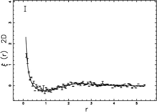
Figure 1: The values of the PCF for the point process of vertexes of 2D PVT, in ${\bf R}^{2}$ (full line) as extracted from Table 5.6.1 in Okabe et al. (2000). The simulated PCF as given by Eq. (4) is reported as the dashed line with error bar. The distances are expressed in normalized units, the number $N_{{\mathrm{s}}}$ of seeds is 1000, and $N_{{\mathrm{T}}}$=10.

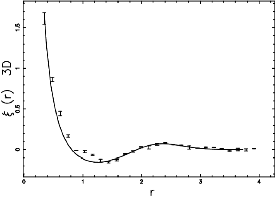
Figure 2: Values of the PCF for the point process of vertexes of 3D PVT, in ${\bf R}^{3}$ (full line) as extracted from Table 5.6.2 in Okabe et al. (2000). The simulated PCF as given by Eq. (4) is reported as a dashed line with error bar. The distances are expressed in normalized units, the number, $N_{{\mathrm{s}}}$, of seeds is 800 and $N_{{\mathrm{T}}}$= 5.

We are in the presence of a damped oscillatory behavior of the PCF for PVT vertexes and the first minimum is reached when $r/\bar{R}\approx 1$ in 2D and $r/\bar{R}\approx 1.4$ in 3D.

3 Galaxies on the faces

This section first reviews the statistical distributions as function of the height from a plane of reference for a system of auto gravitating galaxies and then provides a first astrophysical environment when we have a symmetrical configuration of galaxies in respect to a line (2D) or in respect to a plane (3D).

3.1 Self-gravitating galaxies

The density profile of a thin self-gravitating disk of gas which is characterized by a Maxwellian distribution in velocity and a distribution which varies only in the $z$-direction is here applied to galaxies,

$$n(z;z_{0})=n_{0}sech^{2}(\frac{z}{2\,z_{0}})\quad,$$ (7)

where $n_{0}$ is the galaxy density at $z=0$, $z_{0}$ is a scaling parameter in ${{\mathrm{Mpc}}}/h$, and $sech$ is the hyperbolic secant (Spitzer (1942); Rohlfs (1977); Bertin (2000); Padmanabhan (2002)). This physical law can be converted to a probability density function (PDF), the probability of having a galaxy at a distance between $z$ and $z+dz$ from a plane of symmetry

$$p(z;z_{0})=\frac{1}{4}\,\left({\it sech}\left(\frac{1}{2}\,{\frac{\left|z\right|}{z_{{0}}}}\right)\right)^{2}\frac{1}{z_{0}}\quad.$$ (8)

The range of existence of this PDF, which is the logistic distribution, is in the interval $[-\infty,\infty]$, see Balakrishnan (1991); Johnson et al. (1995); Evans et al. (2000). The average value is $E(z;z_{0})=0$ and the variance is

$$\sigma^{2}(z;z_{0})=\frac{1}{3}\,{z_{{0}}}^{2}{\pi}^{2}\quad.$$ (9)

This PDF can be converted in such a way that it can be compared with the normal (Gaussian) distribution

$$p_{{\mathrm{N}}}(z;\sigma)=\frac{1}{\sigma(2\pi)^{1/2}}\exp{-{\frac{z^{2}}{2\sigma^{2}}}}\quad,$$ (10)

where $z$ is the distance in ${{\mathrm{Mpc}}}/h$ from the plane of symmetry and $\sigma$ the standard deviation in ${{\mathrm{Mpc}}}/h$. The substitution $z_{0}={\frac{\sqrt{3}\sigma}{\pi}}$ transforms the PDF (8) into

$$p(z;\sigma)=\frac{1}{12}\,\left({\it sech}\left(\frac{1}{6}\,{\frac{\left|z\right|\pi\,\sqrt{3}}{\sigma}}\right)\right)^{2}\pi\,\sqrt{3}\frac{1}{\sigma}\quad,$$ (11)

which has variance $\sigma^{2}$. The similarity with the normal distribution is straightforward and Figure 3 reports the two PDFs when the value of $\sigma$ is equal in both cases.

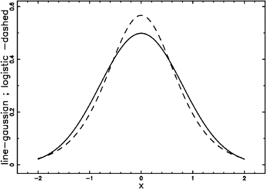
Figure 3: Normal PDF (full line) and logistic PDF as represented by Eq. (11) (dashed line) when $\sigma=0.8{{\mathrm{Mpc}}}/h$.

3.2 2D and 3D symmetry

We now analyze the astrophysical case in which the galaxies follow the logistic law along a perpendicular direction, $z$-axis, to a line along the $y$-axis (2D) and are randomly disposed in the $y$ direction. By analogy with the 3D case the galaxies will follow the logistic law in the $z$-direction and will be randomly generated in the $x$ and $y$ directions. In other words we realize a statistical equilibrium for galaxies with respect to a plane or to a line. Figures 4 and 5 report the computation of the 2D/3D PCF with a choice of parameters which give values of $\gamma_{{\mathrm{GG}}}$ and $r_{{\mathrm{G}}}$ similar to those observed, see Eq. (3).

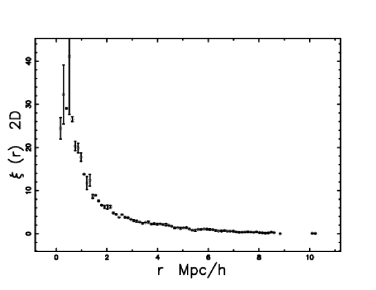
Figure 4: Values of the PCF for 200 galaxies generated according to the logistic PDF as represented by Eq. (11) in the $z$-direction; $\sigma=0.4{{\mathrm{Mpc}}}/h$, the length of the line of symmetry is 40 ${{\mathrm{Mpc}}}/h$ and $N_{{\mathrm{T}}}$= 20. The PCF as approximated by Eq. (3) has parameters $\gamma_{{\mathrm{GG}}}$=1.52 and $r_{{\mathrm{G}}}=5.27h^{-1}{{\mathrm{Mpc}}}$.

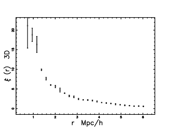
Figure 5: Values of the PCF for 200 galaxies generated according to to the logistic PDF as represented by Eq. (11) in the $z$-direction; $\sigma=0.1{{\mathrm{Mpc}}}/h$, the side of the plane of symmetry is 20 ${{\mathrm{Mpc}}}/h$ and $N_{{\mathrm{T}}}$= 30. The PCF as approximated by Eq. (3) has parameters $\gamma_{{\mathrm{GG}}}$=1.8 and $r_{{\mathrm{G}}}=4.97h^{-1}{{\mathrm{Mpc}}}$.

4 Astrophysical Applications

Up to now we have expressed all the distances in normalized units in which the unit is the averaged radius of the approximated circles/spheres which approximate the 2D/3D area/volume of a Voronoi cell. A second unit system is obtained multiplying the normalized distance $r_{u}$ by the averaged radius of the voids ,$\overline{R}$ , or $r=r_{u}\overline{R}$ ; this can be considered the physical space. A third unit system is connected with the redshift, $z$, which after Hubble (1929)

$$z=\frac{H_{0}D}{c}\quad,$$ (12)

where $H_{0}=100h\mathrm{\ km\ s}^{-1}\mathrm{\ Mpc}^{-1}$ , with $h=1$ when $h$ is not specified, $D$ is the distance in $Mpc$ and $c$ is the light velocity. In our framework

$$z=\frac{H_{0}\,r_{u}\overline{R}}{c}\quad$$ (13)

and this conversion defines the redshift space. Voronoi diagrams can model the local universe once two different calibrations are done. The first calibration is connected with the averaged effective radius of the voids. A first analysis of the Sloan Digital Sky Survey (SDSS) R7 catalog, see Pan et al. (2011), suggests $\overline{R}=18.23\,{{\mathrm{Mpc}}}/h$ as the averaged effective radius of the voids. A second analysis of the same catalog finds that the effective radii of the voids range from 5 to 135 Mpc/h and a first approximated evaluation gives $\overline{R}=70\,{{\mathrm{Mpc}}}/h$ , see Sutter et al. (2012). We therefore define an acceptable range of variability for the averaged effective radius of the voids

$$16.23\,{{\mathrm{Mpc}}}/h\leq\overline{R}\leq 70\,{{\mathrm{Mpc}}}/h\quad.$$ (14)

The theoretical averaged radius of the Voronoi volumes approximated by spheres should be comprised in this current range of variability; this is the first calibration. On adopting a practical point of view $\overline{R}$ will be fixed in such a way that the first minimum of the PCF is at 65 Mpc/h. A second calibration of the Voronoi diagrams originates from the PDF which models the statistics of the voids. A possible model for the observed statistics of the voids’ volumes as given by SDSS R7 is the Kiang function, see Kiang (1966),

$$H(x;c)=\frac{c}{\Gamma(c)}(cx)^{c-1}\exp(-cx),$$ (15)

with $c=2$, see Zaninetti (2012). Due to the fact that the PVT seeds are characterized by $c=5$ in the Kiang function we generate $N_{{\mathrm{s}}}$ seeds, in order to have $c=2$. see Zaninetti (2013). The points of a tessellation in 3D are of four types, depending on how many nearest neighbors in $ES$, the ensemble of seeds, they have. The name seeds derive from their role in generating cells. Basically we have two kinds of seeds , Poissonian and non Poissonian which generate the Poissonian Voronoi tessellation (PVT) and the non Poissonian Voronoi tessellation (NPVT). The Poissonian seeds are generated independently on the $X$, $Y$ and $Z$ axis in 3D through a subroutine which returns a pseudo-random real number taken from a uniform distribution between 0 and 1. This is the case most studied and for practical purposes, the subroutine RAN2 was used, see Press et al. (1992). The non Poissonian seeds can be generated in an infinite number of different ways: some examples of NPVT are reported in Zaninetti (2009), here the seeds are generated in order that the PDF in volumes follows a Kiang function with $c=2$. The algorithm that generates such seeds is reported in Section 3.3 of Zaninetti (2013). A point with exactly one nearest neighbor’s is in the interior of a cell, a point with two nearest neighbors is on the face between two cells, a point with three nearest neighbors is on an edge shared by three cells, and a point with four neighbors is a vertex where three cells meet. Following the nomenclature introduced by Okabe et al. (1992), we call the intersection between a plane and the PVT $V_{p}(2,3)$ and $V_{np}(2,3)$ the intersection between a plane and the NPVT. A discussion on how to extract the edges in 3D or the faces that in $V_{p}(2,3)$ and $V_{np}(2,3)$ become lines, can be found in Section 4.1 of Zaninetti (2010). We now explore two cases: the first case is a 2D cut or $V_{np}(2,3)$ on a 3D network which covers few voids and the second one is a cut which covers many voids.

4.1 Few voids

The 3D network of few voids can be visualized through the display of the edges, see Figure 6.

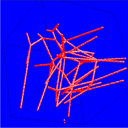
Figure 6: 3D visualization of the edges of few voids in NPVT. The parameters are $N_{{\mathrm{s}}}$ = 20, $side$ = 213 ${{\mathrm{Mpc}}}/h$ and $h=1$.

We now consider a 2D cut or $V_{np}(2,3)$ on the 3D NPVT network of faces, see Figure 7.

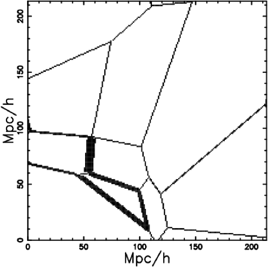
Figure 7: Cut or $V_{np}(2,3)$ on the $X-Y$ plane in the middle of the box of the NPVT faces.

We now compute the probability of having a galaxy according to the logistic law, see Eq. (11) , in the previous plane where $z$ is the distance from a face which in the 2D cut or $V_{np}(2,3)$ is a line . Figure 8 reports the values of the probability of having a galaxy in a 2D cut or $V_{np}(2,3)$ organized as a contour plot.

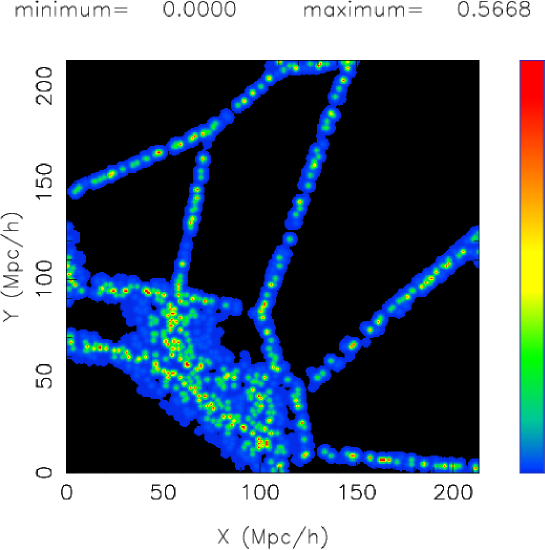
Figure 8: 2D map of the probability of having a galaxy. The Voronoi parameters are the same as in Figure 6 and $\sigma=0.8{{\mathrm{Mpc}}}/h$. The $X$ and $Y$ units are in ${{\mathrm{Mpc}}}/h$.

Figure 9 displays the PCF for large values of $r$ and Figure 10 the PCF for the full range of $r$; the first minimum exists but is not well defined.

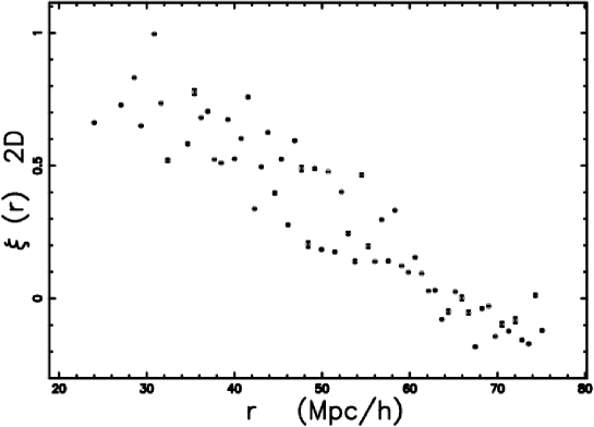
Figure 9: Values of the PCF for 10,000 galaxies generated according to the logistic PDF, Eq. (11), when $\sigma=0.8{{\mathrm{Mpc}}}/h$. Here the $z$ direction is perpendicular to the line which represents the face in a 2D cut or $V_{np}(2,3)$ . The distances are expressed in Mpc , the number of trials is 10 and the PCF is evaluated using Eq. (4). The position of the first minimum is at 67 Mpc/h.

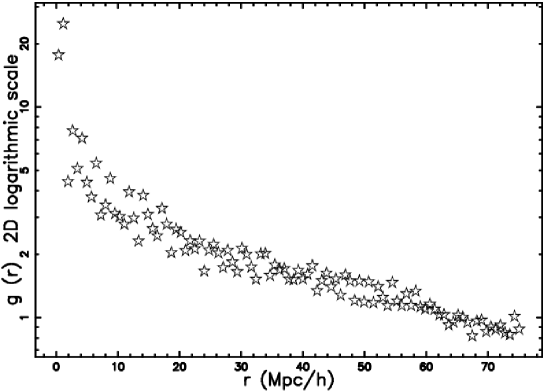
Figure 10: The same as Figure 9 but the vertical axis has a logarithmic scale.

4.2 Large Scale Structures

We start with a 3D box of $\approx$ 600 ${{\mathrm{Mpc}}}/h$ a side and we produce a 2D cut which is made by irregular polygons. On this 2D backbone we select 30,000 galaxies, see Figure 11.

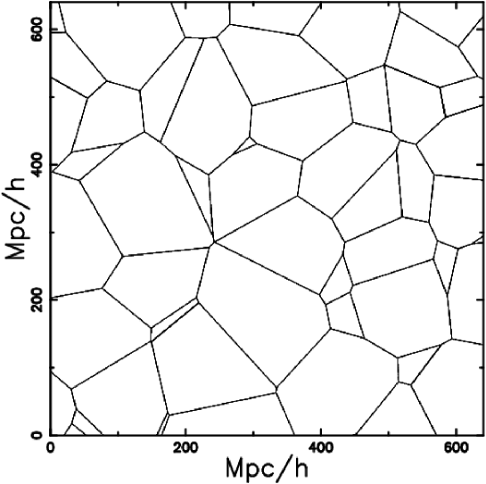
Figure 11: Network of 30,000 galaxies selected on the $X-Y$ plane in the middle of the box which crosses the NPVT faces.

We then compute the 2D PCF and the results is reported in Figure 12 together with the results of the PCF for 2dFVL, which is a nearly VL sample from 2dF Galaxy Redshift Survey (2dFGRS), see Croton et al. (2004). Our local minimum is at 65.17 Mpc/h and that of Figure 3 (red line) in Martínez et al. (2009) at 65 Mpc/h.

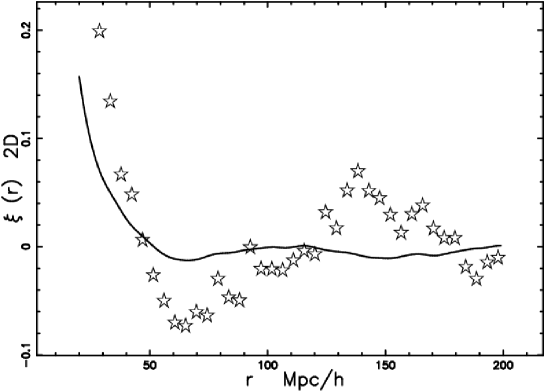
Figure 12: PCF for the 30,000 selected galaxies (empty stars) and the astronomical results of Martinez et al. (2009) (full line) for 2dFVL. The covered range is [0-200] Mpc/h and $N_{{\mathrm{T}}}$ =10.

5 Discussion

We now outline the differences between our approach and the usual model adopted by the astronomers. The model here adopted is based on the PCF of the vertexes of PVT which is developed in a 2D/3D Euclidean space. The standard approach to BAO conversely uses one of the 14 cosmological models available at the moment , see Sánchez et al. (2013). In the standard approach the first minimum going from the left to the right is reached at $z\approx 0.02\approx 65Mpc/h$. This observational fact allows us to derive $\overline{R}$ in our model. The same approximations are made in the void finding algorithms applied to galaxy survey data, which often use the spheres approximation, see Sutter et al. (2012); Nadathur and Hotchkiss (2013); Sutter et al. (2013). This approximation is valid when the thickness of the surface which contains the galaxies , $\sigma$ according to eqn. (11), is smaller than $\overline{R}$. A theoretical explanation for the variability of the averaged radius of the cosmic voids is perhaps due to the absence of analytical results for the $V_{p}(2,3)$ problem. A new analytical result for the radius of the cell in $V_{p}(2,3)$ in the PVT case is

$$f(r,b)=AG^{4,1}_{3,5}\left({\frac{100}{9}}{\frac{{\pi}^{2}{r}^{6}}{{b}^{6}}}\Big{|}^{5/6,1/6,1/2}_{7/3,2/3,1/3,0,{\frac{17}{6}}}\right)(\frac{1}{b})^{2}$$ (16)

$$\quad 0\leq r\leq b,$$

where

$$A=\frac{2}{3}{\it K}\sqrt[6]{3}\sqrt[3]{10}\sqrt[3]{\pi}r\quad,$$ (17)

${K}$ is a constant, $K=1.6485$, $r$ is the radius of the cell, $b$ the scale and the Meijer $G$-function is defined as in Meijer (1936, 1941); Olver et al. (2010); see Zaninetti (2012) for more details. Figure 13 reports the statistics of the radius of the cells $V_{p}(2,3)$ for the PVT case as well the frequencies of the effective radius of SDSS DR7. In the previous figure the $\chi^{2}$ is computed according to the formula

$$\chi^{2}=\sum_{i=1}^{n}\frac{(T_{i}-O_{i})^{2}}{T_{i}},$$ (18)

where $n$ is the number of bins, $T_{i}$ is the theoretical value, and $O_{i}$ is the experimental value represented by the frequencies. The merit function $\chi_{red}^{2}$ is evaluated by

$$\chi_{red}^{2}=\chi^{2}/NF\quad,$$ (19)

where $NF=n-k$ is the number of degrees of freedom, $n$ is the number of bins, and $k$ is the number of parameters, in our case 2.

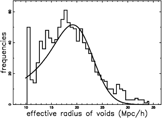
Figure 13: Histogram (step-diagram) of the effective radius of SDSS DR7 with a superposition of the PDF in radius of the PVT 2D cells as represented by Eq. (5). The parameters are $n$=40, $k$=2,$b$= 34.7/h Mpc , $\chi^{2}$=98 and $\chi_{red}^{2}$=2.6.

The averaged effective radius is $\overline{r}$= 18.23 Mpc/h but the averaged radius of the cosmic voids approximated by spheres is $\overline{R}$= 22.6 Mpc/h. The previous formula contains the Meijer $G$-function which does not have an easy numerical implementation. An approximate PDF for the radius of the cell in $V_{p}(2,3)$ in the PVT case, eqn. (5) can be found in the framework of the generalized gamma PDF, see Evans et al. (2000) ,

$$G(x;a,b,c)=\frac{c{b}^{{\frac{a}{c}}}{x}^{a-1}{{\rm e}^{-b{x}^{c}}}}{\Gamma\left({\frac{a}{c}}\right)}\quad.$$ (20)

The three parameters $a$ , $b$ and $c$ can be found through the Levenberg–Marquardt method ( subroutine MRQMIN in Press et al. (1992))

$$f(r,b)_{app}=\frac{9.291\,\left({\frac{r}{b}}\right)^{1.77}{{\rm e}^{-28.35\,\left({\frac{r}{b}}\right)^{8.44}}}}{b}\quad,$$ (21)

and figure 14 reports the analytical PDF and the approximate PDF.

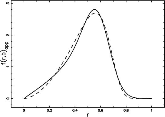
Figure 14: The analytical PDF, $f(r,b)$, (full line) and and the approximate $f(r,b)_{app}$ (dashed line).

This approximate PDF gives a relative error of $0.5\%$ in the evaluation of the averaged value.

6 Conclusions

The BAO are here analyzed in the framework of PVT and NPVT. A first test for the PCF is done on the 2D/3D vertexes of PVT. Figures 1 and 2 compare the well known mathematical results with our simulation. The PCF of 2D and 3D vertexes in PVT presents a first minimum at $r/\bar{R}\approx 1$ in 2D and at $r/\bar{R}\approx 1.4$ in 3D. The applications to the local universe are done in the framework of galaxies distributed according to an auto-gravitating medium in respect to the faces of the irregular Voronoi’s polyhedrons, see the PDF 11. We first tested the logistic PDF for a vertical distribution of galaxies in 2D/3D in order to reproduce the observed small scale behavior of the PCF, see Figure 4 in 2D and Figure 5 in 3D. The analysis of the oscillations of the PCF in the local universe are split in two. We firstly analyzed the case of a 2D cut or $V_{np}(2,3)$ which covers few voids in the presence of an auto-gravitating medium with a given value of variance $\sigma=0.8{{\mathrm{Mpc}}}/h$. In this 2D cut or $V_{np}(2,3)$ the PCF presents the first minimum at $r\approx 67{{\mathrm{Mpc}}}/h$ when $\bar{R}$ = 42 Mpc. The second case is represented by a 2D cut or $V_{np}(2,3)$ which covers $\approx 50$ voids and the first minimum is at $r\approx 65.17{{\mathrm{Mpc}}}/h$ when $\bar{R}$ = 54 Mpc/h. The PCF turns out to be similar to the behavior of 2dFVL sample , see Figure 3 in Martínez et al. (2009), where the first local minimum is reached at $\approx$ 65 Mpc/h. Here we have provided an NPVT environment and distances of the astrophysical simulations expressed in Mpc/h. According to the previous results the distances of the PCF should be expressed in averaged radius units rather than Mpc/h . As a practical example when $\bar{R}$ = 54 Mpc/h is used as a calibrating value in our simulation, the first local minimum of the PCF should be at 1.2 universal units according to the data of the 2dFVL sample, see Sec. 4.2.

References

- Allen and Tildesley (1987) Allen, M. P. and Tildesley, D. J. (1987), Computer simulation of liquids, Oxford, NY: Oxford University Press.
- Angulo et al. (2008) Angulo, R. E., Baugh, C. M., Frenk, C. S., and Lacey, C. G. (2008), “The detectability of baryonic acoustic oscillations in future galaxy surveys,” MNRAS , 383, 755–776.
- Balakrishnan (1991) Balakrishnan, N. (1991), Handbook of the Logistic Distribution, New York: Taylor & Francis.
- Bertin (2000) Bertin, G. (2000), Dynamics of Galaxies, Cambridge: Cambridge University Press.
- Croton et al. (2004) Croton, D. J., Colless, M., Gaztañaga, E., and Baugh, C. M. (2004), “The 2dF Galaxy Redshift Survey: voids and hierarchical scaling models,” MNRAS , 352, 828–836.
- Eisenstein et al. (2005) Eisenstein, D. J., Zehavi, I., Hogg, D. W., Scoccimarro, R., Blanton, M. R., and Nichol, R. C. e. a. (2005), “Detection of the Baryon Acoustic Peak in the Large-Scale Correlation Function of SDSS Luminous Red Galaxies,” ApJ , 633, 560–574.
- Evans et al. (2000) Evans, M., Hastings, N., and Peacock, B. (2000), Statistical Distributions - third edition, New York: John Wiley & Sons Inc.
- Hansen, J. P. and McDonald, I. R. (1986) Hansen, J. P. and McDonald, I. R. (1986), Theory of simple liquids, New York: Academic Press.
- Heinrich and Muche (2008) Heinrich, L. and Muche, L. (2008), “Second-order properties of the point process of nodes in a stationary Voronoi tessellation.” Math. Nachr., 281, 350–375.
- Hubble (1929) Hubble, E. (1929), “A Relation between Distance and Radial Velocity among Extra-Galactic Nebulae,” Proceedings of the National Academy of Science, 15, 168–173.
- Johnson et al. (1995) Johnson, N. L., Kotz, S., and Balakrishnan, N. (1995), Continuous univariate distributions. Vol. 2. 2nd ed., New York: Wiley .
- Kiang (1966) Kiang, T. (1966), “Random Fragmentation in Two and Three Dimensions,” Z. Astrophys. , 64, 433–439.
- Martínez et al. (2009) Martínez, V. J., Arnalte-Mur, P., Saar, E., de la Cruz, P., Pons-Bordería, M. J., Paredes, S., Fernández-Soto, A., and Tempel, E. (2009), “Reliability of the Detection of the Baryon Acoustic Peak,” ApJ , 696, L93–L97.
- McQuarrie (1976) McQuarrie, D.-A. (1976), Statistical Mechanics, New York: Harper and Row.
- Mehta et al. (2011) Mehta, K. T., Seo, H.-J., Eckel, J., Eisenstein, D. J., Metchnik, M., Pinto, P., and Xu, X. (2011), “Galaxy Bias and Its Effects on the Baryon Acoustic Oscillation Measurements,” ApJ , 734, 94.
- Meijer (1936) Meijer, C. (1936), “Über Whittakersche bzw. Besselsche Funktionen und deren Produkte.” Nieuw Arch. Wiskd., 18, 10–39.
- Meijer (1941) — (1941), “Multiplikationstheoreme für die Funktion .” Proc. Akad. Wet. Amsterdam, 44, 1062–1070.
- Nadathur and Hotchkiss (2013) Nadathur, S. and Hotchkiss, S. (2013), “A self-consistent public catalogue of voids and superclusters in the SDSS Data Release 7 galaxy surveys,” ArXiv e-prints.
- Okabe et al. (1992) Okabe, A., Boots, B., and Sugihara, K. (1992), Spatial tessellations. Concepts and Applications of Voronoi diagrams, Chichester, New York: Wiley.
- Okabe et al. (2000) Okabe, A., Boots, B., Sugihara, K., and Chiu, S. (2000), Spatial tessellations. Concepts and Applications of Voronoi diagrams, 2nd ed., Chichester, New York: Wiley.
- Olver et al. (2010) Olver, F. W. J. e., Lozier, D. W. e., Boisvert, R. F. e., and Clark, C. W. e. (2010), NIST handbook of mathematical functions., Cambridge: Cambridge University Press. .
- Padmanabhan (2002) Padmanabhan, P. (2002), Theoretical astrophysics. Vol. III: Galaxies and Cosmology, Cambridge, MA: Cambridge University Press.
- Pan et al. (2011) Pan, D. C., Vogeley, M. S., Hoyle, F., Choi, Y.-Y., and Park, C. (2011), “Cosmic Voids in Sloan Digital Sky Survey Data Release 7,” ArXiv e-prints:1103.4156.
- Press et al. (1992) Press, W. H., Teukolsky, S. A., Vetterling, W. T., and Flannery, B. P. (1992), Numerical Recipes in FORTRAN. The Art of Scientific Computing, Cambridge: Cambridge University Press.
- Rohlfs (1977) Rohlfs, K. (ed.) (1977), Lectures on density wave theory, vol. 69 of Lecture Notes in Physics, Berlin Springer Verlag.
- Sánchez et al. (2013) Sánchez, E., Alonso, D., Sánchez, F. J., García-Bellido, J., and Sevilla, I. (2013), “Precise measurement of the radial baryon acoustic oscillation scales in galaxy redshift surveys,” MNRAS , 434, 2008–2019.
- Seo and Eisenstein (2007) Seo, H.-J. and Eisenstein, D. J. (2007), “Improved Forecasts for the Baryon Acoustic Oscillations and Cosmological Distance Scale,” ApJ , 665, 14–24.
- Seo et al. (2012) Seo, H.-J., Ho, S., White, M., Cuesta, A. J., Ross, A. J., and Saito, S. (2012), “Acoustic Scale from the Angular Power Spectra of SDSS-III DR8 Photometric Luminous Galaxies,” ApJ , 761, 13.
- Spitzer (1942) Spitzer, Jr., L. (1942), “The Dynamics of the Interstellar Medium. III. Galactic Distribution.” ApJ , 95, 329.
- Stoyan and Stoyan (1990) Stoyan, D. and Stoyan, H. (1990), “Exploratory data analysis for planar tessellations: Structural analysis and point process methods.” Appl. Stochastic Models Data Anal., 6, 13–25.
- Sutter et al. (2012) Sutter, P. M., Lavaux, G., Wandelt, B. D., and Weinberg, D. H. (2012), “A Public Void Catalog from the SDSS DR7 Galaxy Redshift Surveys Based on the Watershed Transform,” ApJ , 761, 44.
- Sutter et al. (2013) — (2013), “A response to arXiv:1310.2791: A self-consistent public catalogue of voids and superclusters in the SDSS Data Release 7 galaxy surveys,” ArXiv e-prints,1310.5067.
- Szalay et al. (1993) Szalay, A. S., Broadhurst, T. J., Ellman, N., Koo, D. C., and Ellis, R. S. (1993), “Redshift Survey with Multiple Pencil Beams at the Galactic Poles,” Proceedings of the National Academy of Science, 90, 4853–4858.
- Totsuji and Kihara (1969) Totsuji, H. and Kihara, T. (1969), “The Correlation Function for the Distribution of Galaxies,” PASJ , 21, 221.
- White et al. (2010) White, M., Pope, A., Carlson, J., Heitmann, K., Habib, S., Fasel, P., Daniel, D., and Lukic, Z. (2010), “Particle Mesh Simulations of the Ly Forest and the Signature of Baryon Acoustic Oscillations in the Intergalactic Medium,” ApJ , 713, 383–393.
- Yarnell et al. (1973) Yarnell, J. L., Katz, M. J., Wenzel, R. G., and Koenig, S. H. (1973), “Structure Factor and Radial Distribution Function for Liquid Argon at 85 degree K,” Phys. Rev. A, 7, 2130–2144.
- Zaninetti (2009) Zaninetti, L. (2009), “Poissonian and non-Poissonian Voronoi diagrams with application to the aggregation of molecules,” Phys. Lett. A , 373, 3223–3229.
- Zaninetti (2010) — (2010), “ A geometrical model for the catalogs of galaxies ,” Revista Mexicana de Astronomia y Astrofisica, 46, 115–134.
- Zaninetti (2012) — (2012), “New Analytical Results for Poissonian and non-Poissonian Statistics of Cosmic Voids,” Revista Mexicana de Astronomia y Astrofisica, 48, 209–222.
- Zaninetti (2013) — (2013), “ Chord distribution along a line in the local Universe ,” Revista Mexicana de Astronomia y Astrofisica, 49, 117–126.
- Zehavi et al. (2004) Zehavi, I., Weinberg, D. H., Zheng, Z., Berlind, A. A., Frieman, J. A., and Scoccimarro, R. (2004), “On Departures from a Power Law in the Galaxy Correlation Function,” ApJ , 608, 16–24.
- Zhan and Knox (2006) Zhan, H. and Knox, L. (2006), “Baryon Oscillations and Consistency Tests for Photometrically Determined Redshifts of Very Faint Galaxies,” ApJ , 644, 663–670.