Using the $s$-Ensemble to Probe Glasses Formed by Cooling and Aging

Abstract

From length scale distributions characterizing frozen amorphous domains, we relate the $s$-ensemble method with standard cooling and aging protocols for forming glass. We show that in a general class of models, where space-time scaling is in harmony with that of experiment, the domain size distributions obtained with the $s$-ensemble are identical to those obtained through cooling or aging, but the computational effort for applying the $s$-ensemble is generally many orders of magnitude smaller than that of straightforward numerical simulation of cooling or aging.

Through biasing statistics of trajectory space, the so-called “$s$-ensemble” method, non-equilibrium phase transitions emerge between ergodic liquid-like states and dynamically inactive glass-like states. This class of transitions are found in idealized lattice models Merolle et al. (2005); Garrahan et al. (2007) and in simulations of atomistic models Hedges et al. (2009); Speck and Chandler (2012); Speck et al. (2012). In the latter case, it affords a systematic computational means of preparing exceptionally stable glass-states states Jack et al. (2011). This Letter draws the conclusion that the $s$-ensemble transition coincides with the physical glass transition reviews , and the ensemble of its inactive states are those of natural structural glass. Specifically, we derive correspondence between spatial correlations in the $s$-ensemble glass with those in the glass produced with finite-rate cooling or aging. The correspondence provides a basis for an extraordinarily efficient route for preparing structural glass with molecular simulations.

Space-time structure of glass-forming liquids. To begin, it is helpful to consider Figs. 1a and 1b, which render trajectories of a two-dimensional $5\times 10^{4}$-particle system in a fashion that extends the approach of Ref. Keys et al. (2011). The system is a liquid mixture at a temperature that is 80% below that of the onset temperature, $T_{\mathrm{o}}$ Keys et al. (2011); Garrahan and Chandler (2003); Elmatad et al. (2009, 2010); Note (1), and the trajectory runs for an observation time $t_{\mathrm{obs}}\approx 10\,\tau$. Here, $\tau$ stands for the equilibrium structural relaxation time. It is about $10^{5}$ integration steps at this particular temperature, and $t_{\mathrm{obs}}$, being 10 times longer, provides ample opportunity to observe the nature of dynamic heterogeneity in the system.

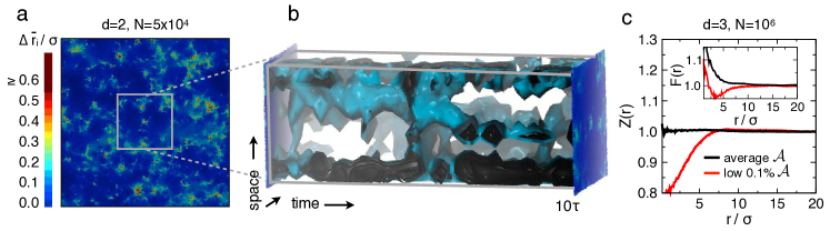
Figure 1: Soft spots and space-time bubbles. (a) Burnished excitations for the $d=2$ supercooled WCA liquid mixture Keys et al. (2011), with $\Delta\bar{r}_{i}=[|\bar{\mathbf{r}}_{i}(\Delta t)-\bar{\mathbf{r}}_{i}(0)|]_{\mathrm{iso}}$. (b) Excitation lines for a subsection of the system shown in (a). (c) The functions $Z(r)$ and $F(r)$ demonstrating correlation holes for inactive subsystems of a supercooled $d=3$ WCA liquid mixture Hedges et al. (2007).

Most motions in glass-forming liquids are irrelevant vibrations, and the amplitudes of most of those vibrations are similar in size to typical enduring displacements Keys et al. (2011). Irrelevant vibrations can be filtered out by focusing on inherent structures Stillinger and Weber (1982). The set of particle positions at time $t$, $\{\mathbf{r}_{i}(t)\}$, evolves by molecular dynamics; the inherent structure, $\{\bar{\mathbf{r}}_{i}(t)\}$, is the position of the potential-energy minimum closest to $\{\mathbf{r}_{i}(t)\}$. The renderings in Fig. 1 refer to $[a(\mathbf{r},t)]_{\mathrm{iso}}$, where

$$a(\mathbf{r},t)=\sum_{i=1}^{N}|\bar{\mathbf{r}}_{i}(t+\Delta t)-\bar{\mathbf{r}}_{i}(t)|\,\delta(\mathbf{r}-\bar{\mathbf{r}}_{i}(t))\,.$$ (1)

Here, we take $\Delta t$ to be $10^{3}$ integration steps, which is roughly the average time to complete an enduring displacement of one atomic diameter Keys et al. (2011), and $[\cdots]_{\mathrm{iso}}$ indicates iso-configurational averaging, which averages many trajectories of length $\Delta t$, all starting from the same configuration Widmer-Cooper et al. (2004). Particles colored red in Fig. 1a are those for which the iso-configuration averaged $\bar{\mathbf{r}}_{i}(\Delta t)$ is more than $0.6\,\sigma$ from $\bar{\mathbf{r}}_{i}(0)$, where $\sigma$ is a particle diameter. Smaller enduring displacements are colored by interpolating between red and blue, as noted in the color scale. The figure thus shows that enduring displacements occurring over a short period of time, $\Delta t$, take place in sparse localized regions of space. These regions are the excitations Keys et al. (2011) in an otherwise rigid material.

Similar pictures illustrating arrangements of enduring displacements are found without iso-configuration averaging. See Fig. 1 of Ref. Keys et al. (2011) and also Media 1 of Ref. Keys et al. (2011). Iso-configurational averaging serves to burnish those pictures Note (2). Without that averaging, localized excitations are already evident but more irregular. Importantly, the excitations, often referred to as soft spots Manning and Liu (2011), change little in size as the liquid is cooled, and further, there are no inter-excitation correlations at equal times Keys et al. (2011).

Correlations develop over time through dynamics, which is illustrated with Fig. 1b. That picture shows constant-value surfaces of $[a(\mathbf{r},t)]_{\mathrm{iso}}$. The surfaces form connected tubes or lines in space time – excitation lines Garrahan and Chandler (2002) – indicating that excitations facilitate birth (and death) of adjacent excitations. Larger amplitude fluctuations of the surface occur less frequently than smaller amplitude fluctuations, indicating that the facilitated dynamics is hierarchical Palmer et al. (1984). Lowering temperature reduces the number of excitations or soft spots, which reduces the probability that soft spots can connect, which reduces the rate at which the system can relax.

This behavior is found consistently in glass-forming liquids for all temperatures below the onset, i.e., $T<T_{\mathrm{o}}$ Keys et al. (2011). Throughout this regime, it is characterized by simple equations for space-time scaling and for the equilibrium distribution of distances between neighboring soft spots, $P_{\mathrm{eq}}(\ell)$:

$$\ell/\sigma=(\tau_{\ell}/\tau_{\mathrm{o}})^{1/\tilde{\beta}\gamma}\,.$$ (2)

and

$$P_{\mathrm{eq}}(\ell)=\ell_{\mathrm{eq}}^{-1}\exp(-\ell/\ell_{\mathrm{eq}})\,,\quad\ell_{\mathrm{eq}}=\sigma\exp(\tilde{\beta}/d_{\mathrm{f}})\,,$$ (3)

Here, $\tilde{\beta}=J_{\sigma}/T-J_{\sigma}/T_{\mathrm{o}}$, where $J_{\sigma}$ is the energy of an excitation with enduring displacements of the characteristic structural length, $\sigma$, $1/\tau_{\ell}$ is the relaxation rate on length scale $\ell$, $d_{\mathrm{f}}$ is the fractal dimensionality of dynamic heterogeneity, and $\gamma$ is the proportionality constant for logarithmic growth of excitation energy with respect to length scale Note (3). The parabolic law Garrahan and Chandler (2003); Elmatad et al. (2009); Keys et al. (2011), $\tau=\tau_{\mathrm{o}}\exp(\tilde{\beta}^{2}\gamma/d_{\mathrm{f}})$, follows from space-time scaling, Eq. (2), evaluated at $\ell=\ell_{\mathrm{eq}}$.

Contributions to $P_{\mathrm{eq}}(\ell)$ with short inter-excitation lengths, $\ell<\ell_{\mathrm{eq}}$, come from regions with excitation lines that connect and reorganize. Contributions with $\ell\gg\ell_{\mathrm{eq}}$ come from regions of rigidity – the empty regions of Fig. 1b, so-called “bubbles” in space-time Garrahan and Chandler (2002). When the liquid transforms into glass, the temporal extents of those bubbles grow to very long times, and excitation lines rarely or never touch, yielding a striped structure of trajectory space Keys et al. (2013). In that case, excitations are no longer uncorrelated, and a non-equilibrium correlation length, $\ell_{\mathrm{ne}}$, gives the average or most probable separation of excitation lines.

Figure 1c shows that the equilibrium glass-forming liquid already contains the seeds of this non-equilibrium correlation length. Specifically, for a $10^{6}$-particle WCA liquid mixture Hedges et al. (2007) in $d=3$ at $T=0.7\,T_{\mathrm{o}}$, Fig. 1c contrasts the equilibrium concentration of excitations with that surrounding a dynamically inactive sub-volume. The trajectory length is $t_{\mathrm{obs}}=50\tau\approx 10^{3}\Delta t$. The net dynamical activity in a sub-volume $\Delta v$ is $\int_{0}^{t_{\mathrm{obs}}}dt\int_{\Delta v}d\mathbf{r}\,a(\mathbf{r},t)$. For Fig. 1c, we have partitioned the total volume $V$ into cubes, each of size $\Delta v=125V/N$, and computed $Z(r)=\langle a(\mathbf{r})\rangle_{\Delta v}/a$. Here, $a$ is the equilibrium average of $a(\mathbf{r},t)$, and $\langle\cdots\rangle_{\Delta v}$ is that average conditioned on a low activity in the sub-volume at the origin. Similarly, we have computed the radial distribution of mobility, $F(r)=\langle a(\mathbf{r})\rangle_{0}/ag(r)$, where $g(r)N/V$ is the mean particle density at $\mathbf{r}$ given a particle is at the origin and $\langle\cdots\rangle_{0}$ is the equilibrium average given a particle at the origin has just then completed an enduring displacement of at least $0.3\,\sigma$. The red lines of Fig. 1c refer to the 0.1% least active sub-volumes. For $F(r)$, that means the central displacing particle is within such a low-activity sub-volume. The equilibrium $Z(r)$ exhibits no structure, and the equilibrium $F(r)$ decays over the length scale of a single excitation. In contrast, the atypical low-activity functions show significant anti-correlation between neighboring excitations.

Preparing glassy states. The statistical weight for these low-activity regions are enhanced by shifting to a non-equilibrium $s$-ensemble distribution, $P_{s}[x(t)]\propto P_{0}[x(t)]\exp(-s{\mathcal{A}}[x(t)])$ Garrahan et al. (2007); Hedges et al. (2009); Speck and Chandler (2012); Lecomte et al. (2007). Here, $P_{0}[x(t)]$ is the equilibrium distribution functional for trajectories $x(t)$ of length $t_{\mathrm{obs}}$, and ${\mathcal{A}}[x(t)]$ is the net dynamical activity Note (4),

$${\mathcal{A}}[x(t)]=\int_{V}d\mathrm{r}\int_{0}^{t_{\mathrm{obs}}}dt\,\,a(\mathrm{r},t)\,.$$ (4)

For an ergodic equilibrium system, ${\mathcal{A}}=t_{\mathrm{obs}}Va$. Deviations from this equilibrium value are measures of non-ergodic non-equilibrium behavior. Time integrals of other quantities, not just the activity as in (4), can also serve as suitable order parameters to distinguish ergodic and non-ergodic behavior. Time integration is the crucial feature. Fluctuations are then intimately related to the behavior of time correlators.

Remarkably, for systems at $T<T_{\mathrm{o}}$, the marginal equilibrium distribution for ${\mathcal{A}}$ exhibits fat tails at low activity Merolle et al. (2005), so that the non-equilibrium mean, $\langle\mathcal{A}\rangle_{s}$, changes abruptly around a transition value of $s$. For $s<s^{*}$, the material is a normal melt, and for $s>s^{*}$, the material is an inactive amorphous phase – a glass. The abrupt change tends to a discontinuity as $Nt_{\mathrm{obs}}\rightarrow\infty$. The glass transition in the $s$-ensemble is thus a first-order transition Garrahan et al. (2007); Hedges et al. (2009); Speck and Chandler (2012).

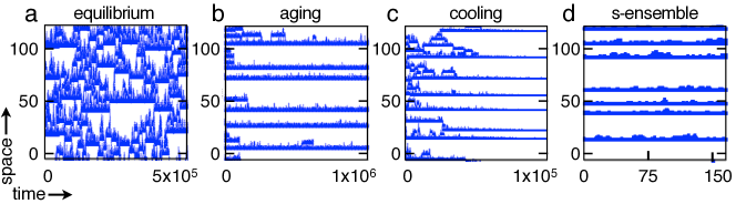
Figure 2: Trajectories of excitations in the East model. (a) Equilibrium dynamics for $T=0.45$ over a time scale spanning about 50 structural relaxation times at that temperature. (b) Aging dynamics after a quench from $T=1$ to $T=0.25$. (c) Cooling at a rate $\nu=10^{-5}$. (d) Trajectory from the $s$-ensemble at $T=0.72$ and $s>s^{*}\approx 10^{-2}$, trajectories running for about 1/2 a structural relaxation time at that temperature.

Even more remarkably, the transition can be obtained with $t_{\mathrm{obs}}$ much shorter than time scales required to produce glass from standard cooling protocols. By cooling at a rate $\nu$, a glass transition occurs at the temperature $T_{\mathrm{g}}$, where $\nu^{-1}\approx|d\tau/dT|_{T=T_{\mathrm{g}}}$. The time scale for that process is $\tau_{\mathrm{g}}=\tau(T_{\mathrm{g}})$. The transition freezes excitations separated by the non-equilibrium length, $\ell_{\mathrm{ne}}=\ell_{\mathrm{eq}}(T_{\mathrm{g}})$. From Eq. (2), $\ell_{\mathrm{ne}}/\sigma=(\tau_{\mathrm{g}}/\tau_{\mathrm{o}})^{1/\tilde{\beta}_{\mathrm{g}}\gamma}$. This length must be large if the glass persists for long times. Thus, in view of Eq. (3), $\tilde{\beta}_{\mathrm{g}}>1$. Typically, $\tau_{\mathrm{g}}>10^{10}\tau_{\mathrm{o}}$ and $\ell_{\mathrm{ne}}\gtrsim 10\sigma$.

On the other hand, with the $s$-ensemble, the same large non-equilibrium length can be obtained with any positive value of $\tilde{\beta}$. In that case, from Eq. (2), $\ell_{\mathrm{ne}}/\sigma=(t_{\mathrm{obs}}/\tau_{\mathrm{o}})^{1/\tilde{\beta}\gamma}$. As such,

$$t_{\mathrm{obs}}/\tau_{\mathrm{o}}=(\tau_{\mathrm{g}}/\tau_{\mathrm{o}})^{\tilde{\beta}/\tilde{\beta}_{\mathrm{g}}}\,.$$ (5)

The ratio $\tilde{\beta}/\tilde{\beta}_{\mathrm{g}}$ can be much smaller than 1. In practice, $\tilde{\beta}/\tilde{\beta}_{\mathrm{g}}\approx 1/10$. Thus, the simulation time required to prepare a glassy state in the $s$-ensemble, $t_{\mathrm{obs}}$, is many orders of magnitude shorter than the time to prepare glass by straightforward cooling, $\tau_{\mathrm{g}}$.

Illustration with the East model. Equation 5 follows from well-tested scaling relationships, and there is some empirical evidence that glasses produced with the $s$-ensemble do indeed coincide with natural structural glass Jack et al. (2011); Limmer and Chandler (2013). Nevertheless, this relationship is not yet tested explicitly. Here, we do so for the East model Jäckle and Eisinger (1991), the simplest of models consistent with phenomenology of structural glasses and glass formers Elmatad et al. (2009); Elmatad and Keys (2012); Keys et al. (2013).

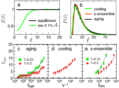
Figure 3: Distributions of East-model glasses. (a) The relative concentration of excitations a distance $\ell$ from one of the least active sub-regions in the equilibrium model at temperature $T=0.5$ (b) Distributions of domain lengths $P(\ell)$ for systems aged, cooled and driven with s, all designed to yield $\ell_{\mathrm{ne}}\approx 10$. Here, $\ell$ represents the distance between frozen excitations (called “super-spins”Sollich and Evans (2003)). Aging was done at $T=0.25$ for $t_{\mathrm{age}}=2.5\times 10^{5}$ after quenching from $T=0.4$. Cooling to $T=0$ was done with a cooling rate of $\nu=10^{-6}$. s-enemble trajectories were carried out at $T=0.72$ for a time duration of $t_{\mathrm{obs}}=320$. (c-e) Growth of $\ell_{\mathrm{ne}}$ as a function of relevant time variables. Dashed lines in (c) refer to $\ell_{\mathrm{ne}}=(t_{\mathrm{age}}/\tau_{\mathrm{o}})^{1/\tilde{\beta}\gamma}$; dashed line in (d) refers to $\ell_{\mathrm{eq}}(T_{\mathrm{g}})$; dashed lines in (e) refer to $\ell_{\mathrm{ne}}=(t_{\mathrm{obs}}/\tau_{\mathrm{o}})^{1/\tilde{\beta}\gamma}$.

In brief, the East model consists of a $d=1$ lattice with $N$ sites, each with variables $n_{i}=0,1$. The equilibrium concentration of excitations is $\langle n_{i}\rangle=c$. At low temperatures, $c\sim\exp(-1/T)$. (We take 1 as the energy scale and length scale for the model.) Sites with $n_{i}=1$ can facilitate a spin flip at the adjacent site $n_{i+1}$. The corresponding transition rates are given for a site $i$ by $k_{i,0\rightarrow 1}=n_{i-1}c/(1-c)$ and $k_{i,1\rightarrow 0}=n_{i-1}$. The dynamics of this model is hierarchical Jäckle and Eisinger (1991); Sollich and Evans (2003). Its structural relaxation slows by twelve orders of magnitude as $T$ decreases from 1 to 0.2 Ashton et al. (2005), it obeys space-time scaling of Eq. (2) and the parabolic law with $\gamma\approx 1/2\ln 2$ Ashton et al. (2005); Aldous and Diaconis (2002); Chleboun et al. (2013). (A different value of $\gamma$ applies for aging regimes Note (5).) An equilibrium trajectory of the model is shown in Fig. 2a. Three protocols for preparing non-equilibrium glass states are illustrated in Figs. 2b, 2c and 2d.

In the first, aging, the model is initially equilibrated at $T=1$ and then instantly quenched to $T=0.25$, after which it runs at that the low temperature for times $t_{\mathrm{age}}$, where $\tau(1)\ll t_{\mathrm{age}}\ll\tau(0.25)\approx 3\times 10^{9}$. During the time $t_{\mathrm{age}}$, the system can relax domains that are smaller than a characteristic length Sollich and Evans (2003); Keys et al. (2013) $\ell_{\mathrm{ne}}=\left(t_{\mathrm{age}}/\tau_{\mathrm{o}}\right)^{1/\tilde{\beta}\gamma}$, with $\tilde{\beta}\approx 3$. We use $t_{\mathrm{age}}\approx 10^{6}$ so as to produce an average non-equilibrium spacing between excitations of about 10.

In the second, cooling, the model is equilibrated at a temperature $T=1$ and then cooled to zero temperature at a rate of $\nu=10^{-5}$. A glass transition occurs at the stage where $1/\nu\approx|d\tau/dT|$, which gives $T_{g}\approx 0.48$ and thus $\ell_{\mathrm{ne}}\approx 10$ and $\tau_{\mathrm{g}}\approx 10^{6}$. In other words, excitations in the glass are frozen in with a typical spacing of about 10, and the time scale to create the material is about $10^{6}$.

The third case, the $s$-ensemble protocol, produces a similar glass in a much shorter time. A similar inter-excitation distance is targeted with trajectories run at $T=0.72$ for which $\tau\approx 300$ and $\tilde{\beta}\approx 0.3$. The glass transition from the cooling protocol occurs at $\tilde{\beta}_{\mathrm{g}}\approx 1/(1/2)-1=1$. Accordingly, from Eq. (5), the $s$-ensemble transition for trajectories at $T=0.72$ produces the glass with $\ell_{\mathrm{ne}}$ when $t_{\mathrm{obs}}\approx 100$. To apply the $s$-ensemble, we use the total number of enduring kinks as a measure of dynamical activity. An enduring kink at site $i$ is a change in $n_{i}$ that persists for at least a mean exchange time Elmatad and Keys (2012). At $T=0.72$ and $t_{\mathrm{obs}}\approx 100$, for system size $N$ chosen, the $s$-ensemble glass transition occurs at $s^{*}\approx 10^{-2}=O(1/N)$ Bodineau et al. (2012) (see Supplemental Material).

Figure 3 compares the non-equilibrium correlation lengths and distribution functions for the three different preparation protocols. It also shows $Z(\ell)$, which is the relative concentration of enduring kinks a distance $\ell$ from the 0.1% least-active domains of the equilibrium East model. It exhibits a correlation hole in a fashion similar to the analogous $Z(r)$ in the WCA mixture, Fig. 1. The East model thus illustrates how preparation of glass, which necessarily requires long physical times, can be accomplished in simulation in much shorter times through application of the $s$-ensemble. Equation (5) provides the key for understanding prior successes in preparing glassy states through applications of the $s$-ensemble in atomistic models. However, if the simulation box size, $L$, is smaller than target non-equilibrium length, the $s$-ensemble method prepares a distribution of glassy states, all of which correspond to inactive domains in glasses with $\ell_{\rm ne}>L$.

Natural dynamics changes $\ell$ continuously, and at the point where the system falls out of equilibrium $\ell_{\rm ne}=\ell_{\rm eq}$. The equilibrium length, $\ell_{\rm eq}=\langle\ell\rangle$, is equivalent to $a$ or $c$. Because the length scale changes continuously as a glass former falls out of equilibrium, the glass transition has the appearance of a second-order transition. However, the time-integrated order parameters, the distribution of $\ell$, and the connection between $\ell$ and $c$, all change abruptly. The change becomes singular in the limit of infinite time, manifesting the first-order non-equilibrium transition that underlies the glass transition.

Acknowledgements. We thank D.T. Limmer, R.L. Jack, P. Sollich, T. Speck and Y.S. Elmatad for helpful discussions. Salaries were supported by the Director, Office of Science, Office of Basic Energy Sciences, and by the Division of Chemical Sciences, Geosciences, and Biosciences of the U.S. Department of Energy at LBNL, by the Laboratory Directed Research and Development Program at Lawrence Berkeley National Laboratory under Contract No. DE-AC02-05CH11231, and by Leverhulme Trust grant no. F/00114/BG. NSF award CHE-1048789 provided computational resources.

Appendix A Supplemental Material

Aspects of the $s$-ensemble results are detailed in Fig. 4. The $s$-ensemble is sampled according to the methods outlined in Refs. Jack et al. (2006); Speck and Chandler (2012). We use standard transition path sampling with both shooting and shifting moves to sample trajectory space. The $s$-ensemble at each state point is sampled within 20 simulation windows, $w$, each with a different target value of activity, $\mathcal{A}_{w}$. Trajectories are accepted or rejected according to a standard umbrella sampling criterion Torrie and Valleau (1977), with a harmonic biasing potential acting on the activity for each window, $W=\ k\left(\mathcal{A}[X]-\mathcal{A}_{w}\right)^{2}$, where $\mathcal{A}[X]$ is the total number of enduring kinks for the trajectory $X$. At the state points considered, optimal sampling is obtained for $k\approx 10^{5}$. Replica exchange between windows is implemented to facilitate the sampling of glassy states with low activity, which are inherently slowly-evolving. Un-biased statistical averages are obtained using the multi-state Bennet acceptance ratio method Shirts and Chodera (2008).

Whereas aging tends to eliminate short domains because larger domains are kinetically frozen, the $s$-ensemble eliminates short domains because of the statistical penalty imposed by the field $s$. In both cases, domains that are shorter than $\ell_{\mathrm{ne}}$ relax on average while larger domains remain intact. For aging, $\ell_{\mathrm{ne}}\sim t_{\mathrm{age}}^{1/\tilde{\beta}\gamma}$, where $\tilde{\beta}$ coincides with the temperature of the quench. For the $s$-ensemble, $\ell_{\mathrm{ne}}\sim t_{\mathrm{obs}}^{1/\tilde{\beta}\gamma}$, where $\tilde{\beta}$ coincides with the temperature of the $s$-ensemble trajectories.

The probability density of intensive activity, $A\equiv\mathcal{A}[X]/Nt_{\mathrm{obs}}$, is plotted in Fig. 4(a) as a function of $t_{\mathrm{obs}}$ for $s=0$. For all $t_{\mathrm{obs}}$, the activity distribution is non-Gaussian and exhibits a fat tail for low values of activity. This is the signature of a low-activity phase that can be accessed by driving the system with $s$. Fig. 4(b) shows that, for $s$ exceeding a critical value $s^{*}$ (i.e., the value of $s$ that maximizes $\mathrm{d}A/\mathrm{d}s$), the system undergoes a phase transition into this inactive state. The value of $s^{*}$ tends to zero as $t_{\mathrm{obs}}\rightarrow\infty$, as $\mathcal{A}[X]$ grows extensively with time. The sharpness of the transition is quantified by a susceptibility $\chi(s)\equiv\mathrm{d}A/\mathrm{d}s=\left<A^{2}\right>-\left<A\right>^{2}$, plotted in Fig. 4(c). The length $\ell_{\mathrm{ne}}$ exceeds the system size $N$ in the limit $t_{\mathrm{obs}}\rightarrow\infty$, and the system forms a single domain of length $N$. (The final spin cannot be eliminated due to the boundary conditions and facilitation rules.) Activity fluctuations at $s=s^{*}$ therefore scale proportionally with $Nt_{\mathrm{obs}}$, as illustrated in the inset of Fig. 4(c). This scaling is the hallmark of a first-order dynamical phase transition at $s=s^{*}$. If $\ell_{\mathrm{ne}}$ exceeds $N$, the system undergoes a first order transition to an ideal inactive phase; otherwise, the transition is smooth and the system falls into a striped phase.

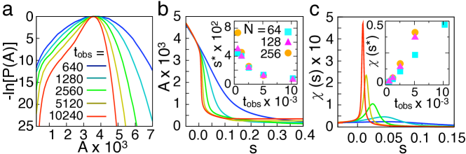
Figure 4: First-order dynamical phase transition in the $s$-ensemble with activity measured in terms of enduring kinks. (a) Probability of observing a trajectory with intensive activity $A$ as a function of $t_{\mathrm{obs}}$ for the $d=1$ East model at $T=0.72$ and $N=64$. (b) $A$ as a function of $s$ for the same systems sampled in (a). The value of $s^{*}$ is plotted as a function of $t_{\mathrm{obs}}$ in the inset for different system sizes $N$. (c) Susceptibility $\chi(s)$ as a function of $s$. The inset shows the peak of the susceptibility, $\chi(s^{*})$ as a function of $t_{\mathrm{obs}}$ for different $N$.

References

- Merolle et al. (2005) M. Merolle, J. Garrahan, and D. Chandler, Proc. Natl. Acad. Sci. USA 102, 10837 (2005).
- Garrahan et al. (2007) J. P. Garrahan, R. L. Jack, V. Lecomte, E. Pitard, K. van Duijvendijk, and F. van Wijland, Phys. Rev. Lett. 98, 195702 (2007).
- Hedges et al. (2009) L. O. Hedges, R. L. Jack, J. P. Garrahan, and D. Chandler, Science 323, 1309 (2009).
- Speck and Chandler (2012) T. Speck and D. Chandler, J. Chem. Phys. 136, 184509 (2012).
- Speck et al. (2012) T. Speck, A. Malins, and C. P. Royall, Phys. Rev. Lett. 109, 195703 (2012).
- Jack et al. (2011) R. L. Jack, L. O. Hedges, J. P. Garrahan, and D. Chandler, Phys. Rev. Lett. 107, 275702 (2011).
- (7) For general reviews on the glass transition problem and on different theoretical approaches see, e.g., M. Ediger, C. Angell, and S. Nagel, J. Phys. Chem. 100, 13200 (1996); V. Lubchenko and P. G. Wolynes, Annu. Rev. Phys. Chem. 58, 235 (2007); A. Cavagna, Phys. Rep. 476, 51 (2009); D. Chandler and J. P. Garrahan, Annu. Rev. Phys. Chem. 61, 191 (2010); K. Binder and W. Kob, Glassy materials and disordered solids (World Scientific, 2011); L. Berthier and G. Biroli, Rev. Mod. Phys. 83, 587 (2011); G. Biroli and J.P. Garrahan, J. Chem. Phys. 138, 12A301 (2013).
- Keys et al. (2011) A. S. Keys, L. O. Hedges, J. P. Garrahan, S. C. Glotzer, and D. Chandler, Phys. Rev. X 1 (2011).
- Garrahan and Chandler (2003) J. P. Garrahan and D. Chandler, Proc. Natl. Acad. Sci. 100, 9710 (2003).
- Elmatad et al. (2009) Y. S. Elmatad, D. Chandler, and J. P. Garrahan, J. Phys. Chem. B 113, 5563 (2009).
- Elmatad et al. (2010) Y. S. Elmatad, D. Chandler, and J. P. Garrahan, J. Phys. Chem. B 114, 17113 (2010).
- Note (1) is the crossover temperature below which dynamics is spatially heterogeneous. Below that temperature, the structural relaxation time is super-Arrhenius, obeying the parabolic law Garrahan and Chandler (2003); Elmatad et al. (2009), and above that temperature, the structural relaxation time is Arrhenius or sub-Arrhenius. Reversible transport properties at very low temperatures can be predicted quantitatively by extrapolation from behavior near but below Keys et al. (2011); Elmatad et al. (2010). Thus, we see is no evidence for another dynamical crossover in reversible supercooled glass forming liquids.
- Stillinger and Weber (1982) F. H. Stillinger and T. A. Weber, Phys. Rev. A 25, 978 (1982).
- Widmer-Cooper et al. (2004) A. Widmer-Cooper, P. Harrowell, and H. Fynewever, Phys. Rev. Lett. 93, 135701 (2004).
- Note (2) Ref. Widmer-Cooper et al. (2004) considered iso-configurational averaging with rather than with . In that case, vibrations obscure structure, especially for short trajectories. Burnishing with , not , produces a vivid picture.
- Manning and Liu (2011) M. L. Manning and A. J. Liu, Phys. Rev. Lett. 107, 108302 (2011).
- Garrahan and Chandler (2002) J. P. Garrahan and D. Chandler, Phys. Rev. Lett. 89, 35704 (2002).
- Palmer et al. (1984) R. G. Palmer, D. L. Stein, E. Abrahams, and P. W. Anderson, Phys. Rev. Lett. 53, 958 (1984).
- Note (3) For , . For dimensions and 3, numerics Keys et al. (2011) finds and 2.4, respectively, and is of order one, with a specific value that is system dependent.
- Keys et al. (2013) A. S. Keys, J. P. Garrahan, and D. Chandler, Proc. Natl. Acad. Sci. USA 110, 4482 (2013).
- Hedges et al. (2007) L. O. Hedges, L. Maibaum, D. Chandler, and J. P. Garrahan, J. Chem. Phys. 127, 211101 (2007).
- Lecomte et al. (2007) V. Lecomte, C. Appert-Rolland, and F. van Wijland, J. Stat. Phys. 127, 51 (2007).
- Note (4) There is significant freedom in the specific choice of dynamical activity. For example, a suitable alternative Speck and Chandler (2012) is , where is a particle diameter or a fraction of a particle diameter, is the unit Heaviside function, the sum on is over all particles, and the sum on is over time intervals of width extending from 0 to .
- Limmer and Chandler (2013) D. Limmer and D. Chandler, arXiv:1306.4728 (2013).
- Jäckle and Eisinger (1991) J. Jäckle and S. Eisinger, Z. Phys. B 84, 115 (1991).
- Elmatad and Keys (2012) Y. S. Elmatad and A. S. Keys, Phys. Rev. E 85, 061502 (2012).
- Sollich and Evans (2003) P. Sollich and M. R. Evans, Phys. Rev. E 68, 031504 (2003).
- Ashton et al. (2005) D. J. Ashton, L. O. Hedges, and J. P. Garrahan, J. Stat. Mech. Theor. Exp. 2005, P12010 (2005).
- Aldous and Diaconis (2002) D. Aldous and P. Diaconis, J. Stat. Phys. 107, 945 (2002).
- Chleboun et al. (2013) P. Chleboun, A. Faggionato, and F. Martinelli, J. of Stat. Mech. Theor. Exp. 2013, L04001 (2013).
- Note (5) When is short compared to (i.e., the regime most relevant for aging protocols) Sollich and Evans (1999). For longer , is reduced by entropic effects to a limiting value Chleboun et al. (2013).
- Sollich and Evans (1999) P. Sollich and M. R. Evans, Phys. Rev. Lett. 83, 3238 (1999).
- Bodineau et al. (2012) T. Bodineau, V. Lecomte, and C. Toninelli, J. Stat. Phys. 147, 1 (2012).
- Jack et al. (2006) R. L. Jack, J. P. Garrahan, and D. Chandler, J. Chem. Phys. 125, 184509 (2006).
- Torrie and Valleau (1977) G. M. Torrie and J. P. Valleau, J. Comp. Phys. 23, 187 (1977).
- Shirts and Chodera (2008) M. R. Shirts and J. D. Chodera, J. Chem. Phys. 129 (2008).