Characteristic functions Describing the Power Absorption Response of Periodic Structures to Partially Coherent Fields

Abstract

Many new types of sensing or imaging surfaces are based on periodic thin films. It is explained how the response of those surfaces to partially coherent fields can be fully characterized by a set of functions in the wavenumber spectrum domain. The theory is developed here for the case of 2D absorbers with TE illumination and arbitrary material properties in the plane of the problem, except for the resistivity which is assumed isotropic. Sum and differerence coordinates in both spatial and spectral domains are conveniently used to represent the characteristic functions, which are specialized here to the case of periodic structures. Those functions can be either computed or obtained experimentally. Simulations rely on solvers based on periodic-boundary conditions, while experiments correspond to Energy Absorption Interferometry (EAI), already described in the literature. We derive rules for the convergence of the representation versus the number of characteristic functions used, as well as for the sampling to be considered in EAI experiments. Numerical examples are given for the case of absorbing strips printed on a semi-infinite substrate.

I Introduction

Periodic absorbing structures are ubiquitous in detector systems at sub-mm and far-infrared wavelengths. At the lowest level, the thin-film absorbers of individual bolometric detectors may be patterned on sub-wavelength scales to realise a frequency selective surface perera2006optical , or to allow the removal of substrate heat capacity while still matching the impedance of the film to free space mauskopf1997composite . At the highest level, an imaging array of such detectors can itself be modelled as a periodic absorbing surface. Periodic structures may also be used for wavelength filtering bossard2006design . The radiation of interest at these wavelengths is often thermal in origin, for example in passive imaging for astronomy, earth observation and security screening. In this case the radiation can no longer be assumed spatially coherent over the whole of the absorbing surface, as it arises from a collection of incoherent emitters. An understanding of how partially coherent fields interact with periodic surfaces is therefore critical to understanding and optimizing the behaviour of these systems.

This paper provides a framework for the characterisation of the absorption response of such periodic surfaces to fields in any state of spatial coherence. The correlation between fields will be written with the help of a finite series of eigenfunctions $\phi_{n}$, as described in man95 . Powers absorbed for each of those eigenfunctions will then simply add up. For general surfaces, those powers will be written in wavenumber spectral domain as a reaction between field eigenfunctions and a cross-spectral power density $P^{\circ}$. Sum and difference coordinates will be used in both spatial and spectral domains. For periodic surfaces $P^{\circ}$ will be shown to be a discrete spectrum (numbered with index $v$) versus spectral difference coordinates, while its dependence on spectral sum coordinates is fully described by a set of characteristic functions ${\cal H}_{v}$.

Those characteristic functions can be obtained either through measurement or simulation. An appropriate measurement technique is Energy Absorption Interferometry (EAI), first mentioned in sak07 and wit07 , simulated in in tho10 and put in practice tho12 . Briefly, a pair of sources is used to illuminate the surface and the absorbed power is recorded as the relative phase between sources is rotated. We explain how the correlation functions $C_{12}$ obtained from those experiments can be exploited to compute characteristic functions ${\cal H}_{v}$. This theory may be viewed as an extension of sak07 in the following respects: $(i)$ introduction of the evanescent part of the spectrum, such that near-field sources or scatterers can be included in the analysis, $(ii)$ use of sum-and-difference spectral coordinates, $(iii)$ precise link with EAI data and $(iv)$ specialization to periodic structures, while general surfaces as well as laterally homogeneous surfaces will also be treated. Numerical examples will be given for the simple case of strips printed onto a semi-infinite medium. The numerical simulation of EAI experiments involves the response of the periodic structure to a single source; as introduced in wit11 , such a response can be obtained from the periodic-source case with the help of the Array Scanning Method (ASM, mun79 ). A phasor notation will be used throughout the paper, with an $\exp(j\,\omega\,t)$ time dependence (with $\omega$ radian frequency and $\sqrt{-1}=j$) suppressed.

The remainder of this paper is organized as follows. Section 2 provides a general spectral-domain representation of power absorbed by an arbritrary surface. Section 3 specializes that result to 1D-periodic surfaces through the definitions of characteristic functions ${\cal H}_{v}$ of spectral sum coordinates. Section 4 explains how the cross-spectral power density $P^{\circ}$ can be obtained from EAI experiments over arbitrary surfaces, while Section 5 specializes this result for periodic structures and provides a simple rule regarding the convergence of the proposed representation versus number of characteristic functions. Section 6 makes use of the ASM to explain how the characteristic functions can be obtained with periodic boundary condition solvers. Section 7 summarizes the results for the special case of laterally invariant surfaces (but still arbitrary versus depth). Section 8 provides numerical results for periodic surfaces made of strips printed on a semi-infinite medium. A summary and conclusions are provided in Section 9. To ease the reading of the paper, the main quantities defined in this paper are summarized in Appendix B.

II Power absorbed by an arbitrary 2D surface

In this section, we provide a general expression for the power absorbed by a 2D semi-infinite absorber, based on the response of the absorber in terms of induced conduction currents (see sketch in Fig. 1). The excitations correspond to incident plane waves, which can be either propagating or evanescent. The result makes use of previously published coherent-mode representations of partially-coherent fields man95 .

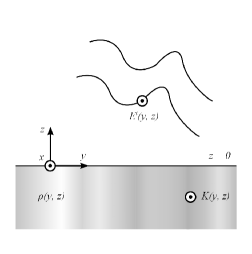
Figure 1: Partially coherent field incident on arbitrary semi-infinite medium, leading to induced current density $K(x,y)$.

The absorbing material occupies a semi-infinite space defined by $z<0$ and is invariant along $x$. It is characterized by its real permittivity, its equivalent conductivity (including effect of dielectric losses) and its real permeability, with arbitrary dependence on $y$ and $z$ coordinates. The inverse of the equivalent conductivity will be denoted by $\rho(y,z)$ and the induced conduction current density by $K(y,z)$. Incident fields are assumed to have TE polarization; the extension to TM polarization should be straightforward. Likewise, the extensions to doubly periodic structures and to anisotropic resistivity should be straightforward as well.

Let us denote by $E^{i}(y)$ the incident field at the $z=0$ level; it can be expressed in spectral domain as $\tilde{E}^{i}(k_{y})$:

$$E^{i}(y)=\frac{1}{2\,\pi}\ \int_{-\infty}^{\infty}\,\tilde{E}^{i}(k_{y})\,\exp(-j\,k_{y}\,y)\,dk_{y}.$$ (1)

The current density induced by the field in the absorber may then be expressed in the form:

$$K(y,z)=\frac{1}{2\,\pi}\ \int_{-\infty}^{\infty}\,\tilde{E}^{i}(k_{y})\,K^{\circ}(y,z|k_{y})\,dk_{y}$$ (2)

where $K^{\circ}(y,z|k_{y})$ is the current density in response to a unit-magnitude incident field at the $z=0$ level, with $\exp(-j\,k_{y}\,y)$ horizontal dependence. The expectance value for absorbed power per unit length along $x$ is:

$$P=\frac{1}{2}\,\int_{-\infty}^{0}\,\int_{-\infty}^{\infty}\,\rho(y,z)\,\left\langle|K(y,z)|^{2}\right\rangle\,dy\,dz$$ (3)

where angle brackets denote ensemble average. Using (1) and (2), the power can be rewritten as

$$P=\frac{1}{2}\,\frac{1}{(2\,\pi)^{2}}\,\int_{k_{y1}}\int_{k_{y2}}\ \tilde{\mathcal{E}}^{i}(k_{y1},k_{y2})\,P^{\circ}(k_{y1},k_{y2})\,dk_{y1}\,dk_{y2}$$ (4)

where

$$\tilde{\mathcal{E}}^{i}(k_{y1},k_{y2})=\langle\tilde{E}^{i}(k_{y1})\tilde{E}^{i,\star}(k_{y2})\rangle$$ (5)

is the spectral cross-correlation function of the incident field and

$$P^{\circ}(k_{y1},k_{y2})=\int_{S}\,\rho\,K^{\circ}(y,z|k_{y1})\,K^{\circ,\star}(y,z|k_{y2})\,dS$$ (6)

where S refers to the half space $z<0$. $P^{\circ}$ is a response function that fully characterises the absorption behaviour of the surface. Hereafter $P^{\circ}$ will be named the cross-spectral power density. Here “spectral” refers to the spatial wavenumber spectrum and “cross-spectral” refers to the fact that it depends on two spectral coordinates. In the above expressions, the angle brackets denote ensemble averages. We have assumed that the field is a stationary random process, such that the different frequency components are incoherent.

Equation (4) shows that the absorbed power is a function of the second-order spatial correlations in the incident field, as characterised by $\tilde{\mathcal{E}}^{i}(k_{y1},k_{y2})$. In the case of a Gaussian random field (as is the case for most thermal fields), knowledge of the second-order correlation function allows all higher-order moments to be calculated man95 . A conceptually appealing representation of a partially-coherent field is given in terms of its coherent modes wol86 . These form a set of functions $\tilde{\phi}_{i}(k_{y})$ that diagonalise the correlation function,

$$\tilde{\mathcal{E}}^{i}(k_{y1},k_{y2})=\sum_{n}\gamma_{n}\tilde{\phi}_{n}(k_{y1})\tilde{\phi}^{\star}_{n}(k_{y2}),$$ (7)

so that partial coherence in the field can be thought of as arising from mutually incoherent superposition of these individually fully coherent fields. Substituting this representation into (4) we obtain the result

$$P = \frac{1}{8\,\pi^{2}}\,\sum_{n}\,\gamma_{n}\,\int_{k_{y1}}\int_{k_{y2}}\ \tilde{\phi}_{n}(k_{y1})\,P^{\circ}(k_{y1},k_{y2})$$ (8)

$$\hskip 113.81102pt\tilde{\phi}_{n}^{\star}(k_{y2})dk_{y1}\,dk_{y2},$$

use of which will be made later.

This formulation may be viewed as an extension of equation (56) of sak07 to the evanescent part of the spectrum, which allows the analysis of the response of the sensor to near-field sources. Contrary to (56) of sak07 , the analysis presented here is kept in frequency domain.

III Power absorbed by a periodic 2D surface

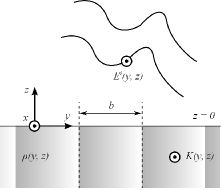
Figure 2: Partially coherent field incident on semi-infinite medium with period $b$ along $y$ coordinate.

Let us now assume that the absorbing structure is periodic with period $b$ along $y$, while the structure of the incident wave remains entirely arbitrary (see sketch in Fig. 2). The integrand appearing in the expression, (6), for the cross-spectral power density involves three factors. The first one, the resistivity $\rho(y,z)$, is periodic versus $y$ with period $b$, while the second and third ones, current densities $K^{\circ}(y,z|k_{y1})$ and $K^{\circ,\star}(y,z|k_{y2})$, are also periodic with same period but with linear phase progressions at rates $k_{y1}$ and $-k_{y2}$, respectively. Hence, the product between those three functions is periodic along $y$ with period $b$, except for a phase progression at rate $k_{y1}-k_{y2}$. Hence, the integrand of (6) corresponds, after multiplication by a phase factor $\exp(j\,(k_{y1}-k_{y2})\,y)$, to a purely periodic function. Therefore, we can write the Fourier series:

$$\rho(y,z)\,K^{\circ}(y,z|k_{y1})\,K^{\circ,\star}(y,z|k_{y2})=$$

$$\hskip 5.69046pt\frac{1}{2\pi}e^{-j\,(k_{y1}-k_{y2})\,y}\,\sum_{v=-\infty}^{\infty}\,{Q}_{v}(z|k_{y1},k_{y2})\,e^{j\,v\,y\,2\pi/b}$$ (9)

with

$${Q}_{v}(z|k_{y1},k_{y2})=$$

$$\frac{2\,\pi}{b}\ \int_{0}^{b}\rho(y,z)\,K^{\circ}(y,z|k_{y1})\,K^{\circ,\star}(y,z|k_{y2})\,$$

$$e^{j\,(k_{y1}-k_{y2})\,y}\,e^{-j\,v\,y\,2\pi/b}\ dy.$$ (10)

Then, introducing that Fourier series into (6), rearranging the order of integrations along $y$ and noting that $\int_{-\infty}^{\infty}\,\exp(j\,\zeta)\,d\zeta=2\pi\,\delta(\zeta)$, we obtain:

$$P^{\circ}(k_{y1},k_{y2})=\sum_{v=-\infty}^{\infty}\,{\cal H}_{v}(k^{+})\,\delta(k^{-}-v\,\frac{2\pi}{b})$$ (11)

with the following definitions of sum and difference wavenumbers:

$$k^{+}=(k_{y1}+k_{y2})/2\ \ \ \ \mbox{and}\ \ \ \ k^{-}=k_{y1}-k_{y2}$$ (12)

and the following characteristic function

$${\cal H}_{v}(k^{+}) = \frac{2\pi}{b}\,\int_{S_{\circ}}\,\rho\,K^{\circ}\left(y,z|k^{+}+v\,\frac{\pi}{b}\right)$$ (13)

$$K^{\circ,\star}\left(y,z|k^{+}-v\,\frac{\pi}{b}\right)\,dS_{\circ}$$

where $S_{o}$ is the unit cell of the periodic structure ($0\leq y<b$). We have also used the $k^{-}=2\pi v/b$ determination imposed by the presence of the delta function to write $k_{y1}$ and $k_{y2}$ in terms of $k^{+}$. The induced currrent density $K^{\circ}$ over the unit cell, and hence also the characteristic functions ${\cal H}_{v}$ can be computed with any type of periodic boundary conditions solver. The structure of the cross-spectral power density $P^{\circ}$ is sketched in Fig. 3.

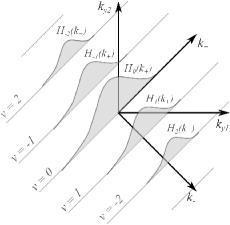
Figure 3: Structure of cross-spectral power density in sum-and-difference spectral coordinates: discrete spectrum characterized by ${\cal H}_{v}(k^{+})$ functions.

Inserting (11) into (8), the definition of the characteristic function ${\cal H}_{v}(k^{+})$ yields the following general expression for the power absorbed into periodic structures of period $b$:

$$P = \frac{1}{8\,\pi^{2}}\,\sum_{n}\,\gamma_{n}\,\sum_{v=-\infty}^{\infty}\,\int_{k^{+}}\,\tilde{\phi}_{n}\left(k^{+}+v\,\frac{\pi}{b}\right)$$ (14)

$$\hskip 56.9055pt\tilde{\phi}_{n}^{\star}\left(k^{+}-v\,\frac{\pi}{b}\right)\,\,{\cal H}_{v}(k^{+})\,dk^{+}.$$

In the following two sections, we propose a methodology for obtaining the ${\cal H}_{v}$ functions from data obtained through an interferometric measurement technique.

IV Characterization through Energy Absorption Interferometry

Figure 4: Basic operating principle of Energy Absoption Interferometry.

Energy Absorption Interferometry (EAI) is a technique that was originally proposed for detector characterisation wit07 , and has recently been demonstrated experimentally in this context tho12 . More recently, its use as a general tool for characterising power absorption in structures has been studied with12 . As illustrated in Fig. 4, EAI involves illuminating the Structure Under Test (SUT) with a pair of phase-locked sources and recording the power absorbed. As the relative phase between two sources is rotated, the detector output displays a fringe pattern, the complex amplitude of which characterises the detector response. This section explains how the response function $P^{\circ}$ defined in (6) can be measured from this fringe amplitude, allowing the calculation of absorbed power for any incident field. This will be done first for arbitrary (i.e. non-periodic) absorbers.

In the 2D case treated here the sources are infinite line sources oriented along $x$ and of intensity $I$. The dissipated power can be written as:

$$P^{l}=\frac{1}{2}\,\int\,\rho\,|K^{l}|^{2}\ dS$$ (15)

where $K^{l}$ corresponds to the current density excited by a line source of intensity $I$ located a height $z=h$ and horizontal coordinate $y=y_{s}$. Superscript $l$ reminds us that the absorbed power has been obtained with the line-source illumination in an EAI experiment.

It is easy to prove that, for two sources, with intensities $I_{1}=I$ and $I_{2}=I\,e^{j\,\phi}$, located at $(y_{s}=y_{1},h)$ and $(y_{s}=y_{2},h)$ respectively, we have:

$$P^{l}(y_{1},y_{2})=\frac{1}{2}\,\left(\alpha_{11}+\alpha_{22}+2\,\alpha_{12}\,\cos(\phi-\beta_{12})\right)$$ (16)

with correlation functions defined as:

$$C_{ij}(y_{1},y_{2}) = \alpha_{ij}\,e^{j\,\beta_{ij}}$$ (17)

$$= \!\!\!\int_{-\infty}^{0}\!\!\int_{-\infty}^{\infty}\!\!\rho\,K^{l}_{i}(y,z)K_{j}^{l,\star}(y,z)\,dydz$$ (18)

$$= \int\,\rho\,K_{i}^{l}\,K_{j}^{l,\star}\ dS$$ (19)

where $K^{l}_{i}$ is the current density induced by the line source located at $y=y_{si}$. Combining experimental results with one and two sources, the correlation function $C_{12}$ is readily obtained. The remainder of this section consists of providing a link between that correlation function and the cross-spectral power density $P^{\circ}(k_{y1},k_{y2})$, defined in (6) and that completely characterizes the absorber.

We start with the current induced in the absorber when only one line source is present, with current $I$ and position $(y,z)=(y_{s},h)$. The incident field at $z=0$ from the current source is decomposed into plane waves as (mor53 , Sec. 7.3):

$$E^{i}(y)=-\frac{I\,k\,\eta}{2\,\pi}\,\int_{-\infty}^{\infty}\,\frac{e^{-j\,k_{y}\,(y-y_{s})}e^{-jk_{z}h}}{2\,k_{z}}\,dk_{y}$$ (20)

with the following constraint:

$$k_{y}^{2}+k_{z}^{2}=k^{2}=\omega^{2}/c^{2}$$ (21)

where $\omega$ is the radian frequency and $c$ is the speed of light in free space. The corresponding induced current density $K^{l}$ is obtained by simply introducing in the integrand the current density $K^{\circ}(y,z|k_{y})$ obtained with a unit-magnitude incident electric field with $e^{-j\,k_{y}\,y}$ dependence:

$$K^{l}_{i}(y,z)=-\frac{I\,k\,\eta}{2\,\pi}\ \int_{-\infty}^{\infty}\,K^{\circ}(y,z|k_{y})\,\frac{e^{j\,k_{y}\,y_{s,i}}e^{-jk_{z}h}}{2\,k_{z}}\ dk_{y}.$$ (22)

From this plane-wave decomposition, the correlation (19) can be linked with the cross-spectral power density $P^{\circ}$ defined in (6):

$$C_{12}(y_{1},y_{2}) = \frac{k^{2}\,\eta^{2}\,|I|^{2}}{4\,(2\,\pi)^{2}}\,\int_{k_{y1}}\!\!\int_{k_{y2}}\,P^{\circ}(k_{y1},k_{y2})$$ (23)

$$\frac{e^{j\,(k_{y1}\,y_{1}-k_{y2}\,y_{2})}\,e^{-j\,(k_{z1}\pm k_{z2})\,h}}{k_{z1}\,k^{\star}_{z2}}\,dk_{y1}\,dk_{y2}$$

where the $+$ sign is taken when $k_{z2}$ becomes imaginary. Since it will be interesting to see to what extent correlations depend on average positions, besides dependence on difference between coordinates. To clarify this, we make the following sum-and-difference change of variables:

$$r=(y_{1}+y_{2})/2,\ \ \ \ \ \ s=y_{1}-y_{2}$$ (24)

Together with (12) this allows us to rewrite the correlation as:

$$C_{12}(y_{1},y_{2}) = \frac{k^{2}\,\eta^{2}\,|I|^{2}}{4\,(2\,\pi)^{2}}\,\int_{k^{+}}\!\!\int_{k^{-}}\,P^{\circ}(k_{y1},k_{y2})\,$$ (25)

$$\frac{e^{j\,(k^{+}\,s+k^{-}\,r)}\,e^{-j\,(k_{z1}\pm k_{z2})\,h}}{k_{z1}\,k^{\star}_{z2}}\,dk^{+}\,dk^{-}$$

where $(k_{y1},k_{y2})$ wavenumbers (and related $(k_{z1},k_{z2})$ quantities, see (21)) can be readily obtained from the definitions (12) of $k^{+}$ and $k^{-}$. It is important to notice that equation (25) has the form of a 2D Fourier transform. This observation leads us to the fact that the cross-spectral power density $P^{\circ}(k_{y1},k_{y2})$ can be obtained through inverse Fourier transformation:

$$P^{\circ}(k_{y1},k_{y2}) = \frac{4\,k_{z1}\,k_{z2}^{\star}}{k^{2}\,\eta^{2}\,|I|^{2}}\,e^{j\,(k_{z1}\pm k_{z2})\,h}$$ (26)

$$\int_{r}\,\int_{s}\ C_{12}(r,s)\ e^{-j\,(k^{+}\,s+k^{-}\,r)}\ dr\,ds$$

where sum and difference coordinates have been used in both spatial and spectral domains. Regarding the latter, in order to simplify the notation, we have mixed $(k_{y1},k_{y_{2}})$ coordinates (and related $(k_{z1},k_{z_{2}})$ wavenumbers) with $(k^{+},k^{-})$ coordinates, with the link between variables given by (12).

V Characterization of a periodic 2D absorber

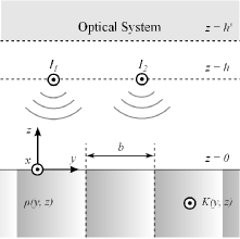
Figure 5: Energy Absorption Interferometry above a periodic surface.

In this section, the periodicity of the structure is introduced by noticing that the correlation function is periodic versus the sum coordinate $r=(y_{1}+y_{2})/2$. A Fourier series representation of the correlation function obtained from EAI (Fig. 5) leads to a discrete-spectrum representation of the cross-spectral power density and, in turn, to a combined discrete and continuous spectral representation of the absorbed power. A direct link is established between correlation functions and characteristic functions ${\cal H}_{v}$ describing the periodic absorber.

If $y_{1}$ and $y_{2}$ are the positions of the sources, we may represent the correlations in the $RS$ plane, defined through (24). In view of the periodicity of the absorber, we may expect the correlation function to be periodic of period $b$ versus sum coordinate $r$. This allows us to write the dependence of $C_{12}$ as a Fourier series along $r$, in which each term is a function of $s$:

$$C_{12}(y_{1},y_{2})=C_{12}(r,s)=\frac{1}{2\,\pi}\,\sum_{v=-\infty}^{\infty}\,e^{j\,\frac{2\,\pi}{b}\,v\,r}\,H_{v}(s).$$ (27)

The $H_{v}$ functions can be obtained from the correlation data as:

$$H_{v}(s)=\frac{2\,\pi}{b}\,\int_{0}^{b}\,C_{12}(r,s)\,e^{-j\,\frac{2\,\pi}{b}\,v\,r}\ dr.$$ (28)

The cross-spectral power density (26) can then be re-written for the specific case of periodic absorbers via the following observation:

$$\int_{r}\,\int_{s}\ C_{12}(r,s)\ e^{-j\,(k^{+}\,s+k^{-}\,r)}\ dr\,ds=$$

$$\frac{1}{2\,\pi}\,\sum_{v}\,\int_{s}\,H_{v}(s)\,e^{-j\,k^{+}\,s}\int_{r}\,e^{j\,v\,\frac{2\,\pi}{b}\,r}\,e^{-j\,k^{-}\,r}\ dr\,ds$$ (29)

where the integral over $r$ produces $2\,\pi\,\delta\left(k^{-}-v\,{2\,\pi}/{b}\right)$. From there, the following result is obtained for the cross-spectral power density (26):

$$P^{\circ}(k_{y1},k_{y2}) = \frac{4\,k_{z1}\,k_{z2}^{\star}}{k^{2}\,\eta^{2}\,|I|^{2}}\,e^{j\,(k_{z1}\pm k_{z2})\,h}\,$$ (30)

$$\sum_{v}\int_{s}\ H_{v}(s)\ e^{-j\,k^{+}\,s}\,ds\ \delta\left(k^{-}-v\,\frac{2\,\pi}{b}\right)$$

This result allows us to write the absorbed power (8) for arbitrary partially-coherent incident fields as:

$$P = \frac{1}{2\,\pi^{2}}\,\frac{1}{k^{2}\,\eta^{2}\,|I|^{2}}\,\sum_{n}\gamma_{n}\sum_{v}\int_{k^{+}}\,k_{z1}\,k_{z2}^{\star}\,$$ (31)

$$e^{j\,(k_{z1}\pm k_{z2})\,h}\,\tilde{\phi}_{n}(k_{y1})\,\tilde{\phi}_{n}^{\star}(k_{y2})$$

$$\int_{s}\ H_{v}(s)\ e^{-j\,k^{+}\,s}\,ds\ dk^{+}$$

where, as a result of (12) and of the presence of a Dirac delta function in (30), we have

$$k_{y1}=k^{+}+v\,\pi/b\ \ \ \ \ \mbox{and}\ \ \ \ \ k_{y2}=k^{+}-v\,\pi/b.$$ (32)

To ease further interpretation, in a different notation, the absorbed power reads:

$$P = M_{0}\ \sum_{n}\gamma_{n}\sum_{v}\int_{-\infty}^{\infty}\,k_{z1}\,k_{z2}^{\star}\,$$ (33)

$$e^{j\,(k_{z1}\pm k_{z2})\,h}\,\tilde{\phi}_{n}(k_{y1})\,\tilde{\phi}_{n}^{\star}(k_{y2})\,\tilde{H}_{v}(k^{+})\,dk^{+}$$

where $M_{0}=1/2\,\left(\pi\,k\,\eta|I|\right)^{-2}$ and $\tilde{H}_{v}(k^{+})$ is the Fourier transform of $H_{v}(s)$. For $v=0$, the interpretation is very simple: for each coherent eigenfield $\phi_{i}$, the absorbed power is proportional to an inner product between the spectral density $|\tilde{\phi}_{i}|^{2}$ of the incident field and the sensitivity $\tilde{H}_{0}$, given as the Fourier transform of the average correlation (averaging over absolute coordinates $r$ along unit cell $b$, within a factor $2\,\pi$) obtained from the EAI experiments. For $v\not=0$, the interpretation is more complex, the spectral density is replaced by the $\tilde{\phi}_{i}(k_{y1})\,\tilde{\phi}_{i}^{\star}(k_{y2})$ product and the sensitivity is replaced by the Fourier transform of the $H_{v}(s)$ function, corresponding to a non-fundamental component of the periodic (versus $r$) correlation function.

From the expression (33) of absorbed power, it is now clear that the function $\exp({j\,(k_{z1}\pm k_{z2})\,h})\,\tilde{H}_{v}(k^{+})$ completely defines the power response of the periodic structure. The function $\tilde{H}_{v}(k^{+})$ depends on the height at which the EAI experiments have been carried out and the $\exp({j\,(k_{z1}\pm k_{z2})\,h})$ factor propagates those results to zero height. Comparing forms (14) and (33) of absorbed power, one obtains the following link between characteristic functions of the absorber and Fourier transform of correlation functions obtained from EAI experiments:

$${\cal H}_{v}(k^{+})=e^{j\,(k_{z1}\pm k_{z2})\,h}\,\tilde{H}_{v}(k^{+})\frac{4\,k_{z1}\,k_{z2}^{\star}}{k^{2}\,\eta^{2}\,|I|^{2}}.$$ (34)

The minus sign before $k_{z2}$ has to be used when $|k^{+}-v\,\pi/b|>k$ (upward evanescent wave). We here recall the link (21) between $k_{z}$ and $k_{y}$ and the link (32) between $k_{y}$ and $k^{+}$ and $v$. Those relations will be important for the understanding of the following.

One may wonder about the importance of integrating (14) outside the visible region, i.e. for $|k^{+}|>k$, where evanescent waves are involved. It is well known that energy transfer can actually take place via evanescent waves, provided that there are transmitted and reflected waves. Those evanescent waves may be radiated by the observed object located in the near field or may be scattered by parts of the observation instrument. Let us denote by $h^{s}$ the lowest parts of the observed sources or of the instrument (see Fig. 5). That height corresponds to the characteristic distance over which evanescent waves may propagate toward the surface; evanescent waves propagating over longer distances will simply undergo stronger decay. When either $k_{y1}$ or $k_{y2}$, as given by (32), lies outside the visible region ($|k_{y}|>k$), the function $F=\tilde{\phi}_{n}(k_{y1})\,\tilde{\phi}_{n}^{\star}(k_{y2})$ decays by a factor $|\exp({-j\,(k_{z1}\pm k_{z2})\,h^{s}})|$ wol86 . In the expression (14) for the absorbed power, that decay combines with the exponential factor appearing in the expression of ${\cal H}_{v}(k^{+})$, given in (34). This leads to a decay ($D>1$) in total power given by:

$$D=|e^{{-j\,(k_{z1}\pm k_{z2})\,(h^{s}-h)}}|$$ (35)

where $k_{z1}$ or $k_{z2}$ (or both) can be imaginary, thus leading to exponential decay.

The convergence of the proposed representation versus index $v$ can be estimated in the limit of large $v$. We estimate here a lower bound for $D$. Wavenumbers $k_{z1}$ and $k_{z2}$ are linked to $k_{y1}$ and $k_{y2}$ through (21). We also know that $k_{y1}-k_{y2}=v\,2\pi/b$, through (32). The slowest decay rate will be obtained when one of the wavenumbers, say $k_{y2}$, lies within the visible region, which imposes $|k_{y2}|<k$. For large values of $v$, such that $v\,2\pi/b\gg k$, we obtain $k_{z1}\simeq-j\,v\,2\pi/b$ (from (21) for large $k_{y}$). This leads to a very simple model for the slowest decay versus index $v$:

$$D\simeq e^{|v|\,\frac{2\,\pi}{b}\,(h-h_{s})}$$ (36)

which, in dB scale, corresponds to a decay by a factor

$$D_{dB}\simeq\frac{20\,\pi}{\ln 10}\,\frac{h_{s}-h}{b}\,|v|.$$ (37)

This simple model does not account for the link between incident plane waves and induced currents, but this link is material-dependent and there is no a priori known reason for having a strong (e.g. exponential) dependence on $v$ of induced currents. Also, the model proposed above is well supported by the simulation data presented in Section VIII, where that model will be shown to be very accurate.

To avoid ill-posedness in the characterization of the periodic absorber, it makes sense to avoid too high values of $D$, which suggests $h<h^{s}$ as a recommended mode of operation if one wants to include the evanescent part of the spectrum in the analysis. In other words, if the observed sources or parts of the instrument are in the near-field of the detector, it is advised to conduct EAI experiments at even lower height.

The above observations regarding convergence have important implications in terms of spatial sampling rate in the EAI experiments. First, for a given order $v$, function $H_{v}$ should only be estimated if the signal-to-noise ratio exceeds $D_{dB}$, as given in (37). Having determined the maximum value of $|v|=V_{max}$, it is known that the interval $b$ should be sampled with at least $2V_{max}$ points. Given the fast convergence of successive harmonics, it may not be necessary to use many more points: if all harmonics $|v|>V_{max}$ are truly neglible, then $2V_{max}$ points is strictly sufficient.

Also, obviously, in view of the periodicity of the structure, the displacement of one of the sources can be limited to the unit cell. The other source needs to be shifted over a longer range; the precise range depends on the material properties of the absorber and will not be discussed here in detail.

VI Simulation with periodic boundary condition solvers

The numerical simulation of the response of a given periodic absorber in an EAI experiment requires a priori the estimation of the induced current $K^{l}(y,z)$ for one or two line sources placed above the periodic structure. Since the structure is virtually infinite (or at least large compared to the wavelength), such a simulation requires important computational resources. Here, as introduced in wit11 , we will make use of the Array Scanning Method (ASM) mun79 to express the correlation function in terms of results obtained when considering that both absorbers and sources are infinitely periodic, with a linear phase progression in the source fields. The advantage of this new formulation is that it relies on quantities that can be obtained very fast with the help of unit-cell solvers. Those solvers can be based on either differential or integral-equation approaches.

Using the ASM mun79 , the electric current densities $K$ in the periodic material induced by an isolated source at $y=y_{s}$ can be expressed as the superposition of solutions $K^{\infty}$ with periodic line sources:

$$K^{l}(y_{\circ}+n\,b,z)=\frac{1}{2\,\pi}\ \int_{0}^{2\pi}\ K^{\infty}(y_{\circ},z|\psi)_{|y_{s}}\ e^{-j\,n\,\psi}\ d\psi$$ (38)

where $\psi$ is the phase shift between successive unit cells and $y_{\circ}$ is assumed to be always located within the reference unit cell $S_{\circ}$, i.e. $0\leq y_{\circ}<b$. The index $y_{s}$ denotes the position of the line source within the unit cell. To alleviate notations, the index will be omitted below wherever possible. Besides the explanation given in the original publication mun79 , based on the Poisson summation formula, an alternative proof for (38) is given in cra11 . As explained in cap07 , the infinite-array solution $K^{\infty}$ can be written as an infinite spectral summation (Floquet modes) in which each term corresponds to the effect of one plane wave; from there it is easy to show that swapping summation and integration in (38) is equivalent to integration over the whole spectral axis.

This allows a representation of dissipated power for a single source. Denoting the unit cell, i.e. $-\infty<z\leq 0$ and $0\leq y_{\circ}<b$, by $S_{\circ}$ we have:

$$P = \frac{1}{2}\,\sum_{n=-\infty}^{\infty}\,\int_{-\infty}^{0}\,\int_{0}^{b}\,\rho\,|K^{l}(y_{\circ}+n\,b,z)|^{2}\,dy_{\circ}\,dz$$ (40)

$$= \!\frac{1}{2\,(2\,\pi)^{2}}\!\!\sum_{n=-\infty}^{\infty}\int_{S_{\circ}}\rho\,\left|\int_{0}^{2\pi}K^{\infty}(y_{\circ},z|\psi)e^{-j\,n\,\psi}d\psi\right|^{2}$$

$$\hskip 170.71652ptdS_{\circ}$$

$$= \frac{1}{4\,\pi}\,\int_{0}^{2\,\pi}\,\int_{S_{\circ}}\,\rho\,|K^{\infty}(y_{\circ},z|\psi)|^{2}\,dS_{\circ}\,d\psi$$ (41)

where the transition from (40) to (41) is proven in Appendix A.

In order to obtain the power absorbed in the EAI experiment, the above result is extended to the case of two sources at height $h$ with relative phase shift $\psi$:

$$P = \sum_{n=-\infty}^{\infty}\,\frac{1}{2}\ \int_{S_{\circ}}\,\rho\,|K^{l}_{1}(y_{\circ}+n\,b,z)+$$ (43)

$$\hskip 56.9055ptK^{l}_{2}(y_{\circ}+n\,b,z)\,e^{j\,\phi}|^{2}\,dS_{\circ}$$

$$= \frac{1}{4\,\pi}\int_{0}^{2\,\pi}\int_{S_{\circ}}\rho\,|K_{1}^{\infty}(y_{\circ}+n\,b,z|\psi)+$$

$$\hskip 42.67912ptK_{2}^{\infty}(y_{\circ}+n\,b,z|\psi)\,e^{j\,\phi}|^{2}\,dS_{\circ}\,d\psi$$

$$= \frac{1}{2}\,\left(\alpha_{11}+\alpha_{22}+2\,\alpha_{12}\,\cos(\phi-\beta_{12})\right)$$ (44)

with

$$C_{ij} = \alpha_{ij}\,e^{j\,\beta_{ij}}=\frac{1}{2\,\pi}\int_{0}^{2\,\pi}\,\int_{S_{\circ}}\,\rho\,\ K_{i}^{\infty}(y_{\circ},z|\psi)\,$$ (45)

$$\hskip 56.9055ptK_{j}^{\infty,\star}(y_{\circ},z|\psi)\,dS_{\circ}\,d\psi.$$

We can see that the expression (44) has the same form as (16), but that the correlation functions (45) can now be obtained through integration of products of periodic-source currents $K^{\infty}$ over the unit cell $S_{\circ}$. This will make the simulation feasible with limited computational resources, without simulating fields in huge finite structures.

VII Special case of laterally homogeneous surfaces

In case the absorbing material is not periodic but is invariant along $y$, the results provided thus far can be simplified. A summary of those results is given in this section, considering an arbitrary variation of permittivity, permeability and resistivity versus coordinate $z$.

In this case, the cross-spectral power density $P^{\circ}$ contains only the $v=0$ mode:

$$P^{\circ}(k_{y1},k_{y2})={\cal H}_{0}(k^{+})\,\delta(k_{y1}-k_{y2})$$ (46)

with $k^{+}=k_{y1}=k_{y2}$ and

$${\cal H}_{0}(k^{+})=2\pi\,\int_{-\infty}^{0}\,\rho\,|K^{\circ}(z|k^{+})|^{2}\,dz.$$ (47)

The absorbed power in case of partially coherent incident fields then simplifies as:

$$P=\frac{1}{8\,\pi^{2}}\,\sum_{n}\,\gamma_{n}\,\int_{-\infty}^{\infty}\ |\tilde{\phi}_{n}(k^{+})|^{2}\,{\cal H}_{0}(k^{+})\ dk^{+}$$ (48)

Since correlations $C_{12}$ do not depend on absolute coordinate $r$, (26) can be rewritten as

$$P^{\circ}(k_{y1},k_{y2}) = \frac{4\,k_{z1}\,k_{z2}^{\star}}{k^{2}\,\eta^{2}\,|I|^{2}}\,e^{j\,(k_{z1}\pm k_{z2})\,h}$$ (49)

$$\int_{s}\ C_{12}(s)\ e^{-j\,k^{+}\,s}\,ds\ \delta(k_{y1}-k_{y2})$$

and $C_{12}$ has only one Fourier component:

$$C_{12}(s)=H_{0}(s)/(2\pi)$$ (50)

From the above, it is then possible to provide a simple expression for the sole characteristic function:

$${\cal H}_{0}(k^{+})=\frac{8\,\pi\,k_{z1}\,k_{z2}^{\star}}{k^{2}\,\eta^{2}\,|I|^{2}}\,e^{j\,(k_{z1}\pm k_{z2})\,h}\,\tilde{C}_{12}(k^{+})$$ (51)

with

$$\tilde{C}_{12}(k^{+})=\int_{-\infty}^{\infty}\ C_{12}(s)\ e^{-j\,k^{+}\,s}\,ds.$$ (52)

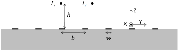
Figure 6: General geometry of simulated structure.

VIII Simulation examples

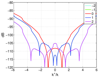
Figure 7: Characteristic functions ${\cal H}_{v}$ for $-2\leq v\leq 2$, for a height of $h=0.25\,\lambda$ from the surface.

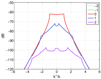
Figure 8: $\tilde{H}_{v}$ functions for a height of $h=0.25\,\lambda$ from the surface.

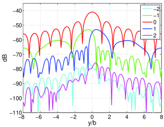
Figure 9: $H_{v}$ functions for a height of $h=0.25\,\lambda$ from the surface.

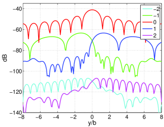
Figure 10: ${H}_{v}$ functions for a height of $0.5\,\lambda$ from the surface.

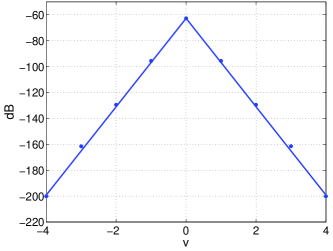
Figure 11: Decay of $H_{v}(0)$ according to simullation (bullets) and according to model (solid), for $h=\lambda/2$.

Simulations have been carried out for the case of an absorber made of a grid of strips placed on a semi-infinite medium (see configuration in Fig. 6). The periodic method of moments har93 cra07 has been used; the Green’s function associated with the semi-infinite medium has been computed in spectral domain tai71 . The free-space wavelength $\lambda$ is 1 mm, the spacing $b$ is 0.4 mm, the width $w$ of the strips is 0.15 mm, the relative permittivity of the medium in the lower half space is $12-j\,0.012$, close to that of undoped silicon, and the sheet impedance of the strips is a tenth of the free-space impedance, i.e. 37.7 Ohm. Four basis functions have been used across the width of each strip. The characteristic functions ${\cal H}_{v}(k^{+})$ will be shown and commented, as well as functions $\tilde{H}_{v}(k^{+})$ and ${H_{v}}(s)$ for two different heights $h$ above the surface.

Fig. 7 shows the magnitudes of ${\cal H}_{v}$ functions for different values of $v$ for a height above the surface equal to $\lambda/4$. It can be seen that $|{\cal H}_{v}|=|{\cal H}_{-v}|$. It is interesting to note that, in the visible region, i.e. for $|k^{+}|<k$, the different functions have the same order of magnitude. Outside the visible region, they tend to grow rapidly. This raises the question of the possible non-bandlimited aspect of those functions. However, one should bear in mind that the absorbed power (14) is computed as a reaction between characterisitic functions ${\cal H}_{v}$ and Fourier transforms of eigenfields $\phi_{n}$ estimated at two different wavenumbers. For large values of the wavenumber $k^{+}$, eigenfields are evanescent and hence can compensate the growth of the ${\cal H}_{v}$ functions. More precisely, if the minimum height of the source or instrument is $h_{s}$, the product $\phi_{n}()\,\phi_{n}^{\star}()$ entails a factor $\exp(j\,(k_{z1}\pm k_{z2})\,h_{s})$. In this expression, $k_{z1}$ and $k_{z2}$ become imaginary outside the visible region, which leads to exponential decay.

For a similar reason, the functions ${\tilde{H}}_{v}(k^{+})$ also decay for large values of $k^{+}$, with a rate proportional to the height $h$ at which EAI experiments have been carried out. Indeed, the (continuous spectrum of) plane waves radiated by the line sources are evanescent for large wavenumbers and hence contribute little to the absorbed power. This effect is visible in Fig. 8, where the ${\tilde{H}}_{v}(k^{+})$ functions are shown. This is also evidenced by the link (34) between characteristic functions ${\cal H}_{v}$ and ${\tilde{H}}_{v}$ functions obtained from correlation measurements. Also, as explained in Section V, the significance of ${\cal H}_{v}$ rapidly decreases as $|v|$ increases. The inverse Fourier transforms of those functions, linked to the EAI experiments according to (28), are shown in Fig. 9. Here too, it can be seen that the significance of those functions decays with $|v|$ and $h$. This can be observed from Fig. 10, where ${\tilde{H}}_{v}$ functions are shown for a larger distance, $h=\lambda/2$. It can be seen from Figs. 9 and 10 that the spatial bandwidth of ${H}_{v}$ functions increases with $|v|$, as confirmed by their Fourier transforms, visible in Fig. 8 for $h=0.25\,\lambda$.

Finally, the decay of functions $H_{v}$ versus $v$ is made explicit for $h=0.5\lambda$ in Fig. 11, where the stars correspond to the result obtained numerically, while the solid line coresponds to the model (37). Since only the decay rate is analyzed here, the value of the model has been arbitrarily set to the numerically obtained value for $v=0$. Excellent agreement is observed between modeled and numerically obtained decay rates.

IX Summary and perspectives

The response of a given absorbing surface to partially coherent fields can be described with the help of a cross-spectral power density $P^{\circ}$: the absorbed power is given as a double spectral integration involving $P^{\circ}$ and the product of eigenfunctions describing the incoherent field. It is convenient to represent the spectral integration versus sum and difference spectral coordinates. In case of laterally homogenous surfaces, $P^{\circ}$ is a delta function versus the spectral difference coordinate. If the surface is laterally periodic, $P^{\circ}$ is a discrete spectrum versus the difference coordinate, while it is represented by characteristic functions ${\cal H}_{v}$ versus the spectral sum coordinate. Those functions correspond to the integration over the unit cell of the resistivity multiplied by the product of currents induced by plane waves with different wavenumbers.

Energy Absorption Interferometry (EAI) consists of illuminating the surface by a pair of phase-locked sources and recording the absorbed power. We explained how $P^{\circ}$ can be obtained from the correlation function produced by such experiments. In the case of periodic surfaces, one of the sources is swept over a unit cell, while the other one is swept over a larger domain. It is recommended to conduct the experiments with sources at height $h$ lower than the lowest height $h^{s}$ of the sources or of the telescope optics. The observed correlation functions can be decomposed into a Fourier series versus average positions whose coefficients are functions $H_{v}$ of difference positions. We provided a simple link between the Fourier transforms of the latter functions and the ${\cal H}_{v}$ functions that characterize the periodic absorber. From this same representation, we delineated a simple rule regarding the convergence of the representation versus the number of characteristic functions used. In EAI experiments, the number of samples within a unit cell should be equal to at least the number of characteristic functions looked for.

Finally, with the help of the Array Scanning Method, we explained how the quantities referred to above can be obtained with the help of periodic boundary-condition simulations, while the sources in the EAI experiments are not periodic. Simulation examples were given for a very simple structure made of parallel strips printed on a semi-infinite medium, which allowed us to check the convergence referred to above.

The main further step in this analysis concerns the extension to doubly periodic absorbers and to fields with arbitrary polarization. A future communication will also express the absorber’s characteristic functions in terms of current induced by Floquet waves.

Appendix A: link between (41) and (40)

Result (41) can be obtained from (40) with the help of the following identity (dependence on $y$ and $z$ dropped from notation):

$$\sum_{n=-\infty}^{\infty}\,\left|\int_{0}^{2\,\pi}\,K^{\infty}(\psi)\,e^{-j\,n\,\psi}d\psi\right|^{2} =$$ (53)

$$\int_{0}^{2\,\pi}\!\!\int_{0}^{2\,\pi}K^{\infty}(\psi_{1})\,K^{\infty,\star}(\psi_{2})$$

$$\left(\sum_{n=-\infty}^{\infty}e^{-j\,n\,(\psi_{1}-\psi_{2})}\right)\ d\psi_{1}\,d\psi_{2}$$

in which the sum between parentheses equals $2\pi\,\sum_{p=-\infty}^{\infty}\,\delta(\psi_{1}-\psi_{2}-p\,2\pi)$, which allows one to solve one of the integrals in (53) and where only the $p=0$ term has a non-zero contribution.

Appendix B: glossary

The most important quantities defined in this paper are summarized below. Related equations are between parentheses.

• $P$: absorbed power (3).

• $P^{\circ}$: cross-spectral power density (6).

• $(r,s)$: sum and difference space coordinates (24).

• $(k^{+},k^{-})$: sum and difference spectral coordinates (12).

• $K^{\circ}(y,z|k_{y})$: current density induced by plane wave with wavenumber $k_{y}$.

• $\phi_{n}$: eigen-function of partially-coherent incident field (7).

• $C_{12}(r,s)$: correlation function obtained from EAI experiments (19).

• ${\cal H}_{v}(k^{+})$: characteristic function of periodic absorber (13).

• $H_{v}(s)$: Fourier component of $C_{12}$ versus $r$ (27).

• ${\tilde{H}}_{v}(k^{+})$: Fourier transform of $H_{v}(s)$ (31).

Two key relationships of this paper are (14) and (34), which respectively link $P$ with ${\cal H}_{v}$ and ${\cal H}_{v}$ with ${\tilde{H}}_{v}$.

References

- (1) T. Perera, T. Downes, S. Meyer, T. Crawford, E. Cheng, T. Chen, D. Cottingham, E. Sharp, R. Silverberg, F. Finkbeiner, et al., “Optical performance of frequency-selective bolometers,” Applied optics, vol. 45, no. 29, pp. 7643–7651, 2006.
- (2) P. Mauskopf, J. Bock, H. Del Castillo, W. Holzapfel, and A. Lange, “Composite infrared bolometers with si¡ sub¿ 3¡/sub¿ n¡ sub¿ 4¡/sub¿ micromesh absorbers,” Applied Optics, vol. 36, no. 4, pp. 765–771, 1997.
- (3) J. A. Bossard, D. H. Werner, T. S. Mayer, J. A. Smith, Y. U. Tang, R. P. Drupp, and L. Li, “The design and fabrication of planar multiband metallodielectric frequency selective surfaces for infrared applications,” Antennas and Propagation, IEEE Transactions on, vol. 54, no. 4, pp. 1265–1276, 2006.
- (4) L. Mandel and E. Wolf, Optical coherence and quantum optics. Cambridge Univ Pr, 1995.
- (5) G. Saklatvala, S. Withington, and M. Hobson, “Coupled-mode theory for infrared and submillimeter wave detectors,” JOSA A, vol. 24, no. 3, pp. 764–775, 2007.
- (6) S. Withington and G. Saklatvala, “Characterizing the behaviour of partially coherent detectors through spatio-temporal modes,” Journal of Optics A: Pure and Applied Optics, vol. 9, p. 626, 2007.
- (7) C. Thomas and S. Withington, “Electromagnetic simulations of the partially coherent optical behaviour of resistive film TES detectors,” in 21st International Symposium on Space Terahertz Technology, Oxford, UK, 2010, pp. 23–25.
- (8) ——, “Experimental demonstration of an interferometric technique for characterizing the full optical behavior of multi-mode power detectors,” Terahertz Science and Technology, IEEE Transactions on, vol. 2, no. 1, pp. 50–60, 2012.
- (9) S. Withington, C. Thomas, and C. Craeye, “Determining the natural absorption and radiation modes of lossy periodic structures using energy absorption interferometry,” in Electromagnetics in Advanced Applications (ICEAA), 2011 International Conference on, 2011, pp. 155–158.
- (10) B. Munk and G. Burrell, “Plane-wave expansion for arrays of arbitrarily oriented piecewise linear elements and its application in determining the impedance of a single linear antenna in a lossy half-space,” IEEE Trans. Antennas Propag., vol. 27, no. 3, pp. 331–343, may. 1979.
- (11) E. Wolf, “Coherent-mode propagation in spatially band-limited wave fields,” JOSA A, vol. 3, no. 11, pp. 1920–1924, 1986.
- (12) S. Withington and C. N. Thomas, “Probing the dynamical behaviour of surface dipoles through energy absorption interferometry,” 2012.
- (13) P. Morse and H. Feshbach, Methods of theoretical physics. New York: McGraw-Hill, 1953.
- (14) C. Craeye and D. Gonzàlez-Ovejéro, “A review on array mutual coupling analysis,” Radio Science, vol. 46, 2011.
- (15) F. Capolino, D. R. Jackson, D. R. Wilton, and L. B. Felsen, “Comparison of Methods for Calculating the Field Excited by a Dipole Near a 2-D Periodic Material,” IEEE Trans. Antennas Propag., vol. 55, no. 6, pp. 1644–1655, jun. 2007.
- (16) R. F. Harrington, Field Computations by Moment Methods. New York: IEEE Press, 1993.
- (17) C. Craeye, X. Radu, A. Schuchinsky, and F. Capolino, “Fundamentals of method of moments for metamaterials,” in Handbook of Metamaterials, F. Capolino, Ed. Taylor and Francis, 2009.
- (18) C.-T. Tai, Dyadic Green’s Functions in Electromagnetic Theory, 2nd ed. Scranton, PA: Intext Educational Publishers, 1971.