Block-Fading Channels with Delayed CSIT at Finite Blocklength

Abstract

In many wireless systems, the channel state information at the transmitter (CSIT) can not be learned until after a transmission has taken place and is thereby outdated. In this paper, we study the benefits of delayed CSIT on a block-fading channel at finite blocklength. First, the achievable rates of a family of codes that allows the number of codewords to expand during transmission, based on delayed CSIT, are characterized. A fixed-length and a variable-length characterization of the rates are provided using the dependency testing bound and the variable-length setting introduced by Polyanskiy et al. Next, a communication protocol based on codes with expandable message space is put forth, and numerically, it is shown that higher rates are achievable compared to coding strategies that do not benefit from delayed CSIT.

I Introduction

The success of wireless high-speed networks is largely based on reliable transmission of large data packets through the use of the principles from coding and information theory. On the other hand, many emerging applications that involve machine-to-machine (M2M) communication rely on transmission of very short data packets with strict deadlines, where the asymptotic information-theoretic results are not applicable. The fundamentals of such a communication regime have recently been addressed in [1], where it was shown that the rates achievable by fixed-length block codes in traditional point-to-point communication can be tightly approximated by

$$R^{*}(n,\epsilon) =C-\sqrt{\frac{V}{n}}Q^{-1}(\epsilon)+\mathcal{O}\left(\frac{\log n}{n}\right),$$ (1)

where $C$ is the Shannon capacity, $V$ is the channel dispersion, $n$ is the blocklength, $\epsilon$ is the desired probability of error and $Q^{-1}(\cdot)$ the inverse of the standard Q-function. In [2] it was shown that allowing the use of variable-length stop-feedback (VLSF) coding improves the achievable rates dramatically, seen through the fact that the dispersion term in (1) vanishes.

Finite blocklength analysis is particular interesting for fading channels. Whereas the effect of fading may often be averaged when blocklengths tend to infinity, fading may have severe impact on the achievable rates when blocklengths are small, i.e. as the blocklength decreases and/or the coherence time of the block-fading channel increases, the worst-case channel conditions largely dictate the achievable rates [3, 4, 5]. In such cases it is beneficial to use variable-length coding and allow a transmission that experiences good channel realization to terminate early. However, sending an ACK/NACK at an arbitrary instant is rather impractical. From a system design perspective, it is viable to assume that a feedback opportunity occurs regularly after each $T-$th channel use, through which the sender gets either ACK or NACK, along with the delayed CSIT about the transmission conditions in the block. This deteriorates the benefits of VLSF, as the sender may continue to send incremental redundancy to the receiver until the next feedback opportunity occurs. The problem is circumvented by the concept of backtrack retransmission (BRQ) [6], described as follows. Upon receiving delayed CSIT and NACK, the sender estimates how much side information is required by the receiver to decode the packet, erroneously received in the previous block. If the side information is less than the total number of source bits that can be sent in the next block, new source bits are appended to the side information and then jointly channel-coded. Thus, the sender expands the original message by appending new source bits, before the original message has been decoded.

This paper generalizes the concept of BRQ to the case of finite blocklength. We consider a block-fading channel with two states, where the receiver has full channel state information (CSI) and the transmitter learns the CSI after transmission in each block. We introduce a family of codes, termed expandable message space (EMS) codes, that allows the message space to expand upon reception of a delayed CSIT. The EMS codes allow the transmitter to expand the number of codewords in a tree-like manner. Using these codes, we propose a communication scheme, based on BRQ, which improves the achievable rates by expanding the message space according to the delayed CSIT.

We illustrate the concept of backtrack retransmission and EMS codes for block-fading through the following example. Consider a block-fading channel in which a transmission is allowed to take at most two blocks of $T$ channel uses. Using fixed-length block codes, the transmitter may either send a packet of $b_{1}$ source bits in one block with a target probability of error $\epsilon$, or it may transmit a packet in both blocks of $b_{2}>2b_{1}$ source bits, i.e. a higher rate, with the same target error probability $\epsilon$ at the cost of twice the blocklength. A naïve variable-length coding can be applied as follows: the transmitter sends a packet in the first block of $b_{1v}>b_{1}$ source bits and obtains the delayed CSIT of the first block after transmission. If the CSIT allows decoding with a probability of error less than $\epsilon$, the packet is decoded and otherwise incremental redundancy is transmitted in the second block, leading to half the rate, $\frac{b_{1v}}{2T}$. $b_{1v}$ is chosen to match the target error probability $\epsilon$. In this paper we aim beyond this naïve scheme and investigate how to use the second (and the subsequent) blocks in the best possible way given that a transmission has already taken place in the first block. Using the EMS codes, which are introduced in this paper, the transmitter may send a packet of $b_{1e}$ source bits in the first block, and if the CSI does not allow reliable decoding, the transmitter may combine incremental redundancy and a new message of $b_{2e}$ source bits in the second block. $b_{1e}$ and $b_{2e}$ can thereby be jointly optimized to obtain the highest rate under the constraint that the probability of error is smaller than $\epsilon$.

In contrast to traditional variable-length codes with stop-feedback as analyzed in [2], neither the amount of source information to be transmitted nor the blocklength is known in advance for our communication scheme. Clearly, this implies some practical issues in the higher communication layers but also provides improved achievable rates.

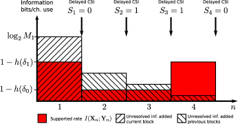
Figure 1: Variable-length transmission scheme based on delayed CSIT.

II The Block-Fading model

We consider a single-user binary channel with block-fading. The channel has two states in which it acts as binary symmetric channels (BSC) with different crossover probabilities. Transmissions to the receiver are done in blocks, each consisting of $T$ channel uses, where $T$ models the coherence time of the block-fading channel. The blocks are enumerated $n\in\mathbb{N}$, where $\mathbb{N}$ is the set of natural numbers, and the channel input in the $n$-th block is denoted $\mathbf{X}_{n}\in\mathcal{X}=\{0,1\}^{T}$. The binary channel state in the $n$-th block, denoted by $S_{n}\in\{0,1\}$, is a random variable that is independent of any previous channel states and distributed according to $\text{Pr}\left[S_{n}=1\right]=1-\text{Pr}\left[S_{n}=0\right]=q$, $q\in[0,1]$. In state $s\in\{0,1\}$, the channel acts as a BSC with crossover probability $\delta_{s}\in[0,\frac{1}{2}]$ such that receiver obtains $\mathbf{Y}_{n}=\mathbf{X}_{n}\oplus\mathbf{Z}_{n}\in\mathcal{Y}=\{0,1\}^{T}$ where $\oplus$ denotes the XOR operation and $\mathbf{Z}_{n}\in\{0,1\}^{T}$ is a binary noise vector with iid entries distributed as $\text{Bern}(\delta_{s})$. For the remaining part of this paper, we assume, without loss of generality, that $\delta_{1}<\delta_{0}$. Note that the state with $\delta_{0}$ can also be used to model a block with intermittent interference. The receiver knows $S_{n}$ when $\mathbf{X}_{n}$ is sent, but the transmitter learns it after it is sent, at the end of the $n$-th block. Thus the channel state $S_{n}$ may be used to adapt the transmission scheme from the $(n+1)$-th block. Moreover, we consider a stop-feedback setting in which the receiver feeds back noiseless ACK/NACK to the transmitter that indicates termination. The capacity of the described channel is $C=1-qh_{b}(\delta_{1})-(1-q)h_{b}(\delta_{0})$, where $h_{b}(\cdot)$ is the binary entropy function. The capacity is approached by fixed-length codes, with blocklengths tending to infinity. As shown in Section V, binary fading markedly degrades the performance at finite blocklength.

II-A Fixed-length block codes

The achievable rates using fixed-length block codes may be approximated by (1), where the dispersion of the block-fading model described (per channel use) can be shown to be [4]

$$V =\mathbb{E}\left[\delta_{S}(1-\delta_{S})\left(\log\frac{1-\delta_{S}}{\delta_{S}}\right)^{2}\right]$$

$$\quad+Tq(1-q)(h_{b}(\delta_{0})-h_{b}(\delta_{1}))^{2},$$ (2)

with the expectation taken over the channel state $S\in\{0,1\}$.

II-B Variable-length codes

For fading channels with CSI at the receiver (CSIR) and delayed CSIT, variable-length coding can be achieved either through stop-feedback as in [2, Theorem 3] or delayed CSIT. With stop-feedback, the transmitter sends incremental redundancy until an ACK is obtained, while the receiver makes an estimate of the correct codeword in each block and if the reliability of the estimate is higher than $1-\epsilon$, the receiver feeds back an ACK that terminates the transmission. This scheme is referred to as variable-length stop-feedback (VLSF) coding. On the other hand, delayed CSIT can be used by the transmitter to estimate whether the receiver has collected enough information density and thereby terminate the transmission. This communication scheme is referred to as variable-length coding with delayed CSIT (VLD).

The achievable rates of these communication schemes can be computed using the Theorem 3 in [2] and the dependency testing bound in [1], respectively. In Fig. 1, the VLD scheme is illustrated for the block-fading model described previously. Initially, the transmitter chooses a codeword from a codebook of $M_{1}$ codewords. In each block, the receiver collects information density that resolves some uncertainty about the correct codeword. After the transmission, the transmitter obtains the CSI of the previous block, and using the dependency testing bound in [1], computes the probability of error $\hat{\epsilon}$. If $\hat{\epsilon}<\epsilon$, the transmitter terminates the transmission, while it sends additional incremental redundancy otherwise. This continues until the amount of information density allows the receiver to reliably decode the message. As shown in the specific realization in Fig. 1, variable-length coding with periodic feedback eventually leads to cases where the receiver collects a wasteful amount of information density.

III Expandable Message Space Codes

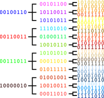
(a) Tree of codewords.

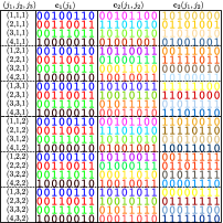
(b) List of codewords.

Figure 2: Depicts a random binary tree codebook and the corresponding list of codewords where $\mathcal{X}=\{0,1\}^{8}$ and message cardinalities $M_{1}=4$, $M_{2}=3$ and $M_{3}=2$. Note that equal blocks have the same colors.

This section describes the EMS codes and EMS stop-feedback (EMS-SF) codes. In contrast to fixed-length block codes, EMS codes allow the number of codewords in each block to expand in a tree-like fashion. Two types of codes are introduced which allow the message space to expand in each block and are analogous to fixed-length block codes and VLSF codes in [2], respectively. In the following, $M_{i}^{k}$ denotes $\prod_{n=i}^{k}M_{n}$ for $k\geq i$ and $1$ otherwise. An $((M_{1},\ldots,M_{N}),\epsilon)$ EMS code consists of

• $N$ message sets, $\mathcal{M}_{n}=\{1,\ldots,M_{n}\}$, $n\in\{1,\ldots,N\}$,

• a set of encoding functions $\mathbf{c}_{n}:\mathcal{M}_{1}\times\ldots\times\mathcal{M}_{n}\rightarrow\mathcal{X}$,

• a decoder function $\mathbf{g}:\mathcal{Y}^{N}\rightarrow\mathcal{M}_{1}\times\ldots\times\mathcal{M}_{N}\cup\{\mathrm{e}\}$ that assigns estimates $\hat{j}_{1},\ldots,\hat{j}_{N}$ or an error message $\mathrm{e}$ to each received sequence $\mathbf{y}^{N}$,

s.t. the average error probability $\text{Pr}\left[\mathbf{g}(\mathbf{Y}^{N})\not=(J_{1},\ldots,J_{N})\right]\leq\epsilon$, where $J_{1}\in\mathcal{M}_{1},\ldots,J_{N}\in\mathcal{M}_{N}$ denote the transmitted equiprobable messages.

In particularly, we denote a codeword of an EMS code as $\mathbf{c}(j_{1},\ldots,j_{N})\in\mathcal{X}^{N}$, with $(j_{1},\ldots,j_{N})\in(\mathcal{M}_{1},\ldots,\mathcal{M}_{N})$, and $\mathbf{c}_{i}^{k}(j_{1},\ldots,j_{N})\in\mathcal{X}^{k-i+1}$, $k\geq i$, denote the $i$-th to the $k$-th block of $\mathbf{c}(j_{1},\ldots,j_{N})$. As opposed to a traditional fixed-length block code with $\prod_{i=1}^{N}M_{i}$ messages, the EMS codes differ only by the definition of the encoder functions that restricts the $n$-th block to only depend on the messages $M_{1},\ldots,M_{n}$. This property implies that the codewords of an EMS code have a tree-like overlapping structure such that

$$\mathbf{c}_{1}^{n}(j_{1},\ldots,j_{n},j_{n+1},\ldots,j_{N})=\mathbf{c}_{1}^{n}(j_{1},\ldots,j_{n}),$$ (3)

for $(j_{n+1},\ldots,j_{N})\in(\mathcal{M}_{n+1},\ldots,\mathcal{M}_{N})$, and hence we can uniquely denote $\mathbf{c}_{1}^{n}(j_{1},\ldots,j_{N})$ by $\mathbf{c}(j_{1},\ldots,j_{n})$.

Next, we define an EMS code that takes advantage of stop-feedback. An $(l,(M_{1},\ldots,M_{N}),\epsilon)$ EMS-SF code consists of

• $N$ message sets $\mathcal{M}_{n}\in\{1,\ldots,M_{n}\}$, $n\in\{1,\ldots,N\}$,

• a sequence of encoders $\mathbf{c}^{SF}_{n}:\mathcal{M}_{1}\times\ldots\times\mathcal{M}_{n^{\prime}}\rightarrow\mathcal{X}$, where $n^{\prime}=\min(n,N)$,

• a sequence of decoders $\mathbf{g}^{SF}_{n}:\mathcal{Y}^{n}\rightarrow\mathcal{M}_{1}\times\ldots\times\mathcal{M}_{n^{\prime}}$, that assigns the best estimates $\hat{j}_{1},\ldots,\hat{j}_{n^{\prime}}$ at time $n$ for each possible sequence in $\mathcal{Y}^{n}$,

• a random variable $\tau^{*}\in\mathbb{N}$ satisfying $\mathbb{E}\left[\tau^{*}\right]\leq l$,

s.t. $\text{Pr}\left[\mathbf{g}^{SF}_{\tau^{*}}(Y^{\tau})\not=(J_{1},\ldots,J_{{\tau^{*}}^{\prime}})\right]\leq\epsilon$, ${\tau^{*}}^{\prime}=\min(\tau^{*},N)$, where $J_{1}\in\mathcal{M}_{1},\ldots,J_{N}\in\mathcal{M}_{N}$ denotes the equiprobable messages.

Although $N$ message sets are defined for the EMS-SF codes, the transmission may be terminated before all messages have been decoded without declaring an error. When $M_{n}=1$ for $n\geq 2$, the EMS code and EMS-SF are identical to traditional a fixed-length block code and a VLSF code with $M_{1}$ messages, respectively. The overlapping property allows EMS and EMS-SF codes to be built online, based on common randomness, according to feedback or CSI after each block. A practical EMS example are the rate-compatible convolutional codes in which new source bits only affect the future states.

To illustrate how EMS codes can be used in variable-length coding on a binary block-fading channel with $T=8$, consider the example on Fig. 2. Assume that from a codebook of $M_{1}=4$ codewords, the transmitter initially transmits a codeword with index $j_{1}\in\{1,2,3,4\}$. After the transmission, the transmitter obtains delayed CSIT and finds that the codeword can not be decoded reliably at the receiver. Instead of sending incremental redundancy, the transmitter chooses to expand the message space by a factor of $M_{2}=3$ and injects a new message $j_{2}\in\{1,2,3\}$. Fig. 2(a) depicts how the codebook expands. To send the second block, the encoder $\mathbf{c}_{2}(j_{1},j_{2})$ is used, and hence the second transmitted block depends on both $j_{1}$ and $j_{2}$. The dependency on $j_{1}$ essentially combines the injected message $j_{2}$ and the incremental redundancy for the first message $j_{1}$. Note that if $M_{2}$ had been $1$, purely incremental redundancy would have been send. Upon obtaining the CSI of the second block, the transmitter injects another message $j_{3}\in\{1,2\}$ using the encoder $\mathbf{c}_{3}(j_{1},j_{2},j_{3})$, and finally the CSI allows reliable decoding. The codebook of $M_{1}M_{2}M_{3}=24$ codewords generated through this process is shown in Fig 2(b).

For the remaining results, we use random codebooks with iid entries drawn from a $\text{Bern}(\frac{1}{2})$ distribution.

In order to provide a non-asymptotic characterization of the achievable rates of the EMS codes, we state the following bound, analogous to the dependency testing bound in [1].

Theorem 1.

The error probability for $((M_{1},\ldots,M_{N}),\epsilon)$ EMS code is bounded as

$$\epsilon \leq\text{Pr}\left[i(\mathbf{X}_{1}^{N};\mathbf{Y}_{1}^{N})\leq\log\frac{M_{1}^{N}-1}{2}\right]$$

$$\quad+\sum_{n=1}^{N}\frac{M_{n+1}^{N}(M_{n}-1)}{2}$$

$$\qquad\qquad\text{Pr}\left[i(\mathbf{X}_{1}^{N};\mathbf{Y}_{1}^{n-1},\overline{\mathbf{Y}}_{n}^{N})>\log\frac{M_{1}^{N}-1}{2}\right],$$ (4)

where $\mathbf{X}_{i}$ is distributed according to the channel input distribution and $\mathbf{Y}_{i}$ and $\overline{\mathbf{Y}}_{i}$ are distributed according to the output distribution, conditioned and unconditioned on the channel input, respectively.

Proof.

See Appendix A. ∎

The result in Theorem 1 can be equivalently stated as

Proposition 1.

The error probability for $((M_{1},\ldots,M_{N}),\epsilon)$-code EMS code is

$$\epsilon \leq\sum_{n=1}^{N}\frac{M_{n+1}^{N}(M_{n}-1)}{M_{1}^{N}-1}$$

$$\qquad\mathbb{E}\left[\exp{\left\{i(\mathbf{X}_{1}^{n-1};\mathbf{Y}_{1}^{n-1})-\left|i(\mathbf{X}_{1}^{N};\mathbf{Y}_{1}^{N})-\log\frac{M_{1}^{N}-1}{2}\right|^{+}\right\}}\right].$$ (5)

Proof.

See Appendix B. ∎

Next, we consider a non-asymptotic bound for EMS-SF codes. This generalizes the VLSF code from [1].

Theorem 2.

Fix $\gamma_{n}$ for $n\in\{1,\ldots,N\}$ and set $\gamma_{n}=0$ for $n>N$. Let $\mathbf{X}_{i}$ and $\overline{\mathbf{X}}_{i}$ be independent copies of the same process and $\mathbf{Y}_{i}$ be the output of the channel when $\mathbf{X}_{i}$ is its input. Define the hitting times

$$\tau =\inf\left\{k\geq 1:i(\mathbf{X}_{1}^{k};\mathbf{Y}_{1}^{k})\geq\sum_{i=1}^{k}\gamma_{i}\right\}$$ (6)

$$\overline{\tau}_{n} =\inf\left\{k\geq n:i(\mathbf{X}_{1}^{n-1};\mathbf{Y}_{1}^{n-1})+i(\mathbf{\overline{X}}_{n}^{N};\mathbf{Y}_{n}^{N})\geq\sum_{i=1}^{k}\gamma_{i}\right\},$$ (7)

Then for any tuple $(M_{1},\ldots,M_{N})$ there exists an $(l,(M_{1},\ldots,M_{N}),\epsilon)$ EMS-SF code such that

$$l\leq\mathbb{E}\left[\tau\right]\quad\text{and}\quad\epsilon\leq\mathbb{E}\left[\sum_{n=1}^{\min(\tau,N)}\tilde{M}^{\tau}_{n}\text{Pr}\left[\overline{\tau}_{n}\leq\tau\right]\right].$$ (8)

where $\tilde{M}_{k}^{n}=(M_{k}-1)M_{k+1}^{\min(N,n))}$.

Proof.

See Appendix C. ∎

The achievable rate is then computed as $R^{*}(\epsilon)=\frac{\mathbb{E}\left[\sum_{n=1}^{\min(\tau,N)}\log M_{n}\right]}{\mathbb{E}\left[\tau\right]}$. To enable efficient computation of the bound in Theorem 2, we loosen the bound on the error probability (8) as follows

$$\epsilon \leq\mathbb{E}\left[\sum_{l=1}^{\tau}\tilde{M}^{\tau}_{l}\text{Pr}\left[\overline{\tau}_{l}\leq\tau\right]\right]$$ (9)

$$=\sum_{n=1}^{\infty}\text{Pr}\left[\tau=n\right]\sum_{l=1}^{n}\tilde{M}_{l}^{n}\mathbb{E}\left[\mathbbm{1}\left\{\tau\leq n\right\}\exp\{-i(X_{l}^{n};Y_{l}^{n})\}\right]$$ (10)

$$\leq\sum_{n=1}^{\infty}\text{Pr}\left[\tau=n\right]\sum_{l=1}^{n}\tilde{M}_{l}^{n}\exp\left\{-\sum_{i=l}^{n}\gamma_{i}\right\}$$ (11)

IV Backtrack retransmission

Algorithm 1 BRQ with delayed CSIT at the transmitter.

1:  input: $M_{1}$ and target probability of error $\epsilon$.

2:  initialize: Generate random binary codebook with $M_{1}$ codewords $\{\mathbf{c}(j_{1})\}$. Fetch $\log M_{1}$ nats, corresponding to the message $j_{1}\in\mathcal{M}_{1}$, and transmit $\mathbf{x}=\mathbf{c}(j_{1})\in\{0,1\}^{T}$.

3:  Receive the channel state $S_{1}$. Terminate if $\epsilon_{S_{1}}(\{M_{1}\})<\epsilon$.

4:  $k\leftarrow 1$

5:  repeat

6:     $k\leftarrow k+1$

7:     Compute $\tilde{\epsilon}_{k}=\epsilon_{S_{1},\ldots,S_{k-1},1}(\{M_{1},\ldots,M_{k-1},1\})$.

8:     if $\tilde{\epsilon}_{k}\leq\epsilon$ then {Expand message space}

9:        Find $M_{k}$ such that $\epsilon_{S_{1},\ldots,S_{k-1},1}(\{M_{1},\ldots,M_{k}\})=\epsilon$.

10:     else {Pure incremental redundancy}

11:        $M_{k}\leftarrow 1$

12:     end if

13:     Expand codebook by a factor of $M_{k}$ by generating $M_{k}$ codewords $\{\mathbf{c}_{k}(j_{1},\ldots,j_{k})\}_{j_{k}\in\mathcal{M}_{k}}$ for each $j_{1}\in\mathcal{M}_{1},\ldots,j_{k-1}\in\mathcal{M}_{k-1}$.

14:     Fetch $\log M_{k}$ nats and set the message $j_{k}$ accordingly. Transmit $\mathbf{x}_{k}=\mathbf{c}_{k}(j_{1},\ldots,j_{k})$.

15:     Receive the channel state $S_{k}$.

16:  until $S_{k}=1$ and $\tilde{\epsilon}_{k}\leq\epsilon$

The key idea of BRQ is to reduce the collected amount of wasteful information density by increasing the number of codewords in the codebook during transmission. At short blocklengths, this can efficiently be achieved using EMS codes. As for VLSF and VLD, we propose two different communication schemes which are based on delayed CSIT alone and a combination of delayed CSIT and stop-feedback.

IV-A BRQ with Delayed CSIT

The operation of BRQ is illustrated in Fig. 3 and the protocol at the transmitter is summarized in Algorithm 1. We assume that the transmitter and receiver have exchanged a seed to generate common randomness (for codebooks), and $\epsilon_{s_{1},\ldots,s_{k}}(\{M_{1},\ldots,M_{k}\})$ denotes the achievable error probability, computed by Theorem 1, of an EMS code with messages $M_{1},\ldots,M_{k}$ and the state sequence $s_{1},\ldots,s_{k}$ on the block-fading channel. The transmitter initiates the transmission in block $k=1$ by choosing a codeword from a random codebook of $M_{1}$ codewords. By the end of the $k$-th block, the CSI $s_{k}$ is obtained at the transmitter. Based on the CSI $s_{1},\ldots,s_{k}$, the objective of the transmitter is to ensure that the decoder will not collect wasteful information density in block $k+1$. Therefore the transmitter computes the probability of error if the receiver were to decode by the end of block $k+1$ and the CSI turns out to be $S_{k+1}=1$. This probability of error is given by $\tilde{\epsilon}_{k+1}=\epsilon_{s_{1},\ldots,s_{k},1}(M_{1},\ldots,M_{k},1)$. If $\tilde{\epsilon}_{k+1}<\epsilon$, higher reliability than necessary is achieved if $S_{k+1}=1$, and the message space is thus expanded by a factor of $M_{k+1}$. $M_{k+1}$ is computed such that, if $S_{k+1}=1$, then the messages $M_{1},\ldots,M_{k+1}$ can be jointly decoded with a probability of error $\epsilon$, i.e. $\epsilon_{S_{1},\ldots,S_{k},1}(M_{1},\ldots,M_{k},M_{k+1})=\epsilon$. Otherwise, $M_{k+1}$ is set to $1$, and purely incremental redundancy is send. Termination occurs when $\epsilon_{s_{1},\ldots,s_{k}}(M_{1},\ldots,M_{k})\leq\epsilon$. Since the transmitter only uses delayed CSIT, the transmitter and receiver may generate the same codebooks using common randomness.

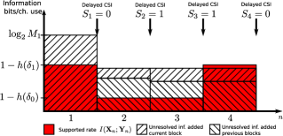
Figure 3: Operation of BRQ.

IV-B BRQ with Delayed CSIT and Stop-Feedback

When both stop-feedback and delayed CSIT is available at the transmitter, the proposed BRQ scheme is similar to Algorithm 1 but uses an EMS-SF code. However, for stop-feedback codes, the receiver decides whether to decode based on its received signal $\mathbf{Y}^{n}$ or, for the codes constructed in Theorem 2, when the information density surpasses a threshold. Wasteful information density is thereby reflected by an overwhelming probability of decoding in a specific block. With $\tau^{\{M_{1},\ldots,M_{k}\}}$ being the random stopping time of an $((M_{1},\ldots,M_{k}),\epsilon)$ EMS-SF code, the probability of decoding at the end of block $k$, given NACKs were received in the first $k-1$ blocks, is denoted by

$$p^{\{M_{1},\ldots,M_{k}\}}_{s_{1},\ldots,s_{k}}=\text{Pr}\left[\tau^{\{M_{1},\ldots,M_{k}\}}=k\big{|}\tau^{\{M_{1},\ldots,M_{k}\}}\geq k\right.$$

$$\qquad\qquad\qquad\qquad\qquad\left.,(S_{1},\ldots,S_{k})=(s_{1},\ldots,s_{k})\right]$$ (12)

where $s_{1},\ldots,s_{k}$ denotes the state sequence of the block-fading channel. We introduce an additional parameter $\beta$ which serves as a threshold for when to expand the message space.

Therefore, the transmitter uses the following algorithm; in slot $k$, if $p^{\{M_{1},\ldots,M_{k-1},1\}}_{s_{1},\ldots,s_{k-1},1}>\beta$, the message space is expanded by a factor of $M_{k}$ s.t. $p^{\{M_{1},\ldots,M_{k}\}}_{s_{1},\ldots,s_{k-1},1}=\beta$. Otherwise, $M_{k}$ is set to $1$. After computation of $M_{k}$, the threshold value $\gamma_{k}$ in Theorem 2 may be computed using (11) such that the receiver chooses to decode when the probability of error is less than $\epsilon$. Using this transmission protocol, the probability of error never exceeds $\epsilon$ and the probability of decoding in a specific slot does not exceed $\beta$.

V Numerical Results

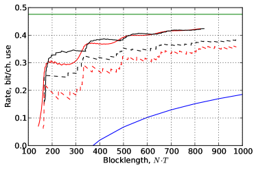
(a) $T=100$

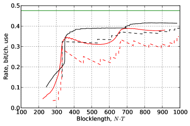
(b) $T=200$

Figure 4: Achievable rates for the block-fading model with the parameters $\delta_{1}=0.05,\delta_{0}=0.30,q=0.6$ and $\beta=0.9$. Green: capacity, black (solid): BRQ with delayed CSIT and stop-feedback, black (dashed): BRQ with delayed CSIT, red (solid): VLSF scheme, red (dashed): VLD scheme, blue: finite-length block codes (not in plot for $T=200$).

To assess the performance of the proposed communication schemes, the achievable rates of fixed-length block codes, the VLSF scheme, the BRQ schemes are computed.

The achievable rates of fixed-length block codes are computed using the normal approximation in (1). For the remaining schemes, the achievable rates are computed using Theorem 1 and Theorem 2 and by averaging over all fading realizations for a range of $M_{1}$ values. To reduce the computational complexity of averaging, we restrict the number of message space expansions to $5$. The achievable rates are computed using the parameters $\delta_{1}=0.05$, $\delta_{0}=0.3$, $q=0.6$ and $\beta=0.9$. Computed achievable rates are shown in Fig. 4.

Observe that schemes based on variable-length coding in general outperforms the fixed-length block codes. Moreover, for the VLSF and VLD schemes, we see that periodic decoding implies that the achievable rates have decreases in some ranges of blocklengths which becomes more pronounced with higher coherence time $T$. In these ranges of blocklengths, the BRQ schemes achieve higher rates. Note that optimization over $\beta$ may yield better rates for BRQ with delayed CSIT and stop-feedback.

VI Discussion and Conclusions

In this paper, we considered binary block-fading fading channel with two states. A family of codes, EMS codes, that allows the message space to expand during transmission was introduced and we provided bounds on the probability of error. Using these codes, we proposed two transmission schemes based the backtrack retransmission scheme. Numerical results showed that the proposed communication schemes achieve better rates, for the specific parameters, than communication schemes that do not benefit from delayed CSIT.

Appendix A Proof of Theorem 1

Proof.

The proof is based on the proof of the DT-bound in [1].

Codebook generation: Generate the random codebook according to the following algorithm:

1. Let $n=1$. Generate $M_{1}$ codewords $\mathbf{c}(j_{1})\in\mathcal{X}$ for $j_{1}\in\mathcal{M}_{1}$ according to the distribution $P_{\mathbf{X}_{1}}$.

2. For each tuple $(j_{1},\ldots,j_{n})\in(\mathcal{M}_{1},\ldots,\mathcal{M}_{n})$, generate $M_{n+1}$ codewords $\mathbf{c}_{n+1}(j_{1},\ldots,j_{n+1})\in\mathcal{X}$ according to the distribution $P_{\mathbf{X}_{n+1}}$.

3. Let $n=n+1$. If $n<N$, goto step 2, otherwise stop.

Encoder: The transmitter maps the message $(j_{1},\ldots,j_{N})\in(\mathcal{M}_{1},\ldots,\mathcal{M}_{L})$ to the codeword $\mathbf{c}(j_{1},\ldots,j_{N})$ which is transmitted.

Decoder: The decoder uses the Feinstein suboptimal decoder [1]. Let $\{Z_{\mathbf{x}^{N}}\}$, $\mathbf{x}^{N}\in\mathcal{X}^{N}$, be a collection of functions defined as

$$Z_{\mathbf{x}^{N}}(\mathbf{y}^{N})=\mathbbm{1}\left\{i(\mathbf{x}^{N};\mathbf{y}^{N})>\log\frac{M_{1}^{N}-1}{2}\right\}.$$ (13)

These functions are likelihood ratio hypothesis tests. The decoder runs through all $\prod_{n=1}^{N}M_{n}$ codewords and performs likelihood ratio hypothesis tests, and the codeword corresponding to the lowest index such that $Z_{\mathbf{x}^{N}}(\mathbf{y}^{N})=1$ is output.

An ordering of the codewords $\{\mathbf{c}(j_{1},\ldots,j_{N})\}$ is defined such that $\mathbf{c}_{j}=\mathbf{c}(j_{1},\ldots,j_{N})$ if and only if

$$j_{1}+\sum_{n=2}^{N}M_{1}^{n-1}(j_{n}-1)=j,$$ (14)

for $j\in\{1,\ldots,M_{1}^{N}\}$. This ordering corresponds to the codebook shown in Fig. 2(b). The conditional probability of error given that the $j$-th codeword was sent is

$$\text{Pr}\left[\{Z_{\mathbf{c}_{j}}(\mathbf{Y}^{N})=0\}\cup\bigcup_{i<j}\{Z_{\mathbf{c}_{i}}(\mathbf{Y}^{N})=1\}\big{|}\mathbf{X}^{N}=\mathbf{c}_{j}\right]$$ (15)

$$\quad=\text{Pr}\left[i(\mathbf{c}_{j};\mathbf{Y}^{N})\leq\log\frac{M_{1}^{N}-1}{2}\big{|}\mathbf{X}^{N}=\mathbf{c}_{j}\right]$$

$$\qquad+\sum_{i<j}\text{Pr}\left[i(\mathbf{c}_{i};\mathbf{Y}^{N})>\log\frac{M_{1}^{N}-1}{2}\big{|}\mathbf{X}^{N}=\mathbf{c}_{j}\right].$$ (16)

By symmetry in the codebook, (16) can be written as

$$\leq\text{Pr}\left[i(\mathbf{X}^{N};\mathbf{Y}^{N})\leq\log\frac{M_{1}^{N}-1}{2}\right]$$

$$\quad+\sum_{n=0}^{N-1}j^{\prime}_{n}\text{Pr}\left[i(\mathbf{X}^{N};\mathbf{Y}_{1}^{n},\overline{\mathbf{Y}}_{n+1}^{N})>\log\frac{M_{1}^{N}-1}{2}\right]$$ (17)

where

$$j^{\prime}_{N-1} =\left\lfloor\frac{j-1}{M_{1}^{N-1}}\right\rfloor$$ (18)

$$j^{\prime}_{n} =\left\lfloor\frac{j-1}{M_{1}^{n}}\right\rfloor-\left\lfloor\frac{j-1}{M_{1}^{n+1}}\right\rfloor\text{ for }n\in\{1,\ldots,N-2\}$$ (19)

$$j^{\prime}_{0} =j-1-\left\lfloor\frac{j-1}{M_{1}}\right\rfloor$$ (20)

Intuitively, $j^{\prime}_{l}$ describes the number of codewords among the indices $\{1,\ldots,j-1\}$ that shares the first $n$ blocks with the transmitted codeword $\mathbf{c}_{j}$.

Note that we have

$$\frac{1}{M_{1}^{N}}\sum_{j=1}^{M_{1}^{N}}\left\lfloor\frac{j-1}{M_{1}^{n}}\right\rfloor =\frac{1}{M_{n+1}^{N}}\sum_{k=1}^{M_{n+1}^{N}}(k-1)$$ (21)

$$=\frac{M_{n+1}^{N}-1}{2}$$ (22)

and

$$\frac{M_{n+1}-1}{2}-\frac{M_{n+2}^{N}-1}{2} =\frac{M_{n+2}^{N}\left(M_{n+1}-1\right)}{2}.$$ (23)

Thus by averaging over (17) with respect to $j$ and by using (22) and (23), we obtain the upper bound in (4) on the probability of error. ∎

Appendix B Proof of Proposition 1

Proof.

Note that we can write (4) as

$$\epsilon\leq\sum_{n=1}^{N}\frac{M_{n+1}^{N}(M_{n}-1)}{M_{1}^{N}-1}$$

$$\qquad\mathbb{E}\left[\left(\text{Pr}\left[i(\mathbf{X}_{1}^{N};\mathbf{Y}_{1}^{N})<\log\frac{M_{1}^{N}-1}{2}\right]\right.\right.$$

$$\qquad\quad\left.\left.+\frac{M_{1}^{N}-1}{2}\text{Pr}\left[i(\mathbf{X}_{1}^{n-1};\mathbf{Y}_{1}^{n-1})+i(\mathbf{X}_{n}^{N};\overline{\mathbf{Y}}_{n}^{N})\right.\right.\right.$$

$$\qquad\qquad\qquad\qquad\qquad\qquad\left.\left.\left.\geq\log\frac{M_{1}^{N}-1}{2}\right]\right)\right].$$ (24)

Using the identity

$$e^{\rho}\exp\left\{-\left|\log\frac{ze^{\rho}}{\gamma}\right|^{+}\right\}=\mathbbm{1}\left(z\leq\frac{\gamma}{e^{\rho}}\right)+\frac{\gamma}{z}\mathbbm{1}\left(z>\frac{\gamma}{e^{\rho}}\right),$$ (25)

by setting $z=\frac{dP_{\mathbf{X}_{n}\ldots,\mathbf{X}_{N},\mathbf{Y}_{n},\ldots,\mathbf{Y}_{N}}}{d(P_{\mathbf{X}_{n}\ldots,\mathbf{X}_{N}}\times P_{\mathbf{Y}_{n},\ldots,\mathbf{Y}_{N}})}$ and by averaging both sides of (25) with respect to the joint pmf $P_{\mathbf{X}_{n}\ldots,\mathbf{X}_{N},\mathbf{Y}_{n},\ldots,\mathbf{Y}_{N}}$, we obtain

$$\mathbb{E}\left[\exp\left\{\rho-\left|i(\mathbf{X}_{n}^{N};\mathbf{Y}_{n}^{N})+\rho-\log\gamma\right|^{+}\right\}\right]$$

$$\qquad=\text{Pr}\left[i(\mathbf{X}_{n}^{N};\mathbf{Y}_{n}^{N})+\rho\leq\log\gamma\right]$$

$$\qquad\quad+\gamma\text{Pr}\left[i(\mathbf{X}_{n}^{N};\overline{\mathbf{Y}}^{N}_{n})+\rho>\log\gamma\right].$$ (26)

Substituting (26) into (24) yields the bound in (5). ∎

Appendix C Proof of Theorem 2

Proof.

The proof is similar to the proof of Theorem 3 in [2].

A codebook, shared by the transmitter and receiver, with $M_{1}^{N}$ infinite dimensional codewords drawn from the distribution $P_{\mathbf{X}_{n}}$ such that

$$\mathbf{c}_{n}(j_{1},\ldots,j_{N}) \in\mathcal{X}$$ (27)

for $(j_{1},\ldots,j_{N})\in(\mathcal{M}_{1},\ldots,\mathcal{M}_{N})$ and $n\in\mathbb{N}$. Additionally, the codebook has the following property

$$\mathbf{c}_{n}(j_{1},\ldots,j_{n}) =\mathbf{c}_{n}(j_{1},\ldots,j_{N})\in\mathcal{X}$$ (28)

and $n\in\{1,\ldots,N\}$. As for the EMS codes, this property implies that

$$\mathbf{c}_{n}(j_{1},\ldots,j_{k},j_{k+1},\ldots,j_{N})=\mathbf{c}_{n}(j_{1},\ldots,j_{k},j^{\prime}_{k+1},\ldots,j^{\prime}_{N})$$ (29)

for $k\in\{1,\ldots,N-1\}$, $(j_{k+1}^{\prime},\ldots,j_{N}^{\prime})\in(\mathcal{M}_{k+1},\ldots,\mathcal{M}_{N})$ and $n\in\{1,\ldots,k\}$.

The $(l,(M_{1},\ldots,M_{N}),\epsilon)$ EMS-SF code is defined by a sequence of encoders $\mathbf{c}^{SF}_{n}:\mathcal{M}_{1}\times\ldots,\mathcal{M}_{n^{\prime}}\rightarrow\mathcal{X}$ that maps the messages $j_{1},\ldots,j_{n^{\prime}}$ to the channel input $\mathbf{c}_{n}(j_{1},\ldots,j_{n^{\prime}})$, where $n^{\prime}=\min(n,N)$. By the end of the $n$-th block, the decoder computes the $M_{1}^{n^{\prime}}$ information densities

$$S_{n}(j_{1},\ldots,j_{n^{\prime}}) =\sum_{k=1}^{n}i(\mathbf{c}^{SF}_{k}(j_{1},\ldots,j_{n^{\prime}});\mathbf{Y}_{k})$$ (30)

for $(j_{1},\ldots,j_{n^{\prime}})\in(\mathcal{M}_{1},\ldots,\mathcal{M}_{n^{\prime}})$.

Define the events $E_{n}(j_{1},\ldots,j_{n^{\prime}})=\left\{S_{n}(j_{1},\ldots,j_{n^{\prime}})\geq\sum_{i=1}^{n^{\prime}}\gamma_{i}\right\}$ and the stopping times

$$\tau_{j_{1},\ldots,j_{n}} =\inf\left\{k\geq 1,\exists(j_{n+1},\ldots,j_{N})\in(\mathcal{M}_{n+1},\ldots,\mathcal{M}_{N})\right.$$

$$\qquad\qquad\qquad\left.:E_{k}(j_{1},\ldots,j_{n})\right\}$$ (31)

for $n<N$ and otherwise

$$\tau_{j_{1},\ldots,j_{N}}=\inf\left\{k\geq 1:E_{k}(j_{1},\ldots,j_{N})\right\}.$$ (32)

We define the moment of the first upcrossing as

$$\tau^{*}=\min\{n\geq 1:\exists j_{1},\ldots,j_{n^{\prime}},E_{n}(j_{1},\ldots,j_{n^{\prime}})\},$$ (33)

and the decoder is given by

$$\mathbf{g}^{SF}_{\tau^{*}}(\mathbf{Y}^{\tau^{*}})$$

$$=\max\{(j_{1},\ldots,j_{{\tau^{*}}^{\prime}})\in(\mathcal{M}_{1},\ldots,\mathcal{M}_{{\tau^{*}}^{\prime}})$$

$$\qquad\qquad:\tau_{j_{1},\ldots,j_{{\tau^{*}}^{\prime}}}=\tau^{*})\},$$ (34)

where ${\tau^{*}}^{\prime}=\min(\tau^{*},N)$ and $\max(\cdot)$ returns the tuple attaining the maximum in lexicographical order. The average transmission length is bounded as

$$\mathbb{E}\left[\tau^{*}\right] \leq\sum_{n=1}^{\infty}\frac{1}{M_{1}^{n^{\prime}}}\sum_{\stackrel{{\scriptstyle(j_{1},\ldots,j_{n^{\prime}})\in}}{{(\mathcal{M}_{1},\ldots,\mathcal{M}_{n^{\prime}})}}}\text{Pr}\left[\tau_{j_{1},\ldots,j_{n^{\prime}}}=n|J_{1}=j_{1},\ldots,J_{n^{\prime}}=j_{n^{\prime}}\right]$$ (35)

$$=\sum_{n=1}^{\infty}\text{Pr}\left[\tau_{1,\ldots,1}=n|J_{1}=1,\ldots,J_{n^{\prime}}=1\right]$$ (36)

$$=\mathbb{E}\left[\tau\right].$$ (37)

where (37) follows from the definition of $\tau$ in (6). Finally, the probability of error is bounded as following

$$\text{Pr}\left[\mathbf{g}^{SF}_{\tau^{*}}(\mathbf{Y}^{\tau^{*}})\not=(J_{1},\ldots,J_{{\tau^{*}}^{\prime}})\right]$$ (38)

$$\quad=\mathbb{E}_{\tau^{*}}\left[\text{Pr}\left[\mathbf{g}^{SF}_{\tau^{*}}(\mathbf{Y}^{\tau^{*}})\not=(J_{1},\ldots,J_{{\tau^{*}}^{\prime}})|\tau^{*}\right]\right]$$ (39)

$$\quad\leq\mathbb{E}_{\tau^{*}}\left[\text{Pr}\left[\mathbf{g}^{SF}_{\tau^{*}}(\mathbf{Y}^{\tau^{*}})\not=(\underbrace{1,\ldots,1}_{{\tau^{*}}^{\prime}\text{ times}})|J_{1}=1,\ldots,J_{{\tau^{*}}^{\prime}}=1,\tau^{*}\right]\right]$$ (40)

$$\quad\leq\mathbb{E}_{\tau^{*}}\left[\text{Pr}\left[\tau_{\underbrace{1,\ldots,1}_{{\tau^{*}}^{\prime}\text{ times}}}\geq\tau^{*}|J_{1}=1,\ldots,J_{{\tau^{*}}^{\prime}}=1,\tau^{*}\right]\right]$$ (41)

$$\quad\leq\mathbb{E}\left[\sum_{\stackrel{{\scriptstyle j_{1}\in\mathcal{M}_{1},\ldots,j_{{\tau^{*}}^{\prime}}\in\mathcal{M}_{{\tau^{*}}^{\prime}}}}{{(j_{1},\ldots,j_{{\tau^{*}}^{\prime}})\not=(1,\ldots,1)}}}\mathbbm{1}\{\tau_{j_{1},\ldots,j_{{\tau^{*}}^{\prime}}}\leq\tau_{1,\ldots,1}\}\right.$$

$$\qquad\qquad\qquad\qquad\qquad\qquad\left.|J_{1}=1,\ldots,J_{{\tau^{*}}^{\prime}}=1\right]$$ (42)

$$\quad=\mathbb{E}\left[\sum_{n=1}^{{\tau^{*}}^{\prime}}\sum_{\stackrel{{\scriptstyle\stackrel{{\scriptstyle(j_{1},\ldots,j_{n-1})=(1,\ldots,1),}}{{j_{n}\in\mathcal{M}_{n},\ldots,j_{{\tau^{*}}^{\prime}}\in\mathcal{M}_{{\tau^{*}}^{\prime}}}},}}{{j_{n}\not=1}}}\mathbbm{1}\{\overline{\tau}_{n}\leq\tau\}\right]$$ (43)

$$\quad=\mathbb{E}\left[\sum_{n=1}^{{\tau^{*}}^{\prime}}(M_{n}-1)M_{n+1}^{{\tau^{*}}^{\prime}}\mathbbm{1}\{\overline{\tau}_{n}\leq\tau\}\right],$$ (44)

where (40) follows from (34), (42) from the union bound and (43) from the definition of $\overline{\tau}_{n}$ in (7). Lastly, (8) follows from the fact that ${\tau^{*}}^{\prime}\leq\min(\tau,N)$, which completes the proof. ∎

References

- [1] Y. Polyanskiy, H. V. Poor, and S. Verdu, “Channel coding rate in the finite blocklength regime,” IEEE Trans. Inform. Theory, vol. 56, no. 5, pp. 2307–2359, 2010.
- [2] ——, “Feedback in the non-asymptotic regime,” IEEE Trans. Inform. Theory, vol. 57, no. 8, pp. 4903–4925, 2011.
- [3] W. Yang, G. Durisi, T. Koch, and Y. Polyanskiy, “Quasi-static simo fading channels at finite blocklength,” in IEEE International Symposium on Information Theory Proceedings, 2013, pp. 1531–1535.
- [4] Y. Polyanskiy and S. Verdu, “Scalar coherent fading channel: Dispersion analysis,” in IEEE International Symposium on Information Theory Proceedings, 2011, pp. 2959–2963.
- [5] W. Yang, G. Durisi, T. Koch, and Y. Polyanskiy, “Block-fading channels at finite blocklength,” in Proceedings of the Tenth International Symposium on Wireless Communication Systems, 2013, pp. 1–4.
- [6] P. Popovski, “Delayed channel state information: Incremental redundancy with backtrack retransmission,” in IEEE International Communication Conference, Jun. 2014, accepted for publication.