Probing Quintessence Potential
with Future Cosmological Surveys

Yoshitaka Takeuchi$\,{}^{1}$, Kiyotomo Ichiki$\,{}^{2}$, Tomo Takahashi$\,{}^{3}$,
and Masahide Yamaguchi$\,{}^{4}$

¹ Department of Physics and Astrophysics, Nagoya University, Nagoya 464-8602, Japan
² Kobayashi-Maskawa Institute for the origin of particles and the universe, Nagoya University, Nagoya 464-8602, Japan
³ Department of Physics, Saga University, Saga 840-8502, Japan
⁴ Department of Physics, Tokyo Institute of Technology, Tokyo 152-8551, Japan

Quintessence, a scalar field model, has been proposed to account for the acceleration of the Universe at present. We discuss how accurately quintessence models are discriminated by future cosmological surveys, which include experiments of CMB, galaxy clustering, weak lensing, and the type Ia SNe surveys, by making use of the conventional parameterized dark energy models. We can see clear differences between the thawing and the freezing quintessence models at more than $1\sigma$ ($2\sigma$) confidence level as long as the present equation of state for quintessence is away from $-1$ as $w_{X}\hskip 3.00003pt\raisebox{1.72218pt}{$>$}\raisebox{-3.01385pt}{$\sim$}\hskip 1.00006pt-0.95~{}(-0.90)$. However, it is found to be difficult to probe the effective mass squared for the potential in thawing models, whose signs are different between the quadratic and the cosine-type potentials. This fact may require us to invent a new estimator to distinguish quintessence models beyond the thawing and the freezing ones.

1 Introduction

Current cosmological observations indicate that the Universe is currently in an accelerating stage, which suggests that the present Universe is dominated by an enigmatic component called dark energy. Although current cosmological observations are so precise that we can have some information on its properties such as its current energy density, the equation of state and so on, we still do not know what the dark energy is. Since the identification of dark energy is one of the most important problems in contemporary science, many researches have been performed to pursue this issue and a lot of models for dark energy have been proposed (for early works, see, e.g., [1, 2, 3, 4, 5]).

Among various dark energy models, quintessence, a scalar field model with the canonical kinetic term, may be the simplest dynamical dark energy model [1, 2, 3]. The presence of such a scalar field might be well motivated by theories of particle physics such as supergravity and/or superstring, which include scalar fields with a variety of types of the potential. However, the form of potential is strongly constrained to realize the current accelerating expansion and the proposed quintessence potentials can be roughly divided into two types [6], depending on how a quintessence field evolves: freezing (tracker) and thawing types. For the freezing (tracker) type, a quintessence field moves fast in the early Universe, then “freezes” at some later time to realize its equation of state $w_{X}$ close to $-1$. A typical example of potentials in this category is the inverse power law potential [2, 7, 8]. For such a potential, it is well known that the quintessence field exhibits a tracking behavior where it traces the equation of state of the dominant background fluid (e.g., radiation and matter). This is the reason why the freezing type is sometimes called “tracker model”. On the other hand, in the thawing model, a quintessence field almost stays somewhere on the potential in the early times, during which it behaves like a cosmological constant. At later times, the quintessence field starts to “thaw” or move, that is, starts to roll down the potential [6]. The situation is quite similar to that of the inflationary dynamics. As in the case of inflation, typical potentials of this type are (positive) power law and hilltop type [9] potentials as in chaotic and new inflation models, respectively. The difference of these potentials is characterized by the sign of the effective mass squared.

In light of this consideration, if we limit ourselves to a quintessence model as dark energy, the first thing we have to do is to differentiate these two types, i.e., freezing or thawing, by using cosmological observations. Unfortunately, current observational constraints are not precise enough to discriminate these types. However, future experiments may well probe the differences and distinguish these models, which is one of the issues that we are going to address in this paper. For this purpose, we investigate constraints expected from future surveys of cosmic microwave background (CMB), galaxy clustering and galaxy lensing shear by using their auto- and cross-correlations. We also make use of future observations of type Ia supernovae (SNeIa).

In this paper we adopt typical potentials as the fiducial models of the two types of quintessence. Specifically, we consider a power-law potential for the freezing type while the quadratic and the cosine-type potentials for the thawing type models to generate mock data for future surveys. Then, the generated mock data are fitted to some phenomenological dark energy models with its equation of state $w_{X}$ being parameterized in a simple form, which have been adopted in many works. Our primary goal is, therefore, to investigate how the confidence regions look like on the plane of dark energy parameters, and to clarify whether one can differentiate the two types from future cosmological surveys.

If one can pin down the type of quintessence, i.e., freezing or thawing type, the next task is to extract the information of the potential in more detail. In particular, for the thawing type, we have two different, but representative examples of the potential such as quadratic and cosine-type potentials. One of the differences between the two is characterized by the sign of the effective mass squared. This difference is important from both theoretical and observational reasons. From the model building point of view, it is challenging to construct a quadratic potential because it must be flat beyond the Planck scale in order to dominate the energy density at late times. However, once such a potential is realized, the field can easily take a suitable value during inflation [10]. On the other hand, the hilltop (cosine) type potential [9] naturally appears as an axion potential from particle physics models. For this type of potential, the field value is not necessarily required to exceed the Planck scale thanks to the offset of the potential, although it suffers from a severe initial value problem because there is no natural reason to keep sitting on the top of the potential. Thus, it is quite important to distinguish the sign of the effective mass squared of the potentials from this viewpoint. In fact, the sign of the effective mass squared appears in the evolution equation of perturbations so that it may leave significant imprints on the large scale structure (LSS). Thus, we also investigate how accurately we can determine the effective mass squared of the potentials from the future observational data. For this purpose, we introduce a new parameterization for dark energy equation of state, in which the sign of the effective mass squared is incorporated as a free parameter.

The organization of this paper is as follows. We briefly summarize the quintessence potential for fiducial models adopted in our analyses in Sec. 2, and some phenomenological parameterizations for the dark energy equation of state are presented in Sec. 3. In Sec. 4, we summarize the procedure of our analyses. The results of the analyses are given in Sec. 5. The final section is devoted to the conclusion and summary of this paper.

2 Quintessence Scalar Field and its models

The equation of motion for a scalar field $\phi$ in a flat Universe is given by

$${\phi}^{\prime\prime}+2{\cal H}{\phi}^{\prime}+a^{2}V_{,\phi}(\phi)=0,$$ (1)

where primes denote the derivative with respect to the conformal time, ${\cal H}={a}^{\prime}/a$ is the conformal Hubble parameter, $V(\phi)$ is a potential of scalar field and $V_{,\phi}=dV/d\phi$. The energy density and pressure of a scalar field are given by

$$\rho_{\phi} = \frac{1}{2a^{2}}\phi^{\prime 2}+V(\phi)~{},$$ (2)

$$p_{\phi} = \frac{1}{2a^{2}}\phi^{\prime 2}-V(\phi)~{},$$ (3)

respectively. The ratio of the two, $w_{X}=p_{\phi}/\rho_{\phi}$, is an equation of state for a scalar field. Since we use cosmological data including the information of density fluctuations such as CMB, one also has to consider fluctuations in a quintessence field. Working in the synchronous gauge, the evolution equation for fluctuations of the quintessence field is given by

$${\delta\phi}^{\prime\prime}+2{\cal H}{\delta\phi}^{\prime}+\frac{k^{2}}{a^{2}}\delta\phi+\frac{1}{2}{h}^{\prime}\phi^{\prime}+a^{2}V_{,\phi\phi}\delta\phi=0~{},$$ (4)

where $h$ is metric perturbation in the synchronous gauge [11] and $V_{,\phi\phi}=\frac{d^{2}V}{d\phi^{2}}$. Fluctuations of density, pressure and velocity divergence of quintessence are, respectively, given by

$$\delta\rho_{\phi} = \frac{1}{a^{2}}\phi^{\prime}{\delta\phi}^{\prime}+V_{,\phi}\delta\phi~{},$$ (5)

$$\delta p_{\phi} = \frac{1}{a^{2}}\phi^{\prime}{\delta\phi}^{\prime}-V_{,\phi}\delta\phi~{},$$ (6)

$$\theta_{\phi} = k^{2}\frac{\delta\phi}{{\phi}^{\prime}}~{}.$$ (7)

As mentioned in the introduction, quintessence models can be divided into two types, i.e., thawing and freezing (tracker) ones. Although there are still some variations of the potential form for each type, as fiducial models in this paper, we adopt the following representative potentials discussed in the literature.

For the thawing quintessence model, only two types of potentials have been considered in most cases. One is a simple quadratic potential, whose explicit form is

$$V(\phi)=\frac{1}{2}m_{\phi}^{2}\phi^{2},$$ (8)

where $m_{\phi}$ is the mass for the quintessence. Since $\phi$ begins to roll down the potential at very late epoch to realize the accelerating expansion today, the mass is roughly of the order of the present Hubble parameter $H_{0}$. In addition, in order to dominate the energy density at late time, the field value $\phi$ needs to be close to the Planck value.

The other type is the cosine one of the form [9]:

$$V(\phi)=M^{4}\left(1-\cos(\phi/f_{\phi})\right).$$ (9)

This pseudo-Nambu-Goldstone boson type of potential can well be motivated from some particle physics models and has been discussed in many papers (see, e.g., [9]).

Concerning the freezing (tracker) type, although many forms of potential have been argued, most of them include inverse power law or exponential parts in the potential, which allow an attractor solution. Here we consider a typical inverse power law type of the form:

$$V(\phi)=\beta M_{\rm pl}^{4}\left(\frac{\phi}{M_{\rm pl}}\right)^{\alpha}.$$ (10)

As mentioned above, there have been many models (potentials) discussed so far. For other freezing (tracker) types, see e.g., [7]. In this paper, we take these potentials as the fiducial models for each type.

3 Dark energy parameterizations

Since we have not yet understood the nature of the dark energy, it is common to treat dark energy as an ideal fluid with a negative equation of state. Here we follow this procedure and investigate how dark energy parameters, in particular, its equation of state defined below are constrained from future surveys. Although various parameterizations for $w_{X}$ can be found in the literature, we assume three parameterizations as described below.

3.1 Parameterization I & II

One of the aims of this paper is to discriminate the freezing and the thawing models, whose equation of states decreases and increases with time, respectively. This feature can be captured by the following parameterization [12, 13], whose form is given by

$$w_{X}(a)=w_{0}+(1-a)w_{1}=w_{0}+\frac{z}{1+z}w_{1}\,\qquad{\rm(Parameterization~{}I)}.$$ (11)

It is expected that $w_{1}<0$ for the freezing model while $w_{1}>0$ for the thawing model. We call this parameterization “Parameterization I” in the following. With this equation of state $w_{X}$, one can write its energy density as

$$\rho_{X}(z)=\rho_{X0}(1+z)^{3(1+w_{0}+w_{1})}\exp\left(\frac{-3w_{1}z}{1+z}\right),$$ (12)

where $\rho_{X0}$ is the energy density of dark energy at present time. In the above parameterization, $w_{X}$ has a simple linear dependence on the scale factor $a$, but another parameterization of this type is also possible such as $w_{X}=w_{0}+w_{1}z$, where a linear dependence on a redshift $z$ is assumed [14, 15, 16] with a cutoff at some redshift to avoid large $w_{X}$ at earlier time. But in the following, we consider the parameterization of Eq. (11) as a representative one of this category.

The equations of states for the freezing and the thawing models are also characterized by the fact that $w_{X}$ is larger (smaller) in the past for the freezing (thawing) model. This feature can be directly probed by the following parameterization [17],

$$w_{X}(a)=w_{a}w_{b}\frac{a^{q}+a_{s}^{q}}{w_{b}a^{q}+w_{a}a_{s}^{q}}=w_{a}w_{b}\frac{1+\left(\frac{1+z}{1+z_{s}}\right)^{q}}{w_{b}+w_{a}\left(\frac{1+z}{1+z_{s}}\right)^{q}}\qquad{\rm(Parameterization~{}II)},$$ (13)

where the equation of state changes from $w_{b}$ to $w_{a}$ at the transition redshift $z_{s}$ with its width characterized by $q$. It is expected that $w_{b}>w_{a}$ for the freezing model while $w_{b}<w_{a}$ for the thawing model. We call this form of $w_{X}$ “Parameterization II” in this paper. The energy density of dark energy with this parameterization can be analytically given by

$$\rho_{X}(z)=\rho_{X0}(1+z)^{3(1+{w_{a}})}\left(\frac{w_{a}+w_{b}(1+z_{s})^{q}}{w_{a}(1+z)^{q}+w_{b}(1+z_{s})^{q}}\right)^{\frac{3({w_{a}-w_{b}})}{q}}.$$ (14)

3.2 Perturbation evolution and Parameterization III

The above two parameterizations are suitable for discriminating the thawing and the freezing models. Once the thawing models would be favored from future observations, the next task is to differentiate two typical thawing models, in which the signs of the effective mass squared are opposite, that is, positive and negative. Such a difference in the sign of the effective mass squared is expected to affect the evolution of the perturbations. Thus, in this subsection, we discuss what kind of parameterization is suitable for probing the sign of the effective mass squared of a quintessence field through its perturbations.

For this purpose, let us first remind ourselves how fluctuations in dark energy fluid evolve with a given equation of state $w_{X}$. Working in the synchronous gauge [11], the energy density and velocity perturbation evolutions for a general fluid with its equation of state $w_{X}$ in the CDM rest frame are given by

$${\delta}^{\prime} = -(1+w_{X})\left(\theta+\frac{{h}^{\prime}}{2}\right)-9{\cal H}^{2}(1+w_{X})(c_{\rm s}^{2}-c_{\rm a}^{2})\frac{\theta}{k^{2}}-3{\cal H}(c_{\rm s}^{2}-w_{X})\delta~{},$$ (15)

$${\theta}^{\prime} = -{\cal H}(1-3c_{\rm s}^{2})\theta+\frac{c_{\rm s}^{2}}{(1+w_{X})}k^{2}\delta-k^{2}\sigma~{},$$ (16)

where $\delta$ and $\theta$ represent density and velocity perturbations, respectively, and $\sigma$ is anisotropic stress. One can consider non-vanishing $\sigma$ for a general dark energy fluid [18], but we can safely set $\sigma=0$ for a quintessence field. Furthermore, the effective sound speed $c_{s}$, which is the sound speed defined in the dark energy rest frame, is defined through [19]

$$\frac{\delta p}{\rho}=c_{s}^{2}\delta+3{\cal H}(1+w_{X})(c_{s}^{2}-c_{a}^{2})\frac{\theta}{k^{2}}~{}.$$ (17)

For a scalar field with the canonical kinetic term, the effective sound speed is $c_{s}^{2}=1$. The adiabatic speed of sound $c_{a}$ for a fluid is given by

$$c_{\rm a}^{2}\equiv\frac{{p}^{\prime}}{{\rho}^{\prime}}=w_{X}-\frac{{w_{X}}^{\prime}}{3{\cal H}(1+w_{X})}~{}.$$ (18)

By analogy with the case of inflation, let us try to parameterize the equation of state by using its potential, which is characterized by the slow-roll parameters [20, 21]. The adiabatic sound speed Eq. (18) can be written with the scalar field $\phi$ and the potential $V$ as

$$c_{\rm a}^{2}=\frac{{p}_{\phi}^{\prime}}{{\rho}_{\phi}^{\prime}}=\frac{\dot{p}_{\phi}}{\dot{\rho}_{\phi}}=\frac{\ddot{\phi}-V_{,\phi}}{\ddot{\phi}+V_{,\phi}}=-1+2\frac{\ddot{\phi}}{\ddot{\phi}+V_{,\phi}}~{},$$ (19)

where dots denote the derivative with respect to the cosmic time. We first introduce the following function [23, 24]

$$\beta=\frac{\ddot{\phi}}{3{H}\dot{\phi}}~{}.$$ (20)

Then, using Eq. (1), $\dot{\phi}$ is written in term of $\beta$ as

$$\dot{\phi}=-\frac{V_{,\phi}}{3(1+\beta){H}}~{}.$$ (21)

When $|\beta|\ll 1$, $\ddot{\phi}$ is given by differentiating the both sides in Eq. (21) with respect to the time as

$$\ddot{\phi}\simeq\frac{V_{,\phi}V_{,\phi\phi}}{9{H}^{2}}-\frac{(1+w)V_{,\phi}}{2}=\frac{\eta V_{,\phi}}{3}-\frac{(1+w)V_{,\phi}}{2}~{},$$ (22)

where we have used $\dot{H}/{{H}^{2}}\simeq-3(1+w_{X})/2$ and $\eta$ is defined as

$$\eta\equiv\frac{V_{,\phi\phi}}{3{H}^{2}}~{},$$ (23)

which reduces to the inflationary slow-roll parameter, $\eta=V_{,\phi\phi}/V$, when ${H}^{2}\simeq V/3$. Using Eqs. (23) and (22), we can rewrite Eq. (19) as,

$$c_{\rm a}^{2} \simeq -1+2\left(\frac{\eta}{3}-\frac{1+w_{X}}{2}\right)\left(1+\frac{\eta}{3}-\frac{1+w_{X}}{2}\right)^{-1},$$ (24)

$$\simeq -1+2\left(\frac{\eta}{3}-\frac{1+w_{X}}{2}\right)\left(1-\frac{\eta}{3}+\frac{1+w_{X}}{2}+\cdots\right),$$

$$\simeq -2-w_{X}+\frac{2}{3}\eta\,.$$

From Eqs. (18) and (24), we obtain the following differential equation for $w_{X}$:

$$\frac{dw_{X}}{d\ln a}=6(1+w_{X})(1+w_{X}-\frac{1}{3}\eta).$$ (25)

Assuming $\eta$ is a constant parameter and the present value of the equation of state is $w_{X}(a_{0})=w_{0}$, then we can solve Eq. (25) as

$$w_{X}(a)=-1+\frac{1}{3}\frac{(1+w_{0})\eta}{(1+w_{0})-(1+w_{0}-\frac{\eta}{3})a^{2\eta}}\hskip 14.22636pt{\rm(Parameterization~{}III)}\,.$$ (26)

We introduce this parameterization, especially, to differentiate the sign of the effective mass squared and to distinguish the two typical thawing models.

In the following analysis, we take these three parameterizations Eqs. (11), (13), and (26) for $w_{X}$ to investigate to what extent one can differentiate the potentials of quintessence.

4 Analysis

We here summarize the method of our analysis. We use angular power spectra from CMB and large scale structure, taking auto- and cross-correlations among them to utilize the information thoroughly.

4.1 Cosmological observables

4.1.1 CMB

Integrated Sachs-Wolfe effect

The presence of dark energy or the cosmological constant causes the decay of the gravitational potential, then affects the propagation of CMB photons along the line of sight. We can observe this effect as a cumulative one, hence name the (late-time) integrated Sachs-Wolfe (ISW) effect [25]. Since the cross-correlation between CMB and LSS such as galaxy clustering and week lensing field arises due to the ISW effect, the presence of non-vanishing cross-correlation between CMB and LSS on large scales can be a signature of dark energy.

CMB temperature fluctuations on large scales mainly come from the Sachs-Wolfe effect as a primary source and the ISW effect as a secondary one at late time. Thus we can schematically write the temperature fluctuation as $\Delta T_{\rm CMB}=\Delta T_{\rm SW}+\Delta T_{\rm ISW}$. The contribution from the ISW effect $\Delta T_{\rm ISW}$ is given by

$$\frac{\Delta T_{\rm ISW}(\hat{\bf n})}{T_{\rm CMB}}=\int_{0}^{\chi_{*}}d\chi\left[{\Phi}^{\prime}(\hat{\bf n},\chi(z))-{\Psi}^{\prime}(\hat{\bf n},\chi(z))\right],$$ (27)

where $T_{\rm CMB}$ is the mean temperature of CMB, $\hat{\bf n}$ is the direction along the line of sight, $\chi$ is the comoving distance and $\chi_{*}$ denotes the comoving distance to the last scattering surface. Here $\Phi$ and $\Psi$ are the curvature perturbation and the gravitational potential, respectively, which can be related as $\Phi=-\Psi$ on subhorizon scales, and a prime denotes a derivative with respect to the conformal time.

Deep in the horizon scale, the gravitational potential can be related to matter density fluctuations in Fourier space through the Poisson equation as

$$\Phi({\bm{k}},z)=-\frac{3}{2}\frac{\Omega_{\rm m,0}H_{0}^{2}}{ak^{2}}\delta({\bm{k}},z).$$ (28)

On large scales where the the fluctuations are small $\delta({\bm{k}},z)\ll 1$ and the linear theory is valid, they can be written as $\delta({\bm{k}},z)=\delta({\bm{k}},0)D(z)/D_{0}$, where $D(z)$ is the linear growth factor normalized as $D(z)\propto a(z)$ in the matter nominated era and $D_{0}$ is the value at the present time.

CMB lensing potential

The gravitational potential produced by large-scale structures deflects CMB photons on the way propagating to us, and produces other secondary effects on CMB temperature and polarization fields (see, e.g., [26]). We can understand such effect as a displacement of patches with deflection angle ${\bm{d}}(\hat{\bf n})$ on the sphere, and the relationship between the lensed temperature anisotropy $\tilde{T}(\hat{\bf n})$ and the unlensed one $T(\hat{\bf n})$ is given by $\tilde{T}(\hat{\bf n})=T(\hat{\bf n}+{\bm{d}}(\hat{\bf n}))$. The deflection angle can be written with the lensing potential $\psi$ as ${\bm{d}}(\hat{\bf n})=\nabla\psi(\hat{\bf n})$, where $\psi$ is defined as

$$\psi(\hat{\bf n})=-2\int_{0}^{\chi_{*}}d\chi\frac{\chi_{*}-\chi}{\chi_{*}\chi}\Psi(\hat{\bf n},\chi(z)).$$ (29)

Here we take $\psi(\hat{\bf n})$ to be an observable which characterizes weak lensing effects of CMB.

The lensing potential $\psi$ can be reconstructed from both observed temperature and polarization fields with a quadratic estimator and the noise of the lensing potential can be estimated as the reconstruction error (see, e.g., [27, 28, 29]). To compute the lensing potential ($\psi$), we use a publicly available Boltzmann code CAMB [30], and modify it to include a quintessence scalar field.

4.1.2 Galaxy Clustering

We observe the distribution of galaxies as the projected galaxy over-density in photometric redshift surveys. We consider a tomographic one, in which we can separate galaxies into some redshift bins. Fluctuations of the galaxy distribution in the $i$-th redshift bin are given by

$${\rm g}_{i}(\hat{\bf n})=\int_{z_{i}}^{z_{i+1}}dz\,b_{\rm g}(z)\,{\cal N}_{i}(z)\,\delta(\hat{\bf n},z),$$ (30)

where $b_{\rm g}(z)$ is the galaxy bias, ${\cal N}_{i}(z)$ is the selection function which represents the redshift distribution of sample galaxies, and the subscript $i$ denotes a redshift bin.

For the redshift distribution of sample galaxies, we adopt the analytic formula of [34], which includes the effect of photometric redshift errors as

$$p_{i}(z_{\rm ph}|z)=\frac{1}{\sqrt{2\pi}\sigma_{z}(z)}\exp\left[-\frac{\left(z-z_{\rm ph}\right)^{2}}{2\sigma_{z}^{2}(z)}\right],$$ (31)

where $\sigma_{z}(z)$ denotes a redshift scatter systematic error and is given by

$$\sigma_{z}(z)=\sigma_{z}^{(i)}(1+z),$$ (32)

with $\sigma_{z}^{(i)}=0.03$ for each redshift bin. Then, the selection function ${\cal N}_{i}(z)$ which includes the effect of photometric redshift errors is written as

$${\cal N}_{i}(z)=\int_{z_{\rm ph}^{(i)}}^{z_{\rm ph}^{(i+1)}}dz_{\rm ph}N(z)p_{i}(z_{\rm ph}|z)=\frac{1}{2}\left[{\rm erf}(x_{i+1})-{\rm erf}(x_{i})\right]N(z),$$ (33)

where $x_{i}\equiv(z_{\rm ph}^{(i)}-z)/\sqrt{2}\sigma_{z}(z)$ and the redshift distribution of galaxy samples $N(z)$ is assumed to be [35, 36]

$$N(z)\propto z^{\alpha}\exp\left[-\left(\frac{z}{z_{0}}\right)^{\beta}\right].$$ (34)

Here $N(z)$ should be normalized as $\int N(z)dz=1$ and we adopt $\alpha=2.0$, $\beta=1.5$. $z_{0}$ is determined from the relation with mean redshift $z_{\rm m}$ defined as

$$z_{\rm m}=\int zN(z)dz.$$ (35)

We adopt the mass weighted average bias given by

$$b_{\rm g}(z)=\left.\int_{M_{\rm min}}^{\infty}b_{\rm h}(M,z)\frac{dn_{\rm h}(M,z)}{dM}dM\right/\left[\int_{M_{\rm min}}^{\infty}\frac{dn_{\rm h}(M,z)}{dM}dM\right]\,,$$ (36)

where $M_{\rm min}$ is the minimum mass of the halos which host the galaxies we can observe, $b_{\rm h}(M,z)$ and $dn_{\rm h}(M,z)/dM$ denote the halo bias and the halo mass function, respectively. We utilize the models of [31] and [32] for the halo bias and the halo mass function, respectively. In the following, we treat $M_{\rm min}$ as a model parameter to determine the galaxy bias, and also derive its constraint from mock data.

4.1.3 Galaxy weak lensing

The light path from distant galaxies is deflected by foreground large-scale structures. The effects can be observed as the magnification or the distortion of images of background galaxies (see, e.g., [33]) and the effects can be evaluated from the measurements of shear of each galaxy. Here we consider a galaxy weak lensing survey with photometric redshift. The averaged galaxy weak lensing shear is given by

$$\gamma_{i}(\hat{\bf n})=\frac{3\Omega_{\rm m0}H_{0}^{2}}{2}\int_{0}^{\infty}d\chi\frac{\chi(z)}{a(z)}\left[\int_{{\rm max}(z,z_{i})}^{z_{i+1}}dz^{\prime}\,{\cal N}_{i}(z^{\prime})\frac{\chi(z^{\prime})-\chi(z)}{\chi(z^{\prime})}\right]\delta(\hat{\bf n},\chi(z))~{},$$ (37)

where we assume a tomographic survey and the subscript $i$ denotes a redshift bin.

4.2 Angular power spectra

An observable given by the projection of the line of sight along the comoving radial coordinate $\chi$ in direction $\hat{\bf n}$ is given by

$$X({\hat{\bf n}})=\int d\chi S^{X}(\hat{\bf n}\chi,\tau_{0}-\chi),$$ (38)

where $S^{X}({\bm{k}},\tau)$ represents the source term of $X$. Assuming statistical isotropy, angular correlation between two observables $X$ and $Y$ is given by angular power spectrum as

$$\langle a_{\ell m}^{X}a_{\ell^{\prime}m^{\prime}}^{Y*}\rangle=C_{\ell}^{XY}\delta_{\ell\ell^{\prime}}\delta_{mm^{\prime}},$$ (39)

where $a_{\ell m}^{X}$ are the expansion coefficients of the observables $X(\hat{\bf n})$ in spherical harmonics, $X(\hat{\bf n})\equiv\sum_{\ell m}a_{\ell m}^{X}Y_{\ell m}(\hat{\bf n})$, and given by

$$a_{\ell m}^{X}=4\pi\ (-i)^{\ell}\int\frac{d^{3}k}{(2\pi)^{3}}Y_{\ell m}^{*}(\hat{\bf k})\int d\chi S^{X}({\bm{k}},\tau_{0}-\chi)j_{\ell}(k\chi).$$ (40)

If we write the source term as $S^{X}({\bm{k}},\tau_{0}-\chi)=S^{X}(k,\tau_{0}-\chi)\tilde{\Phi}({\bm{k}})$, then the angular power spectrum is given by

$$C_{\ell}^{XY}=\frac{2}{\pi}\int d^{3}kP_{\Phi}(k)\int d\chi S^{X}(k,\tau_{0}-\chi)j_{\ell}(k\chi)\int d\chi^{\prime}S^{Y}(k,\tau_{0}-\chi^{\prime})j_{\ell}(k\chi^{\prime}),$$ (41)

where $\tilde{\Phi}({\bm{k}})$ is the Fourier transform of the primordial curvature perturbation $\Phi(\hat{\bf n})$, $P_{\Phi}(k)$ is the power spectrum of $\Phi$, and $S^{X}(k,\tau_{0}-\chi)$ is the transfer function of $X$.

In the following analysis, we take into account all auto- and cross-correlations between different observables, except for the cross-correlations of CMB $E$-mode polarization with CMB lensing, galaxy clustering and galaxy weak lensing shear. This is because CMB $E$-mode polarizations are produced at the last scattering surface or at the epoch of reionization, whose redshifts are much larger than those probed by CMB lensing, galaxy clustering and galaxy weak lensing.

4.3 Parameter estimation with angular power spectra

In order to discuss whether we can probe the differences among quintessence models, we fit the phenomenological dark energy models based on the parameterized equation of state given in Section 3, by generating mock data of angular power spectra ${\bm{C}}_{\ell,{\rm fid}}^{\rm XY}$ for the fiducial quintessence models, with $X,Y$ representing the observables discussed above. Following [37], we evaluate $\chi^{2}$ as

$$\chi^{2}=\sum_{{\rm XY},{\rm ZW}}\sum_{\ell}\left({\bm{C}}_{\ell,{\rm fid}}^{\rm XY}-{\bm{C}}_{\ell,{\rm mod}}^{\rm XY}\right)^{\rm T}({{\bf Cov}_{\ell}})_{{\rm XY},{\rm WZ}}^{-1}\left({\bm{C}}_{\ell,{\rm fid}}^{\rm WZ}-{\bm{C}}_{\ell,{\rm mod}}^{\rm WZ}\right),$$ (42)

where ${\bm{C}}_{\ell,{\rm mod}}^{\rm XY}$ is the power spectra for the phenomenological dark energy model and $({{\bf Cov}_{\ell}})$ denotes covariance matrix. Each component of the covariance matrix is given by

$${\rm Cov}_{\ell}\left[C_{\ell,{\rm fid}}^{\rm XY},\,C_{\ell,{\rm fid}}^{\rm WZ}\right]=\frac{1}{(2\ell+1)f_{\rm sky}}\left(\tilde{C}_{\ell}^{\rm XW}\tilde{C}_{\ell}^{\rm YZ}+\tilde{C}_{\ell}^{\rm XZ}\tilde{C}_{\ell}^{\rm YW}\right),$$ (43)

with

$$\tilde{C}_{\ell}^{\rm XY}\equiv C_{\ell,{\rm fid}}^{\rm XY}+N_{\ell}^{\rm XY}.$$ (44)

Here $f_{\rm sky}$ is the sky coverage, $N_{\ell}^{\rm X}$ is the noise spectrum for the auto- or cross-correlations between the observables $X$ and $Y$. For this noise spectrum, we assume that the correlations of noises between different observables are negligible; $N_{\ell}^{\rm XY}\equiv\delta_{\rm XY}N_{\ell}^{\rm X}$.

Experiment	$f_{\rm sky}$	$\nu$	$\theta_{\rm FWHM}$	$\Delta_{\nu}^{T}$	$\Delta_{\nu}^{P}$
		[GHz]	[arcmin]	[$\mu$K/pixel]	[$\mu$K/pixel]
COrE	0.65	105	10.0’	0.536	0.926
		135	7.8’	0.674	1.167
		165	6.4’	0.834	1.441
		195	5.4’	0.974	1.681
		225	4.7’	1.123	1.945
		255	4.1’	2.966	5.122
		285	3.7’	5.459	9.405
		315	3.3’	16.30	28.24
		375	2.8’	49.00	85.00
		435	2.4’	124.0	215.0

Table 1: The specification of CMB experiment. $f_{\rm sky}$ is the sky coverage, $\theta_{\rm FWHM}$ is the beam width at FWHM, $\Delta_{\nu}^{T}$ and $\Delta_{\nu}^{P}$ represent the sensitivity of each channel to the temperature and polarization, respectively. $\nu$ indicates the channel frequency of detectors. We assume the COrE-like satellite survey, and these parameters can be found in [38].

For the CMB experiment, we assume the ideal condition in which foreground removal can be done completely and noise components depend only on detector noise. If the detector noise is Gaussian white noise, the noise spectra for the temperature and the polarization fluctuations are given by

$$N_{\ell}^{T,P}=\left[\sum_{\nu}\left\{\left(\theta_{{\rm FWHM},\nu}\Delta_{\nu}^{T,P}\right)^{-2}\exp\left(-\frac{\ell(\ell+1)\theta_{{\rm FWHM},\nu}}{8\ln 2}\right)\right\}\right]^{-1},$$ (45)

where the superscripts $T$ and $P=\{E,B\}$ denote the temperature and the polarization components, respectively, $\nu$ is the frequency at each band channel, $\Delta_{\nu}^{T,P}$ is the sensitivity of detector per pixel at $\nu$ band and $\theta_{{\rm FWHM},\nu}$ represents the resolution at $\nu$ band. The values for the COrE-like satellite are given in Table 1. On the estimation of the CMB lensing potential $\psi$, we adopt the noise spectrum of the lensing potential $N_{l}^{\psi}$ following the method in [28] optimally combining the temperature and the polarization fields. Therefore, the temperature $T$ and the E-mode polarization in our analysis are unlensed components and all information on CMB lensing is included in the lensing potential $\psi$.

The specification of the LSST survey

	survey area	sample galaxies	mean redshift	maximum redshift	redshift bin
	$f_{\rm sky}$	$\bar{n}_{\rm g}$ [arcmin-2]	$z_{\rm m}$	$z_{\rm max}$
LSST	0.5	50	1.2	3.0	5

The redshift range for the tomographic survey

$i$-th bin	1st	2nd	3rd	4th	5th
redshift	$0<z\leq\frac{2}{5}z_{\rm m}$	$\frac{2}{5}z_{\rm m}<z\leq\frac{4}{5}z_{\rm m}$	$\frac{4}{5}z_{\rm m}<z\leq\frac{6}{5}z_{\rm m}$	$\frac{6}{5}z_{\rm m}<z\leq\frac{8}{5}z_{\rm m}$	$\frac{8}{5}z_{\rm m}<z\leq z_{\rm max}$

Table 2: The specification of the LSST survey (Top) and the redshift ranges of the $i$-th bin for the case of dividing into five redshift bins (Bottom).

For a galaxy clustering measurement ${\rm g}_{i}$, noise contribution is associated with the finiteness of the galaxy samples and we assume that the shot noise is given by

$$N_{\ell}^{{\rm g}_{i}}=\delta_{ij}\frac{1}{\bar{n}_{i}^{\rm A}},$$ (46)

where $\bar{n}_{i}^{\rm A}$ is the mean surface density of galaxies per steradian in the $i$-th redshift bin.

For a galaxy weak lensing survey ${\gamma}_{i}$, we suffer from the uncertainties in measuring the shear from galaxy images, one of which mainly comes from the intrinsic shape ellipticities of galaxies. The galaxy shapes can be treated statistically and the noise spectrum is given by

$$N_{\ell}^{{\gamma}_{i}}=\delta_{ij}\frac{\sigma_{\gamma}^{2}}{n_{i}^{\rm A}},$$ (47)

where $\sigma_{\gamma}$ is the uncertainty in the shape measurement and we adopt the value $\sigma_{\gamma}=0.03$ for all redshift bins.

Here we assume the specification of the Large Synoptic Sky Survey (LSST) [39] and adopt the following survey parameters: the survey area is 20,000 deg², the mean redshift is $z_{\rm m}=1.2$, the maximum redshift is $z_{\rm max}=3.0$, and the number density of sample galaxies is $\bar{n}_{\rm g}=50$ arcmin^-2. Moreover, we assume a tomographic survey divided into five redshift bins. The redshift range for each bin is shown in Table 2.

Figure 1: The angular power spectra of CMB for the cases with $\Lambda$CDM and some quintessence models (Top). The deviation of the power spectra for the quintessence models from that of $\Lambda$CDM (Bottom). The solid (red) line represents the $\Lambda$CDM model, the dotted (green) line is for the freezing model, the dashed (magenta) line is for the thawing model with the quadratic potential, and the dot-dashed (blue) line is for the thawing model with the cosine-type potential. The filled boxes are binning noise spectrum for COrE-like CMB experiment. The fiducial models of quintessence are chosen such that the present value of the equation of state being $w_{X}(a_{0})=-0.90$. We plot the power spectra for CMB temperature (left) and CMB lensing potential (right). For comparison, we also plot the linear angular power spectrum of CMB lensing potential for the $\Lambda$CDM model with dashed (red) line.

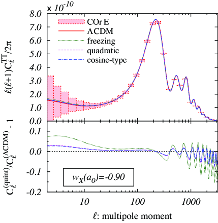
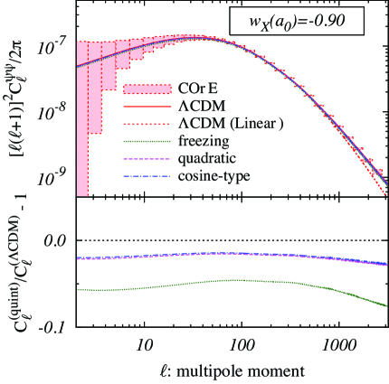
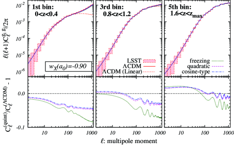
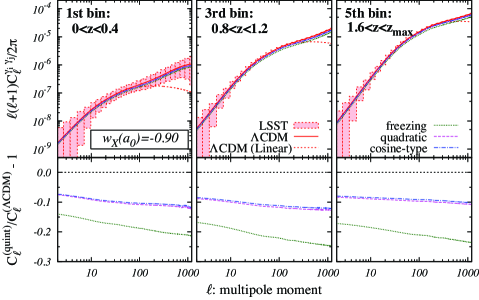
We plot angular power spectra of CMB (temperature mode and lensing potential), galaxy clustering, and galaxy weak lensing shear in Figures 1, 2 and 3, respectively. Cases for $\Lambda$CDM, freezing and thawing models are shown and both quadratic and cosine-type potential models are adopted for thawing models. Model parameters for quintessence are chosen such that the present value of the equation of state becomes $w_{X}=-0.90$. Other cosmological parameters are taken be those of the mean values of WMAP7+BAO+$H_{0}$ analysis for $\Lambda$CDM model [50]. In an analogous fashion, we show the spectra of galaxy clustering and galaxy weak lensing shear in Figure 2 and 3, respectively. Auto-correlations in the 1st, 3rd and 5th bins are only depicted for reference.

To discuss the advantage of combining multiple observational data, we consider the following two cases:

• Case I: CMB + SNe

  ${\bm{C}}_{\ell}^{XY}=\{C_{\ell}^{TT},C_{\ell}^{EE},C_{\ell}^{TE},C_{\ell}^{\psi\psi},C_{\ell}^{T\psi}\},$

• Case II: (CMB $\times$ Galaxy clustering $\times$ Galaxy weak lensing) + SNe

  ${\bm{C}}_{\ell}^{XY}=\{C_{\ell}^{TT},C_{\ell}^{EE},C_{\ell}^{TE},C_{\ell}^{\psi\psi},C_{\ell}^{T\psi},C_{\ell}^{{\rm g}_{i}{\rm g}_{j}},C_{\ell}^{{\gamma}_{i}{\gamma}_{j}},C_{\ell}^{{\rm g}_{i}{\gamma}_{j}},C_{\ell}^{T{\rm g}_{i}},C_{\ell}^{T{\gamma}_{i}},C_{\ell}^{\psi{\rm g}_{i}},C_{\ell}^{\psi{\gamma}_{i}},\},$

where Case I corresponds to the constraint from CMB, and Case II corresponds to that from auto-correlations of CMB, galaxy clustering and galaxy weak lensing with cross-correlations between different surveys. Both cases include the information from the SNe survey, for which we assume JDEM-like specification.

Then we define the total chi-square of all observables $\chi^{2}_{\rm tot}$ as

$$\chi^{2}_{\rm tot}=\chi^{2}_{\rm(I\,or\,II)}({\bm{C}_{\ell,\,{\rm mod}}})+\chi^{2}_{\rm SNe}({\bm{\mu}_{i,\,{\rm mod}}}),$$ (48)

where $\chi^{2}_{\rm(I\,or\,II)}({\bm{C}_{\ell,\,{\rm mod}}})$ denotes the chi-square for the angular power spectra given in Eq. (42) for Case I or Case II, respectively, and $\chi^{2}_{\rm SNe}({\bm{\mu}_{i,\,{\rm mod}}})$ is that from the SNe survey (given by Eq. (53) in Appendix A.3).

Figure 2: Same as Figure 1 except for the angular power spectra of the galaxy clustering. The filled boxes are binning noise spectrum for the LSST survey. We plot only the auto-correlations ones for the 1st, 3rd and 5th bins in the figure.

Figure 3: Same as Figure 2 but for the angular power spectra of the galaxy weak lensing shear.

We explore the parameter space by Markov-chain Monte-Carlo method and for this purpose we modify the publicly available code CosmoMC [40]. To estimate the constraints, we adopt the range of multipole moments as [$\ell_{\rm min}$,$\ell_{\rm max}$]=[2,2000] for CMB observables ($T$,$E$,$\psi$), and [$\ell_{\rm min}$,$\ell_{\rm max}$]=[2,200] for the LSS observables (${\rm g}$,$\gamma$), respectively. For the cross-correlations between CMB and LSS observables, we adopt the same range as that for LSS.

5 Forecast

Now we discuss the possibility to distinguish the different quintessence models which give the same present value of $w_{X}$ from future cosmological surveys. For this purpose, we derive the constraints for parameterized dark energy models described in Section 3.2 using the mock data generated by assuming the three fiducial quintessence models. The first fiducial model is the thawing model in which the potential is a simple quadratic potential given by Eq. (8) and labeled as “Thawing I.” The second one is the thawing model with the potential of a cosine-type given by Eq. (9) and labeled as “Thawing II.” The final one is the freezing model in which the potential is a typical inverse power-law type given by Eq. (10) and labeled as “Freezing”. As for the parameterizations of the dark energy equation of state, we adopt the three parameterizations given by Eqs. (11), (13), and (26).

Since perturbation equations are unstable for dark energy models crossing $w_{X}=-1$, we introduce a prior for dark energy equation of state which forbids the crossing of $w_{X}=-1$. We note that this is a reasonable assumption for this work because quintessence models with the canonical kinetic term predict its equation of state to be $w_{X}\geq-1$. However, to check this prior effect, we compare the models with or without the prior for “Parameterization I” in Appendix A.4 by using only the background quantities.

Figure 4: Expected constraints for Parameterization I from SNe + CMB (left) and SNe + CMB + LSS (right). The present value of the equation of state for each fiducial model is chosen as $w_{X}(a_{0})=-0.90$ (top) and $w_{X}(a_{0})=-0.95$ (bottom), respectively. The contours show the 68% and 95% confidence level for Freezing (green), Thawing I (magenta), and Thawing II (cyan).

Now we investigate how much we can differentiate the thawing and the freezing models from future observations of CMB, galaxy clustering and weak lensing shear. In the analysis, we vary standard six cosmological parameters plus the model parameters of the dark energy equation of state $w_{X}(a)$ for each parameterization and the galaxy bias parameter $b_{\rm g}(z)$;

$$\{\Omega_{\rm b}h^{2},~{}\Omega_{\rm c}h^{2},~{}\theta_{\rm s},~{}\tau^{\rm reion},~{}n_{\rm s},~{}A_{\rm s}~{}\}+\left\{\begin{array}[]{c}{\rm model~{}parameters~{}of~{}}w_{X}(a)\end{array}\right\}+\left\{{\rm galaxy~{}bias}~{}b_{\rm g}(z);~{}M_{\rm min}\right\}$$

where $\Omega_{\rm b}$ and $\Omega_{\rm c}$ are the density parameters of baryon and CDM, $h$ is the dimension-less Hubble parameter, $\theta_{\rm s}$ is the ratio of the sound horizon to the angular diameter distance, $\tau^{\rm reion}$ is the optical depth of reionization, $n_{\rm s}$ and $A_{\rm s}$ are the spectral index and the amplitude of the initial power spectrum, respectively. Additionally, we include the parameter $M_{\rm min}$ shown in Eq. (36) to determine the galaxy bias parameter when the observable of galaxy clustering is included.

5.1 Difference between Thawing and Freezing models

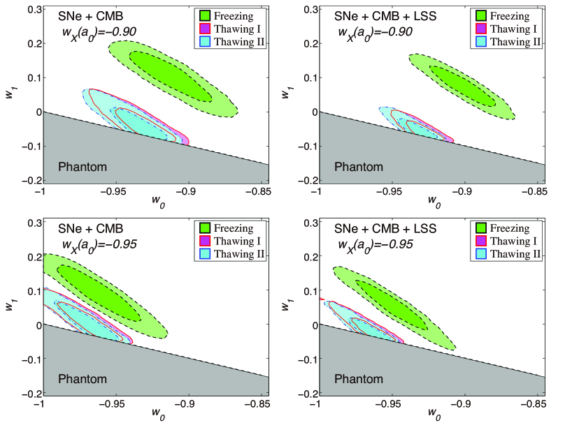
Here we show the constraints on the cosmological parameters and the parameters for the dark energy equation of state for the three fiducial models of quintessence, which are the potential models given in Sec. 2 and labeled as Thawing I, Thawing II and Freezing in the figures hereafter. In Figure 4, we adopt “Parameterization I” given in Eq. (11) and show the constraints projected on the $w_{0}-w_{1}$ plane. The fiducial models of quintessence in the top and bottom panels have different values of the equation of state at present time with $w_{X}(a_{0})=-0.90$ and $w_{X}(a_{0})=-0.95$, respectively. For other cosmological parameters, we take the mean values from WMAP7+BAO+$H_{0}$ analysis for the $\Lambda$CDM model [50] as their fiducial ones. In the figure, the gray region corresponds to so-called phantom one with $w_{0}+w_{1}<-1$, which is excluded by the prior mentioned above. The best-fit values and derived mean values with marginalized 1-$\sigma$ errors for the parameters of Parameterization I are summarized in Table 3.

We can find clear difference between the thawing and the freezing models on these planes even without the LSS observables. However, for our purpose to discriminate them, the sign of $w_{1}$ is crucially important because $w_{1}<0$ is expected for the thawing models and $w_{1}>0$ for the freezing ones. From this viewpoint, we can conclude that, only for the case with $w_{X}(a_{0})=-0.90$, they can be discerned at $1\sigma$ confidence level (CL) without the LSS observables. The LSS observables can further improve the constraint and enables us to discriminate them at more than $1\sigma$ ($2\sigma$) CL as long as the present equation of state $w_{X}(a_{0})\hskip 3.00003pt\raisebox{1.72218pt}{$>$}\raisebox{-3.01385pt}{$\sim$}\hskip 1.00006pt-0.95~{}(-0.90)$.

	$w_{0}$			$w_{1}$
	Best fit	68% limits		Best fit	68% limits	$\chi_{\rm min}^{2}$
$w_{X}(a_{0})=-0.90$
Freezing
SNe + CMB	-0.90	-0.91 $\pm$ 0.018		0.089	0.101 $\pm$ 0.048	3.250
SNe + CMB + LSS	-0.90	-0.90 $\pm$ 0.015		0.084	0.074 $\pm$ 0.040	6.949
Thawing I
SNe + CMB	-0.93	-0.93 $\pm$ 0.013		-0.044	-0.036 $\pm$ 0.035	3.445
SNe + CMB + LSS	-0.92	-0.93 $\pm$ 0.009		-0.076	-0.053 $\pm$ 0.022	4.467
Thawing II
SNe + CMB	-0.92	-0.94 $\pm$ 0.014		-0.075	-0.031 $\pm$ 0.036	3.652
SNe + CMB + LSS	-0.93	-0.94 $\pm$ 0.009		-0.062	-0.047 $\pm$ 0.023	4.921
$w_{X}(a_{0})=-0.95$
Freezing
SNe + CMB	-0.96	-0.96 $\pm$ 0.018		0.079	0.086 $\pm$ 0.052	3.302
SNe + CMB + LSS	-0.94	-0.95 $\pm$ 0.017		0.037	0.052 $\pm$ 0.048	4.404
Thawing I
SNe + CMB	-0.96	-0.97 $\pm$ 0.013		-0.020	0.006 $\pm$ 0.036	3.438
SNe + CMB + LSS	-0.96	-0.97 $\pm$ 0.010		-0.041	-0.013 $\pm$ 0.027	4.133
Thawing II
SNe + CMB	-0.96	-0.97 $\pm$ 0.013		-0.010	0.008 $\pm$ 0.036	3.410
SNe + CMB + LSS	-0.96	-0.97 $\pm$ 0.010		-0.040	-0.011 $\pm$ 0.025	4.209

Table 3: Best-fit values and 68% confidence limits for Parameterization I.

Figure 5: Same as Figure 4, except for the constraints for Parameterization II with the value of $q=0.8$.

Figure 6: Same as Figure 4, except for the constraints for Parameterization II with the value of $q=100$.

	$w_{a}$			$w_{b}$			$a_{s}$
	Best fit	68% limits		Best fit	68% limits		Best fit	68% limits	$\chi_{\rm min}^{2}$
$w_{X}(a_{0})=-0.90~{}(q=0.8)$
Freezing
SNe + CMB	-0.99	-0.94 $\pm$ 0.039		-0.75	-0.81 $\pm$ 0.036		0.38	0.60 $\pm$ 0.19	3.479
SNe + CMB + LSS	-0.98	-0.93 $\pm$ 0.038		-0.77	-0.83 $\pm$ 0.028		0.42	0.63 $\pm$ 0.18	6.322
Thawing I
SNe + CMB	-0.91	-0.93 $\pm$ 0.029		-0.98	-0.95 $\pm$ 0.029		0.67	0.67 $\pm$ 0.19	3.619
SNe + CMB + LSS	-0.91	-0.92 $\pm$ 0.024		-0.99	-0.97 $\pm$ 0.022		0.55	0.69 $\pm$ 0.19	6.056
Thawing II
SNe + CMB	-0.91	-0.94 $\pm$ 0.028		-0.99	-0.96 $\pm$ 0.027		0.55	0.68 $\pm$ 0.19	3.710
SNe + CMB + LSS	-0.90	-0.93 $\pm$ 0.024		-0.99	-0.97 $\pm$ 0.022		0.88	0.70 $\pm$ 0.19	6.003
$w_{X}(a_{0})=-0.95~{}(q=0.8)$
Freezing
SNe + CMB	-0.99	-0.96 $\pm$ 0.032		-0.87	-0.90 $\pm$ 0.034		0.57	0.62 $\pm$ 0.19	3.973
SNe + CMB + LSS	-0.99	-0.95 $\pm$ 0.033		-0.86	-0.91 $\pm$ 0.034		0.47	0.64 $\pm$ 0.19	4.110
Thawing I
SNe + CMB	-0.95	-0.97 $\pm$ 0.020		-0.98	-0.96 $\pm$ 0.020		0.93	0.66 $\pm$ 0.19	3.284
SNe + CMB + LSS	-0.98	-0.97 $\pm$ 0.018		-0.96	-0.97 $\pm$ 0.018		0.85	0.66 $\pm$ 0.19	4.772
Thawing II
SNe + CMB	-0.97	-0.97 $\pm$ 0.019		-0.96	-0.96 $\pm$ 0.019		0.70	0.66 $\pm$ 0.19	3.357
SNe + CMB + LSS	-0.96	-0.97 $\pm$ 0.017		-0.98	-0.97 $\pm$ 0.017		0.64	0.67 $\pm$ 0.19	4.700
$\bm{w_{X}(a_{0})=-0.90~{}(q=100)}$
Freezing
SNe + CMB	-0.89	-0.90 $\pm$ 0.039		-0.85	-0.84 $\pm$ 0.039		0.66	0.64 $\pm$ 0.21	2.874
SNe + CMB + LSS	-0.89	-0.89 $\pm$ 0.029		-0.85	-0.84 $\pm$ 0.026		0.57	0.64 $\pm$ 0.20	6.150
Thawing I
SNe + CMB	-0.92	-0.90 $\pm$ 0.056		-0.96	-0.96 $\pm$ 0.017		0.73	0.74 $\pm$ 0.19	3.029
SNe + CMB + LSS	-0.90	-0.90 $\pm$ 0.060		-0.96	-0.97 $\pm$ 0.012		0.77	0.79 $\pm$ 0.12	3.868
Thawing II
SNe + CMB	-0.91	-0.89 $\pm$ 0.065		-0.96	-0.96 $\pm$ 0.016		0.82	0.76 $\pm$ 0.19	3.111
SNe + CMB + LSS	-0.90	-0.88 $\pm$ 0.063		-0.97	-0.97 $\pm$ 0.011		0.80	0.79 $\pm$ 0.14	3.885
$\bm{w_{X}(a_{0})=-0.95~{}(q=100)}$
Freezing
SNe + CMB	-0.94	-0.94 $\pm$ 0.036		-0.88	-0.90 $\pm$ 0.046		0.44	0.61 $\pm$ 0.21	3.025
SNe + CMB + LSS	-0.94	-0.93 $\pm$ 0.042		-0.91	-0.91 $\pm$ 0.034		0.56	0.63 $\pm$ 0.22	4.114
Thawing I
SNe + CMB	-0.87	-0.92 $\pm$ 0.072		-0.97	-0.97 $\pm$ 0.016		0.95	0.76 $\pm$ 0.21	3.090
SNe + CMB + LSS	-0.94	-0.91 $\pm$ 0.072		-0.98	-0.97 $\pm$ 0.025		0.86	0.75 $\pm$ 0.20	3.914
Thawing II
SNe + CMB	-0.91	-0.92 $\pm$ 0.072		-0.97	-0.97 $\pm$ 0.013		0.94	0.77 $\pm$ 0.20	3.126
SNe + CMB + LSS	-0.95	-0.91 $\pm$ 0.071		-0.98	-0.98 $\pm$ 0.012		0.86	0.79 $\pm$ 0.19	3.852

Table 4: Best-fit values and 68% confidence limits for Parameterization II.

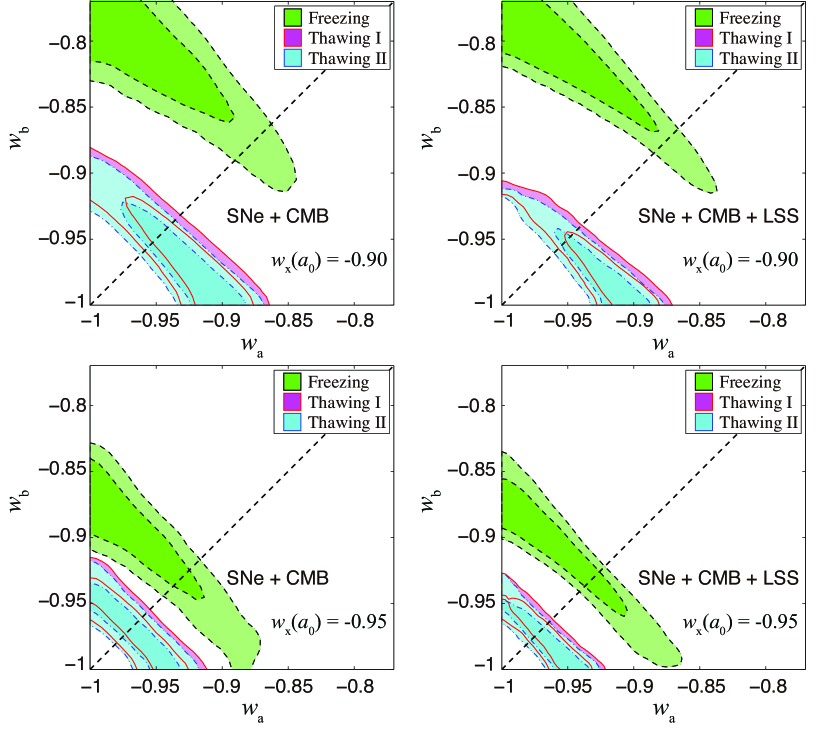
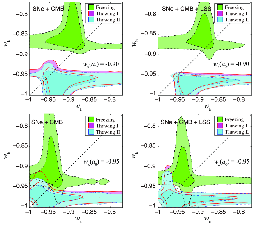
We also study constraints adopting another parameterization for the equation of state to see its dependence on the parameterization. In Figure 5 and 6, we show the results for “Parameterization II” given by Eq. (13). Although this parameterization contains four parameters $w_{a}$, $w_{b}$, $a_{s}$ and $q$, we fix the value of $q$ as $0.8$ and $100$ for Figure 5 and 6, respectively. The different values of $q$ give the different slope or interval of the evolution for the dark energy equation of state. Small $q$ gives a mild and long-term shift of $w_{X}(a)$ while large $q$ gives a rapid and short-term shift. The figures represent constraints on the $w_{a}-w_{b}$ plane. For the same reason as discussed above, we prohibit the phantom region of dark energy equation of state with $w_{X}(a)<-1$, which corresponds to $w_{a}<-1$ and $w_{b}<-1$ in this parameterization. The best-fit values and derived mean values with marginalized 1$\sigma$ errors for the parameters of Parameterization II are summarized in Table 4.

In the case of $q=0.8$, the thawing and the freezing models show up in different parameter regions even without the LSS observables. Note, however, that the allowed region should appear in the down-right side ($w_{a}>w_{b}$) on the $w_{a}-w_{b}$ plane for thawing models while in the up-left side ($w_{b}>w_{a}$) for freezing ones. In this respect, we conclude from Figure 5 that we cannot distinguish them without the LSS observables. Only when combing the LSS observables, they can be differentiated at $1\sigma$ CL only for the case with $w_{X}(a_{0})=-0.90$. For the case with $w_{X}(a_{0})=-0.95$, we cannot make a definite statement for the difference between the thawing and the freezing models.

Let us move on to the case of $q=100$. Apparently, the distributions of allowed regions drastically change (Figure 6). This is because the evolution of the equation of state shows an instantaneous transition and the constraints are almost determined by the value of equation of state in the fiducial model at the present epoch. If the transition of the equation of state occurs early enough, it is almost constant, $w_{X}(a)\simeq w_{a}$, over the observationally relevant epoch. However, the results are almost the same as those for the case of $q=0.8$ in terms of discrimination of the thawing and the freezing models. As shown in Figure 6, they can be distinguished at $1\sigma$ CL only for the case with $w_{X}(a_{0})=-0.90$ while they are indistinguishable for the case with $w_{X}(a_{0})=-0.95$.

To summarize, as for parameterization II, there is no substantial difference between the cases with $q=0.8$ and $q=100$ in order to distinguish between the thawing and the freezing models on the $w_{a}-w_{b}$ plane.

Figure 7: Same as Figure 4, but for the constraints for Parameterization III.

5.2 The sign of the effective mass squared within thawing models

In this subsection, we investigate the possibility of distinguishing the different thawing quintessence models, i.e., quadratic and cosine-type potentials. For this purpose, we focus on the sign of the effective mass squared of the potentials and adopt Parameterization III given in Eq. (26).

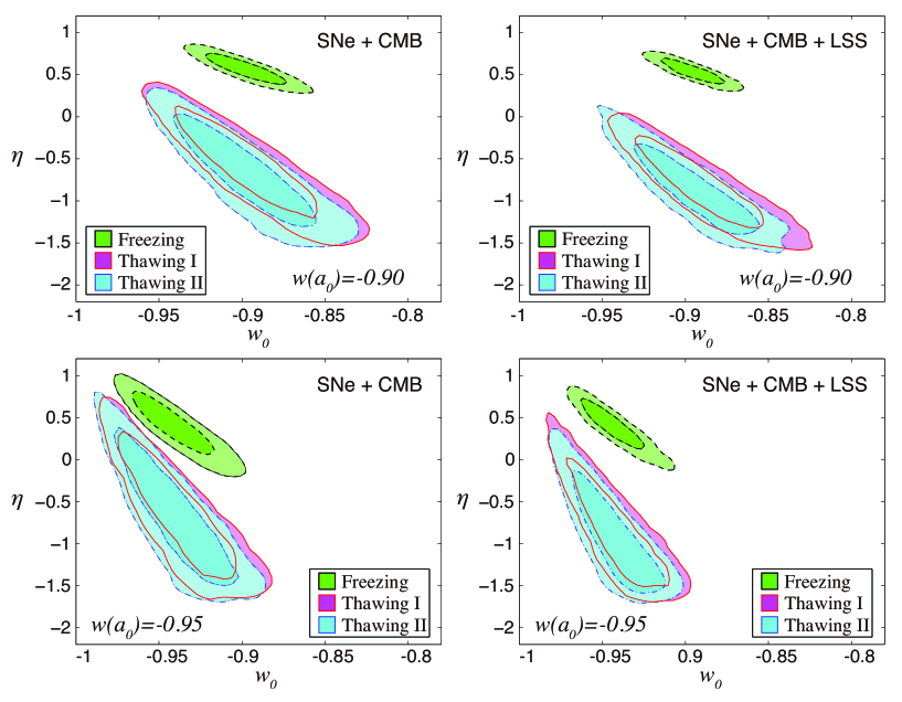
In Figure 7, we show the results for Parameterization III. While the main purpose of this analysis is to investigate whether we can differentiate the sign of the effective mass of the potential for the thawing model, we also show the constraint on the freezing model in the same figures for comparison. The best-fit values and derived mean values with marginalized 1$\sigma$ errors for the parameters of Parameterization III are summarized in Table 5.

Despite our expectation, constraints on the parameter $\eta$ are indistinguishable within the thawing models, i.e., quadratic and cosine-type potentials. This is because the parameter $\eta$ not only serves as potential curvature but also affects the time evolution of the equation of state. In other words, the information about $\eta$ is obtained mainly through Eq. (25) and not through Eq. (24). Even if we combine the LSS observables, we cannot see the difference of the effective mass squared between the two thawing models.

	$w_{0}$			$\eta$
	Best fit	68% limits		Best fit	68% limits	$\chi_{\rm min}^{2}$
$w_{X}(a_{0})=-0.90$
Freezing
SNe + CMB	-0.90	-0.90 $\pm$ 0.015		-0.57	-0.55 $\pm$ 0.12	2.902
SNe + CMB + LSS	-0.90	-0.90 $\pm$ 0.012		-0.59	-0.54 $\pm$ 0.10	7.108
Thawing I
SNe + CMB	-0.91	-0.89 $\pm$ 0.028		0.39	0.60 $\pm$ 0.41	3.152
SNe + CMB + LSS	-0.90	-0.89 $\pm$ 0.025		0.70	0.83 $\pm$ 0.34	4.257
Thawing II
SNe + CMB	-0.91	-0.90 $\pm$ 0.027		0.40	0.68 $\pm$ 0.41	3.202
SNe + CMB + LSS	-0.88	-0.90 $\pm$ 0.025		1.11	1.06 $\pm$ 0.34	4.570
$w_{X}(a_{0})=-0.95$
Freezing
SNe + CMB	-0.95	-0.94 $\pm$ 0.016		-0.57	-0.41 $\pm$ 0.24	3.241
SNe + CMB + LSS	-0.95	-0.94 $\pm$ 0.013		-0.39	-0.40 $\pm$ 0.20	4.646
Thawing I
SNe + CMB	-0.95	-0.94 $\pm$ 0.022		0.37	0.63 $\pm$ 0.52	3.284
SNe + CMB + LSS	-0.95	-0.94 $\pm$ 0.019		0.71	0.84 $\pm$ 0.48	4.116
Thawing II
SNe + CMB	-0.95	-0.95 $\pm$ 0.029		0.42	0.30 $\pm$ 0.99	3.169
SNe + CMB + LSS	-0.93	-0.94 $\pm$ 0.017		1.08	0.92 $\pm$ 0.46	4.017

Table 5: Best-fit values and 68% confidence limits for Parameterization III.

5.3 Discussion

We performed analyses assuming some parameterizations for the dark energy equation of state. Constraints on each parameter plane depend on the parameterization, and the degree of how we can distinguish the different potential models also varies by the parameterizations. Here we discuss what parameterization of the dark energy equation of state we should adopt in order to discriminate quintessence models.

As shown in the previous section, Parameterization I enables us to discriminate them at more than $1\sigma$ ($2\sigma$) CL for the present equation of state $w_{X}(a_{0})\hskip 3.00003pt\raisebox{1.72218pt}{$>$}\raisebox{-3.01385pt}{$\sim$}\hskip 1.00006pt-0.95~{}(-0.90)$. On the other hand, in terms of Parameterization II with $q=0.8$ or $q=100$, they can be distinguished at $1\sigma$ CL only for the case with $w_{X}(a_{0})=-0.90$ while they are indistinguishable for the case with $w_{X}(a_{0})=-0.95$. In the analysis, we fixed the parameter $q$ (albeit varied $a_{s}$) simply because we need enormous numerical efforts due to the degeneracies in the parameters $q$ and $a_{s}$. However, we would expect that, if we vary both $q$ and $a_{s}$ simultaneously, the degeneracy between these parameters would in turn give another degeneracy in other parameters such as $w_{a}$ and $w_{b}$ and loosen the constraints. Therefore, for the purpose of distinguishing the thawing and the freezing models, our analysis suggests that Parameterization I would be more suitable compared to Parameterization II.

For the different potentials within the thawing model, we cannot see the apparent distinction between them from the results with the parameterizations considered in this paper. The equations of state of these two thawing models predict almost the same time evolution, however they have enormously different feature in the parameter $\eta$ given in Eq. (23). The parameter $\eta$ corresponds to the curvature of the effective mass squared of potential and those of Thawing I and Thawing II have opposite signs. To focus on these aspects, we have adopted Parameterization III and have expected that the parameter $\eta$ of this parameterization could reflect the difference between these two models effectively. However, contrary to the fact that Thawing I has a positive sign and Thawing II has a negative sign of $\eta$, the difference appears only between thawing ($\eta<0$) and freezing ($\eta>0$). Absolutely, the effects on the density perturbations due to the differences of the potential’s curvature are reflected through Eq. (24), but the constraints seem to reflect the evolution of the equation of state only. Parameterization III cannot necessarily well capture the differences of curvature and we may have to consider another parameterization which can trace the property of potential more efficiently to distinguish the different potentials within the thawing models.

Now several comments on the benefits from large-scale structure surveys are in order. The different potentials of quintessence models modify the evolution of density fluctuations besides the expansion rate of the Universe. Although the temperature fluctuations of CMB can be affected by the density fluctuations of dark energy at late times through the late-ISW effect, we cannot expect large signal-to-noise ratio from this effect due to the cosmic variance. On the other hand, observables from large-scale structure surveys such as galaxy clustering and galaxy weak lensing directly trace the evolution at low redshifts where dark energy becomes the dominant component of the Universe, thus in general, we can extract the information about the evolution of the density fluctuations more effectively with LSS surveys. Furthermore, the observable from the SNe survey provides only the information of background quantities through distance measurement. Actually the information from the SNe survey plays the most dominant role in the constraint of the equation of state parameters, but the information about density fluctuations is independent and helps to break the degeneracies among model parameters. Additionally, the different potentials of the thawing models show a similar evolution of the equation of state and the difference between them appears in the evolution of density fluctuations. Therefore, the information about the density fluctuations is absolutely necessary to distinguish the potential models more finely.

In fact, although the inclusion of LSS data has not drastically improved the constraints on dark energy parameters in our analysis, such improvement is useful to discriminate the thawing and the freezing models, as discussed in the subsection 5.1. For example, in the case of Parameterization I, we can differentiate the models at $1\sigma$ confidence level (CL) without the LSS observables only for the case with $w_{X}(a_{0})=-0.90$. However, the inclusion of the LSS observables enables us to discriminate them at more than $1\sigma$ ($2\sigma$) CL as long as the present equation of state $w_{X}(a_{0})\hskip 3.00003pt\raisebox{1.72218pt}{$>$}\raisebox{-3.01385pt}{$\sim$}\hskip 1.00006pt-0.95~{}(-0.90)$. We should also note that there is a possibility of putting tighter constraints on dark energy from future survey of LSS such as Euclid [43]. Euclid is a satellite telescope and provides spectroscopic redshift information. The spectroscopic redshift survey provides more information than photometric redshift surveys and allows us to measure the three-dimensional galaxy power spectra. Therefore, the spectroscopic survey by Euclid will have a potential to put tighter constraints on dark energy, which will be a next step of this work.

On the other hand, constraints from the LSS observables can be affected by the designs of survey, for example observing redshift range, the number or width of redshift bins, systematics of surveys, and so on. One of the most serious theoretical uncertainties of LSS survey is the non-linearity of matter power spectra on small scales. In such scales, we have to take care of mode-couplings for the estimation of covariance matrix and the misestimation may lead to an incorrect constraint. However we used the information only in relatively large scale region where the linear theory is reasonably satisfied for the observables of the galaxy clustering and galaxy weak lensing. Therefore, the systematics due to the non-linearity should be small in our analysis, and the covariance matrix used in this paper would give a reasonable estimate. In addition to the above uncertainties, there are various systematics for galaxy weak lensing shear survey, for example, on the measurement of galaxy shear and the uncertainties due to photometric redshift measurement. They make crucial systematics for constraints on dark energy and/or other parameters [44, 45]. In this paper, we take into account those systematics as the uncertainties of the observables. Therefore, the effects from the other systematics should not affect our results much.

6 Summary

We performed the analysis to investigate how we can distinguish the different models of quintessence from cosmological surveys in a next few decades. In this paper we adopted three types of quintessence potentials as the fiducial models and explored the cosmological parameter space with MCMC method for each fiducial model. For fitting models, we assumed some parameterizations for the dark energy equation of state, and considered future cosmological surveys such as those of the type-Ia supernovae (JDEM), CMB (COrE) and large scale structures (LSST).

Regarding the differentiations of the thawing and the freezing quintessence models, we can discriminate them at more than $1\sigma$ ($2\sigma$) CL for the case with the present equation of state $w_{X}(a_{0})\hskip 3.00003pt\raisebox{1.72218pt}{$>$}\raisebox{-3.01385pt}{$\sim$}\hskip 1.00006pt-0.95~{}(-0.90)$, when we make use of Parameterization I. On the other hand, weaker constraint is obtained for Parameterization II for fixed $q$’s. They can be distinguished at $1\sigma$ CL only for the case with $w_{X}(a_{0})=-0.90$ while they are indistinguishable for the case with $w_{X}(a_{0})=-0.95$. Thus, we conclude that Parameterization I would be more suitable, compared Parameterization II, in order to distinguish the thawing and the freezing quintessence models.

For further discrimination of thawing quintessence models, we considered quadratic and cosine-type potentials. In the analysis using parameterization I and II, we could not see clear differences between them. Then we considered the parameterization III which is focused on the curvature or the sign of the effective mass squared of the potential. Unfortunately, again we could not see clear differences even with this parameterization. Contrary to our expectation, it is found that this parameterization can not reflect the curvature of potentials effectively and the sign of curvature is not imprinted into the model parameters. Therefore, we conclude that we have to invent a new way of parameterization which can express the difference of potential’s curvature more effectively to distinguish the potentials of thawing models.

In this work, we concentrated on constraints on dark energy but we can apply the method here to other subjects, for example the test of gravity, neutrinos, warm dark matter models, and so on, to compare the constraints on different models. Moreover the spectroscopic surveys of large scale structure will provide more information and put tighter constraints. However, distinguishing quintessence potentials within the thawing models will not be improved by including spectroscopic surveys because a crucial problem seems to be in the parameterization of the equation of state, which will be a subject of a future work.

Appendix A Analysis with background quantities

Here we present future constraints for the quintessence models discussed in the main text only by using the information on the background evolution. One of the merits to perform such an analysis lies in the fact that we can study the effects of a prior forbidding the phantom-crossing region. To obtain the constraints from background quantities, we use projected data from COrE [38] for CMB, and JDEM [46] for SNe, and bigBOSS [47] for BAO, respectively.

A.1 CMB

For the purpose to estimate the confidence limit of each parameter only from background quantities, it is useful to introduce some parameters characterizing the CMB spectra following the method in [48]. In this way we can evaluate the confidence limit of each parameter without calculating the angular power spectra of CMB directly.

Here, we use two parameters effectively describing the information contained in the CMB spectrum, which are proposed in [48]:

$$R \equiv \sqrt{\Omega_{\rm m}H_{0}^{2}}r(z_{\rm CMB}),$$ (49)

$$\ell_{\rm a} \equiv \pi r(z_{\rm CMB})/r_{\rm s}(z_{\rm CMB}),$$ (50)

where $\Omega_{\rm m}$ and $H_{0}$ are the matter density parameter and the Hubble parameter at present time, $r(z_{\rm CMB})$ is the comoving distance from observer to the redshift of decoupling $z_{\rm CMB}$, and $r_{\rm s}(z_{\rm CMB})$ is the sound horizon at the decoupling. We calculate the redshift of decoupling via the fitting formula given in [49].

We estimate the 4$\times$4 covariance matrix for $R,~{}\ell_{a},~{}\Omega_{\rm b}h^{2}~{}{\rm and}~{}n_{\rm s}$; $\Omega_{\rm b}$ is the baryon density parameter, $h$ is the normalized Hubble parameter, and $n_{s}$ is the spectral index for the primordial power spectrum, from mock COrE data, which is composed of the temperature, polarization and CMB lensing potential angular power spectra. We adopt the specification of the CMB experiment following the COrE white paper[38], and we select the mean values of WMAP7+BAO+$H_{0}$ analysis for $\Lambda$CDM model [50] as a fiducial model of mock data. In Table 6, we show the mean values and their r.m.s (Top) and the normalized covariance matrix for $R,~{}\ell_{a},~{}\Omega_{\rm b}h^{2}~{}{\rm and}~{}n_{\rm s}$ (Bottom), which are estimated from our mock data for COrE, respectively.

Compared to the results of the Planck satellite given in [48], we find that the correlation between $\Omega_{\rm b}h^{2}$ and $\ell_{a}$ is reduced. This is not only because COrE data provide significantly tighter constraints, but attributable to our setup of analysis. The damping of temperature fluctuations on small-scale depends on $\Omega_{\rm b}h^{2}$, but the effects on this scale degenerate with other cosmological parameters such as the primordial helium mass fraction $Y_{p}$. In our analysis, we do not treat $Y_{p}$ as a free parameter, and determine the value of $Y_{p}$ from baryon density parameter $\Omega_{\rm b}h^{2}$ because $Y_{p}$ can be predicted from Big Bang Nucleosynthesis as a function of baryon and radiation densities[51]. Therefore, the high-quality data on small scales by COrE have potential to put tighter constraint on $\Omega_{\rm b}h^{2}$.

The mean value and their r.m.s variance

Parameter	Mean value	r.m.s variance
$R$	1.734	0.001617
$\ell_{a}$	302.1	0.02274
$\Omega_{\rm b}h^{2}$	0.02250	0.00005095
$n_{\rm s}$	0.9615	0.001898

The normalized covariance matrix

	$R$	$\ell_{a}$	$\Omega_{\rm b}h^{2}$	$n_{\rm s}$
$R$	1.000000	0.418460	-0.347250	-0.542950
$\ell_{a}$	0.418460	1.000000	-0.025810	-0.308290
$\Omega_{\rm b}h^{2}$	-0.347250	-0.025810	1.000000	-0.196580
$n_{\rm s}$	-0.542950	-0.308290	-0.196580	1.000000

Table 6: The mean values and rms variances for $R,~{}\ell_{a},~{}\Omega_{\rm b}h^{2},~{}n_{\rm s}$ (Top) and their covariance matrix (Bottom), which are estimated from the mock COrE data.

A.2 BAO

Baryon acoustic oscillation (BAO) can be used as a geometrical measure of the cosmic expansion, which can constrain the nature of dark energy. Its characteristic scale is set by the sound horizon, which is the distance traveled by the acoustic waves in baryon-photon plasma by the time of recombination. Such characteristic scale can be measured oriented along the line-of-sight and in its transverse direction, which can probe the Hubble parameter and the angular diameter distance, respectively. Thus we make use of the following quantities as a geometrical measure:

$$x_{1}=\frac{d_{A}(z)}{r_{s}},\qquad x_{2}=H(z)r_{s}$$ (51)

where $d_{A}(z)$ is the comoving angular diameter distance and $r_{s}$ is the sound horizon at the baryon-drag epoch. $H(z)$ is the Hubble expansion rate at a redshift $z$. To obtain an expected constraint in future BAO observations, we assume predicted fractional uncertainties in the above quantities $x_{1}$ and $x_{2}$ for bigBOSS [47].

A.3 Type-Ia Supernovae

The observables from a type-Ia supernovae survey are apparent magnitudes $m_{i}$, and provide the measurements of luminosity distances $d_{L}(z_{i})$ through the distance modulus as

$$\mu(z_{i})\equiv m_{i}-M=5\log_{10}d_{L}(z_{i})+25,$$ (52)

where $M$ represents the absolute magnitude.

In the estimation using Bayesian analysis, we can use the likelihood with several simplifying assumptions for each model given as

$$\ln{\cal L}_{(\rm SNe)}\simeq\frac{1}{2}\chi^{2}_{(\rm SNe)}({\bm{\mu}_{i,{\rm mod}}})=\frac{1}{2}\sum_{i}\frac{[\mu_{{\rm fid},i}-\mu(z_{i})]^{2}}{\sigma^{2}_{i}},$$ (53)

where we assume some redshift bins and the index of summation $i$ runs through all redshift bins, and $\mu_{{\rm fid},i}$ represents the distance modulus of a fiducial model at $i$-th redshift bin and $\sigma_{i}$ is its uncertainty.

We assume a Stage IV survey as described in the Dark Energy Task Force report[46] and the statistical random error of observed apparent magnitude is described by $\sigma_{\rm D}=0.1$. If we assume only the statistical random error and there is no correlation of errors between different samples, the uncertainty of the distance modulus at $i$-th redshift bin $\sigma_{i}$ can be written as

$$\sigma_{i}=\sigma_{\rm D}/\sqrt{N_{{\rm bin},i}}~{},$$ (54)

where $N_{{\rm bin},i}$ is the number of samples at $i$-th redshift bin, and its concrete value is also given in [46].

A.4 Constraints with background quantities

Now we investigate constraints only from background quantities, and study the effects of a prior which forbids the phantom equation of state, $w_{X}(a)<-1$, with the method described above.

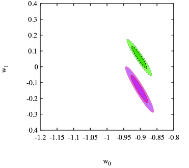
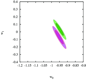
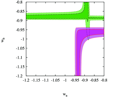
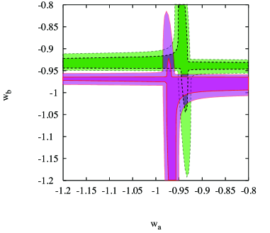
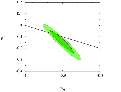
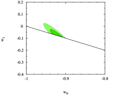
In Figures 8 and 9, we show the constraints for Parameterization I and Parameterization II, respectively, using the thawing models of the potential $V(\phi)=(1/2)m^{2}\phi^{2}$ (red/shaded) and the freezing model (green/shaded) as fiducial models.

We adopt the model parameters for the fiducial models such that the present equations of state become $w_{X}(a_{0})=-0.90$ and $w_{X}(a_{0})=-0.95$, and these values are based on the solutions of the tracker model with $\alpha=-1/3$ and $\alpha=-1/6$, respectively. The prior on the dark energy equation of state is not assumed in the figures. We find that the thawing and the freezing models can be marginally differentiated at $1\sigma$ CL for both Parameterizations as long as the present equation of state $w_{X}\simeq-0.90$, which is less constrained in comparison to the analysis done in the main text, including the information of the fluctuations.

Finally, we show the constraints from CMB (COrE), SNe (JDEM) and BAO (bigBOSS) with Parameterization I to see the effects of a prior which forbids the equation of state from crossing $w_{X}=-1$ in Figure 10. The effects of a prior do not seem sensitive to the result on these parameter spaces so much, but it shifts the center value of constraint slightly.

Figure 8: Expected constraints for Parameterization I. The fiducial models are assumed to have $V(\phi)=(1/2)m^{2}\phi^{2}$ (red/shaded) with model parameters being chosen such that the present equations of state become $w_{X}(a_{0})=-0.9$ (left) and $-0.95$ (right), and $V(\phi)=\beta M_{\rm pl}^{4}\left(\phi/M_{\rm pl}\right)^{\alpha}$ (green/shaded) with the present equations of state being $w_{X}(a_{0})=-0.9$ (left) and $-0.95$ (right), which correspond to $\alpha=-1/3$ and $-1/6$, respectively.

Figure 9: Expected constraints for Parameterization II. The fiducial models are assumed to have $V(\phi)=(1/2)m^{2}\phi^{2}$ (red/shaded) with model parameters being chosen such that the present equations of state become $w_{X}(a_{0})=-0.9$ (left) and $-0.95$ (right), and $V(\phi)=\beta M_{\rm pl}^{4}\left(\phi/M_{\rm pl}\right)^{\alpha}$ (green/shaded) with the present equations of state being $w_{X}(a_{0})=-0.9$ (left) and $-0.95$ (right), which correspond to $\alpha=-1/3$ and $-1/6$, respectively.

Figure 10: Expected constrains for Parameterization I. The fiducial model is assumed to have $V(\phi)=(1/2)m^{2}\phi^{2}$ with model parameters being chosen such that the present equation of state becomes $w_{X}(a_{0})=-0.9$. The left panel shows the result with the equation of state being allowed to enter the phantom region, $w_{X}(a)<-1$, and the right one shows the result with the phantom equation of state, $w_{X}(a)<-1$, being prohibited.

References

- [1] Y. Fujii. Phys. Rev. D 26, 2580–2588, (1982); R. D. Peccei, J. Solà, and C. Wetterich. Physics Letters B, 195, 183–190, (1987); L. H. Ford. Phys. Rev. D 35, 2339–2344, (1987); C. Wetterich. Nuclear Physics B, 302, 668–696, (1988).
- [2] B. Ratra and P. J. E. Peebles. Phys. Rev. D 37, 3406–3427, (1988); P. J. E. Peebles and B. Ratra, Astrophys. J. 325, L17 (1988).
- [3] Y. Fujii and T. Nishioka. Phys. Rev. D 42, 361–370, (1990); T. Chiba, N. Sugiyama, and T. Nakamura. MNRAS, 289, L5–L9, (1997) [astro-ph/9704199]; P. G. Ferreira and M. Joyce. Physical Review Letters, 79, 4740–4743, (1997) [astro-ph/9707286]; E. J. Copeland, A. R. Liddle, and D. Wands. Phys. Rev. D 57, 4686–4690, (1998) [gr-qc/9711068]; R. R. Caldwell, R. Dave, and P. J. Steinhardt. Physical Review Letters, 80, 1582–1585, (1998) [astro-ph/9708069].
- [4] T. Chiba, T. Okabe, and M. Yamaguchi. Phys. Rev. D 62(2), 023511, (2000) [astro-ph/9912463]; C. Armendariz-Picon, V. Mukhanov, and P. J. Steinhardt. Physical Review Letters, 85, 4438–4441, (2000) [astro-ph/0004134];
- [5] A. Kamenshchik, U. Moschella, and V. Pasquier. Physics Letters B, 511, 265–268, (2001). [gr-qc/0103004]. M. C. Bento, O. Bertolami, and A. A. Sen. Phys. Rev. D 66(4), 043507, (2002). [gr-qc/0202064].
- [6] R. R. Caldwell and E. V. Linder, Phys. Rev. Lett. 95, 141301 (2005) [astro-ph/0505494].
- [7] I. Zlatev, L. Wang, and P. J. Steinhardt. Physical Review Letters, 82, 896–899, (1999) [astro-ph/9807002]; P. J. Steinhardt, L. Wang, and I. Zlatev. Phys. Rev. D 59(12), 123504, (1999) [astro-ph/9812313].
- [8] P. Binetruy, Phys. Rev. D 60, 063502 (1999) [arXiv:hep-ph/9810553]; P. Brax and J. Martin, Phys. Lett. B 468, 40 (1999) [arXiv:astro-ph/9905040]; A. Masiero , M. Pietroni and F. Rosati, Phys. Rev. D 61, 023504 (2000) [arXiv:hep-ph/9905346]; E. J. Copeland, N. J. Nunes and F. Rosati, Phys. Rev. D 62, 123503 (2000) [arXiv:hep-ph/0005222].
- [9] J. A. Frieman, C. T. Hill, A. Stebbins, and I. Waga. Physical Review Letters, 75, 2077–2080, (1995). [astro-ph/9505060]; K. Choi. Phys. Rev. D 62(4), 043509, (2000). [hep-ph/9902292]. J. E. Kim, JHEP 0006, 016 (2000) [arXiv:hep-ph/9907528]; Y. Nomura, T. Watari and T. Yanagida, Phys. Rev. D 61, 105007 (2000) [arXiv:hep-ph/9911324]; J. E. Kim and H. P. Nilles, Phys. Lett. B 553, 1 (2003) [arXiv:hep-ph/0210402].
- [10] C. Ringeval, T. Suyama, T. Takahashi, M. Yamaguchi and S. Yokoyama, Phys. Rev. Lett. 105, 121301 (2010) [arXiv:1006.0368 [astro-ph.CO]].
- [11] C.-P. Ma and E. Bertschinger. ApJ, 455, 7, (1995). [arXiv:astro-ph/9506072].
- [12] M. Chevallier and D. Polarski, Int. J. Mod. Phys. D 10, 213 (2001) [arXiv:gr-qc/0009008].
- [13] E. V. Linder, Phys. Rev. Lett. 90, 091301 (2003) [arXiv:astro-ph/0208512].
- [14] D. Huterer and M. S. Turner, Phys. Rev. D 64, 123527 (2001) [arXiv:astro-ph/0012510].
- [15] J. Weller and A. Albrecht, Phys. Rev. D 65, 103512 (2002) [arXiv:astro-ph/0106079].
- [16] P. H. Frampton and T. Takahashi, Phys. Lett. B 557, 135 (2003) [arXiv:astro-ph/0211544].
- [17] S. Hannestad, E. Mortsell, JCAP 0409, 001 (2004). [astro-ph/0407259].
- [18] K. Ichiki and T. Takahashi. Phys. Rev. D 75(12), 123002, (2007). [arXiv:astro-ph/0703549].
- [19] W. Hu, Astrophys. J., 506, 485 (1998) [arXiv:astro-ph/9801234].
- [20] S. Ilić, M. Kunz, A. R. Liddle, and J. A. Frieman. Phys. Rev. D 81(10), 103502, (2010). [arXiv:1002.4196].
- [21] T. Chiba. Phys. Rev. D 79(8), 083517, (2009). [arXiv:0902.4037].
- [22] T. Chiba, M. Siino, and M. Yamaguchi. Phys. Rev. D 81(8), 083530, (2010). [arXiv:1002.2986].
- [23] R. Crittenden, E. Majerotto, and F. Piazza. Physical Review Letters, 98(25), 251301, (2007). [arXiv:astro-ph/0702003].
- [24] E. V. Linder. Phys. Rev. D 73(6), 063010, (2006). [arXiv:astro-ph/0601052].
- [25] R. K. Sachs and A. M. Wolfe. ApJ, 147, 73, (1967).
- [26] A. Lewis and A. Challinor. Physics Report, 429, 1–65, (2006). [arXiv:astro-ph/0601594].
- [27] W. Hu and T. Okamoto. ApJ, 574, 566–574, (2002). [arXiv:astro-ph/0111606].
- [28] T. Okamoto and W. Hu. Phys. Rev. D 67(8), 083002, (2003). [arXiv:astro-ph/0301031].
- [29] C. M. Hirata and U. Seljak. Phys. Rev. D 67(4), 043001, (2003). [arXiv:astro-ph/0209489].
- [30] A. Lewis, A. Challinor, and A. Lasenby. ApJ, 538, 473–476, (2000). [arXiv:astro-ph/9911177].
- [31] R. K. Sheth, H. J. Mo, and G. Tormen. MNRAS, 323, 1–12, (2001). [arXiv:astro-ph/9907024].
- [32] M. S. Warren, K. Abazajian, D. E. Holz, and L. Teodoro. ApJ, 646, 881–885, (2006). [arXiv:astro-ph/0506395].
- [33] M. Bartelmann and P. Schneider. Physics Report, 340, 291–472, (2001). [arXiv:astro-ph/9912508].
- [34] Z. Ma, W. Hu, and D. Huterer. ApJ, 636, 21–29, (2006). [arXiv:astro-ph/0506614].
- [35] I. Smail, R. S. Ellis, and M. J. Fitchett. MNRAS 270, 245, (1994). [arXiv:astro-ph/9402048].
- [36] A. Amara and A. Réfrégier, MNRAS 381, 1018–1026, (2007). [arXiv:astro-ph/0610127].
- [37] R. de Putter, D. Huterer, and E. V. Linder. Phys. Rev. D 81(10), 103513, (2010). [arXiv:1002.1311].
- [38] The COrE Collaboration. [arXiv:1102.2181].
- [39] LSST Science Collaborations. [arXiv:0912.0201].
- [40] A. Lewis and S. Bridle. Phys. Rev. D 66(10), 103511, (2002). [arXiv:astro-ph/0205436].
- [41] T. Chiba, A. De Felice, and S. Tsujikawa. Phys. Rev. D 87(8), 083505, (2013). [arXiv:1210.3859].
- [42] S. Dutta and R. J. Scherrer. Phys. Rev. D 78(12), 123525, (2008). [arXiv:0809.4441].
- [43] R. Laureijs, J. Amiaux, S. Arduini, J. . Auguères, J. Brinchmann, R. Cole, M. Cropper, C. Dabin, L. Duvet, A. Ealet, and et al. [arXiv:1110.3193].
- [44] D. Huterer, M. Takada, G. Bernstein, and B. Jain. MNRAS, 366, 101–114, (2006). [arXiv:astro-ph/0506030].
- [45] S. Das, R. de Putter, E. V. Linder, and R. Nakajima. ArXiv e-prints, 1102.5090, (2011). [arXiv:1102.5090].
- [46] A. Albrecht, G. Bernstein, R. Cahn, W. L. Freedman, J. Hewitt, W. Hu, J. Huth, M. Kamionkowski, E. W. Kolb, L. Knox, J. C. Mather, S. Staggs, and N. B. Suntzeff. ArXiv Astrophysics e-prints, arXiv:astro-ph/0609591, (2006). [arXiv:astro-ph/0609591].
- [47] D. Schlegel et al. [BigBoss Experiment Collaboration], arXiv:1106.1706 [astro-ph.IM].
- [48] P. Mukherjee, M. Kunz, D. Parkinson, and Y. Wang. Phys. Rev. D 78(8), 083529, (2008). [arXiv:0803.1616].
- [49] W. Hu and N. Sugiyama. ApJ, 471, 542, (1996). [arXiv:astro-ph/9510117].
- [50] E. Komatsu et al., arXiv:1001.4538 [astro-ph.CO].
- [51] J. Hamann, J. Lesgourgues, and G. Mangano. JCAP, 3, 4, (2008). [arXiv:0712.2826].
- [52] P. Mukherjee, M. Kunz, D. Parkinson, and Y. Wang. Phys. Rev. D 78(8), 083529, (2008). [arXiv:0803.1616].