$\bf L^{2}$-Error Estimates for Finite Element Approximations of Boundary Fluxes

Abstract

We prove quasi-optimal a priori error estimates for finite element approximations of boundary normal fluxes in the $L^{2}$-norm. Our results are valid for a variety of different schemes for weakly enforcing Dirichlet boundary conditions including Nitsche’s method, and Lagrange multiplier methods. The proof is based on an error representation formula that is derived by using a discrete dual problem with $L^{2}$-Dirichlet boundary data and combines a weighted discrete stability estimate for the dual problem with anisotropic interpolation estimates in the boundary zone.

1 Introduction

The normal flux at the boundary or on interior interfaces is in general of great interest in applications. Examples include surface stresses in mechanics, heat transfer through interfaces, and transport of fluid in Darcy flow.

Recently Melenk and Wohlmuth [15] has shown quasi-optimal order estimates for fluxes in a mortar setting where continuity and boundary conditions is enforced using a mortaring space of Lagrange multipliers. More precisely, they shown that the $L^{2}$-norm of the error in the normal flux is of order $|\ln h|h$ for piecewise linear polynomials and of order $h^{k}$ for piecewise polynomials of order $k$. In contrast only $h^{k-1/2}$ will be obtained if a trace inequality is used in combination with standard convergence theory for saddle point problems, see [4].

In this contribution we give an alternative proof of this result and, focusing on the case $k=1$, we also consider a wider variety of methods for weakly enforcing Dirchlet boundary conditions, including Nitsche’s method and stable and stabilized Lagrange multipliers methods.

Our proof is based on an error representation formula where the error in the normal flux is represented in terms of the interpolation error and the solution to a discrete dual problem with $L^{2}$-Dirichlet boundary data. Key to the error estimate is a stability estimate for the discrete dual problem in terms of the $L^{2}$-norm of the Dirichlet data. In the continuous case such an estimate is known, see Chabrowsky [8] and [9], and provides control of the gradient weighted with the distance to the boundary as well as a max-norm control of the $L^{2}$-norms of the solution on manifolds close to and parallel with the boundary. We prove a corresponding stability estimate for our discrete dual problem. In contrast to the approach by Melenk and Wohlmuth [15], we avoid using a Besov space framework.

Our error representation formula is related to the one derived in the Giles et al. [12], Carey et al. [7], Pehlivanov et al. [17] where various estimates for functionals of the normal flux are derived and [10] where adaptive methods based on dual problems targeting the flux in a coupled problem are developed. Note however that in our setting where we seek an a priori estimate, we employ a discrete dual problem while in the a posteriori setting, the corresponding continuous dual problem is used. Here we also establish the stability of the discrete dual problem using analytical techniques while in the duality based a posteriori error estimates, stability is often estimated using computational techniques or a known analytical stability result.

The remainder of this work is organized as follows. In Section 2 we introduce the model problem and its variational formulations we will consider throughout this work. Corresponding finite element discretizations are presented in Section 3 together with the definition of the discrete boundary fluxes. In Section 5 we prove stability bounds for the discrete dual problem and provide interpolation estimates of the solution close to the boundary. Combining these results allows us to prove $L^{2}$-error estimates for the boundary flux approximations in Section 6. In Section 7, we finally present numerical results illustrating the theoretical findings.

2 Model Problem

Let $\Omega$ be a polygonal domain in ${\mathbb{R}}^{d}$, $d=2,3$ with boundary $\partial\Omega$. We consider the elliptic model problem: find $u:\Omega\rightarrow{\mathbb{R}}$ such that

$$-\Delta u =f\quad\text{in $\Omega$}$$ (2.1)

$$u =g\quad\text{on $\partial\Omega$}$$ (2.2)

where $f$ and $g$ are given data. Then the boundary flux $\sigma_{n}$ for the solution $u$ is defined by

$$\sigma_{n}=n\cdot\nabla u$$ (2.3)

where $n$ is the outwards pointing unit normal to $\partial\Omega$.

In what follows, we consider the standard Sobolev spaces $H^{s}(U)$, $s\geqslant 0$ on some domain $U$, endowed the the usual norms $\|\cdot\|_{s,U}$ and semi-norms $|\cdot|_{s,U}$. More generally, the space $W^{s,p}(U)$ is defined as the Sobolev space consisting of all functions having $p$-integrable derivates up to order $s$ on $U$. As usual, $H^{0}(\Omega)=L^{2}(\Omega)$ and $H^{-1/2}(\partial\Omega)$ denotes the dual space of $H^{1/2}(\partial\Omega)$. Moreover, for a function $g\in H^{1/2}(\partial\Omega)$ we introduce the notation $H^{1}_{g}(\Omega)=\{v\in H^{1}(\Omega):v|_{\partial\Omega}=g\}$. The scalar product in $H^{s}(U)$ is written as $(\cdot,\cdot)_{s,U}$ and to simplify the notation, we generally omit the domain designation if $U=\Omega$ and the Sobolev index if $s=0$ in both norm and scalar product expressions. Using this notation, a weak formulation of the elliptic boundary value problem (2.1)–(2.2) is to seek $u\in H^{1}_{g}(\Omega)$ such that

$$a(u,v)=l(v)\quad\forall\,v\in H^{1}_{0}(\Omega)$$ (2.4)

where

$$a(u,v) =(\nabla u,\nabla v)$$ (2.5)

$$l(v) =(f,v)$$ (2.6)

Here, the boundary condition $u|_{\partial\Omega}=g$ is already incorporated into the trial space $H^{1}_{g}(\Omega)$. Alternatively, the boundary condition (2.2) can be enforced weakly by using a Lagrange multiplier approach. Introducing the bilinear form

$$b(\mu,v)=(\mu,v)_{\partial\Omega}$$ (2.7)

the resulting variational formulation is given by the saddle point problem: find $(u,\lambda)\in H^{1}(\Omega)\times H^{-1/2}(\partial\Omega)$ such that

$$a(u,v)+b(\lambda,v)+b(\mu,u)=l(v)+b(\mu,g)\quad\forall\,(v,\mu)\in H^{1}(\Omega)\times H^{-1/2}(\partial\Omega)$$ (2.8)

For brevity, we might denote the left-hand side by $A(u,\lambda;v,\mu)$ and the right-hand side $L(v,\mu)$. It is well-known [1, 5, 18, 22], that the saddle point problem (2.8) satisfies the Babuška-Brezzi condition, in particular

$$\sup_{v\in H^{1}(\Omega)\setminus\{0\}}\dfrac{b(\lambda,v)}{\|v\|_{1,\Omega}}\gtrsim\|\mu\|_{-1/2,\partial\Omega}\quad\forall\,\mu\in H^{-1/2}(\partial\Omega)$$ (2.9)

Consequently, problem (2.8) possesses a unique solution $(u,\lambda)$, where $u$ solves (2.1)–(2.2) in a weak sense and the Lagrange multiplier $\lambda$ represents the negative of the normal flux of $u$, i.e. $\lambda=-\sigma_{n}$.

3 Finite Element Discretizations of the Model Problem

In this section, we introduce the finite element discretizations of problem (2.1)–(2.2) we will consider throughout this work. The discretizations are defined on a quasi-uniform partition $\mathcal{T}$ of $\Omega$ into shape regular triangles in two or tetrahedra in three space dimensions with mesh parameter $h$. For a given mesh $\mathcal{T}$, let the associated finite element space of piecewise linear continuous functions be denoted by $V_{h}$. We do not assume $V_{h}\subset H^{1}_{g}(\Omega)$ and consequently, the discretizations to be considered will enforce the boundary condition (2.2) weakly. For each discretization we will define a discrete counterpart $\Sigma_{n}$ of the boundary flux (2.3).

3.1 Nitsche’s Method

The Nitsche [16] finite element method takes the form: find $u_{h}\in V_{h}$ such that

$$a_{h}(u_{h},v)=l_{h}(v)\quad\forall v\in V_{h}$$ (3.1)

where the forms are defined by

$$a_{h}(u,v) =a(u,v)-(n\cdot\nabla u,v)_{\partial\Omega}-(n\cdot\nabla u,v)_{\partial\Omega}+\beta h^{-1}(u,v)_{\partial\Omega}$$ (3.2)

$$l_{h}(v) =l(v)-(g,n\cdot\nabla v)_{\partial\Omega}+\beta h^{-1}(g,v)_{\partial\Omega}$$ (3.3)

with $\beta$ being a positive parameter. Introducing the energy norm

$$|\mspace{-1.0mu}|\mspace{-1.0mu}|v|\mspace{-1.0mu}|\mspace{-1.0mu}|^{2}=\|\nabla v\|_{\Omega}^{2}+h\|n\cdot\nabla v\|_{\partial\Omega}^{2}+h^{-1}\|v\|_{\partial\Omega}^{2}$$ (3.4)

we recall that the bilinear form $a_{h}(\cdot,\cdot)$ is continuous

$$a_{h}(u,v)\lesssim|\mspace{-1.0mu}|\mspace{-1.0mu}|u|\mspace{-1.0mu}|\mspace{-1.0mu}|\;|\mspace{-1.0mu}|\mspace{-1.0mu}|v|\mspace{-1.0mu}|\mspace{-1.0mu}|$$ (3.5)

and that if the stabilization parameter $\beta$ is large enough, a coercivity condition

$$|\mspace{-1.0mu}|\mspace{-1.0mu}|v|\mspace{-1.0mu}|\mspace{-1.0mu}|^{2}\lesssim a_{h}(v,v)\quad\forall v\in V_{h}$$ (3.6)

is satisfied, yielding the standard error estimate

$$|\mspace{-1.0mu}|\mspace{-1.0mu}|u-u_{h}|\mspace{-1.0mu}|\mspace{-1.0mu}|\lesssim h\|u\|_{2}$$ (3.7)

Here and throughout, we use the notation $a\lesssim b$ for $a\leqslant Cb$ for some generic constant $C$ which vary with the context but is always independent of the mesh size $h$. For proofs of (3.6) and (3.7), we refer to [16, 14]. To Nitsche’s method (3.1), we associate the discrete variational normal flux of the form

$$(\Sigma_{n},v)_{\partial\Omega}=(\nabla u_{h},\nabla v)_{\Omega}-(u_{h}-g,n\cdot\nabla v)_{\partial\Omega}-(f,v)_{\Omega}\quad\forall v\in V_{h}$$ (3.8)

where $\Sigma_{n}$ is the so-called Nitsche flux

$$\Sigma_{n}=n\cdot\nabla u_{h}-\beta h^{-1}(u_{h}-g)$$ (3.9)

3.2 Lagrange Multiplier Method

To formulate a finite element discretization of the saddle point problem (2.8), we assume that a discrete function space $\Lambda_{h}\subset L^{2}(\partial\Omega)\cap H^{-1/2}(\partial\Omega)$ is given, and we equip $V_{h}$, $\Lambda_{h}$ and the total approximation space $V_{h}\times\Lambda_{h}$ with the natural norms

$$|\mspace{-1.0mu}|\mspace{-1.0mu}|u|\mspace{-1.0mu}|\mspace{-1.0mu}|^{2} =\|\nabla u\|^{2}_{\Omega}+\|h^{-1/2}u\|^{2}_{\partial\Omega}$$ (3.10)

$$|\mspace{-1.0mu}|\mspace{-1.0mu}|\lambda|\mspace{-1.0mu}|\mspace{-1.0mu}|^{2} =\|h^{1/2}\lambda\|^{2}_{\partial\Omega}$$ (3.11)

$$|\mspace{-1.0mu}|\mspace{-1.0mu}|(u,\lambda)|\mspace{-1.0mu}|\mspace{-1.0mu}|^{2} =|\mspace{-1.0mu}|\mspace{-1.0mu}|u|\mspace{-1.0mu}|\mspace{-1.0mu}|^{2}+|\mspace{-1.0mu}|\mspace{-1.0mu}|\lambda|\mspace{-1.0mu}|\mspace{-1.0mu}|^{2}$$ (3.12)

respectively, see Pitkäranta [18]. Employing the discrete norms $|\mspace{-1.0mu}|\mspace{-1.0mu}|v|\mspace{-1.0mu}|\mspace{-1.0mu}|$ and $|\mspace{-1.0mu}|\mspace{-1.0mu}|\mu|\mspace{-1.0mu}|\mspace{-1.0mu}|$, it is well-known [18, 19] that the approximation space $\Lambda_{h}$ has to be designed carefully in order to satisfy the discrete equivalent of the inf-sup condition (2.9). Therefore, a stabilized Lagrange multiplier method has been proposed by Barbosa and Hughes [2, 3] where residual terms were added to circumvent the inf-sup condition (3.17). Recently, a generalized approach based on projection stabilized Lagrange multipliers has been proposed by Burman [6].

To cover a broad range of stable and stabilized Lagrange multiplier methods, we assume that the discrete saddle point problem is of the following form: find $(u_{h},\lambda_{h})\in V_{h}\times{\Lambda}_{h}$ such that

$$A_{h}(u_{h},\lambda_{h};v,\mu)=L_{h}(v,\mu)\quad\forall\,(v,\mu)\in{V}_{h}\times{\Lambda}_{h}$$ (3.13)

where

$$A_{h}(u,\lambda;v,\mu) =a(u_{h},v)+b(\lambda_{h},v)+b(\mu,u_{h})-c_{h}(u,\lambda;v,\mu)$$ (3.14)

$$L_{h}(v,\mu) =l(v)+(g,\mu)_{\partial\Omega}$$ (3.15)

Then, the approximation of the normal flux (2.3) is naturally defined by the negative of the discrete Lagrange multiplier:

$$\Sigma_{n}=-\lambda_{h}$$ (3.16)

In the variational form (3.14), the bilinear form $c_{h}(\cdot,\cdot)$ represents a consistent, possibly vanishing stabilization form such the inf-sup condition

$$\sup_{(v,\mu)\in V_{h}\times\Lambda_{h}\setminus\{(0,0)\}}\frac{A_{h}(u,\lambda;v,\mu)}{|\mspace{-1.0mu}|\mspace{-1.0mu}|(v,\mu)|\mspace{-1.0mu}|\mspace{-1.0mu}|}\gtrsim|\mspace{-1.0mu}|\mspace{-1.0mu}|(u,\lambda)|\mspace{-1.0mu}|\mspace{-1.0mu}|$$ (3.17)

holds, as well as the continuity condition

$$A_{h}(u,\lambda;v,\mu)\lesssim|\mspace{-1.0mu}|\mspace{-1.0mu}|(u,\lambda)|\mspace{-1.0mu}|\mspace{-1.0mu}|\,|\mspace{-1.0mu}|\mspace{-1.0mu}|(v,\mu)|\mspace{-1.0mu}|\mspace{-1.0mu}|$$ (3.18)

and the error estimate

$$|\mspace{-1.0mu}|\mspace{-1.0mu}|(u-u_{h},\lambda-\lambda_{h})|\mspace{-1.0mu}|\mspace{-1.0mu}|\lesssim h\|u\|_{2,\Omega}+h^{3/2}\|\lambda\|_{1,\partial\Omega}$$ (3.19)

Well-known Lagrange multiplier discretizations which are covered by these assumptions are described and analyzed in [18, 19] and [2, 3, 22]. In [18, 19], Pitkäranta proved certain local stability conditions, roughly stating that the pairing $P^{1}_{c}(\mathcal{T}_{h})\times P^{0}_{\mathrm{dc}}(\Gamma_{H})$ is stable, if the mesh size $H$ of a given discretization $\Gamma_{H}$ of the boundary $\partial\Omega=\Gamma$ satisfies the condition $h\leqslant cH$ for some $c>1$. To avoid additional meshing of the boundary and to use the natural space

$$\Lambda_{h}=\{\mu\in L^{2}(\partial\Omega)|\;\mu\in P^{0}(F)\;\forall\,F\in\partial\mathcal{T}_{h}\}$$

defined on the trace mesh $\partial\mathcal{T}$, a stabilized symmetric Lagrange Multiplier approach was proposed by Barbosa and Hughes [2, 3]. Stenberg [22] simplified the approach by showing that the weak formulation (3.13) combined with the stabilization form

$$c_{h}(u,\lambda;v,\mu)=\alpha h(\lambda+n\cdot\nabla u,\mu+n\cdot\nabla v)_{\partial\Omega}$$ (3.20)

satisfies the inf-sup condition (3.17), the continuity condition (3.18) and thus the error estimate (3.19) when $0<\alpha<C_{I}$, with $C_{I}$ being the constant in (5.11).

Finally, we would like to mention the general approach by Burman [6]. In this method, the stabilization operator is given by some symmetric form $c_{h}(\lambda,\mu)$ which, roughly speaking, controls the distance between a given discretization space $\Lambda_{h}$ and another discrete space $L_{h}$ where $V_{h}\times L_{h}$ presents an inf-sup stable pairing. Generally, the stabilization form is only required to be optimal weakly consistent and to not clutter the presentation, we skip the details for the trivial adaption of our approach to this variant.

4 Error Representation Formulas

In this section, we establish the error representation formulas for the discrete boundary fluxes. The representation formula will later allow us to bound the $L^{2}$-error of the boundary flux approximations in terms of interpolation errors and a stability estimate for the discrete solution to a suitable dual problem.

4.1 Nitsche’s Method

For given boundary data $\psi\in L^{2}(\partial\Omega)$, we define the discrete dual problem for Nitsche’s method as follows: find $\phi_{h}\in V_{h}$ such that

$$a_{h}(v,\phi_{h})=m_{\psi,h}(v)\quad\forall v\in V_{h}$$ (4.1)

where $a_{h}(\cdot,\cdot)$ is defined in (3.2) and

$$m_{\psi,h}(v)=\beta h^{-1}(\psi,v)_{\partial\Omega}-(\psi,n\cdot\nabla v)_{\partial\Omega}$$ (4.2)

Setting $v=e_{h}=\pi_{h}u-u_{h}$ we obtain

$$a_{h}(e_{h},\phi_{h})=m_{\psi,h}(e_{h})$$ (4.3)

Using Galerkin orthogonality, we note that the left hand side can be written

$$a_{h}(e_{h},\phi_{h})=a_{h}(\pi_{h}u-u,\phi_{h})$$ (4.4)

and for the right hand side

$$m_{\psi,h}(e_{h})=m_{\psi,h}(\pi_{h}u-u)+m_{\psi,h}(u-u_{h})$$ (4.5)

where the second term takes the form

$$m_{\psi,h}(u-u_{h}) =(\beta h^{-1}(u-u_{h}),\psi)-(n\cdot\nabla(u-u_{h}),\psi)_{\partial\Omega}$$ (4.6)

$$=(\beta h^{-1}(g-u_{h})+n\cdot\nabla u_{h}-n\cdot\nabla u,\psi)_{\partial\Omega}$$ (4.7)

$$=(\Sigma_{n}(u_{h})-\sigma_{n}(u),\psi)_{\partial\Omega}$$ (4.8)

Collecting these identities, we arrive at the error representation formula

$$(\sigma_{n}(u)-\Sigma_{n}(u_{h}),\psi)_{\partial\Omega}=a_{h}(u-\pi_{h}u,\phi_{h})-m_{\psi,h}(u-\pi_{h}u)$$ (4.9)

Thus we have the following

Lemma 4.1.

With $\sigma_{n}(u)$ and $\Sigma_{n}(u_{h})$ defined by (2.3) and (3.8) it holds

$$\|\sigma_{n}(u)-\Sigma_{n}(u_{h})\|_{\partial\Omega}\leqslant\sup_{\psi\in L^{2}(\partial\Omega)\setminus\{0\}}\frac{1}{\|\psi\|_{\partial\Omega}}\Big{(}|a_{h}(u-\pi_{h}u,\phi_{h})|+|m_{\psi,h}(u-\pi_{h}u)|\Big{)}$$ (4.10)

4.2 Lagrange Multiplier Method

We consider the following discrete dual problem: find $(\phi_{h},\theta_{h})\in{V}_{h}\times\Lambda_{h}$ such that

$$A_{h}(v,\mu;\phi_{h},\theta_{h})=m_{\psi,h}(\mu)\quad\forall\,(v,\mu)\in{V}_{h}\times{\Lambda}_{h}$$ (4.11)

where $A_{h}(\cdot,\cdot)$ is defined as in (3.14) and

$$m_{\psi,h}(\mu)=(\psi,\mu)_{\partial\Omega}$$ (4.12)

Setting $(v,\mu)=(\pi_{h}u-u_{h},\pi_{h}\lambda-\lambda_{h})$ and using Galerkin orthogonality, we obtain

$$m_{\psi,h}(\pi_{h}\lambda-\lambda_{h}) =A_{h}(\pi_{h}u-u_{h},\pi_{h}\lambda-\lambda_{h};\phi_{h},\theta_{h})$$

$$=A_{h}(\pi_{h}u-u,\pi_{h}\lambda-\lambda;\phi_{h},\theta_{h})$$

If we write $(\lambda-\lambda_{h},\psi)=m_{\psi,h}(\lambda-\pi_{h}\lambda)+m_{\psi,h}(\pi_{h}\lambda-\lambda_{h})$, we arrive at an error representation form similar to (4.9):

$$(\lambda-\lambda_{h},\psi)_{\partial\Omega}=A_{h}(\pi_{h}u-u,\pi_{h}\lambda-\lambda;\phi_{h},\theta_{h})-m_{\psi,h}(\lambda-\pi_{h}\lambda)$$

Consequently, the flux error $\|\sigma_{n}(u)-\Sigma_{n}(u_{h})\|_{\partial\Omega}=\|\lambda-\lambda_{h}\|_{\partial\Omega}$ can be estimated via following

Lemma 4.2.

It holds

$$\|\lambda-\lambda_{h}\|_{\partial\Omega}\leqslant\sup_{\psi\in L^{2}(\partial\Omega)\setminus\{0\}}\frac{1}{\|\psi\|_{\partial\Omega}}\Big{(}|A_{h}(\pi_{h}u-u,\pi_{h}\lambda-\lambda;\phi_{h},\theta_{h})|+|m_{\psi,h}(\lambda-\pi_{h}\lambda)|\Big{)}$$ (4.13)

5 Stability Bounds for the Discrete Dual Problem

From the error representation formula stated in Lemma 4.1 and Lemma 4.2, we note that in order to prove estimates for the flux in the $L^{2}$-norm, we need to consider stability bounds in terms of the $L^{2}$-norm of $\psi$. Chabrowski [9] proved such estimates for the corresponding continuous problem: find $\phi:\Omega\rightarrow\mathbb{R}$ such that

$$-\Delta\phi =0\quad\text{in $\Omega$}$$ (5.1)

$$u =\psi\quad\text{on $\partial\Omega$}$$ (5.2)

with $\psi\in L^{2}(\partial\Omega)$. To state the basic energy type estimate, we shall introduce some notation that will also be needed in our forthcoming developments. Let $\rho(x)=\text{dist}(x,\partial\Omega)$ be the minimal distance between $x\in\Omega$ and $\partial\Omega$ and $p(x)\in\partial\Omega$ be the point closest to $x\in\Omega$. We note that $p(x)=x+n(p(x))\rho(x)$, where $n(p(x))$ is the exterior unit normal to $\partial\Omega$ at $p(x)$, and that there is a constant $\delta_{0}>0$, only dependent on the curvature of the boundary, such that for each $x\in\Omega$ with $\rho(x)\leqslant\delta_{0}$ there is a unique $p(x)\in\partial\Omega$. Next, we define the sets

$$\Omega_{\delta}=\{x\in\Omega:\rho(x)>\delta\}$$ (5.3)

where $0\leqslant\delta\leqslant\delta_{0}$, and we note that the closest point mapping $p:\partial\Omega_{\delta}\rightarrow\partial\Omega$ is a bijection with inverse denoted by $p^{-1}_{\delta}$. Referring to [11, Lemma 14.16], we recall that that $\rho\in C^{k}(\Omega_{\delta})$ for $k\geqslant 2$ for $\delta_{0}$ chosen small enough. If we define a weighted norm $\|v\|_{\rho,\Omega}$ by

$$\|v\|^{2}_{\rho,\Omega}=\int_{\Omega}v^{2}\rho\,\mathrm{d}x$$

then Chabrowski [9] proved the following result for the continuous problem: if $\phi\in W^{1,2}_{\mathrm{loc}}$ satisfies problem (5.1)–(5.2) in the sense that

$$\|\phi\circ p^{-1}_{\delta}-\psi\|_{\partial\Omega}\rightarrow 0\quad\text{when $\delta\rightarrow 0^{+}$}$$

then

$$\|\nabla\phi\|^{2}_{\rho,\Omega}+\|\phi\|_{\rho,\Omega}^{2}+\sup_{0\leqslant\delta\leqslant\delta_{0}}\|\phi\|^{2}_{\partial\Omega_{\delta}}\lesssim\|\psi\|^{2}_{\partial\Omega}.$$

We shall now prove a corresponding estimate for the discrete dual problems (4.1) and (4.11). In order to formulate our results, we introduce the shifted weight function

$$\rho_{\delta}=\max(0,\rho-\delta),\quad{{\delta}_{h}^{\prime}}\leqslant\delta\leqslant\delta_{0}$$ (5.4)

and we let

$${{\delta}_{h}^{\prime}}=C^{\prime}h$$ (5.5)

with the constant $C^{\prime}>0$ chosen such that $\rho_{{{\delta}_{h}^{\prime}}}=0$ on all elements with a face on the boundary $\partial\Omega$, see Figure 5.2. The existence of such a constant $C^{\prime}$ follows from the assumed quasi-uniformity of the mesh. In the case where $\Omega$ is not a $C^{2}$-domain but rather a convex polyhedral domain described by faces $\{F_{i}\}_{i=1}^{N}$, we define stripes $S_{\delta}(F_{i})=\{x\in\mathbb{R}:\exists x_{0}\in F_{i}\wedge\exists t\text{ s.t. }x=x_{0}+t\cdot n\wedge 0\leqslant t\leqslant\delta\}$, cf. Figure 5.1. Then the analysis presenting in this work carries over by considering each stripe at a time and the fact that locally only a finite number of stripes overlaps.

Fig. 5.1: Polyhedral domain $\Omega$ with faces $\{F_{i}\}_{i=1}^{6}$ with corresponding stripes $S_{\delta}(F_{i})$ charted in different colors.

We state now the main result of this section.

Proposition 5.1.

Let $\phi_{h}\in V_{h}$ be the solution of the discrete dual problem (4.1). Then $\phi_{h}$ satisfies the stability estimate

$$\|\nabla\phi_{h}\|^{2}_{\rho_{{{\delta}_{h}^{\prime}}},\Omega}+h\|\nabla\phi_{h}\|^{2}_{\Omega}+\sup_{0\leqslant\delta\leqslant\delta_{0}}\|\phi_{h}\|^{2}_{\partial\Omega_{\delta}}+\|\phi_{h}\|_{\Omega}^{2}\lesssim\|\psi\|^{2}_{\partial\Omega}$$ (5.6)

Alternatively, if $(\phi_{h},\theta_{h})\in V_{h}\times\Lambda_{h}$ is the solution of the discrete dual problem (4.11), then

$$\|\nabla\phi_{h}\|^{2}_{\rho_{{\delta}_{h}^{\prime}},\Omega}+h\|\nabla\phi_{h}\|^{2}_{\Omega}+h^{2}\|\theta_{h}\|^{2}_{\partial\Omega}+\sup_{0\leqslant\delta\leqslant\delta_{0}}\|\phi_{h}\|^{2}_{\partial\Omega_{\delta}}+\|\phi_{h}\|_{\Omega}^{2}\lesssim\|\psi\|^{2}_{\partial\Omega}$$ (5.7)

Before we present the elaborated proof of Proposition 5.1 in Section 5.2, the next section collects useful inequalities and interpolation estimates which will be used throughout the remaining work.

5.1 Interpolation Error Estimates

We recall the following trace inequality for $v\in H^{1}(\Omega)$:

$$\|v\|_{\partial T} \lesssim h_{T}^{-1/2}\|v\|_{T}+h_{T}^{1/2}\|\nabla v\|_{T}\quad\forall\,T\in\mathcal{T}$$ (5.8)

$$\|v\|_{T\cap\partial\Omega} \lesssim h_{T}^{-1/2}\|v\|_{T}+h_{T}^{1/2}\|\nabla v\|_{T}\quad\forall\,T\in\mathcal{T}$$ (5.9)

See Hansbo and Hansbo [13] for a proof of (5.9). We will also need the following well-known inverse estimates for $v_{h}\in V_{h}$:

$$\|\nabla v_{h}\|_{T} \lesssim h_{T}^{-1}\|v_{h}\|_{T} \forall\,T\in\mathcal{T}$$ (5.10)

$$\|h^{1/2}n\cdot\nabla v_{h}\|_{F} \lesssim\|\nabla v_{h}\|_{T} \forall\,T\in\mathcal{T}$$ (5.11)

Let $\pi_{h}:L^{2}(\Omega)\rightarrow V_{h}$ be the standard Scott–Zhang interpolation operator [21] and recall the interpolation error estimates

$$\|v-\pi_{h}v\|_{r,T} \lesssim h^{s-r}|v|_{s,\omega(T)} \quad 0\leqslant r\leqslant s\leqslant 2\quad \forall\,T\in\mathcal{T}$$ (5.12)

$$\|v-\pi_{h}v\|_{r,F} \lesssim h^{s-r-1/2}|v|_{s,\omega(T)} \quad 0\leqslant r\leqslant s\leqslant 2\quad \forall\,F\in\mathcal{F}$$ (5.13)

where $\omega(T)$ is the patch of neighbors of element $T$; that is, the domain consisting of all elements sharing a vertex with $T$.

Recalling the definition (5.3) of $\Omega_{\delta}$, we introduce the $h$-band $\mathcal{T}_{\partial\Omega_{\delta}}$ for a mesh $\mathcal{T}$ by

$$\mathcal{T}_{\partial\Omega_{\delta}}=\bigcup\{T\in\mathcal{T}:T\cap\partial\Omega_{\delta}\neq\emptyset\}$$ (5.14)

This is illustrated in Figure 5.2. We note that thanks to the quasi-uniformity

$$|\mathcal{T}_{\partial\Omega_{\delta}}|_{d}\approx h|\partial\Omega_{\delta}|_{d-1}$$

with $|\cdot|_{d}$ and $|\cdot|_{d-1}$ denoting the volume and area of the corresponding sets. The trace inequality (5.9) allows to generalize the interpolation estimate (5.13) to

$$\|v-\pi_{h}v\|_{r,T\cap\partial\Omega_{\delta}}\lesssim h^{s-r-1/2}|v|_{s,\omega(T)}\quad 0\leqslant r\leqslant s\leqslant 2\quad\forall\,T\in\mathcal{T}$$ (5.15)

If we in addition assume that

$$\sup_{0\leqslant\delta\leqslant\delta_{1}}\|D^{s}u\|_{\partial\Omega_{\delta}\cap\omega(T)}\lesssim 1$$ (5.16)

for some $\delta_{1}$ such that $\omega(T)\subset\bigcup_{0\leqslant\delta\leqslant\delta_{1}}{\partial\Omega_{\delta}}$, an order $h^{1/2}$ can be recovered in estimate (5.13) and  (5.15) by applying Hölder’s inequality in normal direction to $\partial\Omega_{\delta}$:

$$\|v-\pi_{h}v\|_{r,T\cap\partial\Omega_{\delta}}\lesssim h^{s-r}\sup_{0\leqslant\delta\leqslant\delta_{0}}\|D^{s}u\|_{\partial\Omega_{\delta}\cap\omega(T)}\quad 0\leqslant r\leqslant s\leqslant 2\quad\forall\,T\in\mathcal{T}$$ (5.17)

We summarize our observations in the following global, anisotropic interpolation estimate:

Proposition 5.2.

Let $u\in H^{2}(\Omega)$ and suppose that $\sup_{0\leqslant\delta\leqslant\delta_{1}}\|\partial^{2}u\|_{\partial\Omega{\delta}}\lesssim 1$ for some $\delta_{1}$ such that $\bigcup_{0\leqslant\delta\leqslant\delta_{0}}\mathcal{T}_{\partial\Omega_{\delta}}\subset\bigcup_{0\leqslant\delta\leqslant\delta_{1}}\partial\Omega_{\delta}.$ Then the interpolation error satisfies

$$\sup_{0\leqslant\delta\leqslant\delta_{0}}\|u-\pi_{h}u\|_{\partial\Omega_{\delta}}+\sup_{0\leqslant\delta\leqslant\delta_{0}}h\|\nabla(u-\pi_{h}u)\|_{\partial\Omega_{\delta}}\lesssim h^{2}\sup_{0\leqslant\delta\leqslant\delta_{1}}\|\partial^{2}u\|_{\partial\Omega_{\delta}}$$ (5.18)

Note that the previous interpolation estimates holds if $u\in W^{2,\infty}(\Omega)$ is the finite element solution of (2.4) with strongly imposed boundary conditions, see [20]. Here however, we only require that, roughly speaking, $\partial^{2}u\in L^{2}$ on manifolds close and parallel to the boundary and $\partial^{2}u\in L^{\infty}$ in normal direction as quantified by assumption (5.16).

5.2 Weighted Energy Stability

In this section, we finally prove Proposition 5.1. The main idea of the proof is to divide the domain into an interior region and a boundary layer of thickness $O(h)$. Away from the boundary, a weighted stability estimate can be proven by testing the discrete dual problems with a weighted test function. This function is chosen such that it is identically zero in a layer of elements next to the boundary and thus the boundary terms in the discrete bilinear forms vanish. Since the desired weighted test function does not reside in $V_{h}$ we approximate it with a Lagrange interpolant and estimate the reminder.

Within the boundary layer, an estimate for the discrete energy stability emanating from the coercivity of the finite element method is established. This stability scales with $h$ since the boundary data only resides in $L^{2}$ but it holds all the way out to the boundary. More specifically, the following lemma holds:

Lemma 5.3 (Discrete Energy Stability).

Let $\phi_{h}\in V_{h}$ be the solution of the discrete dual problem (5.26). Then for any $\kappa\geqslant 0$ it holds

$$h\|\nabla\phi_{h}\|_{\Omega}^{2}+h^{2}\|n\cdot\nabla\phi_{h}\|_{\partial\Omega}^{2}+h\kappa\|\phi_{h}\|_{\Omega}^{2}+\sup_{0\leqslant\delta\leqslant\delta_{h}}\|\phi_{h}\|^{2}_{\partial\Omega_{\delta_{h}}}\lesssim\|\psi\|^{2}_{\partial\Omega}$$ (5.19)

Alternatively, assume $(\phi_{h},\theta_{h})\in V_{h}\times Q_{h}$ is the solution of the discrete dual problem (5.27). Then for any $\kappa\geqslant 0$ it holds

$$h\|\nabla\phi_{h}\|_{\Omega}^{2}+h^{2}\|\theta_{h}\|_{\partial\Omega}^{2}+h\kappa\|\phi_{h}\|_{\Omega}^{2}+\sup_{0\leqslant\delta\leqslant\delta_{h}}\|\phi_{h}\|^{2}_{\partial\Omega_{\delta_{h}}}\leqslant C\|\psi\|^{2}_{\partial\Omega}$$ (5.20)

Proof.

We note that the estimate

$$h|\mspace{-1.0mu}|\mspace{-1.0mu}|\phi_{h}|\mspace{-1.0mu}|\mspace{-1.0mu}|^{2}=h\|\nabla\phi_{h}\|_{\Omega}^{2}+h\kappa\|\phi_{h}\|_{\Omega}^{2}+h^{2}\|n\cdot\nabla\phi_{h}\|^{2}_{\partial\Omega}+\|\phi_{h}\|_{\partial\Omega}^{2}\lesssim\|\psi\|_{\partial\Omega}^{2}$$ (5.21)

follows directly by setting $v=\phi_{h}$ in (5.26), using coercivity (3.4), and multiplying by $h$. Furthermore, with $0\leqslant\delta\leqslant\delta_{0}$ we find that

$$\|\phi_{h}\|^{2}_{\partial\Omega_{\delta}}\lesssim\|\phi_{h}\|^{2}_{\partial\Omega}+\delta\|\nabla\phi_{h}\|^{2}_{\Omega\setminus\Omega_{\delta}}$$ (5.22)

Thus for $0\leqslant\delta\leqslant\delta_{h}\lesssim h$, we have

$$\sup_{0\leqslant\delta\leqslant\delta_{h}}\|\phi_{h}\|^{2}_{\partial\Omega_{\delta_{h}}}\lesssim\|\phi_{h}\|^{2}_{\partial\Omega}+h\|\nabla\phi_{h}\|^{2}_{\Omega\setminus\Omega_{\delta_{h}}}\lesssim\|\psi\|^{2}_{\partial\Omega}$$ (5.23)

Combining (5.21) and (5.23) we arrive at the desired estimate.

The second estimate (5.20) can be shown similarly. Setting $(v,\mu)=(\phi_{h},\theta_{h})$ in (4.11), using the inf-sup condition (3.17) and multiplying with $h$, we directly obtain

$$h|\mspace{-1.0mu}|\mspace{-1.0mu}|(\phi_{h},\theta_{h})|\mspace{-1.0mu}|\mspace{-1.0mu}|^{2}\lesssim\|\psi\|^{2}_{\partial\Omega}$$ (5.24)

In particular, we have

$$h\|\nabla\phi_{h}\|_{\Omega}^{2}+h^{2}\|\theta_{h}\|^{2}_{\partial\Omega}+h\kappa\|\phi_{h}\|_{\Omega}^{2}+\|\phi_{h}\|^{2}_{\partial\Omega}\lesssim\|\psi\|^{2}_{\partial\Omega}$$ (5.25)

and using the estimate (5.22) once more, we arrive at the desired estimate. ∎

Proposition 5.4.

If $\phi_{h}\in V_{h}$ satisfies

$$a_{h}(v,\phi_{h})+\kappa(v,\phi_{h})=m_{\psi,h}(v)\quad\forall v\in V_{h}$$ (5.26)

or $(\phi_{h},\theta_{h})\in V_{h}\times\Lambda_{h}$ satifies

$$A_{h}(v,\mu;\phi_{h},\theta_{h})+\kappa(v,\phi_{h})=m_{\psi,h}(v,\mu)\quad\forall(v,\mu)\in V_{h}\times\Lambda_{h}$$ (5.27)

with a constant large enough parameter $\kappa>0$. Then, in both cases, $\phi_{h}$ satisfies the stability estimate

$$\|\nabla\phi_{h}\|^{2}_{\rho_{{\delta}_{h}^{\prime}},\Omega}+h\|\nabla\phi_{h}\|^{2}_{\Omega}+\sup_{0\leqslant\delta\leqslant\delta_{0}}\|\phi_{h}\|^{2}_{\partial\Omega_{\delta}}+\|\phi_{h}\|_{\Omega}^{2}\lesssim\|\psi\|^{2}_{\partial\Omega}$$ (5.28)

Proof.

First, we note that discrete energy stability estimate provides sufficient control for $\delta_{h}\lesssim h$. Let now $\delta_{h}$ be chosen such that $0<{{\delta}_{h}^{\prime}}<\delta_{h}$. Choosing the test function

$$v=I_{h}(\rho_{\delta}\phi_{h})=\rho_{\delta}\phi_{h}+(I_{h}-I)\rho_{\delta}\phi_{h},\quad{{\delta}_{h}^{\prime}}\leqslant\delta\leqslant\delta_{0}$$ (5.29)

where $I_{h}$ is the Lagrange interpolant, in (5.26) we obtain the identity

$$0 =a_{h}(\phi_{h},I_{h}(\rho_{\delta}\phi_{h}))+\kappa(\phi_{h},I_{h}(\rho_{\delta}\phi_{h}))_{\Omega}$$ (5.30)

$$=(\nabla\phi_{h},\nabla I_{h}(\rho_{\delta}\phi_{h}))_{\Omega}+\kappa(\phi_{h},I_{h}(\rho_{\delta}\phi_{h}))_{\Omega}$$

$$=\underbrace{(\nabla\phi_{h},\nabla(I_{h}-I)(\rho_{\delta}\phi_{h}))+\kappa(\phi_{h},(I_{h}-I)(\rho_{\delta}\phi_{h}))_{\Omega}}_{I}$$

$$\qquad+\underbrace{(\nabla\phi_{h},\nabla(\rho_{\delta}\phi_{h}))+\kappa(\phi_{h},\rho_{\delta}\phi_{h})_{\Omega}}_{II}$$

$$=I+II$$ (5.31)

Note that, due to our choice of ${{\delta}_{h}^{\prime}}$, $I_{h}(\rho_{\delta}\phi_{h})=0$ on all elements with a face on $\partial\Omega$ and thus $m_{\psi}(\cdot)$ and the boundary terms in $a_{h}(\cdot,\cdot)$ and vanish.

Term $\boldsymbol{I}$

We divide the set of elements in the mesh $\mathcal{T}_{h}$ into three disjoint subsets

$$\mathcal{T}_{0} =\{T\in\mathcal{T}_{h}:\text{$\rho_{\delta}=0$ on $T$}\}$$

$$\mathcal{T}_{\Omega_{\delta}} =\{T\in\mathcal{T}_{h}:T\subset\text{supp}(\rho_{\delta})\}$$

$$\mathcal{T}_{\partial\Omega_{\delta}} =\mathcal{T}_{h}\setminus(\mathcal{T}_{0}\cup\mathcal{T}_{\Omega_{\delta}})$$

For each element, term $I$ can be estimated in the following way:
$T\in\mathcal{T}_{0}$:  Clearly $(\nabla\phi_{h},\nabla(I_{h}-I)(\rho_{\delta}\phi_{h}))_{K}=0$.
$T\in\mathcal{T}_{\Omega_{\delta}}$:  Using a standard interpolation error estimate for the Lagrange interpolant, we conclude that

$$|(\nabla\phi_{h},\nabla(I_{h}-I)(\rho_{\delta}\phi_{h}))_{T}| \lesssim h\|\nabla\phi_{h}\|_{T}|\rho_{\delta}\phi_{h}|_{2,T}$$

$$\lesssim h\|\nabla\phi_{h}\|_{T}\|\rho_{\delta}\|_{W^{2,\infty}(T)}\|\phi_{h}\|_{H^{1}(T)}$$

$$\lesssim h\Big{(}\|\nabla\phi_{h}\|^{2}_{T}+\|\phi_{h}\|_{T}^{2}\Big{)}\quad\forall T\in\mathcal{T}_{\Omega_{\delta}}$$ (5.32)

$T\in\mathcal{T}_{\partial\Omega_{\delta}}$:  In this case $\nabla\rho_{\delta}$ is discontinuous in $T$ and to deal with this difficulty, we use Green’s formula as follows

$$|(\nabla\phi_{h},\nabla(I_{h}-I)(\rho_{\delta}\phi_{h}))_{T}| =|(n\cdot\nabla\phi_{h},(I_{h}-I)(\rho_{\delta}\phi_{h}))_{\partial T}|$$

$$\lesssim\|n\cdot\nabla\phi_{h}\|_{\partial T}\|(I_{h}-I)(\rho_{\delta}\phi_{h})\|_{\partial T}$$

$$\lesssim h^{-1/2}\|\nabla\phi_{h}\|_{T}\|(I_{h}-I)(\rho_{\delta}\phi_{h})\|_{\partial T}$$

$$\lesssim h^{1/2}\|\nabla\phi_{h}\|_{T}\|\nabla(\rho_{\delta}\phi_{h})\|_{\partial T}$$

$$\lesssim\epsilon^{-1}h\|\nabla\phi_{h}\|^{2}_{T}+\epsilon\|\nabla(\rho_{\delta}\phi_{h})\|^{2}_{\partial T}$$ (5.33)

for each $\epsilon>0$. Here we used an inverse inequality and the interpolation estimate

$$\|v-I_{v}v\|_{F}\lesssim h\|\nabla_{F}v\|_{F}\lesssim\|\nabla v\|_{F}$$

on each of the faces $F\subset\partial T$ of element $T$. Here, $\nabla_{F}$ is the tangent gradient $\nabla_{F}v=P_{F}\nabla$ associated with the face $F$ and $P_{F}=I-n_{F}\otimes n_{F}$, where $n_{F}$ is the unit normal to $F$, the projection onto the tangent space of $F$.

Now $\|\nabla(\rho_{\delta}\phi_{h})\|_{\partial T}$ can be estimated by observing that $\|\rho_{\delta}\|_{L^{\infty}(\partial T)}\lesssim h$ since $T\in\mathcal{T}_{\partial\Omega_{\delta}}$. Using Hölder’s inequality, we have

$$\|\nabla(\rho_{\delta}\phi_{h})\|^{2}_{\partial T} \lesssim\|\nabla\rho_{\delta}\|^{2}_{L^{\infty}(\partial T)}\|\phi_{h}\|^{2}_{\partial T}+\|\rho_{\delta}\|^{2}_{L^{\infty}(\partial T)}\|\nabla\phi_{h}\|^{2}_{\partial T}$$

$$\lesssim\|\phi_{h}\|^{2}_{\partial T}+h\|\nabla\phi_{h}\|^{2}_{\partial T}$$

$$\lesssim\Big{(}h^{-1}\|\phi_{h}\|^{2}_{T}+h\|\nabla\phi_{h}\|_{T}^{2}\Big{)}+h\|\nabla\phi_{h}\|^{2}_{T}$$

$$\lesssim h^{-1}\|\phi_{h}\|^{2}_{T}+h\|\nabla\phi_{h}\|_{T}^{2}$$ (5.34)

where we again used a trace inequality and an inverse estimate.

Combining (5.33) and (5.34), we thus have

$$|(\nabla\phi_{h},\nabla(I_{h}-I)(\rho_{\delta}\phi_{h}))_{T}|\lesssim\epsilon h^{-1}\|\phi_{h}\|^{2}_{T}+\epsilon^{-1}h\|\nabla\phi_{h}\|_{T}^{2}\quad\forall T\in\mathcal{T}_{\partial\Omega_{\delta}}$$ (5.35)

for all $0<\epsilon\leqslant 1$. Summing over the elements and using (5.32) and (5.35), we obtain

$$|I| \lesssim\sum_{T\in{\mathcal{T}_{\Omega_{\delta}}}}h\Big{(}\|\nabla\phi_{h}\|^{2}_{T}+\|\phi_{h}\|^{2}_{T}\Big{)}+\sum_{T\in{\mathcal{T}_{\partial\Omega_{\delta}}}}\Big{(}\epsilon h^{-1}\|\phi_{h}\|^{2}_{T}+\epsilon^{-1}h\|\nabla\phi_{h}\|^{2}_{T}\Big{)}$$

$$\lesssim\epsilon^{-1}\sum_{T\in{\mathcal{T}_{h}}}h\Big{(}\|\nabla\phi_{h}\|^{2}_{T}+\|\phi_{h}\|^{2}_{T}\Big{)}+\epsilon\sum_{T\in{\mathcal{T}_{\partial\Omega_{\delta}}}}\sup_{0\leqslant d\leqslant\delta_{0}}{\|\phi_{h}\|^{2}_{T\cap{\partial\Omega_{d}}}}$$

$$\lesssim\epsilon^{-1}\|\psi\|^{2}_{\partial\Omega}+\epsilon\sup_{\delta_{h}\leqslant d\leqslant\delta_{0}}\|\phi_{h}\|^{2}_{\partial\Omega_{d}}$$ (5.36)

for all $0<\epsilon\leqslant 1$.

Term $\boldsymbol{I}\boldsymbol{I}$

An application of Green’s formula gives the following identity

$$II =(\nabla\phi_{h},\nabla(\rho_{\delta}\phi_{h}))_{\Omega_{\delta}}+\kappa(\rho_{\delta}\phi_{h},\phi_{h})_{\Omega_{\delta}}$$

$$=(\rho_{\delta}\nabla\phi_{h},\nabla\phi_{h})_{\Omega_{\delta}}+(\phi_{h}\nabla\phi_{h},\nabla\rho_{\delta})_{\Omega_{\delta}}+\kappa(\rho_{\delta}\phi_{h},\phi_{h})_{\Omega_{\delta}}$$

$$=(\rho_{\delta}\nabla\phi_{h},\nabla\phi_{h})_{\Omega_{\delta}}+\kappa(\rho_{\delta}\phi_{h},\phi_{h})_{\Omega_{\delta}}-\frac{1}{2}(\phi_{h}^{2},\Delta\rho_{\delta})_{\Omega_{\delta}}+\frac{1}{2}(\phi_{h}^{2},(n\cdot\nabla\rho_{\delta}))_{\partial\Omega_{\delta}}$$

We thus obtain the estimate

$$\|\nabla\phi_{h}\|^{2}_{\rho_{\delta},\Omega}+\kappa\|\rho_{\delta}\phi_{h}\|^{2}_{\Omega} \lesssim\|\phi_{h}\|^{2}_{\Omega_{\delta}}\|\Delta\rho_{\delta}\|_{L^{\infty}(\Omega_{\delta})}+\|\phi_{h}\|^{2}_{\partial\Omega_{\delta}}\|\nabla\rho_{\delta}\|_{L^{\infty}(\partial\Omega_{\delta})}+|I|$$ (5.37)

$$\lesssim\|\phi_{h}\|^{2}_{\Omega_{\delta}}+\|\phi_{h}\|^{2}_{\partial\Omega_{\delta}}$$

$$\qquad+\epsilon^{-1}\|\psi\|^{2}_{\partial\Omega}+\epsilon\sup_{\delta_{h}\leqslant d\leqslant\delta_{0}}\|\phi_{h}\|^{2}_{\partial\Omega_{d}}$$ (5.38)

$$\lesssim\|\phi_{h}\|^{2}_{\Omega_{\delta}}+\epsilon^{-1}\|\psi\|^{2}_{\partial\Omega}+\epsilon\sup_{\delta_{h}\leqslant d\leqslant\delta_{0}}\|\phi_{h}\|^{2}_{\partial\Omega_{d}}$$

for ${{\delta}_{h}^{\prime}}\leqslant\delta\leqslant\delta_{h}$. Here we used the estimate (5.36) for Term $I$ in (5.37) and the estimate (5.23) to bound $\|\phi_{h}\|^{2}_{\partial\Omega_{\delta}}$ for ${{\delta}_{h}^{\prime}}\leqslant\delta\leqslant\delta_{h}$ in (5.38). Thus, letting $\delta\rightarrow{{\delta}_{h}^{\prime}}$ we obtain

$$\|\nabla\phi_{h}\|^{2}_{\rho_{{\delta}_{h}^{\prime}},\Omega}+\kappa\|\phi_{h}\|^{2}_{\rho_{{\delta}_{h}^{\prime}},\Omega}\lesssim\|\phi_{h}\|^{2}_{\Omega_{{{\delta}_{h}^{\prime}}}}+\epsilon^{-1}\|\psi\|^{2}_{\partial\Omega}+\epsilon\sup_{\delta_{h}\leqslant d\leqslant\delta_{0}}\|\phi_{h}\|^{2}_{\partial\Omega_{d}}$$ (5.39)

Using the fact $|n\cdot\nabla\rho|\geqslant c>0$ for $\delta_{0}$ small enough, we also obtain the bound

$$\sup_{{{\delta}_{h}^{\prime}}\leqslant\delta\leqslant\delta_{0}}\|\phi_{h}\|^{2}_{\partial\Omega_{\delta}} \lesssim\|\nabla\phi_{h}\|^{2}_{\rho_{{\delta}_{h}^{\prime}},\Omega}+\kappa\|\phi_{h}\|^{2}_{\rho_{{\delta}_{h}^{\prime}},\Omega}+\|\phi_{h}\|^{2}_{\Omega_{{{\delta}_{h}^{\prime}}}}+|I|$$

$$\lesssim\|\phi_{h}\|^{2}_{\Omega_{{{\delta}_{h}^{\prime}}}}+\epsilon^{-1}\|\psi\|^{2}_{\partial\Omega}+\epsilon\sup_{\delta_{h}\leqslant d\leqslant\delta_{0}}\|\phi_{h}\|^{2}_{\partial\Omega_{d}}$$ (5.40)

where we used (5.36) and (5.39) in the second inequality. Choosing an appropriate $\epsilon$ and combining (5.39) and (5.40), we arrive at

$$\|\nabla\phi_{h}\|^{2}_{\rho_{{\delta}_{h}^{\prime}},\Omega}+\kappa\|\phi_{h}\|^{2}_{\rho_{{\delta}_{h}^{\prime}},\Omega}+\sup_{{{\delta}_{h}^{\prime}}\leqslant\delta\leqslant\delta_{0}}\|\phi_{h}\|^{2}_{\partial\Omega_{\delta}}\lesssim\|\phi_{h}\|^{2}_{\Omega_{{{\delta}_{h}^{\prime}}}}+\|\psi\|^{2}_{\partial\Omega}$$ (5.41)

To conclude the proof, we first note that $\|\phi_{h}\|^{2}_{\Omega}$ can be estimated by

$$\|\phi_{h}\|^{2}_{\Omega} =\|\phi_{h}\|^{2}_{\Omega\setminus\Omega_{d}}+\|\phi_{h}\|^{2}_{\Omega_{d}}$$ (5.42)

$$\lesssim d\sup_{0\leqslant\delta\leqslant d}\|\phi_{h}\|^{2}_{\partial\Omega_{\delta}}+d^{-1}\|\phi_{h}\|^{2}_{\rho,\Omega_{d}}$$ (5.43)

Applying the same argument for the domain $\Omega_{{{\delta}_{h}^{\prime}}}$ and the shifted distance function $\rho_{{{\delta}_{h}^{\prime}}}$, we note that by choosing ${{\delta}_{h}^{\prime}}<d\leqslant\delta_{0}$ small enough and $\kappa$ large enough, the term $\|\phi_{h}\|^{2}_{\Omega_{{{\delta}_{h}^{\prime}}}}$ can be absorbed in the left hand side of (5.41). Thus we finally have the estimate

$$\|\nabla\phi_{h}\|^{2}_{\rho_{{\delta}_{h}^{\prime}},\Omega}+\kappa\|\phi_{h}\|^{2}_{\rho_{{\delta}_{h}^{\prime}},\Omega}+\sup_{{{\delta}_{h}^{\prime}}\leqslant\delta\leqslant\delta_{0}}\|\phi_{h}\|^{2}_{\partial\Omega_{\delta}}\lesssim\|\psi\|^{2}_{\partial\Omega}$$ (5.44)

The proof now follows from combining (5.19) and (5.44). ∎

We are now in the position to finalize the proof of of Proposition 5.1:

Proof.

(Proposition 5.1) We decompose the solution $\phi_{h}$ to (4.1) into a sum $\phi_{h}=\phi_{h,0}+\phi_{h,1}$ where

$$a_{h}(\phi_{h,1},v)+\kappa(\phi_{h,1},v)=m_{\psi,h}(v)\quad\forall v\in V_{h}$$ (5.45)

and

$$a_{h}(\phi_{h,0},v)=\kappa(\phi_{h,1},v)\quad\forall v\in V_{h}$$ (5.46)

Setting $v=\phi_{h,0}$ in (5.46) we find that

$$|\mspace{-1.0mu}|\mspace{-1.0mu}|\phi_{h,0}|\mspace{-1.0mu}|\mspace{-1.0mu}|^{2}\lesssim\kappa\|\phi_{h,1}\|_{\Omega}\|\phi_{h,0}\|_{\Omega}\lesssim\|\psi\|_{\partial\Omega}|\mspace{-1.0mu}|\mspace{-1.0mu}|\phi_{h,0}|\mspace{-1.0mu}|\mspace{-1.0mu}|$$ (5.47)

where we used Cauchy-Schwarz, Poincaré, and Proposition 5.4. Thus

$$\|\nabla\phi_{h,0}\|_{\Omega}^{2}+h^{-1}\|\phi_{h,0}\|_{\partial\Omega}^{2}\lesssim\|\psi\|^{2}_{\partial\Omega}$$ (5.48)

Using this estimate, we also obtain

$$\sup_{0\leqslant\delta\leqslant\delta_{0}}\|\phi_{h,0}\|^{2}_{\partial\Omega_{\delta}}\lesssim\|\psi\|^{2}_{\partial\Omega}$$ (5.49)

Collecting the estimates we conclude that the estimate

$$\|\nabla\phi_{h,0}\|_{\Omega}^{2}+\sup_{0\leqslant\delta\leqslant\delta_{0}}\|\phi_{h,0}\|^{2}_{\partial\Omega_{\delta}}\lesssim\|\psi\|^{2}_{\partial\Omega}$$ (5.50)

holds. Observing that this estimate is stronger compared to the desired estimate and the triangle inequality, the estimate (5.50) for $\phi_{0}$ and the estimate for $\phi_{h,1}$ given by Proposition 5.4 we obtain the desired result. ∎

Fig. 5.2: (Left) Decomposition of the domain $\Omega$ into two boundary layers of width $h$ and the “far-field” domain $\Omega_{\delta_{0}}$. (Right) Decomposition of the mesh $\mathcal{T}$ with respect to $\partial\Omega_{\delta}$ consisting of a $h$-band $\mathcal{T}_{\partial\Omega_{\delta}}$ (blue), an inner mesh $\mathcal{T}_{\Omega_{\delta}}$ (gray) and a boundary zone $\mathcal{T}_{0}$ (white).

6 $L^{2}$ Error Estimates for the Boundary Flux

The previous results on the weighted stability estimate and the anisotropic interpolation error enable us to prove the main result of our work:

Theorem 6.1.

Let $\Sigma_{n}$ be the discrete boundary flux defined by either (3.9) or  (3.16) and suppose $u$ satisfies the assumption of Proposition 5.2. Then the following error estimate holds

$$\|\sigma_{n}-\Sigma_{n}\|_{\partial\Omega}\lesssim|\ln h|h$$ (6.1)

Proof.

We start with the proof of the estimate for the Nitsche flux (3.9). Recalling the estimate (4.10) in Lemma 4.1, we need to estimate

$$I=\sup_{\psi\in L^{2}(\partial\Omega)\setminus\{0\}}\frac{|a_{h}(u-\pi_{h}u,\phi_{h})|}{\|\psi\|_{\partial\Omega}},\quad II=\sup_{\psi\in L^{2}(\partial\Omega)\setminus\{0\}}\frac{|m_{\psi,h}(u-\pi_{h}u)|}{\|\psi\|_{\partial\Omega}}$$ (6.2)

Estimate of $\boldsymbol{I}$

We have

$$a_{h}(u-\pi_{h}u,\phi_{h}) =(\nabla(u-\pi_{h}u),\nabla\phi_{h})_{\Omega}-(n\cdot\nabla(u-\pi_{h}u),\phi_{h})_{\partial\Omega}$$ (6.3)

$$\qquad-(u-\pi_{h}u,n\cdot\nabla\phi_{h})_{\partial\Omega}+\beta h^{-1}(u-\pi_{h}u,\phi_{h})_{\partial\Omega}$$

The boundary terms may be directly estimated using a trace inequality followed by the interpolation error estimate (5.18) and the stability estimate (5.6). For instance,

$$|(n\cdot\nabla(u-\pi_{h}u),\phi_{h})_{\partial\Omega}|\lesssim\|n\cdot\nabla(u-\pi_{h}u)\|_{\partial\Omega}\|\phi_{h}\|_{\partial\Omega}\lesssim h\|\psi\|_{\partial\Omega}$$ (6.4)

$$|(u-\pi_{h}u,n\cdot\nabla\phi_{h})_{\partial\Omega}|\lesssim\|h^{-1}(u-\pi_{h}u)\|_{\partial\Omega}\|hn\cdot\nabla\phi_{h}\|_{\partial\Omega}\lesssim h\|\psi\|_{\partial\Omega}$$ (6.5)

and the other terms may be estimated in the same way. To estimate the interior term we first split the integral as follows

$$(\nabla(u-\pi_{h}u),\nabla\phi_{h})_{\Omega} =(\nabla(u-\pi_{h}u),\nabla\phi_{h})_{\Omega\setminus\Omega_{\delta_{h}}}$$ (6.6)

$$\qquad+(\nabla(u-\pi_{h}u),\nabla\phi_{h})_{\Omega_{\delta_{h}}\setminus\Omega_{\delta_{0}}}$$

$$\qquad+(\nabla(u-\pi_{h}u),\nabla\phi_{h})_{\Omega_{\delta_{0}}}$$

$$=I_{1}+I_{2}+I_{3}$$ (6.7)

Term $\boldsymbol{I}_{1}$

Using Cauchy-Schwarz in the tangent direction and Hölders inequality in the normal direction we have

$$I =(\nabla(u-\pi_{h}u),\nabla\phi_{h})_{\Omega\setminus\Omega_{\delta_{h}}}$$ (6.8)

$$\lesssim\left(\sup_{0\leqslant s\leqslant\delta_{h}}\|\nabla(u-\pi_{h}u)\|_{\partial\Omega_{s}}\right)\int_{0}^{\delta_{h}}\|\nabla\phi_{h}\|_{\partial\Omega_{s}}\,\mathrm{d}s$$ (6.9)

$$\lesssim\left(\sup_{0\leqslant s\leqslant\delta_{h}}\|\nabla(u-\pi_{h}u)\|_{\partial\Omega_{s}}\right)\left(\int_{0}^{\delta_{h}}\,\mathrm{d}s\right)^{1/2}\left(\int_{0}^{\delta_{h}}\|\nabla\phi_{h}\|_{\partial\Omega_{s}}^{2}\,\mathrm{d}s\right)^{1/2}$$ (6.10)

$$\lesssim\left(\sup_{0\leqslant s\leqslant\delta_{h}}\|\nabla(u-\pi_{h}u)\|_{\partial\Omega_{s}}\right)\delta_{h}^{1/2}\|\nabla\phi_{h}\|_{\Omega\setminus\Omega_{\delta_{h}}}$$ (6.11)

Since $\delta_{h}=Ch$ we may employ Proposition 5.1 as follows

$$\delta_{h}\|\nabla\phi_{h}\|^{2}_{\Omega\setminus\Omega_{\delta_{h}}}\lesssim h\|\nabla\phi_{h}\|^{2}_{\Omega\setminus\Omega_{\delta_{h}}}\lesssim h\|\nabla\phi_{h}\|^{2}_{\Omega}\lesssim\|\psi\|^{2}_{\partial\Omega}$$ (6.12)

Using the interpolation error estimate (5.18) we get the estimate

$$|I|\lesssim h\|\psi\|_{\partial\Omega}$$ (6.13)

Term $\boldsymbol{I}_{2}$

Proceeding in the same way as for Term $I$ and observing that

$$\rho_{{\delta}_{h}^{\prime}}(x)=s-{{\delta}_{h}^{\prime}},\quad x\in\partial\Omega_{s}$$ (6.14)

we get

$$II =(\nabla(u-\pi_{h}u),\nabla\phi_{h})_{\Omega_{\delta_{h}}\setminus\Omega_{\delta}}$$ (6.15)

$$\lesssim\left(\sup_{\delta_{h}\leqslant s\leqslant\delta_{0}}\|\nabla(u-\pi_{h}u)\|_{\partial\Omega_{s}}\right)\int_{\delta_{h}}^{\delta_{0}}\|\nabla\phi_{h}\|_{\partial\Omega_{s}}\,\mathrm{d}s$$ (6.16)

$$\lesssim\left(\sup_{\delta_{h}\leqslant s\leqslant\delta_{0}}\|\nabla(u-\pi_{h}u)\|_{\partial\Omega_{s}}\right)$$ (6.17)

$$\qquad\times\left(\int_{\delta_{h}}^{\delta_{0}}(s-{{\delta}_{h}^{\prime}})^{-1}\,\mathrm{d}s\right)^{1/2}\left(\int_{\delta_{h}}^{\delta_{0}}(s-{{\delta}_{h}^{\prime}})\|\nabla\phi_{h}\|_{\partial\Omega_{s}}^{2}\,\mathrm{d}s\right)^{1/2}$$

$$\lesssim h|\ln\delta_{h}|^{1/2}\|\nabla\phi_{h}\|_{\rho_{{{\delta}_{h}^{\prime}}},\Omega\setminus\Omega_{\delta_{h}}}$$ (6.18)

$$\lesssim h|\ln\delta_{h}|^{1/2}\|\psi\|_{\partial\Omega}$$ (6.19)

where we used the interpolation error estimate (5.18) and the stability estimate in Proposition 5.1.

Term $\boldsymbol{I}_{3}$

Using Cauchy-Schwarz we obtain

$$I =(\nabla(u-\pi_{h}u),\nabla\phi_{h})_{\Omega\setminus\Omega_{\delta}}$$ (6.20)

$$\lesssim\|\nabla(u-\pi_{h}u)\|_{\Omega\setminus\Omega_{\delta}}\delta^{-1/2}\|\nabla\phi_{h}\|_{\rho,\Omega\setminus\Omega_{\delta}}$$ (6.21)

which can be directly estimated using standard interpolation error estimates and the stability bound.

Estimate of $\boldsymbol{I}\boldsymbol{I}$

Using Cauchy-Schwarz and the interpolation estimate (5.18) we obtain

$$|II|\lesssim\beta h^{-1}\|u-\pi_{h}u\|_{\partial\Omega}\|\psi\|_{\partial\Omega}\lesssim h\|\psi\|_{\partial\Omega}$$ (6.22)

which concludes the proof. ∎

Following the same line of reasoning, we now state and prove the corresponding $L^{2}$-error estimate when the boundary flux is approximated by the Lagrange multiplier, cf. (3.16). Referring to the variational problem (3.13), the stabilization form is supposed the following localized version of the continuity condition (3.18)

$$|c_{h}(u,\lambda;v,\mu)| \lesssim\left(\|\nabla u\|_{\Omega_{{{\delta}_{h}^{\prime}}}}+\|h^{1/2}n\cdot\nabla u\|_{\partial\Omega}+\|h^{-1/2}u\|_{\partial\Omega}+\|h^{1/2}\lambda\|_{\partial\Omega}\right)$$

$$\quad\cdot\left(\|\nabla v\|_{\Omega_{{{\delta}_{h}^{\prime}}}}+\|h^{1/2}n\cdot\nabla v\|_{\partial\Omega}+\|h^{-1/2}v\|_{\partial\Omega}+\|h^{1/2}\mu\|_{\partial\Omega}\right)$$ (6.23)

This assumptions is trivially satisfies by the stabilization form (3.20) and merely quantifies that the region of influence of the stabilization is located on or close to the boundary.

Theorem 6.2.

Let $\Sigma_{n}$ be the discrete boundary flux defined (3.16) and assume the $u$ satisfies the assumption of Proposition 5.2 and that $\lambda\in H^{1}(\partial\Omega)$. Then the following error estimate holds

$$\|\sigma_{n}-\Sigma_{n}\|_{\partial\Omega}\lesssim|\ln h|h$$ (6.24)

Proof.

Starting from the error representation formula (4.13), we need to estimate

$$I=\sup_{\psi\in L^{2}(\partial\Omega)\setminus 0}\dfrac{|A_{h}(\pi_{h}u-u,\pi_{h}\lambda-\lambda;\phi_{h},\theta_{h})|}{\|\psi\|_{\partial\Omega}},\quad II=\sup_{\psi\in L^{2}(\partial\Omega)\setminus 0}\dfrac{m_{\psi,h}(\lambda-\pi_{h}\lambda)}{\|\psi\|_{\partial\Omega}},$$

By definition,

$$A_{h}(\pi_{h}u-u,\pi_{h}\lambda-\lambda;\phi_{h},\theta_{h}) =(\nabla(\pi_{h}u-u),v)_{\Omega}+(\pi_{h}\lambda-\lambda;\phi_{h})_{\partial\Omega}+(\theta_{h},\pi_{h}u-u)_{\partial\Omega}$$

$$\quad-c_{h}(\pi_{h}\lambda-\lambda,\pi_{h}u-u;\phi_{h},\theta_{h})$$

Since the estimate for first term has already been derived in the previous proof, it remains to bound the contribution from the boundary terms and the stabilization form. An application of the interpolation estimates and the discrete energy stability (5.20) yields

$$(\pi_{h}\lambda-\lambda;\phi_{h})_{\partial\Omega} \lesssim h\|\lambda\|_{1,\partial\Omega}\|\psi\|_{\partial\Omega}$$

$$(\theta_{h},\pi_{h}u-u)_{\partial\Omega} \lesssim\|h\theta\|_{\partial\Omega}\|h^{-1}\pi_{h}u-u\|_{\partial\Omega}\lesssim h\|\psi\|_{\partial\Omega}$$

Because of assumption (6.23), the contribution from the stabilization form can be estimated similarly. Finally, thanks to an interpolation estimate, term $II$ trivially satisfies $|II|\lesssim h\|\lambda\|_{\partial\Omega}$. ∎

7 Numerical Results

We consider the elliptic model problem (2.1)–(2.2) on the domain $\Omega=[0,1]\times[0,1]\subset\mathbb{R}^{2}$. To examine the convergence rate of the normal flux approximations, we employ the method of manufactured solution and choose

$$u(x,y)=\cos(2\pi x)\cos(2\pi y)+\sin(2\pi x)\sin(2\pi y)$$

as a reference solution, $g=u|_{\partial\Omega}$ and $f=-\Delta u$ as the corresponding boundary data and source function, respectively.

As discretization schemes, we pick Nitsche’s method (3.1) and a stabilized Lagrange multiplier method (3.13) with the stabilization form given by (3.20). For the stabilization parameters we take $\alpha=\beta=10$. The approximations for the boundary flux are then computed on a sequences of uniform meshes $\{\mathcal{T}_{h}\}_{h}$ with mesh sizes $h\approx\tfrac{1}{4\sqrt{2}^{k}}$ for $k=0,\dots,15$. The numerical results are depicted in Figure 7.1. In the pre-asymptotic regime ranging from $h\approx 0.35$ to $h\approx 0.1$, the convergence rate of both methods deviates significantly from the optimal slope $1.0$. Consequently, the fitted slopes indicate a slightly sub-optimal convergence rate for the Nitsche flux, while the convergence rate for Lagrange multiplier method is higher then the theoretical prediction. If we discard the pre-asymptotic regime as shown in the right plot of Figure 7.1, the approximation error $\|\sigma_{n}-\Sigma_{h}\|_{\partial\Omega}$ exhibits optimal convergence rate for both methods and corroborates the theoretical findings of our work.

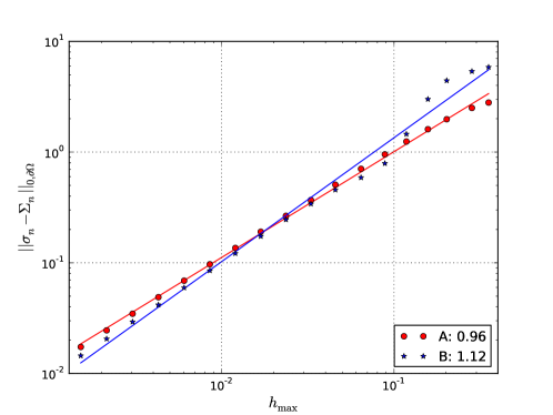
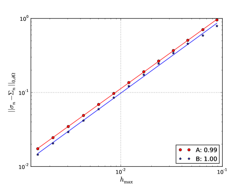
Fig. 7.1: $L^{2}(\partial\Omega)$ convergence study for various flux computations. (A) Nitsche flux for $\mathrm{CG}(1)$ elements. (B) Lagrange multiplier computed with the stabilized method by Barbosa and Hughes based on a $\mathrm{CG}(1)\times\mathrm{DG}(0)$ discretization. The legend gives the fitted slope for each approximation error. (Left) Approximation error for the entire mesh sequence revealing different behavior in the pre-asymptotic regime. (Right) Asymptotic regime. Starting from $h\approx 0.1$ both methods give optimal first order convergence.

References

• Babuška [1973] I. Babuška. The finite element method with Lagrangian multipliers. Num. Math., 20(3):179–192, June 1973.
• Barbosa and Hughes [1991] H.J.C. Barbosa and T.J.R. Hughes. The finite element method with Lagrange multipliers on the boundary: circumventing the Babuška-Brezzi condition. Computer Methods in Applied Mechanics and Engineering, 85(1):109–128, 1991.
• Barbosa and Hughes [1992] H.J.C. Barbosa and T.J.R. Hughes. Boundary Lagrange multipliers in finite element methods: error analysis in natural norms. Numer. Math., 62(1):1–15, 1992.
• Bramble [1981] J.H. Bramble. The Lagrange multiplier method for Dirichlet’s problem. Math. Comput., 37(155):1–11, 1981.
• Brezzi [1974] F. Brezzi. On the Existence, Uniqueness and Approximation of Saddle-Point Problems Arising from Lagrangian Multipliers. RAIRO Anal. Numér., R–2:129–151, 1974.
• Burman [2013] Erik Burman. Projection stabilization of Lagrange multipliers for the imposition of constraints on interfaces and boundaries. Numerical Methods for Partial Differential Equations, pages n/a–n/a, 2013.
• Carey et al. [1985] G.F. Carey, S.S. Chow, and M.K. Seager. Approximate boundary-flux calculations. Computer Methods in Applied Mechanics and Engineering, 50(2):107–120, 1985.
• Chabrowski [1982] J. Chabrowski. Note on the Dirichlet problem with L2-boundary data. Manuscripta Math., 108(40):91–108, 1982.
• Chabrowski [1991] J. Chabrowski. The Dirichlet Problem with L2-Boundary Data for Elliptic Linear Equations, volume 1482 of Lecture Notes in Mathematics. Springer, 1991.
• Estep et al. [2010] D. Estep, S. Tavener, and T. Wildey. A posteriori error estimation and adaptive mesh refinement for a multiscale operator decomposition approach to fluid–solid heat transfer. Journal of Computational Physics, 229(11):4143–4158, 2010.
• Gilbard and Trudinger [2001] D. Gilbard and N.S. Trudinger. Elliptic partial differential equations of second order, volume 224 of Classics in Mathematics. Springer, 2001.
• Giles et al. [1997] M. Giles, M.G. Larson, M. Levenstam, and E. Süli. Adaptive error control for finite element approximations of the lift and drag coefficients in viscous flow. Technical report, The Mathematical Institute, University of Oxford, 1997.
• Hansbo and Hansbo [2002] A. Hansbo and P. Hansbo. An unfitted finite element method, based on Nitsche’s method, for elliptic interface problems. Comput. Methods Appl. Mech. Engrg., 191(47-48):5537–5552, 2002.
• Hansbo [2005] P. Hansbo. Nitsche’s method for interface problems in computational mechanics. GAMM-Mitt, 28(2):183–206, 2005.
• Melenk and Wohlmuth [2012] J.M. Melenk and B. Wohlmuth. Quasi-optimal approximation of surface based Lagrange multipliers in finite element methods. SIAM J. Numer. Anal., 50(4):2064–2087, 2012.
• Nitsche [1971] J. Nitsche. Über ein Variationsprinzip zur Lösung von Dirichlet-Problemen bei Verwendung von Teilräumen, die keinen Randbedingungen unterworfen sind. Abhandlungen aus dem Mathematischen Seminar der Universität Hamburg, 36(1):9–15, July 1971.
• Pehlivanov et al. [1992] A.I. Pehlivanov, R.D. Lazarov, G.F. Carey, and S.S. Chow. Superconvergence analysis of approximate boundary-flux calculations. Numerische Mathematik, 63(1):483–501, 1992.
• Pitkäranta [1979] J. Pitkäranta. Boundary subspaces for the finite element method with Lagrange multipliers. Numer. Math., 289(33):273–289, 1979.
• Pitkäranta [1980] J. Pitkäranta. Local stability conditions for the Babuška method of Lagrange multipliers. Math. Comp., 35(152):1113–1129, 1980.
• Rannacher and Scott [1982] R. Rannacher and R. Scott. Some optimal error estimates for piecewise linear finite element approximations. Math. Comp., 38(158):437–445, 1982.
• Scott and Zhang [1990] R. Scott and S. Zhang. Finite element interpolation of nonsmooth functions satisfying boundary conditions. Math. Comp., 54(190):483–493, 1990.
• Stenberg [1995] R. Stenberg. On some techniques for approximating boundary conditions in the finite element method. J. Comput. Appl. Math., 63(1):139–148, 1995.