Perturbation Analysis and Randomized Algorithms for Large-Scale Total Least Squares Problems

Pengpeng Xiea  Yimin Weia,b  Hua Xiangc

a School of Mathematical Sciences, Fudan University, Shanghai, 200433, P.R. China
band Key Laboratory of Mathematics for Nonlinear Sciences
c School of Mathematics and Statistics, Wuhan University, Wuhan, 430072, P.R. China
E-mail: 09110180005@fudan.edu.cn. P. Xie is supported by the National Natural Science Foundation of China under grant 11271084.E-mall: ymwei@fudan.edu.cn. Y. Wei is supported by the National Natural Science Foundation of China under grant 11271084.Corresponding author (H. Xiang). E-mail: hxiang@whu.edu.cn. H. Xiang is supported by the National Natural Science Foundation of China under grants 10901125 and 91130022. Partial work was completed when he visited Fudan University and The Chinese University of Hong Kong in 2014.
Abstract

In this paper, we present perturbation analysis and randomized algorithms for the total least squares (Tls) problems. We derive the perturbation bound and check its sharpness by numerical experiments. Motivated by the recently popular probabilistic algorithms for low-rank approximations, we develop randomized algorithms for the Tls and the truncated total least squares (Ttls) solutions of large-scale discrete ill-posed problems, which can greatly reduce the computational time and still keep good accuracy.

Keywords: Condition number; Singular value decomposition; Total least squares; Truncated total least squares; Randomized algorithms.

AMS Classification: 15A09, 65F35

1 Introduction

Given an overdetermined set of m𝑚m linear equations Axb𝐴𝑥𝑏Ax\approx b in n𝑛n unknowns x,𝑥x, the total least squares (Tls) problem can be formulated as [38]

min[Ef]Fsubscriptnormdelimited-[]𝐸𝑓𝐹\displaystyle\min\left\|~{}[E\ f]~{}\right\|_{F} subject to b+f(A+E),𝑏𝑓𝐴𝐸\displaystyle\quad b+f\in\mathscr{R}(A+E), (1.1)

where F\|\cdot\|_{F} denotes the Frobenius matrix norm and ()\mathscr{R}(\cdot) represents the range space. When the sampling or modeling or measurement errors also affect the coefficient matrix A,𝐴A, the Tls method is more realistic, while the underlying assumption in the least squares (Ls) problem is that errors only occur in the right-hand side vector b𝑏b.

The term “total least squares” was coined in [11]. It has been also known as errors-in-variables model, orthogonal regression, or measurement errors in the statistical literature, and blind deconvolution in image deblurring. In the monograph [38] the authors show the readers how to use Tls for solving a variety of problems, especially those arising in signal processing, medical imaging, and geophysics, etc. The applications and theory associated with the Tls are still being studied, for example [16, 23]. In recent years, perturbation analysis for the Tls problem has been studied extensively in the numerical linear algebra (see e.g. [2, 6, 7, 13, 17, 24, 28, 31, 33, 40, 39, 43, 44]).

It is well known that the condition number indicates the sensitivity of the problem itself, and that an approximate bound for the forward error can be given by the multiplication of the condition number and the backward error. For the perturbation in the solution of the scaled total least squares problem, Zhou et al. [44] presented a first order estimation. But as pointed out by the authors, it is not easy to compute since the condition number formula is a Kronecker product-based one. Baboulin and Gratton [2] derived a computable expression for the condition number. At almost the same time, Li and Jia [24] made a first order perturbation analysis. Recently, Jia and Li [18] proposed a formula which only used the singular values and the right singular vectors of [A,b]𝐴𝑏[A,~{}b], and presented the lower and upper bounds for the condition number. In this paper, we will present a relative perturbation bound without considering the condition number only. We first give a perturbation bound in this paper. And its significant improvements will be demonstrated by numerical examples. We also show that these three condition numbers in [2, 24, 44] mentioned above are mathematically equivalent.

For the numerical solution of the Tls problem, a simple and elegant solver based on the Svd of the augmented matrix [A,b]𝐴𝑏[A,~{}b] can be used. When A𝐴A is large, a complete Svd will be very costly. One improvement is to compute a partial Svd based on Lanczos bi-diagonalization [9]. But the partial Svd is still prohibitive for large-scale sparse or structured matrices, since the initial reduction of [A,b]𝐴𝑏[A,~{}b] to bi-diagonal form will destroy the sparsity or structure of the matrix. For the Tls problem with very ill-conditioned coefficient matrix whose singular values decay gradually, the task is even more challenging. Without regularization, the ordinary least squares or total least squares solvers yield physically meaningless solutions. For such discrete ill-posed problems, there already exist several regularization strategies of the Tls solution. For example, the solution can be stabilized by truncating small singular values of [A,b]𝐴𝑏[A,~{}b] via an iterative algorithm based on Lanczos bi-diagonalization [9]. Tikhonov regularization strategy is used in [4, 10, 22, 23, 29], where a Cholesky decomposition is computed in each step in [4], and the linear systems are projected onto Krylov subpace of much smaller dimensions to reduce the problem size in [22]. Regularization by an additional quadratic constraint is another choice [5, 21, 35, 36], which is the regularized Tls based on quadratic eigenvalue problems (Qep): adding a quadratic constraint to the Tls, and then iteratively solving the Qep. For the large-scale discrete ill-conditioned problem, a complete Svd is prohibitive, and the choice of regularization parameter is also time consuming. The classical Svd of a matrix can be well approximated by the randomized Svd [14], and the regularization parameter can also be located by randomized algorithms [42]. Such randomized algorithms can greatly reduce the computational time, and still keep good accuracy with very high probability. Motivated by these randomized matrix algorithms, we present randomized algorithms for the solution of total least squares (Tls) problems including the well-conditioned cases and the ill-conditioned cases. For the practical cases where the numerical rank is not known, randomized algorithms can usually be implemented in an adaptive approach with the sample number increasing until the desired tolerance is satisfied. Here the tolerance parameter is adopted to describe how well the basis matrix generated by the randomization captures the action of the target matrix. Based on this, we develop the randomized algorithm for the fixed precision cases.

Throughout this paper, m×nsuperscript𝑚𝑛\mathbb{R}^{m\times n} denotes the set of m×n𝑚𝑛m\times n matrices with real entries and Insubscript𝐼𝑛I_{n} stands for the identity matrix with order n.𝑛n. As usual, 𝟎0{\bf 0} denotes the zero matrix with the corresponding size easily known from the context. For a matrix Am×n,𝐴superscript𝑚𝑛A\in\mathbb{R}^{m\times n}, ATsuperscript𝐴TA^{\mathrm{T}} is the transpose of A𝐴A; A2subscriptnorm𝐴2\|A\|_{2}, AFsubscriptnorm𝐴𝐹\|A\|_{F} and Asubscriptnorm𝐴\|A\|_{\infty} denote the spectral norm, the Frobenius norm and the infinity norm of A𝐴A, respectively. And Asuperscript𝐴A^{\dagger} represents the Moore-Penrose inverse of A𝐴A [12] and λmax(A)subscript𝜆𝐴\lambda_{\max}\left(A\right) denotes the largest eigenvalue of A𝐴A. For any matrix A=[a1,a2,,an]=(aij)m×n𝐴subscript𝑎1subscript𝑎2subscript𝑎𝑛subscript𝑎𝑖𝑗superscript𝑚𝑛A=\left[a_{1},a_{2},\ldots,a_{n}\right]=\left(a_{ij}\right)\in\mathbb{R}^{m\times n} and B=(bij)p×q,𝐵subscript𝑏𝑖𝑗superscript𝑝𝑞B=\left(b_{ij}\right)\in\mathbb{R}^{p\times q}, the Kronecker product ABtensor-product𝐴𝐵A\otimes B is defined as AB=(aijB)mp×nq.tensor-product𝐴𝐵subscript𝑎𝑖𝑗𝐵superscript𝑚𝑝𝑛𝑞A\otimes B=\left(a_{ij}B\right)\in\mathbb{R}^{mp\times nq}. We define vec(A)=[a1T,a2T,,anT]Tmn.vec𝐴superscriptsuperscriptsubscript𝑎1Tsuperscriptsubscript𝑎2Tsuperscriptsubscript𝑎𝑛TTsuperscript𝑚𝑛\mathrm{vec}(A)=\left[a_{1}^{\mathrm{T}},a_{2}^{\mathrm{T}},\ldots,a_{n}^{\mathrm{T}}\right]^{\mathrm{T}}\in\mathbb{R}^{mn}. For a vector a,𝑎a, diag(a)diag𝑎\textrm{diag}(a) is a diagonal matrix whose diagonals are given as components of a.𝑎a. The remaining sections of this paper are organized as follows. Section 2 introduces some basic results. In section 3, we present our main perturbation results and show the mathematical equivalence of three kinds of condition numbers. We turn to the randomized algorithms in section 4 and the detailed error analysis for Algorithm Rttls is given. The numerical results are performed in section 5 and section 6 concludes this paper.

2 Preliminaries

Let Am×n𝐴superscript𝑚𝑛A\in\mathbb{R}^{m\times n} and bm𝑏superscript𝑚b\in\mathbb{R}^{m} with mn.𝑚𝑛m\geq n. Let [A,b]𝐴𝑏[A,~{}b] and A𝐴A have singular value decompositions, respectively

UT[A,b]V=diag(σ1,σ2,,σt)=Σ,superscript𝑈T𝐴𝑏𝑉diagsubscript𝜎1subscript𝜎2subscript𝜎𝑡ΣU^{\mathrm{T}}[A,~{}b]V=\textrm{diag}\left(\sigma_{1},\sigma_{2},\ldots,\sigma_{t}\right)=\Sigma,
U~TAV~=diag(σ~1,σ~2,,σ~n),superscript~𝑈T𝐴~𝑉diagsubscript~𝜎1subscript~𝜎2subscript~𝜎𝑛\widetilde{U}^{\mathrm{T}}A\widetilde{V}=\textrm{diag}\left(\widetilde{\sigma}_{1},\widetilde{\sigma}_{2},\ldots,\widetilde{\sigma}_{n}\right),

where t=min{m,n+1}𝑡𝑚𝑛1t=\min\{m,n+1\} and for the case m>n,𝑚𝑛m>n, orthonormal matrices U𝑈U and V,𝑉V, diagonal matrix ΣΣ\Sigma are partitioned as follows:

U=[U1,un+1]m×(n+1),𝑈subscriptsubscript𝑈1subscript𝑢𝑛1𝑚𝑛1\displaystyle U=\left[U_{1},u_{n+1}\right]_{m\times(n+1)}, V=[V11v12v21v22](n+1)×(n+1),𝑉subscriptdelimited-[]subscript𝑉11subscript𝑣12subscript𝑣21subscript𝑣22𝑛1𝑛1\displaystyle V=\left[\begin{array}[]{cc}V_{11}&v_{12}\\ v_{21}&v_{22}\end{array}\right]_{(n+1)\times(n+1)}, Σ=[Σ1𝟎𝟎σn+1].Σdelimited-[]subscriptΣ100subscript𝜎𝑛1\displaystyle\Sigma=\left[\begin{array}[]{cc}\Sigma_{1}&{\bf 0}\\ {\bf 0}&\sigma_{n+1}\end{array}\right].

For the usual well-conditioned cases in this paper, we assume the genericity condition:

σ~n>σn+1,subscript~𝜎𝑛subscript𝜎𝑛1\widetilde{\sigma}_{n}>\sigma_{n+1}, (2.2)

to ensure the existence and uniqueness of the Tls solution x𝑥x (see [11]). The singular value σn+1subscript𝜎𝑛1\sigma_{n+1} can be treated as 0 for the case m=n𝑚𝑛m=n since σn+1subscript𝜎𝑛1\sigma_{n+1} does not exist at all. From best rank-1 approximation [12] of matrix [A,b]𝐴𝑏[A,~{}b], we know that

[E,f]𝐸𝑓\displaystyle[E,~{}f] =\displaystyle= U[𝟎𝟎𝟎σn+1]VT𝑈delimited-[]000subscript𝜎𝑛1superscript𝑉T\displaystyle-U\left[\begin{array}[]{cc}{\bf 0}&{\bf 0}\\ {\bf 0}&\sigma_{n+1}\end{array}\right]V^{\mathrm{T}}
=\displaystyle= σn+1un+1[v12T,v22]subscript𝜎𝑛1subscript𝑢𝑛1superscriptsubscript𝑣12Tsubscript𝑣22\displaystyle-\sigma_{n+1}u_{n+1}\left[v_{12}^{\mathrm{T}},\quad v_{22}\right]
=\displaystyle= σn+1un+1vn+1T,subscript𝜎𝑛1subscript𝑢𝑛1superscriptsubscript𝑣𝑛1T\displaystyle-\sigma_{n+1}u_{n+1}v_{n+1}^{\mathrm{T}},

where vn+1=[v12T,v22]Tsubscript𝑣𝑛1superscriptsuperscriptsubscript𝑣12Tsubscript𝑣22Tv_{n+1}=\left[v_{12}^{\mathrm{T}},\quad v_{22}\right]^{\mathrm{T}}. Therefore, x=v12/v22.𝑥subscript𝑣12subscript𝑣22x=-v_{12}/v_{22}. It follows from [38, Theorem 2.7] that the solution x𝑥x can also be expressed as a function of [A,b]𝐴𝑏[A,~{}b], i.e.,

x𝑥\displaystyle x =\displaystyle= (ATAσn+12I)1ATb,superscriptsuperscript𝐴T𝐴superscriptsubscript𝜎𝑛12𝐼1superscript𝐴T𝑏\displaystyle\left(A^{\mathrm{T}}A-\sigma_{n+1}^{2}I\right)^{-1}A^{\mathrm{T}}b, (2.4)

and it holds that

[xT,1]Tsuperscriptsuperscript𝑥T1T\displaystyle\left[x^{\mathrm{T}},~{}-1\right]^{\mathrm{T}} =\displaystyle= 1v22vn+1.1subscript𝑣22subscript𝑣𝑛1\displaystyle-\frac{1}{v_{22}}v_{n+1}. (2.5)

In the case m=n𝑚𝑛m=n under the genericity condition, the original system is just a nonsingular one and the Tls solution is equal to the least squares solution. Now consider the Tls problem (1.1) and assume σ~q>σq+1==σn+1subscript~𝜎𝑞subscript𝜎𝑞1subscript𝜎𝑛1\widetilde{\sigma}_{q}>\sigma_{q+1}=\cdots=\sigma_{n+1} with qn.𝑞𝑛q\leq n. Let the above Svd still hold but partition V𝑉V differently as follows:

V𝑉\displaystyle V =\displaystyle= [V11v21V12v22]n1qn+1q.\displaystyle\begin{array}[]{@{}r@{}c@{}c@{}c@{}l@{}}\left[\begin{array}[]{c}\\ \\ \end{array}\right.&\begin{array}[]{c}V_{11}\\ v_{21}\end{array}&\begin{array}[]{c}\\ \end{array}&\begin{array}[]{c}V_{12}\\ v_{22}\end{array}&\left]\begin{array}[]{c}n\\ 1\end{array}\right.\\ &q&&n\!+\!1\!-\!q\end{array}. (2.17)

The condition σ~q>σq+1==σn+1subscript~𝜎𝑞subscript𝜎𝑞1subscript𝜎𝑛1\widetilde{\sigma}_{q}>\sigma_{q+1}=\cdots=\sigma_{n+1} is equivalent to that σq>σq+1==σn+1subscript𝜎𝑞subscript𝜎𝑞1subscript𝜎𝑛1\sigma_{q}>\sigma_{q+1}=\cdots=\sigma_{n+1} and v22subscript𝑣22v_{22} is of full row rank, i.e., v22subscript𝑣22v_{22} is not a zero vector. According to [38, Theorem 3.10], the minimum norm Tls solution x¯¯𝑥\bar{x} is given by

x¯¯𝑥\displaystyle\bar{x} =\displaystyle= V12v22=(V11T)v21T.subscript𝑉12superscriptsubscript𝑣22superscriptsuperscriptsubscript𝑉11Tsuperscriptsubscript𝑣21T\displaystyle-V_{12}v_{22}^{\dagger}=\left(V_{11}^{\mathrm{T}}\right)^{\dagger}v_{21}^{\mathrm{T}}.

This is called the truncated total least squares (Ttls). The case m<n+1𝑚𝑛1m<n+1 requires that σn+1=0subscript𝜎𝑛10\sigma_{n+1}=0 and hence [E,f]F=0subscriptnorm𝐸𝑓𝐹0\|[E,~{}f]\|_{F}=0 [38]. The idea of Ttls is to treat the small singular values of the augmented matrix [A,b]𝐴𝑏[A,~{}b] as zeros and convert a numerically rank-deficient problem to an exactly rank-deficient one. For the discrete ill-posed problems where the singular values of the coefficient matrices decay gradually, Ttls can be applied, where the parameter q𝑞q then plays the role of the regularization parameter. In practical applications, the smallest singular values of [A,b]𝐴𝑏[A,~{}b] rarely coincide [39]. But if one considers the Tls problem as an approximation to the corresponding unobservable exact relation A0x=b0,subscript𝐴0𝑥subscript𝑏0A_{0}x=b_{0}, then rank([A0,b0])=rank(A0)=qn.ranksubscript𝐴0subscript𝑏0ranksubscript𝐴0𝑞𝑛\mbox{rank}\left([A_{0},~{}b_{0}]\right)=\mbox{rank}\left(A_{0}\right)=q\leq n. So σq+1,,σn+1subscript𝜎𝑞1subscript𝜎𝑛1\sigma_{q+1},\ldots,\sigma_{n+1} are just the perturbations of zero. In this case it is realistic to define an error bound ϵitalic-ϵ\epsilon such that all singular values σi,subscript𝜎𝑖\sigma_{i}, satisfying |σiσn+1|<ϵ,subscript𝜎𝑖subscript𝜎𝑛1italic-ϵ\left|\sigma_{i}-\sigma_{n+1}\right|<\epsilon, are considered to coincide with σn+1.subscript𝜎𝑛1\sigma_{n+1}. Therefore, we can use the formula x¯=V12v22.¯𝑥subscript𝑉12superscriptsubscript𝑣22\bar{x}=-V_{12}v_{22}^{\dagger}.

3 Perturbation results

First, we give a lemma which will be very useful in our analysis.

Lemma 3.1

Consider the total least squares problem (1.1) and assume that the genericity condition (2.2) holds. If [A,b]𝐴𝑏~{}[A,~{}b] is perturbed to [A+δA,b+δb]𝐴𝛿𝐴𝑏𝛿𝑏[A+\delta A,~{}b+\delta b], then we have

σn+1un+1T[δA,δb]vn+1subscript𝜎𝑛1superscriptsubscript𝑢𝑛1T𝛿𝐴𝛿𝑏subscript𝑣𝑛1\displaystyle\sigma_{n+1}u_{n+1}^{\mathrm{T}}[\delta A,~{}\delta b]v_{n+1} =\displaystyle= rT[δb(δA)x]1+xTx,superscript𝑟Tdelimited-[]𝛿𝑏𝛿𝐴𝑥1superscript𝑥T𝑥\displaystyle\frac{r^{\mathrm{T}}[\delta b-(\delta A)x]}{1+x^{\mathrm{T}}x},

where r=bAx.𝑟𝑏𝐴𝑥r=b-Ax.

Proof.  From (2.5) and the singular value decomposition of [A,b]𝐴𝑏[A,~{}b], we know that

r=bAx=[A,b][x1]=1v22[A,b]vn+1=1v22σn+1un+1.𝑟𝑏𝐴𝑥𝐴𝑏delimited-[]𝑥11subscript𝑣22𝐴𝑏subscript𝑣𝑛11subscript𝑣22subscript𝜎𝑛1subscript𝑢𝑛1r=b-Ax=-[A,~{}b]\left[\begin{array}[]{c}x\\ -1\end{array}\right]=\frac{1}{v_{22}}[A,~{}b]v_{n+1}=\frac{1}{v_{22}}\sigma_{n+1}u_{n+1}.

Therefore we have

rT[δb(δA)x]1+xTxsuperscript𝑟Tdelimited-[]𝛿𝑏𝛿𝐴𝑥1superscript𝑥T𝑥\displaystyle\frac{r^{\mathrm{T}}[\delta b-(\delta A)x]}{1+x^{\mathrm{T}}x} =\displaystyle= σn+1v22un+1T[δb(δA)x]1+xTxsubscript𝜎𝑛1subscript𝑣22superscriptsubscript𝑢𝑛1Tdelimited-[]𝛿𝑏𝛿𝐴𝑥1superscript𝑥T𝑥\displaystyle\frac{\sigma_{n+1}}{v_{22}}\frac{u_{n+1}^{\mathrm{T}}[\delta b-(\delta A)x]}{1+x^{\mathrm{T}}x}
=\displaystyle= σn+1v22un+1T[δA,δb][x1]subscript𝜎𝑛1subscript𝑣22superscriptsubscript𝑢𝑛1T𝛿𝐴𝛿𝑏delimited-[]𝑥1\displaystyle-\sigma_{n+1}v_{22}u_{n+1}^{\mathrm{T}}[\delta A,~{}\delta b]\left[\begin{array}[]{c}x\\ -1\end{array}\right]
=\displaystyle= σn+1un+1T[δA,δb]vn+1,subscript𝜎𝑛1superscriptsubscript𝑢𝑛1T𝛿𝐴𝛿𝑏subscript𝑣𝑛1\displaystyle\sigma_{n+1}u_{n+1}^{\mathrm{T}}[\delta A,~{}\delta b]v_{n+1},

where we use v222=11+xTxsuperscriptsubscript𝑣22211superscript𝑥T𝑥v_{22}^{2}=\frac{1}{1+x^{\mathrm{T}}x}, which is a direct result of (2.5).        \Box

The following lemma [37] is also needed for deriving our perturbation result.

Lemma 3.2

Let σminsubscript𝜎\sigma_{\min} be the smallest nonzero and simple singular value of a matrix X𝑋X with uminsubscript𝑢u_{\min} and vminsubscript𝑣v_{\min} being its corresponding left and right singular vectors, respectively. If δXFsubscriptnorm𝛿𝑋𝐹\left\|\delta X\right\|_{F} is sufficiently small, then the smallest nonzero singular value σ^minsubscript^𝜎\widehat{\sigma}_{\min} of the perturbed matrix X^=X+δX^𝑋𝑋𝛿𝑋\widehat{X}=X+\delta X is simple and

σ^minsubscript^𝜎\displaystyle\widehat{\sigma}_{\min} =\displaystyle= σmin+uminT(δX)vmin+𝒪(δXF2).subscript𝜎superscriptsubscript𝑢T𝛿𝑋subscript𝑣𝒪superscriptsubscriptnorm𝛿𝑋𝐹2\displaystyle\sigma_{\min}+u_{\min}^{\mathrm{T}}(\delta X)v_{\min}+\mathcal{O}\left(\left\|\delta X\right\|_{F}^{2}\right).

In the following, we present our perturbation bound under the genericity condition (2.2).

Theorem 3.1

Consider the total least squares problem (1.1) and assume that the genericity condition (2.2) holds. If [δA,δb]Fsubscriptnorm𝛿𝐴𝛿𝑏𝐹\left\|[\delta A,~{}\delta b]\right\|_{F} is sufficiently small, then we have that

δx2x2subscriptnorm𝛿𝑥2subscriptnorm𝑥2\displaystyle\frac{\|\delta x\|_{2}}{\|x\|_{2}} less-than-or-similar-to\displaystyle\lesssim (b2x2(ATAσn+12I)1AT2)δb2b2subscriptnorm𝑏2subscriptnorm𝑥2subscriptnormsuperscriptsuperscript𝐴T𝐴superscriptsubscript𝜎𝑛12𝐼1superscript𝐴T2subscriptnorm𝛿𝑏2subscriptnorm𝑏2\displaystyle\left(\frac{\|b\|_{2}}{\|x\|_{2}}\left\|\left(A^{\mathrm{T}}A-\sigma_{n+1}^{2}I\right)^{-1}A^{\mathrm{T}}\right\|_{2}\right)\frac{\|\delta b\|_{2}}{\|b\|_{2}} (3.2)
+\displaystyle+ [A2r2x2(ATAσn+12I)12+A2(ATAσn+12I)1AT2]δA2A2,delimited-[]subscriptnorm𝐴2subscriptnorm𝑟2subscriptnorm𝑥2subscriptnormsuperscriptsuperscript𝐴T𝐴superscriptsubscript𝜎𝑛12𝐼12subscriptnorm𝐴2subscriptnormsuperscriptsuperscript𝐴T𝐴superscriptsubscript𝜎𝑛12𝐼1superscript𝐴T2subscriptnorm𝛿𝐴2subscriptnorm𝐴2\displaystyle\left[\frac{\|A\|_{2}\|r\|_{2}}{\|x\|_{2}}\left\|\left(A^{\mathrm{T}}A-\sigma_{n+1}^{2}I\right)^{-1}\right\|_{2}+\|A\|_{2}\left\|\left(A^{\mathrm{T}}A-\sigma_{n+1}^{2}I\right)^{-1}A^{\mathrm{T}}\right\|_{2}\right]\frac{\|\delta A\|_{2}}{\|A\|_{2}},

where r=bAx.𝑟𝑏𝐴𝑥r=b-Ax.

Proof.  From (ATAσn+12I)x=ATb,superscript𝐴T𝐴superscriptsubscript𝜎𝑛12𝐼𝑥superscript𝐴T𝑏\left(A^{\mathrm{T}}A-\sigma_{n+1}^{2}I\right)x=A^{\mathrm{T}}b, perturbing [A,b]𝐴𝑏[A,~{}b] yields

[(A+δA)T(A+δA)σ^n+12In](x+δx)=(A+δA)T(b+δb),delimited-[]superscript𝐴𝛿𝐴T𝐴𝛿𝐴superscriptsubscript^𝜎𝑛12subscript𝐼𝑛𝑥𝛿𝑥superscript𝐴𝛿𝐴T𝑏𝛿𝑏\displaystyle\left[(A+\delta A)^{\mathrm{T}}(A+\delta A)-\widehat{\sigma}_{n+1}^{2}I_{n}\right](x+\delta x)=(A+\delta A)^{\mathrm{T}}(b+\delta b), (3.3)

where σ^n+1subscript^𝜎𝑛1\widehat{\sigma}_{n+1} is the smallest singular value of [A+δA,b+δb].𝐴𝛿𝐴𝑏𝛿𝑏[A+\delta A,~{}b+\delta b]. Subtracting two equations (2.4) and (3.3), we have

(ATAσn+12In)δxsuperscript𝐴T𝐴superscriptsubscript𝜎𝑛12subscript𝐼𝑛𝛿𝑥\displaystyle\left(A^{\mathrm{T}}A-\sigma_{n+1}^{2}I_{n}\right)\delta x =\displaystyle= (δA)Tr+AT[δb(δA)x]+(σ^n+12σn+12)(x+δx)superscript𝛿𝐴T𝑟superscript𝐴Tdelimited-[]𝛿𝑏𝛿𝐴𝑥superscriptsubscript^𝜎𝑛12superscriptsubscript𝜎𝑛12𝑥𝛿𝑥\displaystyle(\delta A)^{\mathrm{T}}r+A^{\mathrm{T}}\left[\delta b-(\delta A)x\right]+\left(\widehat{\sigma}_{n+1}^{2}-\sigma_{n+1}^{2}\right)(x+\delta x) (3.4)
+\displaystyle+ 𝒪([δA,δb]F2).𝒪superscriptsubscriptnorm𝛿𝐴𝛿𝑏𝐹2\displaystyle{\mathcal{O}}\left(\left\|[\delta A,~{}\delta b]\right\|_{F}^{2}\right).

Furthermore, combining Lemma 3.1 and Lemma 3.2, we have

σ^n+12σn+12superscriptsubscript^𝜎𝑛12superscriptsubscript𝜎𝑛12\displaystyle\widehat{\sigma}_{n+1}^{2}-\sigma_{n+1}^{2} =\displaystyle= (σ^n+1σn+1)(σ^n+1+σn+1)subscript^𝜎𝑛1subscript𝜎𝑛1subscript^𝜎𝑛1subscript𝜎𝑛1\displaystyle\left(\widehat{\sigma}_{n+1}-\sigma_{n+1}\right)\left(\widehat{\sigma}_{n+1}+\sigma_{n+1}\right) (3.5)
=\displaystyle= {un+1T[δA,δb]vn+1+𝒪([δA,δb]F2)}{2σn+1+un+1T[δA,δb]vn+1+𝒪([δA,δb]F2)}superscriptsubscript𝑢𝑛1T𝛿𝐴𝛿𝑏subscript𝑣𝑛1𝒪superscriptsubscriptnorm𝛿𝐴𝛿𝑏𝐹22subscript𝜎𝑛1superscriptsubscript𝑢𝑛1T𝛿𝐴𝛿𝑏subscript𝑣𝑛1𝒪superscriptsubscriptnorm𝛿𝐴𝛿𝑏𝐹2\displaystyle\left\{u_{n+1}^{\mathrm{T}}[\delta A,~{}\delta b]v_{n+1}+{\mathcal{O}}\left(\left\|[\delta A,~{}\delta b]\right\|_{F}^{2}\right)\right\}\left\{2\sigma_{n+1}+u_{n+1}^{\mathrm{T}}[\delta A,~{}\delta b]v_{n+1}+{\mathcal{O}}\left(\left\|[\delta A,~{}\delta b]\right\|_{F}^{2}\right)\right\}
=\displaystyle= 2rT[δb(δA)x]1+xTx+𝒪([δA,δb]F2),2superscript𝑟Tdelimited-[]𝛿𝑏𝛿𝐴𝑥1superscript𝑥T𝑥𝒪superscriptsubscriptnorm𝛿𝐴𝛿𝑏𝐹2\displaystyle 2\frac{r^{\mathrm{T}}[\delta b-(\delta A)x]}{1+x^{\mathrm{T}}x}+{\mathcal{O}}\left(\left\|[\delta A,~{}\delta b]\right\|_{F}^{2}\right),

where for the last approximation we use Lemma 3.1. From (3.4) and (3.5), ignoring higher order terms, we know that

δx𝛿𝑥\displaystyle\delta x \displaystyle\approx (ATAσn+12In)1{[AT(δb(δA)x)+(δA)Tr]+2rT[δb(δA)x]1+xTx(x+δx)}superscriptsuperscript𝐴T𝐴superscriptsubscript𝜎𝑛12subscript𝐼𝑛1delimited-[]superscript𝐴T𝛿𝑏𝛿𝐴𝑥superscript𝛿𝐴T𝑟2superscript𝑟Tdelimited-[]𝛿𝑏𝛿𝐴𝑥1superscript𝑥T𝑥𝑥𝛿𝑥\displaystyle\left(A^{\mathrm{T}}A-\sigma_{n+1}^{2}I_{n}\right)^{-1}\left\{\left[A^{\mathrm{T}}\left(\delta b-(\delta A)x\right)+(\delta A)^{\mathrm{T}}r\right]+2\dfrac{r^{\mathrm{T}}[\delta b-(\delta A)x]}{1+x^{\mathrm{T}}x}(x+\delta x)\right\}
\displaystyle\approx (ATAσn+12In)1[AT(δb)AT(δA)x+(δA)Tr]+2(ATAσn+12In)1rT[δb(δA)x]1+xTxxsuperscriptsuperscript𝐴T𝐴superscriptsubscript𝜎𝑛12subscript𝐼𝑛1delimited-[]superscript𝐴T𝛿𝑏superscript𝐴T𝛿𝐴𝑥superscript𝛿𝐴T𝑟2superscriptsuperscript𝐴T𝐴superscriptsubscript𝜎𝑛12subscript𝐼𝑛1superscript𝑟Tdelimited-[]𝛿𝑏𝛿𝐴𝑥1superscript𝑥T𝑥𝑥\displaystyle\left(A^{\mathrm{T}}A-\sigma_{n+1}^{2}I_{n}\right)^{-1}\left[A^{\mathrm{T}}(\delta b)-A^{\mathrm{T}}(\delta A)x+(\delta A)^{\mathrm{T}}r\right]+2\left(A^{\mathrm{T}}A-\sigma_{n+1}^{2}I_{n}\right)^{-1}\dfrac{r^{\mathrm{T}}\left[\delta b-(\delta A)x\right]}{1+x^{\mathrm{T}}x}x
=\displaystyle= (ATAσn+12In)1[AT+2xrT1+xTx]δb+(ATAσn+12In)1[(δA)Tr(AT+2xrT1+xTx)(δA)x].superscriptsuperscript𝐴T𝐴superscriptsubscript𝜎𝑛12subscript𝐼𝑛1delimited-[]superscript𝐴T2𝑥superscript𝑟T1superscript𝑥T𝑥𝛿𝑏superscriptsuperscript𝐴T𝐴superscriptsubscript𝜎𝑛12subscript𝐼𝑛1delimited-[]superscript𝛿𝐴T𝑟superscript𝐴T2𝑥superscript𝑟T1superscript𝑥T𝑥𝛿𝐴𝑥\displaystyle\left(A^{\mathrm{T}}A-\sigma_{n+1}^{2}I_{n}\right)^{-1}\left[A^{\mathrm{T}}+2\dfrac{xr^{\mathrm{T}}}{1+x^{\mathrm{T}}x}\right]\delta b+\left(A^{\mathrm{T}}A-\sigma_{n+1}^{2}I_{n}\right)^{-1}\left[(\delta A)^{\mathrm{T}}r-\left(A^{\mathrm{T}}+2\dfrac{xr^{\mathrm{T}}}{1+x^{\mathrm{T}}x}\right)(\delta A)x\right].

Hence,

δx2subscriptnorm𝛿𝑥2\displaystyle\|\delta x\|_{2} less-than-or-similar-to\displaystyle\lesssim (ATAσn+12In)1[AT+2xrT1+xTx]2δb2subscriptnormsuperscriptsuperscript𝐴T𝐴superscriptsubscript𝜎𝑛12subscript𝐼𝑛1delimited-[]superscript𝐴T2𝑥superscript𝑟T1superscript𝑥T𝑥2subscriptnorm𝛿𝑏2\displaystyle\left\|\left(A^{\mathrm{T}}A-\sigma_{n+1}^{2}I_{n}\right)^{-1}\left[A^{\mathrm{T}}+2\dfrac{xr^{\mathrm{T}}}{1+x^{\mathrm{T}}x}\right]\right\|_{2}\|\delta b\|_{2}
+\displaystyle+ (ATAσn+12In)12δA2r2+(ATAσn+12In)1[AT+2xrT1+xTx]2δA2x2.subscriptnormsuperscriptsuperscript𝐴T𝐴superscriptsubscript𝜎𝑛12subscript𝐼𝑛12subscriptnorm𝛿𝐴2subscriptnorm𝑟2subscriptnormsuperscriptsuperscript𝐴T𝐴superscriptsubscript𝜎𝑛12subscript𝐼𝑛1delimited-[]superscript𝐴T2𝑥superscript𝑟T1superscript𝑥T𝑥2subscriptnorm𝛿𝐴2subscriptnorm𝑥2\displaystyle\left\|\left(A^{\mathrm{T}}A-\sigma_{n+1}^{2}I_{n}\right)^{-1}\right\|_{2}\|\delta A\|_{2}\|r\|_{2}+\left\|\left(A^{\mathrm{T}}A-\sigma_{n+1}^{2}I_{n}\right)^{-1}\left[A^{\mathrm{T}}+2\dfrac{xr^{\mathrm{T}}}{1+x^{\mathrm{T}}x}\right]\right\|_{2}\|\delta A\|_{2}\|x\|_{2}.

Since r=bAx=σn+1v22un+1𝑟𝑏𝐴𝑥subscript𝜎𝑛1subscript𝑣22subscript𝑢𝑛1r=b-Ax=\dfrac{\sigma_{n+1}}{v_{22}}u_{n+1}, using the Matlab notation we have

xrT1+xTx=vn+1(1:n)σn+1un+1T=[V11,v12][𝟎𝟎𝟎σn+1]UT.\dfrac{xr^{\mathrm{T}}}{1+x^{\mathrm{T}}x}=-v_{n+1}(1:n)\sigma_{n+1}u_{n+1}^{\mathrm{T}}=-[V_{11},~{}v_{12}]\left[\begin{array}[]{cc}{\bf 0}&{\bf 0}\\ {\bf 0}&\sigma_{n+1}\end{array}\right]U^{\mathrm{T}}.

Moreover, from the Svd of [A,b]𝐴𝑏[A,~{}b], it follows that

A=[A,b][In𝟎1×n]=UΣ[V11v12v21v22]T[In𝟎1×n]=UΣ[V11,v12]T,Σ=[Σ1𝟎𝟎σn+1].formulae-sequence𝐴𝐴𝑏delimited-[]subscript𝐼𝑛subscript01𝑛𝑈Σsuperscriptdelimited-[]subscript𝑉11subscript𝑣12subscript𝑣21subscript𝑣22Tdelimited-[]subscript𝐼𝑛subscript01𝑛𝑈Σsuperscriptsubscript𝑉11subscript𝑣12TΣdelimited-[]subscriptΣ100subscript𝜎𝑛1A=\left[A,~{}b\right]\left[\begin{array}[]{c}I_{n}\\ {\bf 0}_{1\times n}\end{array}\right]=U\Sigma\left[\begin{array}[]{cc}V_{11}&v_{12}\\ v_{21}&v_{22}\end{array}\right]^{\mathrm{T}}\left[\begin{array}[]{c}I_{n}\\ {\bf 0}_{1\times n}\end{array}\right]=U\Sigma[V_{11},~{}v_{12}]^{\mathrm{T}},\qquad\Sigma=\left[\begin{array}[]{cc}\Sigma_{1}&{\bf 0}\\ {\bf 0}&\sigma_{n+1}\end{array}\right].

Therefore, we obtain that

AT+2xrT1+xTx=[V11,v12][Σ1𝟎𝟎σn+1]UT.superscript𝐴T2𝑥superscript𝑟T1superscript𝑥T𝑥subscript𝑉11subscript𝑣12delimited-[]subscriptΣ100subscript𝜎𝑛1superscript𝑈T\begin{split}A^{\mathrm{T}}+2\dfrac{xr^{\mathrm{T}}}{1+x^{\mathrm{T}}x}&=\left[V_{11},~{}v_{12}\right]\left[\begin{array}[]{cc}\Sigma_{1}&{\bf 0}\\ {\bf 0}&-\sigma_{n+1}\end{array}\right]U^{\mathrm{T}}.\end{split} (3.6)

Furthermore,

[AT+2xrT1+xTx][AT+2xrT1+xTx]T=[V11,v12]Σ2[V11,v12]T=ATA,delimited-[]superscript𝐴T2𝑥superscript𝑟T1superscript𝑥T𝑥superscriptdelimited-[]superscript𝐴T2𝑥superscript𝑟T1superscript𝑥T𝑥Tsubscript𝑉11subscript𝑣12superscriptΣ2superscriptsubscript𝑉11subscript𝑣12Tsuperscript𝐴T𝐴\left[A^{\mathrm{T}}+2\dfrac{xr^{\mathrm{T}}}{1+x^{\mathrm{T}}x}\right]\cdot\left[A^{\mathrm{T}}+2\dfrac{xr^{\mathrm{T}}}{1+x^{\mathrm{T}}x}\right]^{\mathrm{T}}=[V_{11},~{}v_{12}]\Sigma^{2}[V_{11},~{}v_{12}]^{\mathrm{T}}=A^{\mathrm{T}}A,

and

(ATAσn+12In)1[AT+2xrT1+xTx]2=(ATAσn+12In)1AT2.subscriptnormsuperscriptsuperscript𝐴T𝐴superscriptsubscript𝜎𝑛12subscript𝐼𝑛1delimited-[]superscript𝐴T2𝑥superscript𝑟T1superscript𝑥T𝑥2subscriptnormsuperscriptsuperscript𝐴T𝐴superscriptsubscript𝜎𝑛12subscript𝐼𝑛1superscript𝐴T2\displaystyle\left\|\left(A^{\mathrm{T}}A-\sigma_{n+1}^{2}I_{n}\right)^{-1}\left[A^{\mathrm{T}}+2\dfrac{xr^{\mathrm{T}}}{1+x^{\mathrm{T}}x}\right]\right\|_{2}=\left\|\left(A^{\mathrm{T}}A-\sigma_{n+1}^{2}I_{n}\right)^{-1}A^{\mathrm{T}}\right\|_{2}. (3.7)

Finally, we have

δx2x2subscriptnorm𝛿𝑥2subscriptnorm𝑥2\displaystyle\frac{\|\delta x\|_{2}}{\|x\|_{2}} less-than-or-similar-to\displaystyle\lesssim (b2x2(ATAσn+12I)1AT2)δb2b2subscriptnorm𝑏2subscriptnorm𝑥2subscriptnormsuperscriptsuperscript𝐴T𝐴superscriptsubscript𝜎𝑛12𝐼1superscript𝐴T2subscriptnorm𝛿𝑏2subscriptnorm𝑏2\displaystyle\left(\frac{\|b\|_{2}}{\|x\|_{2}}\left\|\left(A^{\mathrm{T}}A-\sigma_{n+1}^{2}I\right)^{-1}A^{\mathrm{T}}\right\|_{2}\right)\frac{\|\delta b\|_{2}}{\|b\|_{2}}
+\displaystyle+ [A2r2x2(ATAσn+12I)12+(ATAσn+12I)1AT2A2]δA2A2.delimited-[]subscriptnorm𝐴2subscriptnorm𝑟2subscriptnorm𝑥2subscriptnormsuperscriptsuperscript𝐴T𝐴superscriptsubscript𝜎𝑛12𝐼12subscriptnormsuperscriptsuperscript𝐴T𝐴superscriptsubscript𝜎𝑛12𝐼1superscript𝐴T2subscriptnorm𝐴2subscriptnorm𝛿𝐴2subscriptnorm𝐴2\displaystyle\left[\frac{\|A\|_{2}\|r\|_{2}}{\|x\|_{2}}\left\|\left(A^{\mathrm{T}}A-\sigma_{n+1}^{2}I\right)^{-1}\right\|_{2}+\left\|\left(A^{\mathrm{T}}A-\sigma_{n+1}^{2}I\right)^{-1}A^{\mathrm{T}}\right\|_{2}\|A\|_{2}\right]\frac{\|\delta A\|_{2}}{\|A\|_{2}}.

       \Box

The succinct perturbation bound above is based on the formula (3.7), which is derived by using (3.6) and the fact that K22=λmax(KKT)superscriptsubscriptnorm𝐾22subscript𝜆𝐾superscript𝐾T\left\|K\right\|_{2}^{2}=\lambda_{\max}\left(KK^{\mathrm{T}}\right) for any real matrix K.𝐾K. In fact, we can give another bound of the perturbation system, and express it as the following corollary.

Corollary 3.1

Under the same conditions assumed in Theorem 3.1, we have

δx2x2[(ATAσn+12In)1AT21+x22x2+(ATAσn+12In)12r2x2][δA,δb]2.less-than-or-similar-tosubscriptnorm𝛿𝑥2subscriptnorm𝑥2delimited-[]subscriptdelimited-∥∥superscriptsuperscript𝐴T𝐴superscriptsubscript𝜎𝑛12subscript𝐼𝑛1superscript𝐴T21superscriptsubscriptnorm𝑥22subscriptnorm𝑥2subscriptdelimited-∥∥superscriptsuperscript𝐴T𝐴superscriptsubscript𝜎𝑛12subscript𝐼𝑛12subscriptnorm𝑟2subscriptnorm𝑥2subscriptdelimited-∥∥𝛿𝐴𝛿𝑏2\begin{split}\dfrac{\|\delta x\|_{2}}{\|x\|_{2}}&\lesssim\left[\left\|\left(A^{\mathrm{T}}A-\sigma_{n+1}^{2}I_{n}\right)^{-1}A^{\mathrm{T}}\right\|_{2}\dfrac{\sqrt{1+\|x\|_{2}^{2}}}{\|x\|_{2}}+\left\|\left(A^{\mathrm{T}}A-\sigma_{n+1}^{2}I_{n}\right)^{-1}\right\|_{2}\dfrac{\|r\|_{2}}{\|x\|_{2}}\right]\left\|\left[\delta A,~{}\delta b\right]\right\|_{2}.\\ \end{split} (3.8)

Proof.  From the proof of Theorem 3.1, we know

δx=(ATAσn+12In)1(AT+2xrT1+xTx)δb+(ATAσn+12In)1[(δA)Tr(AT+2xrT1+xTx)(δA)x]+𝒪([δA,δb]F2),𝛿𝑥superscriptsuperscript𝐴T𝐴superscriptsubscript𝜎𝑛12subscript𝐼𝑛1superscript𝐴T2𝑥superscript𝑟T1superscript𝑥T𝑥𝛿𝑏superscriptsuperscript𝐴T𝐴superscriptsubscript𝜎𝑛12subscript𝐼𝑛1delimited-[]superscript𝛿𝐴T𝑟superscript𝐴T2𝑥superscript𝑟T1superscript𝑥T𝑥𝛿𝐴𝑥𝒪superscriptsubscriptdelimited-∥∥𝛿𝐴𝛿𝑏𝐹2\begin{split}\delta x&=\left(A^{\mathrm{T}}A-\sigma_{n+1}^{2}I_{n}\right)^{-1}\left(A^{\mathrm{T}}+2\dfrac{xr^{\mathrm{T}}}{1+x^{\mathrm{T}}x}\right)\delta b\\ &\quad+\left(A^{\mathrm{T}}A-\sigma_{n+1}^{2}I_{n}\right)^{-1}\left[(\delta A)^{\mathrm{T}}r-\left(A^{\mathrm{T}}+2\dfrac{xr^{\mathrm{T}}}{1+x^{\mathrm{T}}x}\right)(\delta A)x\right]+{\mathcal{O}}\left(\left\|[\delta A,~{}\delta b]\right\|_{F}^{2}\right),\end{split}

which can be rewritten as

δx𝛿𝑥\displaystyle\delta x =\displaystyle= (ATAσn+12In)1[AT+2xrT1+xTx][δA,δb][x1]superscriptsuperscript𝐴T𝐴superscriptsubscript𝜎𝑛12subscript𝐼𝑛1delimited-[]superscript𝐴T2𝑥superscript𝑟T1superscript𝑥T𝑥𝛿𝐴𝛿𝑏delimited-[]𝑥1\displaystyle\left(A^{\mathrm{T}}A-\sigma_{n+1}^{2}I_{n}\right)^{-1}\left[A^{\mathrm{T}}+2\dfrac{xr^{\mathrm{T}}}{1+x^{\mathrm{T}}x}\right][\delta A,~{}\delta b]\left[\begin{array}[]{c}-x\\ 1\end{array}\right]
+\displaystyle+ [(ATAσn+12In)1,𝟎n×1][δA,δb]Tr+𝒪([δA,δb]F2).superscriptsuperscript𝐴T𝐴superscriptsubscript𝜎𝑛12subscript𝐼𝑛1subscript0𝑛1superscript𝛿𝐴𝛿𝑏T𝑟𝒪superscriptsubscriptnorm𝛿𝐴𝛿𝑏𝐹2\displaystyle\left[\left(A^{\mathrm{T}}A-\sigma_{n+1}^{2}I_{n}\right)^{-1},~{}{\bf 0}_{n\times 1}\right][\delta A,~{}\delta b]^{\mathrm{T}}r+{\mathcal{O}}\left(\left\|[\delta A,~{}\delta b]\right\|_{F}^{2}\right).

Taking 2-norm on both sides, considering the property (3.7) and omitting the higher order terms, we simply get the bound for the relative error

δx2x2[(ATAσn+12In)1AT21+x22x2+(ATAσn+12In)12r2x2][δA,δb]2.less-than-or-similar-tosubscriptnorm𝛿𝑥2subscriptnorm𝑥2delimited-[]subscriptdelimited-∥∥superscriptsuperscript𝐴T𝐴superscriptsubscript𝜎𝑛12subscript𝐼𝑛1superscript𝐴T21superscriptsubscriptnorm𝑥22subscriptnorm𝑥2subscriptdelimited-∥∥superscriptsuperscript𝐴T𝐴superscriptsubscript𝜎𝑛12subscript𝐼𝑛12subscriptnorm𝑟2subscriptnorm𝑥2subscriptdelimited-∥∥𝛿𝐴𝛿𝑏2\begin{split}\dfrac{\|\delta x\|_{2}}{\|x\|_{2}}&\lesssim\left[\left\|\left(A^{\mathrm{T}}A-\sigma_{n+1}^{2}I_{n}\right)^{-1}A^{\mathrm{T}}\right\|_{2}\dfrac{\sqrt{1+\|x\|_{2}^{2}}}{\|x\|_{2}}+\left\|\left(A^{\mathrm{T}}A-\sigma_{n+1}^{2}I_{n}\right)^{-1}\right\|_{2}\dfrac{\|r\|_{2}}{\|x\|_{2}}\right]\left\|\left[\delta A,~{}\delta b\right]\right\|_{2}.\\ \end{split}

       \Box

Remark 1

In Theorem 3.1, if m=n,𝑚𝑛m=n, the relative error estimate (3.2) can be simplified as

δx2x2A12b2x2δb2b2+A2(A12+A122r2x2)δA2A2,subscriptnorm𝛿𝑥2subscriptnorm𝑥2subscriptnormsuperscript𝐴12subscriptnorm𝑏2subscriptnorm𝑥2subscriptnorm𝛿𝑏2subscriptnorm𝑏2subscriptnorm𝐴2subscriptnormsuperscript𝐴12superscriptsubscriptnormsuperscript𝐴122subscriptnorm𝑟2subscriptnorm𝑥2subscriptnorm𝛿𝐴2subscriptnorm𝐴2\frac{\|\delta x\|_{2}}{\|x\|_{2}}\leq\frac{\left\|A^{-1}\right\|_{2}\|b\|_{2}}{\|x\|_{2}}\frac{\|\delta b\|_{2}}{\|b\|_{2}}+\|A\|_{2}\left(\left\|A^{-1}\right\|_{2}+\left\|A^{-1}\right\|_{2}^{2}\frac{\|r\|_{2}}{\|x\|_{2}}\right)\frac{\|\delta A\|_{2}}{\|A\|_{2}},

which is one specific case in the estimate of the least squares solution [32]. From the proof of Theorem 3.1, we know that

(ATAσn+12In)1(δA)Trsuperscriptsuperscript𝐴T𝐴superscriptsubscript𝜎𝑛12subscript𝐼𝑛1superscript𝛿𝐴T𝑟\displaystyle\left(A^{\mathrm{T}}A-\sigma_{n+1}^{2}I_{n}\right)^{-1}(\delta A)^{\mathrm{T}}r =\displaystyle= (ATAσn+12In)1AT(AT)(δA)Trsuperscriptsuperscript𝐴T𝐴superscriptsubscript𝜎𝑛12subscript𝐼𝑛1superscript𝐴Tsuperscriptsuperscript𝐴Tsuperscript𝛿𝐴T𝑟\displaystyle\left(A^{\mathrm{T}}A-\sigma_{n+1}^{2}I_{n}\right)^{-1}A^{\mathrm{T}}\left(A^{\mathrm{T}}\right)^{\dagger}(\delta A)^{\mathrm{T}}r
=\displaystyle= (ATAσn+12In)1AT[rT(A)T]vec((δA)T)superscriptsuperscript𝐴T𝐴superscriptsubscript𝜎𝑛12subscript𝐼𝑛1superscript𝐴Tdelimited-[]tensor-productsuperscript𝑟Tsuperscriptsuperscript𝐴Tvecsuperscript𝛿𝐴T\displaystyle\left(A^{\mathrm{T}}A-\sigma_{n+1}^{2}I_{n}\right)^{-1}A^{\mathrm{T}}\left[r^{\mathrm{T}}\otimes\left(A^{\dagger}\right)^{\mathrm{T}}\right]\mathrm{vec}\left(\left(\delta A\right)^{\mathrm{T}}\right)

and therefore the term (ATAσn+12In)1(δA)Tr2(ATAσn+12In)1AT2r2A2δAF.subscriptnormsuperscriptsuperscript𝐴T𝐴superscriptsubscript𝜎𝑛12subscript𝐼𝑛1superscript𝛿𝐴T𝑟2subscriptnormsuperscriptsuperscript𝐴T𝐴superscriptsubscript𝜎𝑛12subscript𝐼𝑛1superscript𝐴T2subscriptnorm𝑟2subscriptnormsuperscript𝐴2subscriptnorm𝛿𝐴𝐹\left\|\left(A^{\mathrm{T}}A-\sigma_{n+1}^{2}I_{n}\right)^{-1}(\delta A)^{\mathrm{T}}r\right\|_{2}\leq\left\|\left(A^{\mathrm{T}}A-\sigma_{n+1}^{2}I_{n}\right)^{-1}A^{\mathrm{T}}\right\|_{2}\|r\|_{2}\left\|A^{\dagger}\right\|_{2}\left\|\delta A\right\|_{F}. So we can get another bound

δx2subscriptnorm𝛿𝑥2\displaystyle\|\delta x\|_{2} less-than-or-similar-to\displaystyle\lesssim (ATAσn+12In)1AT2[δb2+A2r2δAF+x2δA2].subscriptnormsuperscriptsuperscript𝐴T𝐴superscriptsubscript𝜎𝑛12subscript𝐼𝑛1superscript𝐴T2delimited-[]subscriptnorm𝛿𝑏2subscriptnormsuperscript𝐴2subscriptnorm𝑟2subscriptnorm𝛿𝐴𝐹subscriptnorm𝑥2subscriptnorm𝛿𝐴2\displaystyle\left\|\left(A^{\mathrm{T}}A-\sigma_{n+1}^{2}I_{n}\right)^{-1}A^{\mathrm{T}}\right\|_{2}\left[\|\delta b\|_{2}+\left\|A^{\dagger}\right\|_{2}\|r\|_{2}\|\delta A\|_{F}+\|x\|_{2}\|\delta A\|_{2}\right].

This bound is succinct but it is bigger than the bound in (3.2). It is easy to check that

(ATAσn+12I)1AT2=σ~nσ~n2σn+12.subscriptnormsuperscriptsuperscript𝐴T𝐴superscriptsubscript𝜎𝑛12𝐼1superscript𝐴T2subscript~𝜎𝑛superscriptsubscript~𝜎𝑛2superscriptsubscript𝜎𝑛12\left\|\left(A^{\mathrm{T}}A-\sigma_{n+1}^{2}I\right)^{-1}A^{\mathrm{T}}\right\|_{2}=\frac{\widetilde{\sigma}_{n}}{\widetilde{\sigma}_{n}^{2}-\sigma_{n+1}^{2}}.

We notice that the term (ATAσn+12I)1ATsuperscriptsuperscript𝐴T𝐴superscriptsubscript𝜎𝑛12𝐼1superscript𝐴T\left(A^{\mathrm{T}}A-\sigma_{n+1}^{2}I\right)^{-1}A^{\mathrm{T}} also appears in the derivation of the “effective condition number” of the total least squares problem. The effective condition number is defined as [25, 26, 27]

Cond_eff=b2σrx2=A2b2x2Cond_effsubscriptnorm𝑏2subscript𝜎𝑟subscriptnorm𝑥2subscriptnormsuperscript𝐴2subscriptnorm𝑏2subscriptnorm𝑥2\textrm{Cond\_eff}=\frac{\|b\|_{2}}{\sigma_{r}\|x\|_{2}}=\frac{\left\|A^{\dagger}\right\|_{2}\|b\|_{2}}{\|x\|_{2}}

for the linear system Ax=b𝐴𝑥𝑏Ax=b with σrsubscript𝜎𝑟\sigma_{r} being the smallest positive singular value of A.𝐴A. In some cases, the effective condition number is much smaller than the traditional one.

Denote

M𝑀\displaystyle M =\displaystyle= [KbTxT(KAT)K(Ax)T,KAT],tensor-product𝐾superscript𝑏Ttensor-productsuperscript𝑥T𝐾superscript𝐴Ttensor-product𝐾superscript𝐴𝑥T𝐾superscript𝐴T\displaystyle\left[K\otimes b^{\mathrm{T}}-x^{\mathrm{T}}\otimes\left(KA^{\mathrm{T}}\right)-K\otimes(Ax)^{\mathrm{T}},\quad KA^{\mathrm{T}}\right],
N𝑁\displaystyle N =\displaystyle= 2σn+1y(vn+1Tun+1T)2subscript𝜎𝑛1𝑦tensor-productsuperscriptsubscript𝑣𝑛1Tsuperscriptsubscript𝑢𝑛1T\displaystyle 2\sigma_{n+1}y\left(v_{n+1}^{\mathrm{T}}\otimes u_{n+1}^{\mathrm{T}}\right)

with K=(ATAσn+12I)1𝐾superscriptsuperscript𝐴T𝐴superscriptsubscript𝜎𝑛12𝐼1K=\left(A^{\mathrm{T}}A-\sigma_{n+1}^{2}I\right)^{-1} and y=Kx.𝑦𝐾𝑥y=Kx. Omitting the complicated higher order term R(δA,δb)𝑅𝛿𝐴𝛿𝑏R(\delta A,~{}\delta b) in [44, Eqn.(3.5)], then the upper bound derived in [44] becomes

M+N2[A,b]Fx2[δA,δb]F[A,b]F,subscriptnorm𝑀𝑁2subscriptnorm𝐴𝑏𝐹subscriptnorm𝑥2subscriptnorm𝛿𝐴𝛿𝑏𝐹subscriptnorm𝐴𝑏𝐹\frac{\|M+N\|_{2}\|[A,~{}b]\|_{F}}{\|x\|_{2}}\frac{\|[\delta A,~{}\delta b]\|_{F}}{\|[A,~{}b]\|_{F}},

and Kzlwq=M+N2[A,b]Fx2subscript𝐾zlwqsubscriptnorm𝑀𝑁2subscriptnorm𝐴𝑏𝐹subscriptnorm𝑥2K_{\textsc{zlwq}}=\frac{\|M+N\|_{2}\|[A,~{}b]\|_{F}}{\|x\|_{2}} can be defined as the condition number.

Denote D~=diag((σ~12σn+12)1,,(σ~n2σn+12)1)~𝐷diagsuperscriptsuperscriptsubscript~𝜎12superscriptsubscript𝜎𝑛121superscriptsuperscriptsubscript~𝜎𝑛2superscriptsubscript𝜎𝑛121\widetilde{D}=\textrm{diag}\left(\left(\widetilde{\sigma}_{1}^{2}-\sigma_{n+1}^{2}\right)^{-1},\ldots,\left(\widetilde{\sigma}_{n}^{2}-\sigma_{n+1}^{2}\right)^{-1}\right) and D=diag(σ12+σn+12,,σn2+σn+12).𝐷diagsuperscriptsubscript𝜎12superscriptsubscript𝜎𝑛12superscriptsubscript𝜎𝑛2superscriptsubscript𝜎𝑛12D=\textrm{diag}\left(\sqrt{\sigma_{1}^{2}+\sigma_{n+1}^{2}},\ldots,\sqrt{\sigma_{n}^{2}+\sigma_{n+1}^{2}}\right). The upper bound obtained from [2] is expressed by

1+x22D~[V~T,𝟎n×1]V[D,𝟎n×1]T2[A,b]Fx2[δA,δb]F[A,b]F,1superscriptsubscriptnorm𝑥22subscriptnorm~𝐷superscript~𝑉Tsubscript0𝑛1𝑉superscript𝐷subscript0𝑛1T2subscriptnorm𝐴𝑏𝐹subscriptnorm𝑥2subscriptnorm𝛿𝐴𝛿𝑏𝐹subscriptnorm𝐴𝑏𝐹\sqrt{1+\|x\|_{2}^{2}}\left\|\widetilde{D}~{}[\widetilde{V}^{\mathrm{T}},\quad{\bf 0}_{n\times 1}]~{}V~{}[D,\quad{\bf 0}_{n\times 1}]^{\mathrm{T}}\right\|_{2}\frac{\|[A,~{}b]\|_{F}}{\|x\|_{2}}\frac{\|[\delta A,~{}\delta b]\|_{F}}{\|[A,~{}b]\|_{F}},

and they define

Kbg=1+x22D~[V~T,𝟎n×1]V[D,𝟎n×1]T2[A,b]Fx2subscript𝐾bg1superscriptsubscriptnorm𝑥22subscriptnorm~𝐷superscript~𝑉Tsubscript0𝑛1𝑉superscript𝐷subscript0𝑛1T2subscriptnorm𝐴𝑏𝐹subscriptnorm𝑥2K_{\textsc{bg}}=\sqrt{1+\|x\|_{2}^{2}}\left\|\widetilde{D}~{}\left[\widetilde{V}^{\mathrm{T}},\quad{\bf 0}_{n\times 1}\right]~{}V~{}\left[D,\quad{\bf 0}_{n\times 1}\right]^{\mathrm{T}}\right\|_{2}\frac{\|[A,~{}b]\|_{F}}{\|x\|_{2}}

as the relative condition number.

Later, Li and Jia [24] established the following bound for the relative perturbation

Klj[δA,δb]F[A,b]F,subscript𝐾ljsubscriptnorm𝛿𝐴𝛿𝑏𝐹subscriptnorm𝐴𝑏𝐹K_{\textsc{lj}}\frac{\|[\delta A,~{}\delta b]\|_{F}}{\|[A,~{}b]\|_{F}},

where

Klj=(ATAσn+12In)1(2ATrr2rTr2G(x)ATG(x)+[InrT,𝟎n×m])2[A,b]Fx2subscript𝐾ljsubscriptnormsuperscriptsuperscript𝐴T𝐴superscriptsubscript𝜎𝑛12subscript𝐼𝑛12superscript𝐴T𝑟subscriptnorm𝑟2superscript𝑟Tsubscriptnorm𝑟2𝐺𝑥superscript𝐴T𝐺𝑥tensor-productsubscript𝐼𝑛superscript𝑟Tsubscript0𝑛𝑚2subscriptnorm𝐴𝑏𝐹subscriptnorm𝑥2K_{\textsc{lj}}=\frac{\left\|\left(A^{\mathrm{T}}A-\sigma_{n+1}^{2}I_{n}\right)^{-1}\left(2A^{\mathrm{T}}\frac{r}{\|r\|_{2}}\frac{r^{\mathrm{T}}}{\|r\|_{2}}G(x)-A^{\mathrm{T}}G(x)+\left[I_{n}\otimes r^{\mathrm{T}},~{}~{}{\bf 0}_{n\times m}\right]\right)\right\|_{2}\|[A,~{}b]\|_{F}}{\|x\|_{2}}

is the condition number with G(x)=[xT,1]Im.𝐺𝑥tensor-productsuperscript𝑥T1subscript𝐼𝑚G(x)=\left[x^{\mathrm{T}},~{}-1\right]\otimes I_{m}.

We need to point out that, to derive the expressions for Kzlwq,Kbgsubscript𝐾zlwqsubscript𝐾bgK_{\textsc{zlwq}},~{}K_{\textsc{bg}} and Klj,subscript𝐾ljK_{\textsc{lj}}, the higher order terms have been omitted in [44, 2, 24]. And it is reasonable to compare our bound given in Theorem 3.1 with the above three bounds. The numerical results will be given later.

Remark 2

Note that Kbgsubscript𝐾bgK_{\textsc{bg}} has another closed formula [2]

Kbg=1+x22(ATAσn+12I)1[ATA+σn+12(In2xxT1+x22)](ATAσn+12I)121/2[A,b]Fx2.subscript𝐾bg1superscriptsubscriptnorm𝑥22superscriptsubscriptnormsuperscriptsuperscript𝐴T𝐴superscriptsubscript𝜎𝑛12𝐼1delimited-[]superscript𝐴T𝐴superscriptsubscript𝜎𝑛12subscript𝐼𝑛2𝑥superscript𝑥T1superscriptsubscriptnorm𝑥22superscriptsuperscript𝐴T𝐴superscriptsubscript𝜎𝑛12𝐼1212subscriptnorm𝐴𝑏𝐹subscriptnorm𝑥2K_{\textsc{bg}}=\sqrt{1+\|x\|_{2}^{2}}\left\|\left(A^{\mathrm{T}}A-\sigma_{n+1}^{2}I\right)^{-1}\left[A^{\mathrm{T}}A+\sigma_{n+1}^{2}\left(I_{n}-\frac{2xx^{\mathrm{T}}}{1+\|x\|_{2}^{2}}\right)\right]\left(A^{\mathrm{T}}A-\sigma_{n+1}^{2}I\right)^{-1}\right\|_{2}^{1/2}\frac{\|[A,~{}b]\|_{F}}{\|x\|_{2}}.

Since ATA+σn+12(In2xxT1+x22)=ATAσn+12In+2σn+12(InxxT1+x22)superscript𝐴T𝐴superscriptsubscript𝜎𝑛12subscript𝐼𝑛2𝑥superscript𝑥T1superscriptsubscriptnorm𝑥22superscript𝐴T𝐴superscriptsubscript𝜎𝑛12subscript𝐼𝑛2superscriptsubscript𝜎𝑛12subscript𝐼𝑛𝑥superscript𝑥T1superscriptsubscriptnorm𝑥22A^{\mathrm{T}}A+\sigma_{n+1}^{2}\left(I_{n}-\frac{2xx^{\mathrm{T}}}{1+\|x\|_{2}^{2}}\right)=A^{\mathrm{T}}A-\sigma_{n+1}^{2}I_{n}+2\sigma_{n+1}^{2}\left(I_{n}-\frac{xx^{\mathrm{T}}}{1+\|x\|_{2}^{2}}\right) is symmetric positive definite, we can define LLT𝐿superscript𝐿TLL^{\mathrm{T}} as its Cholesky factorization. Then we have

Kbg=1+x22(ATAσn+12I)1L2[A,b]Fx2,subscript𝐾bg1superscriptsubscriptnorm𝑥22subscriptnormsuperscriptsuperscript𝐴T𝐴superscriptsubscript𝜎𝑛12𝐼1𝐿2subscriptnorm𝐴𝑏𝐹subscriptnorm𝑥2K_{\textsc{bg}}=\sqrt{1+\|x\|_{2}^{2}}\left\|\left(A^{\mathrm{T}}A-\sigma_{n+1}^{2}I\right)^{-1}L\right\|_{2}\frac{\|[A,~{}b]\|_{F}}{\|x\|_{2}},

which is another expression of Kljsubscript𝐾ljK_{\textsc{lj}} [18].

Moreover, using Lemma 3.1 and the proof in [44, Lemma 3.2], we can get the following equation

M+N𝑀𝑁\displaystyle M+N =\displaystyle= [xTDσn+12+(ATAσn+12I)1rT,Dσn+12],tensor-productsuperscript𝑥Tsubscript𝐷superscriptsubscript𝜎𝑛12tensor-productsuperscriptsuperscript𝐴T𝐴superscriptsubscript𝜎𝑛12𝐼1superscript𝑟Tsubscript𝐷superscriptsubscript𝜎𝑛12\displaystyle\left[-x^{\mathrm{T}}\otimes D_{\sigma_{n+1}^{2}}+\left(A^{\mathrm{T}}A-\sigma_{n+1}^{2}I\right)^{-1}\otimes r^{\mathrm{T}},\quad D_{\sigma_{n+1}^{2}}\right],

where Dσn+12=(ATAσn+12I)1(AT+2xrT1+xTx).subscript𝐷superscriptsubscript𝜎𝑛12superscriptsuperscript𝐴T𝐴superscriptsubscript𝜎𝑛12𝐼1superscript𝐴T2𝑥superscript𝑟T1superscript𝑥T𝑥D_{\sigma_{n+1}^{2}}=\left(A^{\mathrm{T}}A-\sigma_{n+1}^{2}I\right)^{-1}\left(A^{\mathrm{T}}+2\frac{xr^{\mathrm{T}}}{1+x^{\mathrm{T}}x}\right). Denote Pmn×mn𝑃superscript𝑚𝑛𝑚𝑛P\in\mathbb{R}^{mn\times mn} the permutation matrix that represents the matrix transpose by vec(BT)=Pvec(B).vecsuperscript𝐵T𝑃vec𝐵\mathrm{vec}(B^{\mathrm{T}})=P\mathrm{vec}(B). Note that Kbgsubscript𝐾bgK_{\textsc{bg}} can also be expressed by [2]

Kbg=g2[A,b]Fx2subscript𝐾bgsubscriptnormsubscriptsuperscript𝑔2subscriptnorm𝐴𝑏𝐹subscriptnorm𝑥2K_{\textsc{bg}}=\frac{\left\|\mathcal{M}_{g^{\prime}}\right\|_{2}\|[A,~{}b]\|_{F}}{\|x\|_{2}}

with

g=[xTDσn+12+(rT(ATAσn+12I)1)P,Dσn+12].subscriptsuperscript𝑔tensor-productsuperscript𝑥Tsubscript𝐷superscriptsubscript𝜎𝑛12tensor-productsuperscript𝑟Tsuperscriptsuperscript𝐴T𝐴superscriptsubscript𝜎𝑛12𝐼1𝑃subscript𝐷superscriptsubscript𝜎𝑛12\mathcal{M}_{g^{\prime}}=\left[-x^{\mathrm{T}}\otimes D_{\sigma_{n+1}^{2}}+\left(r^{\mathrm{T}}\otimes\left(A^{\mathrm{T}}A-\sigma_{n+1}^{2}I\right)^{-1}\right)P,\quad D_{\sigma_{n+1}^{2}}\right].

We can easily check that M+N=g,𝑀𝑁subscriptsuperscript𝑔M+N={\mathcal{M}}_{g^{\prime}}, which means that Kbg=Kzlwq.subscript𝐾bgsubscript𝐾zlwqK_{\textsc{bg}}=K_{\textsc{zlwq}}.

Therefore, we see that the condition numbers derived respectively in [2, 24, 44] are mathematically equivalent. But as pointed by the authors themselves, the normwise condition number proposed in [44] is not easy to compute.

4 Randomized algorithms for Tls problems

The randomized algorithms have been receiving increasingly more attention in numerical linear algebra, and they open the possibility of dealing with truly massive data sets, and have become more and more popular in the matrix approximation in the last decade [14]. Numerical experiments and detailed error analysis show that these random sampling techniques can be quite effective and more efficient than the classical competitors in many aspects. Avron et al. in [1] derived a randomized least-squares solver which outperforms Lapack by large factors for dense highly overdetermined systems. Recently, Xiang and Zou [42] used the randomized strategy for solving large-scale discrete inverse problems. In this section, we first propose two algorithms for the cases where the numerical rank is known using the similar randomized strategies. One is the randomized algorithm for total least squares (Rtls for short), and the other is the randomized algorithm for truncated total least squares (Rttls for short). For the circumstances in which the target rank is not known, we further develop the adaptive randomized algorithms under the fixed precision (Arttls for short). These randomized algorithms can greatly reduce the computational time, and still yield good approximate solutions.

4.1 Randomized algorithm Rtls for well-conditioned cases

(Algorithm Rtls: Randomized algorithm for Tls)

  • 1.

    Generate an (n+1)×l𝑛1𝑙(n+1)\times l Gaussian random matrix ΩΩ\Omega.

  • 2.

    Solve (CTC)X=Ωsuperscript𝐶T𝐶𝑋Ω\left(C^{\mathrm{T}}C\right)X=\Omega, where C=[A,b]m×(n+1)𝐶𝐴𝑏superscript𝑚𝑛1C=[A,~{}b]\in\mathbb{R}^{m\times(n+1)}.

  • 3.

    Compute the (n+1)×l𝑛1𝑙(n+1)\times l orthonormal matrix Q𝑄Q via QR factorization X=QR𝑋𝑄𝑅X=QR.

  • 4.

    Solve (CTC)Y=Qsuperscript𝐶T𝐶𝑌𝑄\left(C^{\mathrm{T}}C\right)Y=Q.

  • 5.

    Form the l×l𝑙𝑙l\times l matrix Z=QTY=QT(CTC)1Q𝑍superscript𝑄T𝑌superscript𝑄Tsuperscriptsuperscript𝐶T𝐶1𝑄Z=Q^{\mathrm{T}}Y=Q^{\mathrm{T}}\left(C^{\mathrm{T}}C\right)^{-1}Q.

  • 6.

    Compute the Svd of the smaller symmetric matrix, Z=WΣWT𝑍𝑊Σsuperscript𝑊TZ=W\Sigma W^{\mathrm{T}}, where W𝑊W is orthogonal.

  • 7.

    Form the (n+1)×l𝑛1𝑙(n+1)\times l matrix V=QW𝑉𝑄𝑊V=QW, and define v=V(:,1)𝑣𝑉:1v=V(:,1).

  • 8.

    Form the solution xrtls=v(1:n)/v(n+1)x_{\textsc{rtls}}=-v(1:n)/v(n+1).

For the total least squares problem, it is very crucial to obtain the right singular vector vn+1subscript𝑣𝑛1v_{n+1} associated with the smallest singular values of [A,b]𝐴𝑏[A,~{}b]. Then the total least squares solution can be expressed by (2.5). For the expression (2.5), we know that the key point is to find the singular vector associated with the smallest singular value. But the randomized Svd [14] usually approximates well the largest singular values and the corresponding singular vectors. Suppose C=[A,b]𝐶𝐴𝑏C=[A,~{}b] has the Svd C=UΣVT,𝐶𝑈Σsuperscript𝑉TC=U\Sigma V^{\mathrm{T}}, where Σ=diag(σ1,σ2,,σn+1),Σdiagsubscript𝜎1subscript𝜎2subscript𝜎𝑛1\Sigma=\textrm{diag}\left(\sigma_{1},\sigma_{2},\ldots,\sigma_{n+1}\right), U𝑈U and V𝑉V are orthogonal matrices. If σn+1=0,subscript𝜎𝑛10\sigma_{n+1}=0, then b𝑏b is in the range of A𝐴A and the Tls solution is equal to the least squares solution. We do not consider this trivial case here. Then CTC=VΣTΣVT,superscript𝐶T𝐶𝑉superscriptΣTΣsuperscript𝑉TC^{\mathrm{T}}C=V\Sigma^{\mathrm{T}}\Sigma V^{\mathrm{T}}, and (CTC)1=Vdiag(σn+12,,σ12)VT.superscriptsuperscript𝐶T𝐶1𝑉diagsuperscriptsubscript𝜎𝑛12superscriptsubscript𝜎12superscript𝑉T\left(C^{\mathrm{T}}C\right)^{-1}=V\textrm{diag}\left(\sigma_{n+1}^{-2},\ldots,\sigma_{1}^{-2}\right)V^{\mathrm{T}}. Hence we can see that σn+12superscriptsubscript𝜎𝑛12\sigma_{n+1}^{-2} becomes the largest diagonal element, and we can apply the randomized algorithm to approximate this value and achieve its corresponding singular vector vn+1.subscript𝑣𝑛1v_{n+1}. The essential step of this traditional algorithm is the Svd of [A,b]𝐴𝑏[A,~{}b]. But when the size of A𝐴A is large, Svd can be very costly, or even prohibitive. How to reduce the computational cost and still ensure the accuracy of the approximate solution is our main concern. Our new randomized algorithm Rtls is presented in Algorithm Rtls.

Note that l𝑙l is a pre-specified parameter. In [14] the index l𝑙l is usually selected in the form l=k+p𝑙𝑘𝑝l=k+p, where p𝑝p is an oversampling parameter, and k𝑘k corresponds to the rank k𝑘k specified in advance for the best rank-k𝑘k approximation of A𝐴A. To understand Algorithm Rtls more, we make some remarks about each step of the algorithm. In Step 2 we obtain X=(CTC)1Ω𝑋superscriptsuperscript𝐶T𝐶1ΩX=\left(C^{\mathrm{T}}C\right)^{-1}\Omega to extract the column information, which is further represented by an orthogonal matrix Q𝑄Q in Step 3. The linear system involving CTCsuperscript𝐶T𝐶C^{\mathrm{T}}C in Step 2 and 4 can be solved by direct methods such as Cholesky factorization or Krylov subspace iterative methods. When the problem is not too ill-conditioned, this coefficient matrix is symmetric positive definite, and can be solved quite efficiently. After Step 5 the problem is reduced to a smaller symmetric semi-positive definite matrix Z=QT(CTC)1Q𝑍superscript𝑄Tsuperscriptsuperscript𝐶T𝐶1𝑄Z=Q^{\mathrm{T}}\left(C^{\mathrm{T}}C\right)^{-1}Q, and Svd is applied to this small matrix in Step 6. This leads to an Svd approximation, (CTC)1VΣVTsuperscriptsuperscript𝐶T𝐶1𝑉Σsuperscript𝑉T\left(C^{\mathrm{T}}C\right)^{-1}\approx V\Sigma V^{\mathrm{T}}, where V=QW𝑉𝑄𝑊V=QW and WΣWT=Z𝑊Σsuperscript𝑊T𝑍W\Sigma W^{\mathrm{T}}=Z. We then use this approximate Svd to seek the approximate total least squares solution xrtlssubscript𝑥rtlsx_{\textsc{rtls}} in Step 8.

4.2 Randomized algorithm Rttls for ill-conditioned cases

Algorithm Rtls works well for the well-conditioned cases. For the total least squares problem with very ill-conditioned coefficient matrices, the condition number of CTCsuperscript𝐶T𝐶C^{\mathrm{T}}C can be very large since the condition number Cond(CTC)=Cond(C)2Condsuperscript𝐶T𝐶Condsuperscript𝐶2\mathrm{Cond}\left(C^{\mathrm{T}}C\right)=\mathrm{Cond}\left(C\right)^{2}. We need to use regularization techniques to avoid noise contaminations and obtain a meaningful approximate solution. Fierro et al. in [9] focused on the truncated Tls for solving discrete ill-posed problems, where the singular values of the coefficient matrix decay gradually. The technique of truncated Tls is similar in spirit to truncated Svd (Tsvd), where the small singular values of [A,b]𝐴𝑏[A,~{}b] are treated as zeros, and the problem is reduced to an exactly rank-deficient one [9]. Recently, the sensitivity analysis and conditioning has been given in [13] and some applications of the truncated Tls are reported [13]: System identification, linear system theory, image reconstruction, speech and audio processing, modal and spectral analysis, chemometrics, computer vision, machine learning, computer algebra, and astronomy. The traditional truncated total least squares solution is given by the following Algorithm Ttls [38, Section 3.6.1].

(Algorithm Ttls: Classical truncated Tls)

  • 1.

    Compute the Svd: [A,b]=UΣVT=i=1n+1σiuiviT,𝐴𝑏𝑈Σsuperscript𝑉Tsuperscriptsubscript𝑖1𝑛1subscript𝜎𝑖subscript𝑢𝑖superscriptsubscript𝑣𝑖T[A,~{}b]=U\Sigma V^{\mathrm{T}}=\sum\limits_{i=1}^{n+1}\sigma_{i}u_{i}v_{i}^{\mathrm{T}}, where Am×n.𝐴superscript𝑚𝑛A\in\mathbb{R}^{m\times n}.

  • 2.

    Partition the matrix, V=[V11V12v21v22]𝑉matrixsubscript𝑉11subscript𝑉12subscript𝑣21subscript𝑣22V=\begin{bmatrix}V_{11}&V_{12}\\ v_{21}&v_{22}\end{bmatrix}, where V12n×(n+1k),v211×kformulae-sequencesubscript𝑉12superscript𝑛𝑛1𝑘subscript𝑣21superscript1𝑘V_{12}\in\mathbb{R}^{n\times(n+1-k)},~{}v_{21}\in\mathbb{R}^{1\times k}, and v221×(n+1k)subscript𝑣22superscript1𝑛1𝑘v_{22}\in\mathbb{R}^{1\times(n+1-k)}.

  • 3.

    Form the minimum-norm Tls solution: xttls=V12v22subscript𝑥ttlssubscript𝑉12superscriptsubscript𝑣22x_{\textsc{ttls}}=-V_{12}v_{22}^{\dagger}.

In Algorithm Ttls, the truncation parameter k𝑘k is user-specified or determined adaptively [9]. It is chosen such that the first k𝑘k large singular values dominate and v2220subscriptnormsubscript𝑣2220\left\|v_{22}\right\|_{2}\neq 0. Here the Moore-Penrose inverse v22=v22Tv2222superscriptsubscript𝑣22superscriptsubscript𝑣22Tsuperscriptsubscriptnormsubscript𝑣2222v_{22}^{\dagger}=v_{22}^{\mathrm{T}}||v_{22}||_{2}^{-2}.

When the discrete ill-posed problems is of medium size, we can compute the complete Svd of [A,b]𝐴𝑏[A,~{}b] directly like Step 1 in Algorithm Ttls. When the size of A𝐴A is large, the Svd in Step 1 is very costly since the Svd needs about 6mn2+20n36𝑚superscript𝑛220superscript𝑛36mn^{2}+20n^{3} flops [12]. This flaw leads us to improve the efficiency by computing the Svd of [A,b]𝐴𝑏[A,~{}b] in Step 1 “partially.” The corresponding algorithm is named “partial total least squares (Ptls)” in [38]. The only difference between Ttls and Ptls lies in the Step 1: one uses the classical complete Svd, while the other one applies the partial Svd. The authors in [38] report that Ptls is two times faster than Ttls while the same accuracy can be maintained. Moreover, the relative efficiency of partial Svd increases when the dimension of the desired singular subspace is relatively smaller to the dimension n.𝑛n. For large-scale discrete ill-posed problems, Lanczos bi-diagonalization in [9] is used to achieve a good approximation to the singular triplets associated with several largest singular values. This approach will lose the sparsity or structure of the coefficient matrix in the first step of bi-diagonal reduction. What’s more, Lanczos procedure needs to access the coefficient matrix many times and use the Blas-2 operations, i.e., the matrix-vector multiplications. Here we propose an alternative technique based on randomized strategies, that is, a randomized version of truncated total least squares (Rttls). This is a new randomized algorithm, most flops spent on the matrix-matrix multiplications, which are the so-called nice Blas-3 operations, and the algorithm can be realized by accessing the original large-scale matrix A𝐴A only once.

(Algorithm Rttls: Randomized algorithm for truncated Tls)

  • 1.

    Generate an (n+1)×l𝑛1𝑙(n+1)\times l Gaussian random matrix ΩΩ\Omega.

  • 2.

    Form the m×l𝑚𝑙m\times l matrix Y=CΩ𝑌𝐶ΩY=C\Omega, where C=[A,b]𝐶𝐴𝑏C=[A,~{}b].

  • 3.

    Apply QR decomposition to Y𝑌Y, i.e., Y=QR𝑌𝑄𝑅Y=QR, where Qm×l𝑄superscript𝑚𝑙Q\in\mathbb{R}^{m\times l}.

  • 4.

    Form the l×(n+1)𝑙𝑛1l\times(n+1) matrix Z𝑍Z such that Z=QTC𝑍superscript𝑄T𝐶Z=Q^{\mathrm{T}}C.

  • 5.

    Apply Svd to the smaller matrix Z𝑍Z, i.e., Z=WΣVT𝑍𝑊Σsuperscript𝑉TZ=W\Sigma V^{\mathrm{T}}, where V(n+1)×l𝑉superscript𝑛1𝑙V\in\mathbb{R}^{(n+1)\times l}.

  • 6.

    Let V11=V(1:n, 1:k),v21=V(end, 1:k)formulae-sequencesubscript𝑉11𝑉(1:n, 1:k)subscript𝑣21𝑉(end, 1:k)V_{11}=V\text{(1:n, 1:$k$)},v_{21}=V\text{(end, 1:$k$)}, and form the solution xrttls=(V11T)v21Tsubscript𝑥rttlssuperscriptsuperscriptsubscript𝑉11Tsuperscriptsubscript𝑣21Tx_{\textsc{rttls}}=\left(V_{11}^{\mathrm{T}}\right)^{\dagger}v_{21}^{\mathrm{T}}.

Usually the randomized algorithm cannot approximate the small singular values very well, hence we do not prefer to use the expression xttls=V12v22subscript𝑥ttlssubscript𝑉12superscriptsubscript𝑣22x_{\textsc{ttls}}=-V_{12}v_{22}^{\dagger} directly. Since in Algorithm Rttls we can obtain a good approximation of the right singular vectors associated with largest singular values, we use xrttls=(V11T)v21Tsubscript𝑥rttlssuperscriptsuperscriptsubscript𝑉11Tsuperscriptsubscript𝑣21Tx_{\textsc{rttls}}=\left(V_{11}^{\mathrm{T}}\right)^{\dagger}v_{21}^{\mathrm{T}} in Step 6. In Algorithm Rttls the parameter l𝑙l stands for the number of sampling, and the number k𝑘k is the parameter for truncating (kl𝑘𝑙k\leq l). A larger l𝑙l will improve the reliability of the algorithm [14], but also increase the computational complexity. In practice, we choose lnmuch-less-than𝑙𝑛l\ll n, and make a balance between the reliability and the computational complexity. The truncation parameter k𝑘k can be user-specified or determined by some regularization technique if no a priori estimate. Here we use randomized regularization techniques in [42] to obtain an estimation for this parameter. We first perform randomized algorithms to obtain an approximate Svd of A𝐴A, then a Gcv function based on this approximation is used to determine the truncation parameter k𝑘k for the Tsvd solution of Axb𝐴𝑥𝑏Ax\approx b. This procedure can be performed very fast [42]. This parameter cannot be the optimal for the total least squares based on the Svd of the augmented matrix [A,b]𝐴𝑏[A,~{}b], but should be a reasonable estimate for the truncation parameter in Ttls. Other rules such as the L-curve, quasi-optimality, and discrepancy principle can be also used for regularization parameter choice. Our randomized Ttls is constructed in the spirit of the truncated Svd (Tsvd). Tikhonov regularization for Ttls [4, 10, 21, 23, 29] can be also combined with randomized algorithms, together with the existing rules for regularization parameter choice, such as L-curves, Gcv, quasi-optimality, and discrepancy principle, etc. The detailed discussion about some important issues, such as the regularization parameter choice, the scaling of A𝐴A and b𝑏b [38, Section 3.6.2], is beyond the scope of this paper.

Step Rtls Rttls Ttls Ptls
1 𝒪(nl)𝒪𝑛𝑙{\mathcal{O}}\left(nl\right) 𝒪(nl)𝒪𝑛𝑙{\mathcal{O}}(nl) 6mn2+20n36𝑚superscript𝑛220superscript𝑛36mn^{2}+20n^{3} 𝒪(mnl)𝒪𝑚𝑛𝑙{\mathcal{O}}(mnl)
2 2mn2+23n32𝑚superscript𝑛223superscript𝑛32mn^{2}+\frac{2}{3}n^{3} 2mnl2𝑚𝑛𝑙2mnl - -
3 4nl243l34𝑛superscript𝑙243superscript𝑙34nl^{2}-\frac{4}{3}l^{3} 4ml243l34𝑚superscript𝑙243superscript𝑙34ml^{2}-\frac{4}{3}l^{3} 𝒪(n2nk)𝒪superscript𝑛2𝑛𝑘{\mathcal{O}}\left(n^{2}-nk\right) 𝒪(n2nk)𝒪superscript𝑛2𝑛𝑘{\mathcal{O}}\left(n^{2}-nk\right)
4 23n323superscript𝑛3\frac{2}{3}n^{3} 2mnl2𝑚𝑛𝑙2mnl - -
5 2nl22𝑛superscript𝑙22nl^{2} 6nl2+20l36𝑛superscript𝑙220superscript𝑙36nl^{2}+20l^{3} - -
6 26l326superscript𝑙326l^{3} 𝒪(nk2)𝒪𝑛superscript𝑘2{\mathcal{O}}\left(nk^{2}\right) - -
7 2nl22𝑛superscript𝑙22nl^{2} - - -
8 𝒪(n)𝒪𝑛{\mathcal{O}}(n) - - -
Table 1: Computational complexity.

4.3 Adaptive randomized algorithms for truncated Tls

The randomized algorithms discussed above are used to solve the fixed-rank problems. In practical applications, the target rank is rarely known in advance. We do not need to determine it accurately. So the adaptive approach [14] is usually implemented to increase the number of samples until the error CQQTC2subscriptnorm𝐶𝑄superscript𝑄T𝐶2\left\|C-QQ^{\mathrm{T}}C\right\|_{2} satisfies the desired tolerance. The tolerance parameter is a standard for measuring whether the basis matrix Q𝑄Q captures the action of the target matrix C.𝐶C. The theoretical basis behind this scheme is that we can estimate the exact error CQQTC2subscriptnorm𝐶𝑄superscript𝑄T𝐶2\left\|C-QQ^{\mathrm{T}}C\right\|_{2} by computing (IQQT)Cω2subscriptnorm𝐼𝑄superscript𝑄T𝐶𝜔2\left\|\left(I-QQ^{\mathrm{T}}\right)C\omega\right\|_{2} with ω𝜔\omega being a standard Gaussian vector. Draw r𝑟r standard Gaussian vectors, then

(IQQT)C2subscriptnorm𝐼𝑄superscript𝑄T𝐶2\displaystyle\left\|\left(I-QQ^{\mathrm{T}}\right)C\right\|_{2} \displaystyle\leq 102πmax1ir(IQQT)Cωi2102𝜋subscript1𝑖𝑟subscriptnorm𝐼𝑄superscript𝑄T𝐶subscript𝜔𝑖2\displaystyle 10\sqrt{\frac{2}{\pi}}\max\limits_{1\leq i\leq r}\left\|\left(I-QQ^{\mathrm{T}}\right)C\omega_{i}\right\|_{2}

holds except with probability 110r1superscript10𝑟1-10^{-r} where r𝑟r is an integer that balances computational cost and reliability [14].

Given the augmented matrix C=[A,b],𝐶𝐴𝑏C=[A,~{}b], a tolerance ϵ,italic-ϵ\epsilon, and integer r,𝑟r, the formal schemes for computing an orthonormal basis in Step 3 of Algorithm Rttls and therefore finding the truncated solution are described in Algorithm Arttls. It follows that CQQTC2ϵsubscriptnorm𝐶𝑄superscript𝑄T𝐶2italic-ϵ\left\|C-QQ^{\mathrm{T}}C\right\|_{2}\leq\epsilon holds with probability at least 1min{m,n+1}10r.1𝑚𝑛1superscript10𝑟1-\min\{m,n+1\}10^{-r}. We need to stress that the reorthogonalization is implemented in Step 6 and Step 7 to overcome the numerical instability that the column vectors of Q𝑄Q become small as increasing the basis. The CPU time requirements of Algorithms Arttls and Rttls are essentially identical [14].

(Algorithm Arttls: Adaptive randomized algorithm for truncated Tls)

  • 1.

    Generate standard Gaussian random vectors ω1,,ωrsubscript𝜔1subscript𝜔𝑟\omega_{1},\ldots,\omega_{r} of length n.𝑛n.

  • 2.

    For i=1,,r,𝑖1𝑟i=1,\ldots,r, compute yi=Cωi.subscript𝑦𝑖𝐶subscript𝜔𝑖y_{i}=C\omega_{i}.

  • 3.

    Set j=0𝑗0j=0 and Q(0)=[],superscript𝑄0Q^{(0)}=[~{}], i.e., the m×0𝑚0m\times 0 empty matrix.

  • 4.

    while max{yj+12,,yj+r2}ϵ/(102/π),subscriptnormsubscript𝑦𝑗12subscriptnormsubscript𝑦𝑗𝑟2italic-ϵ102𝜋\max\left\{\left\|y_{j+1}\right\|_{2},\ldots,\left\|y_{j+r}\right\|_{2}\right\}\geq\epsilon/\left(10\sqrt{2/\pi}\right),

  • 5.

    j=j+1.𝑗𝑗1j=j+1.

  • 6.

    Overwrite yjsubscript𝑦𝑗y_{j} by [IQ(j1)(Q(j1))T]yj.delimited-[]𝐼superscript𝑄𝑗1superscriptsuperscript𝑄𝑗1Tsubscript𝑦𝑗\left[I-Q^{(j-1)}\left(Q^{(j-1)}\right)^{\mathrm{T}}\right]y_{j}.

  • 7.

    qj=yj/yj2.subscript𝑞𝑗subscript𝑦𝑗subscriptnormsubscript𝑦𝑗2q_{j}=y_{j}/\left\|y_{j}\right\|_{2}.

  • 8.

    Q(j)=[Q(j1),qj].superscript𝑄𝑗superscript𝑄𝑗1subscript𝑞𝑗Q^{(j)}=\left[Q^{(j-1)},~{}~{}q_{j}\right].

  • 9.

    Draw a standard Gaussian random vector ωj+rsubscript𝜔𝑗𝑟\omega_{j+r} of length n.𝑛n.

  • 10.

    yj+r=[IQ(j)(Q(j))T]Cωj+r.subscript𝑦𝑗𝑟delimited-[]𝐼superscript𝑄𝑗superscriptsuperscript𝑄𝑗T𝐶subscript𝜔𝑗𝑟y_{j+r}=\left[I-Q^{(j)}\left(Q^{(j)}\right)^{\mathrm{T}}\right]C\omega_{j+r}.

  • 11.

    [yj+1,,yj+r1]=[yj+1,,yj+r1]qjqjT[yj+1,,yj+r1].subscript𝑦𝑗1subscript𝑦𝑗𝑟1subscript𝑦𝑗1subscript𝑦𝑗𝑟1subscript𝑞𝑗superscriptsubscript𝑞𝑗Tsubscript𝑦𝑗1subscript𝑦𝑗𝑟1\left[y_{j+1},\ldots,y_{j+r-1}\right]=\left[y_{j+1},\ldots,y_{j+r-1}\right]-q_{j}q_{j}^{\mathrm{T}}\left[y_{j+1},\ldots,y_{j+r-1}\right].

  • 12.

    end while

  • 13.

    Q=Q(j).𝑄superscript𝑄𝑗Q=Q^{(j)}.

  • 14.

    Form the j×(n+1)𝑗𝑛1j\times(n+1) matrix Z=QTC𝑍superscript𝑄T𝐶Z=Q^{\mathrm{T}}C.

  • 15.

    Apply Svd to the smaller matrix Z𝑍Z, i.e., Z=WΣVT𝑍𝑊Σsuperscript𝑉TZ=W\Sigma V^{\mathrm{T}}, where V(n+1)×j𝑉superscript𝑛1𝑗V\in\mathbb{R}^{(n+1)\times j}.

  • 16.

    Let V11=V(1:n,1:j),v21=V(end, 1:j)formulae-sequencesubscript𝑉11𝑉(1:n,1:j)subscript𝑣21𝑉(end, 1:j)V_{11}=V\text{(1:$n$,1:$j$)},v_{21}=V\text{(end, 1:$j$)}, and form the solution xarttls=(V11T)v21Tsubscript𝑥arttlssuperscriptsuperscriptsubscript𝑉11Tsuperscriptsubscript𝑣21Tx_{\textsc{arttls}}=\left(V_{11}^{\mathrm{T}}\right)^{\dagger}v_{21}^{\mathrm{T}}.

4.4 Computational complexity

We shall say a few words about the computational complexity of the randomized algorithms. The cost of each step of algorithms is listed in Table 1. In Table 1, we denote the Ptls the corresponding Algorithm Ttls using the Lanczos bi-diagonalization to fulfill the partial Svd in Step 1. As discussed in the above subsection, we have to form the solution by exploiting the singular vectors corresponding to the largest singular values, i.e., xttls=(V11T)v21Tsubscript𝑥ttlssuperscriptsuperscriptsubscript𝑉11Tsuperscriptsubscript𝑣21Tx_{\textsc{ttls}}=\left(V_{11}^{\mathrm{T}}\right)^{\dagger}v_{21}^{\mathrm{T}}. For the matrix C=[A,b]m×(n+1)𝐶𝐴𝑏superscript𝑚𝑛1C=[A,~{}b]\in\mathbb{R}^{m\times(n+1)}, the flops count of the classical Svd based on R-bidiagonalization is about 6mn2+20n36𝑚superscript𝑛220superscript𝑛36mn^{2}+20n^{3} [12], while the cost of Algorithm Rtls is about 2mn2+43n3+8nl2+𝒪(l3)2𝑚superscript𝑛243superscript𝑛38𝑛superscript𝑙2𝒪superscript𝑙32mn^{2}+\frac{4}{3}n^{3}+8nl^{2}+{\mathcal{O}}(l^{3}); the cost of Algorithm Rttls is about 4mnl+(4m+6n)l2+𝒪(l3)4𝑚𝑛𝑙4𝑚6𝑛superscript𝑙2𝒪superscript𝑙34mnl+(4m+6n)l^{2}+{\mathcal{O}}(l^{3}). The cost of Algorithm Rtls is much cheaper than the classical one. Note that the most flops are performed in Step 2 of Rttls by very efficient Blas-3 operations, and that fast Krylov subspace iterative solvers can be used in Step 2 and 4 of Rtls instead. We can see that the computational cost of Ptls is of the same magnitude as Rttls. But Ptls just carries out Blas-2 operations and it will be not as efficient as it looks in practical computations. The advantage of our Rtls can be more obvious than just what the flops account tells.

For the cases where singular values decay rapidly, we can choose a small parameter l𝑙l. For most cases, mnlgreater-than-or-equivalent-to𝑚𝑛much-greater-than𝑙m\gtrsim n\gg l. According to the flops, the ratio of the cost for Algorithm Rttls over that for the classical Svd is of the order 𝒪(l/n)𝒪𝑙𝑛{\mathcal{O}}(l/n). Hence, the randomized algorithms can be essentially faster than the traditional counterpart.

4.5 Error estimates

We will analyze the accuracy of the Algorithm Rttls in this part. Before the main results, we introduce an important estimate in [14].

Lemma 4.1

[14, Corollary 10.9] Suppose that Am×n𝐴superscript𝑚𝑛A\in\mathbb{R}^{m\times n} has singular values σ1σ2.subscript𝜎1subscript𝜎2\sigma_{1}\geq\sigma_{2}\geq\cdots. Choose a target rank k2𝑘2k\geq 2 and an oversampling parameter p4,𝑝4p\geq 4, where k+pmin{m,n}.𝑘𝑝𝑚𝑛k+p\leq\min\{m,n\}. Draw an n×(k+p)𝑛𝑘𝑝n\times(k+p) standard Gaussian matrix ΩΩ\Omega and let Q𝑄Q be an orthonormal matrix whose columns form a basis for the range of the sampled matrix AΩ.𝐴ΩA\Omega. Then

AQQTA2subscriptnorm𝐴𝑄superscript𝑄T𝐴2\displaystyle\left\|A-QQ^{\mathrm{T}}A\right\|_{2} \displaystyle\leq (1+9k+pmin{m,n})σk+1,19𝑘𝑝𝑚𝑛subscript𝜎𝑘1\displaystyle\left(1+9\sqrt{k+p}\sqrt{\min\{m,n\}}\right)\sigma_{k+1},

with failure probability at most 3pp.3superscript𝑝𝑝3p^{-p}.

From the process of Algorithm Rttls, we see that UΣVT=QWΣVT=QQTC𝑈Σsuperscript𝑉T𝑄𝑊Σsuperscript𝑉T𝑄superscript𝑄T𝐶U\Sigma V^{\mathrm{T}}=QW\Sigma V^{\mathrm{T}}=QQ^{\mathrm{T}}C where we denote U=QW𝑈𝑄𝑊U=QW and C=[A,b].𝐶𝐴𝑏C=[A,~{}b]. So CUΣVT2=CQQTC2.subscriptnorm𝐶𝑈Σsuperscript𝑉T2subscriptnorm𝐶𝑄superscript𝑄T𝐶2\left\|C-U\Sigma V^{\mathrm{T}}\right\|_{2}=\left\|C-QQ^{\mathrm{T}}C\right\|_{2}. Hence we obtain a good Svd approximation for C𝐶C with high probability.

Before studying the accuracy of the stochastic procedures in the algorithm, we review the perturbation results given by Wei [39, Theorem 4.1], which is stated in the following slightly modified lemma.

Lemma 4.2

Consider the Tls problem (1.1). Let the Svd for A𝐴A and [A,b]𝐴𝑏[A,~{}b] be given as in the preliminaries. Assume that for some qn,𝑞𝑛q\leq n, σ~q>σq+1.subscript~𝜎𝑞subscript𝜎𝑞1\widetilde{\sigma}_{q}>\sigma_{q+1}. Partition V𝑉V as in (2.17), let A^m×n,b^m,formulae-sequence^𝐴superscript𝑚𝑛^𝑏superscript𝑚\widehat{A}\in\mathbb{R}^{m\times n},~{}\widehat{b}\in\mathbb{R}^{m}, and [A^,b^]=[A,b]+E^𝐴^𝑏𝐴𝑏𝐸\left[\widehat{A},~{}\widehat{b}\right]=\left[A,~{}b\right]+E with E216(σ~qσq+1),subscriptnorm𝐸216subscript~𝜎𝑞subscript𝜎𝑞1\|E\|_{2}\leq\frac{1}{6}\left(\widetilde{\sigma}_{q}-\sigma_{q+1}\right), and the Svd for [A^,b^]^𝐴^𝑏\left[\widehat{A},~{}~{}\widehat{b}\right] be

U^T[A^,b^]V^T=Σ^.superscript^𝑈T^𝐴^𝑏superscript^𝑉T^Σ\widehat{U}^{\mathrm{T}}~{}\left[\widehat{A},~{}~{}\widehat{b}\right]~{}\widehat{V}^{\mathrm{T}}=\widehat{\Sigma}.

Partition V^^𝑉\widehat{V} conformally with V𝑉V and replace Vijsubscript𝑉𝑖𝑗V_{ij} by V^ijsubscript^𝑉𝑖𝑗\widehat{V}_{ij} for i,j=1,2.formulae-sequence𝑖𝑗12i,~{}j=1,2. Define x^ttls=(V^11T)V^21Tsubscript^𝑥ttlssuperscriptsuperscriptsubscript^𝑉11Tsuperscriptsubscript^𝑉21T\widehat{x}_{\textsc{ttls}}=\left(\widehat{V}_{11}^{\mathrm{T}}\right)^{\dagger}\widehat{V}_{21}^{\mathrm{T}} and xttls=(V11T)V21T.subscript𝑥ttlssuperscriptsuperscriptsubscript𝑉11Tsuperscriptsubscript𝑉21Tx_{\textsc{ttls}}=\left(V_{11}^{\mathrm{T}}\right)^{\dagger}V_{21}^{\mathrm{T}}. When xttls𝟎,subscript𝑥ttls0x_{\textsc{ttls}}\neq{\bf 0}, the following estimate holds:

xttlsx^ttls2xttls2subscriptnormsubscript𝑥ttlssubscript^𝑥ttls2subscriptnormsubscript𝑥ttls2\displaystyle\frac{\left\|x_{\textsc{ttls}}-\widehat{x}_{\textsc{ttls}}\right\|_{2}}{\left\|x_{\textsc{ttls}}\right\|_{2}} \displaystyle\leq 12(E2+σq+1)σ~qσq+1σ1b2σq+1.12subscriptnorm𝐸2subscript𝜎𝑞1subscript~𝜎𝑞subscript𝜎𝑞1subscript𝜎1subscriptnorm𝑏2subscript𝜎𝑞1\displaystyle\frac{12\left(\|E\|_{2}+\sigma_{q+1}\right)}{\widetilde{\sigma}_{q}-\sigma_{q+1}}\frac{\sigma_{1}}{\|b\|_{2}-\sigma_{q+1}}.

Using Lemma 4.1 and Lemma 4.2, we get the estimate below.

Theorem 4.1

Assume mn+1.𝑚𝑛1m\geq n+1. Assume that [A,b]𝐴𝑏[A,~{}b] has singular values σ1,,σn+1subscript𝜎1subscript𝜎𝑛1\sigma_{1},\dots,\sigma_{n+1} and A𝐴A has singular values σ~1σ~n.subscript~𝜎1subscript~𝜎𝑛\widetilde{\sigma}_{1}\geq\cdots\geq\widetilde{\sigma}_{n}. Moreover, assume σ~q>σq+1subscript~𝜎𝑞subscript𝜎𝑞1\widetilde{\sigma}_{q}>\sigma_{q+1} with qn𝑞𝑛q\leq n and let k𝑘k be the target rank of [A,b]𝐴𝑏[A,~{}b] and let xrttlssubscript𝑥rttlsx_{\textsc{rttls}} be the approximate Ttls solution by performing Algorithm Rttls with the Gaussian random matrix Ωn×(k+p).Ωsuperscript𝑛𝑘𝑝\Omega\in\mathbb{R}^{n\times(k+p)}. If

σk+1σ~qσq+16+54(k+p)n,subscript𝜎𝑘1subscript~𝜎𝑞subscript𝜎𝑞1654𝑘𝑝𝑛\displaystyle\sigma_{k+1}\leq\frac{\widetilde{\sigma}_{q}-\sigma_{q+1}}{6+54\sqrt{(k+p)n}},

then we have

xttlsxrttls2xttls2subscriptnormsubscript𝑥ttlssubscript𝑥rttls2subscriptnormsubscript𝑥ttls2\displaystyle\frac{\left\|x_{\textsc{ttls}}-x_{\textsc{rttls}}\right\|_{2}}{\left\|x_{\textsc{ttls}}\right\|_{2}} \displaystyle\leq 12σ1[(1+9(k+p)n)σk+1+σq+1](σ~qσq+1)(b2σq+1)12subscript𝜎1delimited-[]19𝑘𝑝𝑛subscript𝜎𝑘1subscript𝜎𝑞1subscript~𝜎𝑞subscript𝜎𝑞1subscriptnorm𝑏2subscript𝜎𝑞1\displaystyle\frac{12\sigma_{1}\left[\left(1+9\sqrt{(k+p)n}\right)\sigma_{k+1}+\sigma_{q+1}\right]}{\left(\widetilde{\sigma}_{q}-\sigma_{q+1}\right)\left(\|b\|_{2}-\sigma_{q+1}\right)} (4.1)

with failure probability at most 3pp.3superscript𝑝𝑝3p^{-p}. More specifically, if q=k𝑞𝑘q=k is the numerical rank of [A,b],𝐴𝑏[A,~{}b], we get the bound below with probability not less than 13pp13superscript𝑝𝑝1-3p^{-p}

xttlsxrttls2xttls2subscriptnormsubscript𝑥ttlssubscript𝑥rttls2subscriptnormsubscript𝑥ttls2\displaystyle\frac{\left\|x_{\textsc{ttls}}-x_{\textsc{rttls}}\right\|_{2}}{\left\|x_{\textsc{ttls}}\right\|_{2}} \displaystyle\leq 12σ1(2+9(k+p)n)σ~kb2σk+1+𝒪(σk+12).12subscript𝜎129𝑘𝑝𝑛subscript~𝜎𝑘subscriptnorm𝑏2subscript𝜎𝑘1𝒪superscriptsubscript𝜎𝑘12\displaystyle\frac{12\sigma_{1}\left(2+9\sqrt{(k+p)n}\right)}{\widetilde{\sigma}_{k}\|b\|_{2}}\sigma_{k+1}+{\mathcal{O}}(\sigma_{k+1}^{2}). (4.2)

Proof.  Denote that C=[A,b]𝐶𝐴𝑏C=\left[A,~{}b\right] and C^=QQTC.^𝐶𝑄superscript𝑄T𝐶\widehat{C}=QQ^{\mathrm{T}}C. From Lemma 4.1 and the assumption we know that

CC^2=CQQTC2(1+9(k+p)n)σk+116(σ~qσq+1)subscriptnorm𝐶^𝐶2subscriptnorm𝐶𝑄superscript𝑄T𝐶219𝑘𝑝𝑛subscript𝜎𝑘116subscript~𝜎𝑞subscript𝜎𝑞1\left\|C-\widehat{C}\right\|_{2}=\left\|C-QQ^{\mathrm{T}}C\right\|_{2}\leq\left(1+9\sqrt{(k+p)n}\right)\sigma_{k+1}\leq\frac{1}{6}\left(\widetilde{\sigma}_{q}-\sigma_{q+1}\right)

with probability not less than 13pp.13superscript𝑝𝑝1-3p^{-p}. Then applying Lemma 4.2 we obtain (4.1). For the specific cases, if the numerical rank of [A,b]𝐴𝑏[A,~{}b] is k=q,𝑘𝑞k=q, it means that σk+1subscript𝜎𝑘1\sigma_{k+1} is very close to zero. The bound in (4.1) can be simplified to

xttlsxrttls2xttls2subscriptnormsubscript𝑥ttlssubscript𝑥rttls2subscriptnormsubscript𝑥ttls2\displaystyle\frac{\left\|x_{\textsc{ttls}}-x_{\textsc{rttls}}\right\|_{2}}{\left\|x_{\textsc{ttls}}\right\|_{2}} \displaystyle\leq 12σ1(2+9(k+p)n)(σ~kσk+1)(b2σk+1)σk+1.12subscript𝜎129𝑘𝑝𝑛subscript~𝜎𝑘subscript𝜎𝑘1subscriptnorm𝑏2subscript𝜎𝑘1subscript𝜎𝑘1\displaystyle\frac{12\sigma_{1}\left(2+9\sqrt{(k+p)n}\right)}{\left(\widetilde{\sigma}_{k}-\sigma_{k+1}\right)\left(\|b\|_{2}-\sigma_{k+1}\right)}\sigma_{k+1}.

Consider the Taylor expansion for the function f(x)=1/[(σ~kx)(b2x)]𝑓𝑥1delimited-[]subscript~𝜎𝑘𝑥subscriptnorm𝑏2𝑥f(x)=1/\left[\left(\widetilde{\sigma}_{k}-x\right)\left(\|b\|_{2}-x\right)\right] at x=0,𝑥0x=0, we obtain that

f(σk+1)=1σ~kb2+(1σ~k2b2+1σ~kb22)σk+1+𝒪(σk+12).𝑓subscript𝜎𝑘11subscript~𝜎𝑘subscriptnorm𝑏21superscriptsubscript~𝜎𝑘2subscriptnorm𝑏21subscript~𝜎𝑘superscriptsubscriptnorm𝑏22subscript𝜎𝑘1𝒪superscriptsubscript𝜎𝑘12f(\sigma_{k+1})=\frac{1}{\widetilde{\sigma}_{k}\|b\|_{2}}+\left(\frac{1}{\widetilde{\sigma}_{k}^{2}\|b\|_{2}}+\frac{1}{\widetilde{\sigma}_{k}\|b\|_{2}^{2}}\right)\sigma_{k+1}+{\mathcal{O}}(\sigma_{k+1}^{2}).

Substituting this equation into the above inequality directly, we can get (4.2).        \Box

We point out that the assumption for σk+1subscript𝜎𝑘1\sigma_{k+1} usually holds for the ill-conditioned cases, where k=q𝑘𝑞k=q is the numerical rank and we treat the other smaller singular values as zeros. During these cases, the upper bound (4.2) is of order 𝒪(σk+1)𝒪subscript𝜎𝑘1{\mathcal{O}}(\sigma_{k+1}) and hence the relative error of the solution from Rttls and the solution from Ttls is small.

5 Numerical examples

In this section we give numerical examples to verify the perturbation bounds and our randomized total least squares algorithms (Rtls and Rttls). The following numerical tests are performed via Matlab R2010a in a laptop with Intel Core i5 by using double precision.

5.1 Perturbation bounds

We compare our upper bounds (3.2) and (3.8) with those derived in [2, 24, 44]. We will see that these three are equal, and ours are sharper.

Example I. In this example [2, Example 1] we consider the Tls problem Axb𝐴𝑥𝑏Ax\approx b, where [A,b]𝐴𝑏[A,~{}b] is defined by

[A,b]=Y[D𝟎]ZTm×(n+1),Y=Im2yyT,Z=In+12zzT,formulae-sequence𝐴𝑏𝑌delimited-[]𝐷0superscript𝑍Tsuperscript𝑚𝑛1formulae-sequence𝑌subscript𝐼𝑚2𝑦superscript𝑦T𝑍subscript𝐼𝑛12𝑧superscript𝑧T[A,~{}b]=Y\left[\begin{array}[]{c}D\\ {\bf 0}\end{array}\right]Z^{\mathrm{T}}\in\mathbb{R}^{m\times(n+1)},Y=I_{m}-2yy^{\mathrm{T}},Z=I_{n+1}-2zz^{\mathrm{T}},

where ym𝑦superscript𝑚y\in\mathbb{R}^{m} and zn+1𝑧superscript𝑛1z\in\mathbb{R}^{n+1} are random unit vectors, D=diag(n,n1,,1,1ϵp)𝐷diag𝑛𝑛111subscriptitalic-ϵ𝑝D={\rm diag}(n,n-1,\cdots,1,1-\epsilon_{p}) for a given parameter ϵpsubscriptitalic-ϵ𝑝\epsilon_{p}. The quantity σ~nσn+1subscript~𝜎𝑛subscript𝜎𝑛1\widetilde{\sigma}_{n}-\sigma_{n+1} measures the distance of our problem to nongenericity and, due to the interlacing property, we have in exact arithmetic

σ~nσn+1σnσn+1=ϵp.subscript~𝜎𝑛subscript𝜎𝑛1subscript𝜎𝑛subscript𝜎𝑛1subscriptitalic-ϵ𝑝\widetilde{\sigma}_{n}-\sigma_{n+1}\leq\sigma_{n}-\sigma_{n+1}=\epsilon_{p}.

We consider a random perturbation [δA,δb]F=1010.subscriptnorm𝛿𝐴𝛿𝑏𝐹superscript1010\|[\delta A,~{}\delta b]\|_{F}=10^{-10}. We take m=100,n=40formulae-sequence𝑚100𝑛40m=100,~{}n=40 in this example and denote Δ=[δA,δb]F[A,b]FΔsubscriptnorm𝛿𝐴𝛿𝑏𝐹subscriptnorm𝐴𝑏𝐹\Delta=\frac{\|[\delta A,~{}\delta b]\|_{F}}{\|[A,~{}b]\|_{F}}.

ϵpsubscriptitalic-ϵ𝑝\epsilon_{p} x^x2x2subscriptnorm^𝑥𝑥2subscriptnorm𝑥2\frac{\|\hat{x}-x\|_{2}}{\|x\|_{2}} KzlwqΔsubscript𝐾zlwqΔK_{\textsc{zlwq}}\Delta KbgΔsubscript𝐾bgΔK_{\textsc{bg}}\Delta KljΔsubscript𝐾ljΔK_{\textsc{lj}}\Delta (3.2) (3.8)
9.99976032E-1 2.6233E-11 1.5815E-09 1.5815E-09 1.5815E-09 2.8145E-10 3.9565E-10
9.99952397E-5 3.8714E-07 1.1343E-05 1.1343E-05 1.1343E-05 3.2472E-06 3.8752E-06
Table 2: Comparisons of forward error and upper bounds for a perturbed Tls problem.

In Table 2, we compare the exact relative error with the upper bounds (3.2) and the above bounds derived in [2, 24, 44]. Without considering the computational cost, we can see that the numerical results of the three condition numbers in [2, 24, 44] are the same. We observe that our bounds are sharp and smaller than the bounds derived in the literature.

Example II. Consider the second example from [38, p. 42], where

A=[m1111m1111m1111111]m×(m2),b=[111m11]m.formulae-sequence𝐴delimited-[]𝑚1111𝑚11missing-subexpressionmissing-subexpressionmissing-subexpression11𝑚1111111superscript𝑚𝑚2𝑏delimited-[]111𝑚11superscript𝑚A=\left[\begin{array}[]{cccc}m-1&-1&\cdots&-1\\ -1&m-1&\cdots&-1\\ \vdots&&&\\ -1&-1&\cdots&m-1\\ -1&-1&\cdots&-1\\ -1&-1&\cdots&-1\end{array}\right]\in\mathbb{R}^{m\times(m-2)},\quad b=\left[\begin{array}[]{c}-1\\ -1\\ \vdots\\ -1\\ m-1\\ -1\end{array}\right]\in\mathbb{R}^{m}.

The exact solution of the Tls problem Axb𝐴𝑥𝑏Ax\approx b is x=[1,1,,1]T𝑥superscript111Tx=-[1,1,\ldots,1]^{\mathrm{T}} and σn+1=m,σ~n=2m.formulae-sequencesubscript𝜎𝑛1𝑚subscript~𝜎𝑛2𝑚\sigma_{n+1}=\sqrt{m},~{}\widetilde{\sigma}_{n}=\sqrt{2m}. We consider the same random perturbations as the Example I. The results are listed in Table 3.

m𝑚m x^x2x2subscriptnorm^𝑥𝑥2subscriptnorm𝑥2\frac{\|\hat{x}-x\|_{2}}{\|x\|_{2}} KzlwqΔsubscript𝐾zlwqΔK_{\textsc{zlwq}}\Delta KbgΔsubscript𝐾bgΔK_{\textsc{bg}}\Delta KljΔsubscript𝐾ljΔK_{\textsc{lj}}\Delta (3.2) (3.8)
100 1.1553E-13 1.0152E-11 1.0152E-11 1.0152E-11 4.7548E-12 4.6281E-12
250 2.5302E-14 6.3627E-12 6.3627E-12 6.3627E-12 1.9277E-12 1.9001E-12
Table 3: Comparisons of forward error and upper bounds for a perturbed Tls problem.

From the experience of computing, we also find that the bound in [44] is quite impractical for computing, since Matlab will be out of memory on our Microsoft Windows operating system.

5.2 Numerical experiments for randomized algorithms

In this subsection, we apply Algorithm Rtls, Algorithm Rttls and Algorithm Arttls to Example I, Example II and some cases in Hansen’s Regularizaton Tool [15]. We will compare the computational time and solution accuracy of our new randomized Tls algorithms with the traditional algorithms.

5.2.1 Algorithm Rtls on well-conditioned cases

Matrix size Cond(A)Cond𝐴\mathrm{Cond}(A) Cond([A,b])Cond𝐴𝑏\mathrm{Cond}([A,~{}b]) TimeTlssubscriptTimeTls\mathrm{Time}_{\textsc{Tls}} TimeRtlssubscriptTimeRtls\mathrm{Time}_{\textsc{Rtls}} ErrRtlssubscriptErrRtls\mathrm{Err}_{\textsc{Rtls}}
Example I m=500𝑚500m=500 2.00E+2 8.34E+6 0.0698 0.0110 6.48E-10
m=1000𝑚1000m=1000 4.00E+2 1.67E+7 0.5643 0.0941 1.06E-10
m=5000𝑚5000m=5000 2.00E+3 8.34E+7 35.021 2.7903 2.40E-09
Example II m=500𝑚500m=500 15.8 22.4 0.2063 0.0402 5.53E-02
m=1000𝑚1000m=1000 22.4 31.6 1.3648 0.2706 4.09E-02
m=5000𝑚5000m=5000 50.0 70.7 154.51 23.345 1.88E-02
Deriv2 m=500𝑚500m=500 3.04E+5 3.33E+5 0.3180 0.0477 5.34E-05
m=1000𝑚1000m=1000 1.22E+6 1.33E+6 1.7050 0.4033 6.56E-04
m=5000𝑚5000m=5000 3.04E+7 3.33E+7 157.64 39.114 5.15E-01
Table 4: Tests on Rtls (l=10𝑙10l=10). TimeTlssubscriptTimeTls\mathrm{Time}_{\textsc{Tls}} and TimeRtlssubscriptTimeRtls\mathrm{Time}_{\textsc{Rtls}} are the computational times (in seconds) for the algorithms Tls and Rtls respectively. The relative error ErrRtls=xtlsxrtls/xtls.subscriptErrRtlssubscriptnormsubscript𝑥tlssubscript𝑥rtlssubscriptnormsubscript𝑥tls\mathrm{Err}_{\textsc{Rtls}}=||x_{\textsc{tls}}-x_{\textsc{rtls}}||_{\infty}/\|x_{\textsc{tls}}\|_{\infty}.

For the case Example I in Table 4, we choose ϵpsubscriptitalic-ϵ𝑝\epsilon_{p} =9.99976031e-1, and set n=25m𝑛25𝑚n=\frac{2}{5}m. The solution xtlssubscript𝑥tlsx_{\textsc{tls}} is computed by (2.5), while xrtlssubscript𝑥rtlsx_{\textsc{rtls}} is obtained by Algorithm Rtls. Denote the relative error ErrRtls=xtlsxrtls/xtls.subscriptErrRtlssubscriptnormsubscript𝑥tlssubscript𝑥rtlssubscriptnormsubscript𝑥tls\mathrm{Err}_{\textsc{Rtls}}=||x_{\textsc{tls}}-x_{\textsc{rtls}}||_{\infty}/\|x_{\textsc{tls}}\|_{\infty}. The corresponding execution time TimeTlssubscriptTimeTls\mathrm{Time}_{\textsc{Tls}} and TimeRtlssubscriptTimeRtls\mathrm{Time}_{\textsc{Rtls}} are measured by the Matlab tic-toc pairs in seconds. From Table 4, we can see that our Rtls algorithm on large matrices outperforms the traditional counterpart according to computational time, while the accuracy of solutions of two methods is comparable. For the small matrices, the advantage of Rtls will not be so obvious. For an ill-conditioned matrix, Matlab reports inaccuracy warning due to the ill-conditioned linear system in Step 2 and 4 of Algorithm Rtls. Even for the ill-conditioned case Deriv2, Algorithm Rtls can still give approximate solution with good accuracy. But for the very ill-conditioned cases, we need Algorithm Rttls.

5.2.2 Examples based on Tls-Prony modeling

The Tls approach is a promising method in the field of signal processing. Rahman and Yu [34] presented a method for frequency estimation using Tls for solving the linear prediction equation. The problem here is taken from [30]. We first consider a set of linear prediction equations. Assume aj=[yj1,,yj+m2]Tsubscript𝑎𝑗superscriptsubscript𝑦𝑗1subscript𝑦𝑗𝑚2Ta_{j}=\left[y_{j-1},\ldots,y_{j+m-2}\right]^{\mathrm{T}} where yl=j=1pcjzjl,zj=exp(λjT),j=1,,p.formulae-sequencesubscript𝑦𝑙superscriptsubscript𝑗1𝑝subscript𝑐𝑗superscriptsubscript𝑧𝑗𝑙formulae-sequencesubscript𝑧𝑗subscript𝜆𝑗𝑇𝑗1𝑝y_{l}=\sum_{j=1}^{p}c_{j}z_{j}^{l},~{}z_{j}=\exp\left(\lambda_{j}T\right),~{}j=1,\ldots,p. The λjsubscript𝜆𝑗\lambda_{j}’s and cjsubscript𝑐𝑗c_{j}’s are to be determined. Furthermore, assume cjsubscript𝑐𝑗c_{j} and zjsubscript𝑧𝑗z_{j} are nonzeros and zjsubscript𝑧𝑗z_{j}’s are distinct for j=1,,p.𝑗1𝑝j=1,\ldots,p. Let An=[a1,,an],bn=an+1formulae-sequencesubscript𝐴𝑛subscript𝑎1subscript𝑎𝑛subscript𝑏𝑛subscript𝑎𝑛1A_{n}=\left[a_{1},\ldots,a_{n}\right],~{}b_{n}=-a_{n+1} and consider the linear system

Anxsubscript𝐴𝑛𝑥\displaystyle A_{n}x =bn.absentsubscript𝑏𝑛\displaystyle=b_{n}. (5.1)

Assume mn,mp.formulae-sequence𝑚𝑛𝑚𝑝m\geq n,~{}m\geq p. It is known [41] that rank(An)=min{n,p}.ranksubscript𝐴𝑛𝑛𝑝\mbox{rank}\left(A_{n}\right)=\min\{n,p\}. So if np,𝑛𝑝n\geq p, then (5.1) is compatible. For any solution x=(α0,α1,,αn1)T,𝑥superscriptsubscript𝛼0subscript𝛼1subscript𝛼𝑛1Tx=\left(\alpha_{0},\alpha_{1},\ldots,\alpha_{n-1}\right)^{\mathrm{T}}, construct a polynomial

Pn(z)=zn+αn1zn1++α1z+α0,subscript𝑃𝑛𝑧superscript𝑧𝑛subscript𝛼𝑛1superscript𝑧𝑛1subscript𝛼1𝑧subscript𝛼0P_{n}(z)=z^{n}+\alpha_{n-1}z^{n-1}+\cdots+\alpha_{1}z+\alpha_{0},

then we know that Pnsubscript𝑃𝑛P_{n} has zeros z1,,zp.subscript𝑧1subscript𝑧𝑝z_{1},\ldots,z_{p}. We choose λjsubscript𝜆𝑗\lambda_{j} and cjsubscript𝑐𝑗c_{j} as in Table 5.

λjsubscript𝜆𝑗\lambda_{j} cjsubscript𝑐𝑗c_{j}
0.082±0.926iplus-or-minus0.0820.926𝑖-0.082\pm 0.926i 1
0.147±2.874iplus-or-minus0.1472.874𝑖-0.147\pm 2.874i 1
0.188±4.835iplus-or-minus0.1884.835𝑖-0.188\pm 4.835i 1
0.220±6.800iplus-or-minus0.2206.800𝑖-0.220\pm 6.800i 1
0.247±8.767iplus-or-minus0.2478.767𝑖-0.247\pm 8.767i 1
0.270±10.733iplus-or-minus0.27010.733𝑖-0.270\pm 10.733i 1
Table 5: Six pairs of poles and residues.

In this example T=0.2,m=2000,p=12,n=1000formulae-sequence𝑇0.2formulae-sequence𝑚2000formulae-sequence𝑝12𝑛1000T=0.2,~{}m=2000,~{}p=12,~{}n=1000 are used and we compare the Ttls with the Rttls where the sampling size is chosen as l=p+1𝑙𝑝1l=p+1. The plots for the solutions are shown in Figure 1 and the infinity norm relative error is 6.7623e86.7623𝑒86.7623e-8, while the time for Tls using partial Svd and Rttls are 0.8924 seconds and 0.0333 seconds respectively.
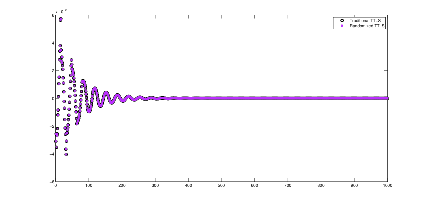
Refer to caption
Figure 1: Computed solutions for the true Tls solution and the randomized one.

5.2.3 Algorithm Rttls on ill-conditioned cases

Our ill-conditioned cases are taken from Hansen’s Regularizaton Tools [15]. For example, the case Shaw is generated by the command [A¯,b¯,xtrue]=Shaw(m)¯𝐴¯𝑏subscript𝑥trueShaw𝑚\left[\bar{A},~{}\bar{b},~{}x_{\mathrm{true}}\right]=\textsc{Shaw}(m). Then noises are added to A¯¯𝐴\bar{A} and b¯¯𝑏\bar{b}. Suppose that δ𝛿\delta is the relative noise level. We define

b=b¯+δb¯2ζζ2,A=A¯+δA¯FZZF,formulae-sequence𝑏¯𝑏𝛿subscriptnorm¯𝑏2𝜁subscriptnorm𝜁2𝐴¯𝐴𝛿subscriptnorm¯𝐴𝐹𝑍subscriptnorm𝑍𝐹\displaystyle b=\bar{b}+\delta\left\|\bar{b}\right\|_{2}\frac{\zeta}{\left\|\zeta\right\|_{2}},\qquad A=\bar{A}+\delta\left\|\bar{A}\right\|_{F}\frac{Z}{\|Z\|_{F}},

where ζ𝜁\zeta is a random vector, ζ=2rand(m,1)1𝜁2rand𝑚11\zeta=2*\mathrm{rand}(m,1)-1; Z𝑍Z is a random matrix, Z=2rand(m)1𝑍2rand𝑚1Z=2*\mathrm{rand}(m)-1. It is easy to verify that

bb¯2b¯2=AA¯FA¯F=δ.subscriptnorm𝑏¯𝑏2subscriptnorm¯𝑏2subscriptnorm𝐴¯𝐴𝐹subscriptnorm¯𝐴𝐹𝛿\frac{\left\|b-\bar{b}\right\|_{2}}{\left\|\bar{b}\right\|_{2}}=\frac{\left\|A-\bar{A}\right\|_{F}}{\left\|\bar{A}\right\|_{F}}=\delta.

Then we seek the total least squares solution of Axb𝐴𝑥𝑏Ax\approx b.

δ𝛿\delta k𝑘k TimeTtlssubscriptTimeTtls\mathrm{Time}_{\textsc{Ttls}} TimePtlssubscriptTimePtls\mathrm{Time}_{\textsc{Ptls}} TimeRttlssubscriptTimeRttls\mathrm{Time}_{\textsc{Rttls}} ErrRttlssubscriptErrRttls\mathrm{Err}_{\textsc{Rttls}}
1E-1 3 0.0123 0.2230 0.0039 8.04E-3
1E-2 5 0.0133 0.2365 0.0039 8.92E-4
1E-3 7 0.0119 0.2455 0.0075 1.59E-3
1E-4 8 0.0114 0.2424 0.0039 3.76E-4
Table 6: Tests on Shaw with different relative noise levels. The relative error ErrRttls=xrttlsxttls/xttlssubscriptErrRttlssubscriptnormsubscript𝑥rttlssubscript𝑥ttlssubscriptnormsubscript𝑥ttls\mathrm{Err}_{\textsc{Rttls}}=||x_{\textsc{rttls}}-x_{\textsc{ttls}}||_{\infty}/\|x_{\textsc{ttls}}\|_{\infty}. Algorithm Rttls is substantially faster than Ttls and Ptls.

We first test Algorithm Rttls on the 100×100100100100\times 100 matrix Shaw with different relative noise levels δ𝛿\delta. The results are given in Table 6. The truncation parameter k𝑘k is estimated by the randomized algorithm with Gcv and Tsvd [42]. After the determination of parameter k𝑘k, the computational time for implementing Algorithm Ttls and Algorithm Rttls is recorded in TimeTtlssubscriptTimeTtls\mathrm{Time}_{\textsc{Ttls}} and TimeRttlssubscriptTimeRttls\mathrm{Time}_{\textsc{Rttls}} respectively. And TimePtlssubscriptTimePtls\mathrm{Time}_{\textsc{Ptls}} denotes the time cost in Ttls using Lanczos bi-diagonalization based partial Svd. Here we denote the relative error ErrRttls=xttlsxrttls/xttls.subscriptErrRttlssubscriptnormsubscript𝑥ttlssubscript𝑥rttlssubscriptnormsubscript𝑥ttls\mathrm{Err}_{\textsc{Rttls}}=||x_{\textsc{ttls}}-x_{\textsc{rttls}}||_{\infty}/\|x_{\textsc{ttls}}\|_{\infty}. From our computing, we see that the computed solutions of Algorithm Ptls are almost the same as those of Algorithm Ttls, and hence the relative errors for the solutions of Ptls which we denote as ErrPtls=xptlsxttls/xttlssubscriptErrPtlssubscriptnormsubscript𝑥ptlssubscript𝑥ttlssubscriptnormsubscript𝑥ttls\mathrm{Err}_{\textsc{Ptls}}=\|x_{\textsc{ptls}}-x_{\textsc{ttls}}\|_{\infty}/\|x_{\textsc{ttls}}\|_{\infty} are much smaller. Here we ignore the error ErrPtlssubscriptErrPtls\mathrm{Err}_{\textsc{Ptls}} and do not list it in the table. From this table we can see that the results of Algorithm Rttls are very close to those of traditional Ttls even for the relative noise level as large as 10%. According to the computational time, Algorithm Ptls does not show obvious advantages over Ttls for small size cases, while Algorithm Rttls is substantially faster than the traditional Ttls. The computed solutions for the case where the relative noise level δ𝛿\delta=1E-3 are presented in Figure 2.

Refer to caption
Figure 2: Computed solutions for the case Shaw of size m𝑚m=100 with relative noise level δ𝛿\delta=1E-3.

We then test Algorithm Rttls on larger matrices. We set the parameter for sampling size l=10𝑙10l=10 and the relative noise level δ𝛿\delta=1E-3 for all cases. The results are given in Table 7. The marker * in Table 7 means we cannot load the example I_Laplace on our computer when the size n=5000.𝑛5000n=5000. Obviously, Ptls can be much faster than the Ttls when the size of the matrix becomes larger. But it is still not as efficient as the randomized one because of its Blas-2 operations. The randomized strategy can greatly speed up the classical Algorithm Ttls. The advantage of our Algorithm Rttls is more obvious when we test the larger matrices. The plots of the computed solutions are given in Figure 3.

Matrix size k𝑘k TimeTtlssubscriptTimeTtls\mathrm{Time}_{\textsc{Ttls}} TimePtlssubscriptTimePtls\mathrm{Time}_{\textsc{Ptls}} TimeRttlssubscriptTimeRttls\mathrm{Time}_{\textsc{Rttls}} ErrRttlssubscriptErrRttls\mathrm{Err}_{\textsc{Rttls}}
Baart m=100𝑚100m=100 4 0.0153 0.2907 0.0040 6.43E-3
m=1000𝑚1000m=1000 4 1.7561 0.2664 0.0143 6.53E-3
m=5000𝑚5000m=5000 4 176.47 1.5042 0.2471 5.86E-3
Deriv2 m=100𝑚100m=100 6 0.0130 0.2604 0.0040 1.39E-2
m=1000𝑚1000m=1000 7 1.6727 0.3589 0.0148 6.96E-2
m=5000𝑚5000m=5000 9 170.40 1.8398 0.2506 1.20E-2
Foxgood m=100𝑚100m=100 2 0.0129 0.2691 0.0037 4.60E-6
m=1000𝑚1000m=1000 3 1.7638 0.2795 0.0143 5.09E-4
m=5000𝑚5000m=5000 3 171.88 1.1383 0.2227 1.14E-4
Gravity m=100𝑚100m=100 7 0.0152 0.4679 0.0039 1.91E-3
m=1000𝑚1000m=1000 8 1.7214 0.2963 0.0147 6.70E-3
m=5000𝑚5000m=5000 9 183.92 2.2156 0.3014 3.16E-2
Heat m=100𝑚100m=100 8 0.0107 0.2283 0.0041 7.33E-2
m=1000𝑚1000m=1000 9 1.7172 0.3963 0.0163 3.93E-2
m=5000𝑚5000m=5000 9 165.56 1.4494 0.2551 8.15E-2
I_Laplace m=100𝑚100m=100 8 0.0182 0.2972 0.0056 2.22E-4
m=1000𝑚1000m=1000 9 3.4499 0.5609 0.0410 1.83E-2
m=5000𝑚5000m=5000 * * * * *
Phillips m=100𝑚100m=100 7 0.0109 0.2476 0.0038 1.66E-3
m=1000𝑚1000m=1000 7 2.3627 0.2804 0.0137 2.24E-3
m=5000𝑚5000m=5000 7 174.74 1.1844 0.2194 6.08E-3
Table 7: Algorithm Rttls on ill-conditioned cases.
Refer to caption
(a) Baart
Refer to caption
(b) Deriv2
Refer to caption
(c) Foxgood
Refer to caption
(d) Gravity
Refer to caption
(e) Heat
Refer to caption
(f) i_Laplace
Refer to caption
(g) Phillips
Refer to caption
(h) Shaw
Figure 3: Rttls for ill-conditioned cases of size m=1000𝑚1000m=1000 with relative noise level δ𝛿\delta=1E-3.

5.2.4 Test on Adaptive Algorithm Arttls

We still use the examples from Hansen’s Regularizaton Tools [15] and test the case with matrix size m=n=1000.𝑚𝑛1000m=n=1000. Here we set r=7𝑟7r=7 in the Algorithm Arttls. Different tolerances generate different j𝑗j’s in Algorithm Arttls. So we tried several ϵitalic-ϵ\epsilon’s to make sure that k𝑘k’s in Algorithm Rttls and j𝑗j’s in Algorithm Arttls are close, and then the comparisons for the relative errors and time are reasonable. The performance for Algorithm Arttls is shown in Table 8. In the table, ErrArttlssubscriptErrArttls\mathrm{Err}_{\textsc{Arttls}} denotes the relative error xttlsxarttls/xttlssubscriptnormsubscript𝑥ttlssubscript𝑥arttlssubscriptnormsubscript𝑥ttls||x_{\textsc{ttls}}-x_{\textsc{arttls}}||_{\infty}/\|x_{\textsc{ttls}}\|_{\infty} and TimeArttlssubscriptTimeArttls\mathrm{Time}_{\textsc{Arttls}} represents the time cost for Algorithm Arrtls. It is clear that Algorithm Arttls can still give good accuracy with less computational time than the traditional one under the fixed precision.

k𝑘k ϵitalic-ϵ\epsilon j𝑗j TimePtlssubscriptTimePtls\mathrm{Time}_{\textsc{Ptls}} TimeRttlssubscriptTimeRttls\mathrm{Time}_{\textsc{Rttls}} TimeArttlssubscriptTimeArttls\mathrm{Time}_{\textsc{Arttls}} ErrRttlssubscriptErrRttls\mathrm{Err}_{\textsc{Rttls}} ErrArttlssubscriptErrArttls\mathrm{Err}_{\textsc{Arttls}}
Baart 4 8E-1 4 0.4970 0.0266 0.0567 2.22E-2 4.24E-2
Deriv2 7 2E-2 8 0.4062 0.0223 0.0335 4.39E-2 1.45E-1
Foxgood 3 5E-1 3 0.3086 0.0206 0.0302 3.48E-4 2.14E-3
Gravity 8 7E-1 8 0.3449 0.0246 0.0436 5.66E-3 9.82E-3
Heat 9 4E-1 8 0.3412 0.0275 0.0383 2.08E-1 7.03E-2
I_Laplace 9 7E-1 10 0.6054 0.0408 0.1226 5.38E-3 7.07E-2
Phillips 7 4E-0 8 0.3218 0.0213 0.0367 1.44E-3 7.80E-3
Shaw 7 6E-1 7 0.6624 0.0330 0.0487 3.40E-3 1.03E-2
Table 8: Algorithm Arttls on ill-conditioned cases. The relative errors ErrRttls=xrttlsxttls/xttlssubscriptErrRttlssubscriptnormsubscript𝑥rttlssubscript𝑥ttlssubscriptnormsubscript𝑥ttls\mathrm{Err}_{\textsc{Rttls}}=||x_{\textsc{rttls}}-x_{\textsc{ttls}}||_{\infty}/\|x_{\textsc{ttls}}\|_{\infty}, ErrArttls=xttlsxarttls/xttlssubscriptErrArttlssubscriptnormsubscript𝑥ttlssubscript𝑥arttlssubscriptnormsubscript𝑥ttls\mathrm{Err}_{\textsc{Arttls}}=\|x_{\textsc{ttls}}-x_{\textsc{arttls}}\|_{\infty}/\|x_{\textsc{ttls}}\|_{\infty}. Both Rttls and Arttls need less computational time than Ptls based on Lanczos procedure.

6 Conclusion

In this paper, we derive a new perturbation bound for the total least squares problem. This sharper and numerically computable perturbation bound is well illustrated by the numerical examples. Also we show that three kinds of condition numbers in [2, 24, 44] obtained through different ways are mathematically equivalent. We propose randomized algorithms Rtls, Rttls and Arttls for the numerical solutions of well-conditioned and ill-conditioned total least squares problems, respectively. These randomized algorithms can greatly reduce the computational time, and still give solutions with good accuracy. The regularization parameter in Rttls is estimated by the truncated parameter of the Tsvd solution of Axb𝐴𝑥𝑏Ax\approx b based on a fast randomized Svd of A𝐴A [42]. Then a randomized Svd of [A,b]𝐴𝑏[A,b] together with this truncation parameter yields a good approximate Ttls solutions to the large-scale ill-conditioned total least squares problems. The detailed investigation on other regularization parameter choices, and other techniques such as Tikhonov regularization, will be our future research.

7 Acknowledgments

The authors would like to thank Marc Baboulin, Ken Hayami, Zhongxiao Jia, Lothar Reichel, and Jun Zou for their comments and suggestions which led to improvements of our manuscript.

References

  • [1] Blendenpik: Supercharging LAPACK’s least-squares solver, Avron, Haim and Maymounkov, Petar and Toledo, Sivan, SIAM J. Sci. Comput., Vol. 32, No. 3, pp. 1217–1236.
  • [2] Baboulin, Marc and Gratton, Serge, A contribution to the conditioning of the total least-squares problem, SIAM J. Matrix Anal. Appl., Vol. 32, 2011, No. 3, pp. 685–699.
  • [3] Baboulin, Marc and Gratton, Serge and Lacroix, Rémi and Laub, Alan, Efficient computation of condition estimates for linear least squares problems. To appear in the Proceedings of the 10th International Conference on Parallel Processing and Applied Mathematics, PPAM 2013(09/2013).
  • [4] Beck, Amir and Ben-Tal, Aharon, On the solution of the Tikhonov regularization of the total least squares problem, SIAM J. Optim., Vol. 17, 2006, No. 1, pp. 98–118.
  • [5] Beck, Amir and Ben-Tal, Aharon and Teboulle, Marc, Finding a global optimal solution for a quadratically constrained fractional quadratic problem with applications to the regularized total least squares, SIAM J. Matrix Anal. Appl., Vol. 28, 2006, No. 2, pp. 425–445.
  • [6] Chang, X.-W. and Titley-Peloquin, D., Backward perturbation analysis for scaled total least-squares problems, Numer. Linear Algebra Appl., Vol. 16, 2009, No. 8, pp. 627–648.
  • [7] De Moor, Bart and David, Johan, Total linear least squares and the algebraic Riccati equation, Systems Control Lett., Vol. 18, 1992, No. 5, pp. 329–337.
  • [8] Diao, Huaian and Shi, Xinghua and Wei, Yimin, Effective condition numbers and small sample statistical condition estimation for the generalized Sylvester equation, Sci. China Math., Vol. 56, 2013, No. 5, pp. 967–982.
  • [9] Fierro, R. D. and Golub, G. H. and Hansen, P. C. and O’Leary, D. P., Regularization by truncated total least squares, SIAM J. Sci. Comput., Vol. 18, 1997, No. 4, pp. 1223–1241.
  • [10] Golub, Gene H. and Hansen, Per Christian and O’Leary, Dianne P., Tikhonov regularization and total least squares, SIAM J. Matrix Anal. Appl., Vol. 21, 1999, No. 1, pp. 185–194 .
  • [11] Golub, Gene H. and Van Loan, Charles F., An analysis of the total least squares problem, SIAM J. Numer. Anal., Vol. 17, 1980, No. 6, pp. 883–893.
  • [12] Golub, Gene H. and Van Loan, Charles F., Matrix Computations, Johns Hopkins Studies in the Mathematical Sciences, 4th, Johns Hopkins University Press, Baltimore, MD, 2013, pp. xxx+698.
  • [13] Gratton, Serge and Titley-Peloquin, David and Ilunga, Jean Tshimanga, Sensitivity and conditioning of the truncated total least squares solution, SIAM J. Matrix Anal. Appl., Vol. 34, 2013, No. 3, pp. 1257–1276.
  • [14] Halko, N. and Martinsson, P. G. and Tropp, J. A., Finding structure with randomness: probabilistic algorithms for constructing approximate matrix decompositions, SIAM Rev., Vol. 53, 2011, No. 2, pp. 217–288.
  • [15] Hansen, Per Christian, Regularization tools: a Matlab package for analysis and solution of discrete ill-posed problems, Numer. Algorithms, Vol. 6, 1994, No. 1-2, pp. 1–35.
  • [16] Hansen, Per Christian and Nagy, James G and O’leary, Dianne P, Deblurring Images: Matrices, Spectra, and Filtering, Vol. 3, 2006, Society for Industrial and Applied Mathematics, Philadelphia.
  • [17] Hnětynková, Iveta and Plešinger, Martin and Sima, Diana Maria and Strakoš, Zdeněk and Van Huffel, Sabine, The total least squares problem in AXB𝐴𝑋𝐵AX\approx B: a new classification with the relationship to the classical works, SIAM J. Matrix Anal. Appl., Vol. 32, 2011, No. 3, pp. 748–770.
  • [18] Jia, Zhongxiao and Li, Bingyu, On the condition number of the total least squares problem, Numer. Math., Vol. 125, 2013, No. 1, pp. 61–87.
  • [19] Kenney, C. S. and Laub, A. J., Small-sample statistical condition estimates for general matrix functions, SIAM J. Sci. Comput., Vol. 15, 1994, No. 1, pp. 36–61.
  • [20] Kenney, C. S. and Laub, A. J. and Reese, M. S., Statistical condition estimation for linear least squares, SIAM J. Matrix Anal. Appl., Vol. 19, 1998, No. 4, pp. 906–923.
  • [21] Lampe, J. and Voss, H., Global convergence of RTLSQEP: a solver of regularized total least squares problems via quadratic eigenproblems, Math. Model. Anal., Vol. 13, 2008, No. 1, pp. 55–66.
  • [22] Lampe, Jörg and Voss, Heinrich, Large-scale Tikhonov regularization of total least squares, J. Comput. Appl. Math., Vol. 238, 2013, pp. 95–108.
  • [23] Lee, Geunseop and Fu, Haoying and Barlow, Jesse L, Fast High-Resolution Image Reconstruction Using Tikhonov Regularization Based Total Least Squares, SIAM J. Sci. Comput., Vol. 35, No. 1, pp. B275–B290, 2013.
  • [24] Li, Bingyu and Jia, Zhongxiao, Some results on condition numbers of the scaled total least squares problem, Linear Algebra Appl., Vol. 435, 2011, No. 3, pp. 674–686.
  • [25] Li, Zi-Cai and Chien, Cheng-Sheng and Huang, Hung-Tsai, Effective condition number for finite difference method, J. Comput. Appl. Math., Vol. 198, 2007, No. 1, pp. 208–235.
  • [26] Li, Zi-Cai and Huang, Hung-Tsai and Chen, Jeng-Tzong and Wei, Yimin, Effective condition number and its applications, Computing, Vol. 89, 2010, No. 1-2, pp. 87–112.
  • [27] Li, Zi-Cai and Huang, Hung-Tsai and Wei, Yimin, Ill-conditioning of the truncated singular value decomposition, Tikhonov regularization and their applications to numerical partial differential equations, Numer. Linear Algebra Appl., Vol. 18, 2011, No. 2, pp. 205–221.
  • [28] Liu, Xin-Guo, Solvability and perturbation analysis of the total least squares problem, Acta Math. Appl. Sinica, Vol. 19, 1996, No. 2, pp. 254–262.
  • [29] Lu, Shuai and Pereverzev, Sergei V. and Tautenhahn, Ulrich, Regularized total least squares: computational aspects and error bounds, SIAM J. Matrix Anal. Appl., Vol. 31, 2009, No. 3, pp. 918–941.
  • [30] Majda, George and Strauss, Walter A. and Wei, Musheng, Computation of exponentials in transient data, IEEE Transactions on Antennas and Propagation, 37 (1989), pp. 1284 C1290.
  • [31] Markovsky, Ivan and Rastello, Maria Luisa and Premoli, Amedeo and Kukush, Alexander and Van Huffel, Sabine, The element-wise weighted total least-squares problem, Comput. Statist. Data Anal., Vol. 50, 2006, No. 1, pp. 181–209.
  • [32] Malyshev, A. N., A unified theory of conditioning for linear least squares and Tikhonov regularization solutions, SIAM J. Matrix Anal. Appl., Vol. 24, 2003, No. 4, pp. 1186–1196.
  • [33] Paige, Christopher C. and Strakoš, Zdeněk, Scaled total least squares fundamentals, Numer. Math., Vol. 91, 2002, No. 1, pp. 117–146.
  • [34] Rahman, MD and Yu, Kai-Bor, Total least squares approach for frequency estimation using linear prediction, IEEE Transactions on Acoustics, Speech and Signal Processing, 35 (1987), pp. 1440-1454.
  • [35] Renaut, Rosemary A. and Guo, Hongbin, Efficient algorithms for solution of regularized total least squares, SIAM J. Matrix Anal. Appl., Vol. 26, 2004, No. 2, pp. 457–476.
  • [36] Sima, Diana M. and Van Huffel, Sabine and Golub, Gene H., Regularized total least squares based on quadratic eigenvalue problem solvers, BIT, Vol. 44, 2004, No. 4, pp. 793–812.
  • [37] Stewart, G. W., A second order perturbation expansion for small singular values, Linear Algebra Appl., Vol. 56, 1984, pp. 231–235.
  • [38] Van Huffel, Sabine and Vandewalle, Joos, The Total Least Squares Problem, Frontiers in Applied Mathematics, Vol. 9, Society for Industrial and Applied Mathematics (SIAM), Philadelphia, PA, 1991, pp. xiv+300.
  • [39] Wei, Musheng, The analysis for the total least squares problem with more than one solution, SIAM J. Matrix Anal. Appl., Vol. 13, 1992, No. 3, pp. 746–763.
  • [40] Wei, Musheng, Algebraic relations between the total least squares and least squares problems with more than one solution, Numer. Math., Vol. 62, 1992, No. 1, pp. 123–148.
  • [41] Wei, Musheng and Majda, George, A new theoretical approach for Prony’s method, Linear Algebra Appl., 136(1990), pp.119-132.
  • [42] Xiang, Hua and Zou, Jun, Regularization with randomized SVD for large-scale discrete inverse problems, Inverse Problems, Vol. 29, 2013, No. 8, pp. 085008, 23.
  • [43] Xu, Wei and Qiao, Sanzheng and Wei, Yimin, A note on the scaled total least squares problem, Linear Algebra Appl., Vol. 428, 2008, No. 2-3, pp. 469–478.
  • [44] Zhou, Liangmin and Lin, Lijing and Wei, Yimin and Qiao, Sanzheng, Perturbation analysis and condition numbers of scaled total least squares problems, Numer. Algorithms, Vol. 51, 2009, No. 3, pp. 381–399.