Nonconvex bundle method with application to a delamination problem

Abstract.

Delamination is a typical failure mode of composite materials caused by weak bonding. It arises when a crack initiates and propagates under a destructive loading. Given the physical law characterizing the properties of the interlayer adhesive between the bonded bodies, we consider the problem of computing the propagation of the crack front and the stress field along the contact boundary. This leads to a hemivariational inequality, which after discretization by finite elements we solve by a nonconvex bundle method, where upper-$C^{1}$ criteria have to be minimized. As this is in contrast with other classes of mechanical problems with non-monotone friction laws and in other applied fields, where criteria are typically lower-$C^{1}$, we propose a bundle method suited for both types of nonsmoothness. We prove its global convergence in the sense of subsequences and test it on a typical delamination problem of material sciences.

Key words. Composite material $\cdot$ delamination $\cdot$ crack front propagation $\cdot$ hemivariational inequality $\cdot$ Clarke directional derivative $\cdot$ nonconvex bundle method $\cdot$ lower- and upper-$C^{1}$ function $\cdot$ convergence.

1. Introduction

We develop a bundle technique to solve nonconvex variational problems arising in contact mechanics and in other applied fields. We are specifically interested in the delamination of composite structures with an adhesive bonding under destructive loading, a failure mode which is studied in the material sciences. When the properties of the interlayer adhesive between the bonded bodies are given in the form of a physical law relating the normal component of the stress vector to the relative displacement between the upper and lower boundaries at the crack tip, the challenge is to compute the displacement and stress fields in order to assess the reactive destructive forces along the contact boundary, as the latter are difficult to measure in situ. This leads to minimization of an energy functional, where a specific form of nonsmoothness arises in the boundary integral at the contact boundary. After discretization via piecewise linear finite elements using the trapezoidal quadrature rule, this leads to a finite-dimensional nonsmooth optimization problem of the form

(3) $$\begin{array}[]{ll}\mbox{minimize}&f(x)\\ \mbox{subject to}&Ax\leq b\end{array}$$

where $f$ is locally Lipschitz and neither smooth nor convex. Depending on the nature of the frictional forces, the criterion $f$ may be upper-$C^{1}$ or lower-$C^{1}$, see e.g. Figure 1. As these two classes of nonsmooth functions behave substantially differently when minimized, we are forced to expand on existing bundle strategies and develop an algorithm general enough to encompass both types of nonsmoothness. We prove its convergence to a critical point in the sense of subsequences, and show that it provides satisfactory numerical results in a simulation of the double cantilever beam test [1], one of the most popular destructive tests to qualify structural adhesive joints.

The difficulty in nonconvex bundling is to provide a suitable cutting plane oracle which replaces the no longer available convex tangent plane. One of the oldest oracles, discussed already in Mifflin [2], and used in the bundle codes of Lemaréchal and Sagastizábal [3, 4], or the BT-codes of Zowe [5, 6], uses the method of downshifted tangents. While these authors use linesearch with Armijo and Wolfe type conditions, which allows only weak convergence certificates in the sense that some accumulation point of the sequence of serious iterates is critical, we favor proximity control in tandem with a suitable backtracking strategy. This leads to stronger convergence certificates, where every accumulation point of the sequence of serious iterates is critical. For instance, in [7, 8, 9] a strong certificate for downshifted tangents with proximity control was proved within the class of lower-$C^{1}$ functions, but its validity for upper-$C^{1}$ criteria remained open. An oracle for upper-$C^{1}$ functions with a rigorous convergence theory can be based on the model approach of [7, 8, 10], but the latter is not compatible with the downshift oracle.

To have two strings to one bow is unsatisfactory, as one could hardly expect practitioners to select their strategy according to such a distinction, which might not be easy to make in practice. In this work we will resolve this impasse and present a cutting plane oracle based on downshifted tangents, which leads to a bundle method with strong convergence certificate for both types of nonsmoothness. In its principal components our method agrees with existing strategies for downshifted tangents, like [3, 5, 11, 12], and could therefore be considered as a justification of this technique for a wide class of applications. Differences with existing methods occur in the management of the proximity control parameter, which in our approach has to respect certain rules to assure convergence to a critical point, without impeding good practical performance.

The structure of the paper is as follows. Section 2 gives some preparatory information on lower- and upper-$C^{1}$ functions. Section 4 presents the algorithm and comments on its ingredients. Theoretical tools needed to prove convergence are presented and employed in sections 3 and 5. Section 6 gives the main convergence result, while section 7 discusses practical aspects of the algorithm. In section 8, we discuss the delamination problem, which we solve numerically using our bundle algorithm.

Numerical results for contact problem with adhesion based on the bundle-Newton method of L. Lukšan and J. Vlček [13] can be found e.g. in the book of Haslinger et al. [14], in [11, 12], and in the more recent [15, 16]. Mathematical analysis and numerical results for quasistatic delamination problems can be found in [17, 18].

2. Lower- and upper-$C^{1}$ functions

Following Spingarn [19], a locally Lipschitz function $f:\mathbb{R}^{n}\to\mathbb{R}$ is lower-$C^{1}$ at $x_{0}$, if there exists a compact Hausdorff space $K$, a neighborhood $U$ of $x_{0}$, and a mapping $F:U\times K\to\mathbb{R}$ such that both $F$ and $D_{x}F$ are jointly continuous and

(4) $$f(x)=\max\{F(x,y):y\in K\}$$

is satisfied for $x\in U$. The function $f$ is upper-$C^{1}$ at $x_{0}$ if $-f$ is lower-$C^{1}$ at $x_{0}$.

In a minimization problem (3), we expect lower- and upper-$C^{1}$ functions to behave completely differently. Minimizing a lower-$C^{1}$ function ought to lead to real difficulties, as on descending we move into the zone of nonsmoothness, which for lower-$C^{1}$ goes downward. In contrast, upper-$C^{1}$ functions are generally expected to be well-behaved, as intuitively on descending we move away from the nonsmoothness, which here goes upward. The present application shows that this argument is too simplistic. Minimization of upper-$C^{1}$ functions leads to real difficulties, which we explain subsequently. In delamination for composite materials we encounter objective functions of the form

(5) $$f(x)=f_{s}(x)+\int_{0}^{1}\min_{i\in I}f_{i}(x,t)\,dt,$$

where $f_{s}$ gathers the smooth part, while the integral term, due to the minimum, is responsible for the nonsmoothness.

Lemma 1.

Suppose $f_{s}$ is of class $C^{1}$ and the $f_{i}$ are jointly of class $C^{1}$. Then the function (5) is upper-$C^{1}$ and can be represented in the form

(6) $$f(x)=f_{s}(x)+\min_{\sigma\in\Sigma}\int_{0}^{1}f_{\sigma(t)}(x,t)\,dt,$$

where $\Sigma$ is the set of all measurable mappings $\sigma:[0,1]\to I$.

Proof.

Let us first prove (6). For $\sigma\in\Sigma$ and fixed $x\in\mathbb{R}^{n}$ the function $t\mapsto f_{\sigma(t)}(x,t)$ is measurable, and since $\min_{i\in I}f_{i}(x,t)\leq f_{\sigma(t)}(x,t)\leq\max_{i\in I}f_{i}(x,t)$, it is also integrable. Hence $F(x,\sigma)=f_{s}(x)+\int_{0}^{1}f_{\sigma(t)}(x,t)\,dt$ is well-defined, and clearly $F(x,\sigma)\geq f(x)$, so we have $\inf_{\sigma\in\Sigma}F(x,\sigma)\geq f(x)$.

To prove the reverse estimate, fix $x\in\mathbb{R}^{n}$ and consider the closed-valued multifunction $\Phi:[0,1]\to 2^{I}$ defined by $\Phi(t)=\{i\in I:f_{i}(x,t)=\min_{i^{\prime}\in I}f_{i^{\prime}}(x,t)\}$. Since the $f_{i}(x,\cdot)$ are measurable and $I$ is finite, $\Phi$ is a measurable multifunction. Choose a measurable selection $\sigma$, that is, $\sigma\in\Sigma$ satisfying $\sigma(t)\in\Phi(t)$ for every $t\in[0,1]$. Then clearly $F(x,\sigma)=f(x)$. This proves (6).

Let us now show that $f$ is upper-$C^{1}$. We consider $\varphi(x,t)=\min_{i\in I}f_{i}(x,t).$ In view of [19] $\varphi(\cdot,t)$ is upper-$C^{1}$ and its Clarke subdifferential $\partial\varphi(\cdot,t)$ is strictly supermonotone uniformly over $t\in[0,1]$. By Theorem 2 in [20], $\varphi(\cdot,t)$ is approximately concave uniformly over $t\in[0,1]$. Integration with respect to $t\in[0,1]$ then yields an approximately concave function with respect to $x$, which by the equivalences in [20] and [19] is upper-$C^{1}$. ∎

Note that the minimum (6) is semi-infinite even though $I$ is finite. Minimization of (5) cannot be converted into a NLP, as would be possible in the min-max case. The representation (6) highlights the difficulty in minimizing (5). Minimizing a minimum has a disjunctive character, and due to the large size of $\Sigma$ this could lead to a combinatorial situation with intrinsic difficulty.

3. The model concept

The model of a nonsmooth function was introduced in [8] and is a key element in understanding the bundle concept.

Definition 1 (Compare [8]).

A function $\phi:\mathbb{R}^{n}\times\mathbb{R}^{n}\to\mathbb{R}$ is called a model of the locally Lipschitz function $f:\mathbb{R}^{n}\to\mathbb{R}$ on the set $\Omega\subset\mathbb{R}^{n}$ if the following axioms are satisfied:

1. For every $x\in\Omega$ the function $\phi(\cdot,x):\mathbb{R}^{n}\to\mathbb{R}$ is convex, $\phi(x,x)=f(x)$ and $\partial_{1}\phi(x,x)\subset\partial f(x)$.

2. For every $x\in\Omega$ and every $\epsilon>0$ there exists $\delta>0$ such that $f(y)\leq\phi(y,x)+\epsilon\|y-x\|$ for every $y\in B(x,\delta)$.

3. The function $\phi$ is jointly upper semicontinuous, i.e., $(y_{j},x_{j})\to(y,x)$ on $\mathbb{R}^{n}\times\Omega$ implies $\displaystyle\limsup_{j\to\infty}\phi(y_{j},x_{j})\leq\phi(y,x)$. $\square$

We recall that every locally Lipschitz function $f$ has the so-called standard model

$$\phi^{\sharp}(y,x)=f(x)+f^{0}(x,y-x),$$

where $f^{0}(x,d)$ is the Clarke directional derivative of $f$ at $x$ in direction $d$. The same function $f$ may in general have several models $\phi$, and following [7, 10], the standard $\phi^{\sharp}$ is the smallest one. Every model $\phi$ gives rise to a bundle strategy. The question is then whether this bundle strategy is successful. This depends on the following property of $\phi$.

Definition 2.

A model $\phi$ of $f$ on $\Omega$ is said to be strict at $x_{0}\in\Omega$ if axiom $(M_{2})$ is replaced by the stronger

1. For every $\epsilon>0$ there exists $\delta>0$ such that $f(y)\leq\phi(y,x)+\epsilon\|y-x\|$ for all $x,y\in B(x_{0},\delta)$.

We say that $\phi$ is a strict model on $\Omega$, if it is strict at every $x_{0}\in\Omega$. $\square$

Remark 1.

We may write axiom $(M_{2})$ in the form $f(y)\leq\phi(y,x_{0})+{\rm o}(\|y-x_{0}\|)$ for $y\to x_{0}$, and $(\widehat{M}_{2})$ as $f(y)\leq\phi(y,x)+{\rm o}(\|y-x\|)$ for $x,y\to x_{0}$. Except for the fact that these concepts are one-sided, this is precisely the difference between differentiability and strict differentiability. Hence the nomenclature.

Lemma 2 (Compare [7, 10]).

Suppose $f$ is upper-$C^{1}$. Then its standard model $\phi^{\sharp}$ is strict, and hence every model $\phi$ of $f$ is strict. $\square$

Remark 2.

For convex $f$ the standard model $\phi^{\sharp}$ is in general not strict, but $f$ may be used as its own model $\phi(\cdot,x)=f$. For nonconvex $f$, a wide range of applications is covered by composite functions $f=g\circ F$ with $g$ convex and $F$ differentiable. Here the so-called natural model $\phi(y,x)=g(F(x)+F^{\prime}(x)(y-x))$ can be used, because it is strict as soon as $F$ is class $C^{1}$. This includes lower-$C^{2}$ functions in the sense of [21], lower-$C^{1,\alpha}$ functions in the sense of [22], or amenable functions in the sense of [23], which allow representations of the form $f=g\circ F$ with $F$ of class $C^{1,1}$.

We conclude with the remark that lower-$C^{1}$ functions also admit strict models, even though in that case the construction is more delicate. The strict model in that case cannot be exploited algorithmically, and for lower-$C^{1}$ functions we prefer the oracle concept, which will be discussed in section 5.

4. Elements of the algorithm

In this section we briefly explain the main features of the algorithm. This concerns building the working model, computing the solution of the tangent program, checking acceptance, updating the working model after null steps, and the management of the proximity control parameter.

4.1. Working model

At the current serious iterate $x$ the inner loop of the algorithm at counter $k$ computes an approximation $\phi_{k}(\cdot,x)$ of $f$ in a neighborhood of $x$, called a first-order working model. The working model is a polyhedral convex function of the form

(7) $$\phi_{k}(\cdot,x)=\max_{(a,g)\in\mathcal{G}_{k}}a+g^{\top}(\cdot-x),$$

where $\mathcal{G}_{k}$ is a finite set of affine functions $y\mapsto a+g^{\top}(y-x)$ satisfying $a\leq f(x)$, referred to as planes. The set $\mathcal{G}_{k}$ is updated during the inner loop $k$. At each step $k$ the following rules have to be respected when updating $\mathcal{G}_{k}$ into $\mathcal{G}_{k+1}$:

1. One or several cutting planes at the null step $y^{k}$, generated by an abstract cutting plane oracle, are added to $\mathcal{G}_{k+1}$.

2. The so-called aggregate plane $(a^{*},g^{*})$, which consists of convex combinations of elements of $\mathcal{G}_{k}$, is added to $\mathcal{G}_{k+1}$.

3. Some older planes in $\mathcal{G}_{k}$, which become obsolete through the addition of the aggregate plane, are discarded and not kept in $\mathcal{G}_{k+1}$.

4. Every $\mathcal{G}_{k}$ contains at least one so-called exactness plane $(a_{0},g_{0})$, where exactness plane means $a_{0}=f(x)$, $g_{0}\in\partial f(x)$. This assures $\phi_{k}(x,x)=f(x)$, hence the name.

5. We have to make sure that each working model $\phi_{k}$ satisfies $\partial_{1}\phi_{k}(x,x)\subset\partial f(x)$.

Once the first-order working model $\phi_{k}(\cdot,x)$ has been built, the second-order working model $\Phi_{k}(\cdot,x)$ is of the form

(8) $$\Phi_{k}(\cdot,x)=\phi_{k}(\cdot,x)+\textstyle\frac{1}{2}(\cdot-x)^{\top}Q(x)(\cdot-x),$$

where $Q(x)=Q(x)^{\top}$ is a possibly indefinite symmetric matrix, depending only on the current serious iterate $x$, and fixed during the inner loop $k$. The second-order term includes curvature information on $f$, if available.

4.2. Tangent program and acceptance test

Once the second-order working model (8) is formed and the proximity control parameter $\tau_{k-1}\to\tau_{k}$ is updated, we solve the tangent program

(11) $$\begin{array}[]{ll}\mbox{minimize}&\Phi_{k}(y,x)+\frac{\tau_{k}}{2}\|y-x\|^{2}\\ \mbox{subject to}&Ay\leq b\end{array}$$

Here the proximity control parameter $\tau_{k}$ satisfies $Q+\tau_{k}I\succ 0$, which assures that (11) is strictly convex and has a unique solution, $y^{k}$, called the trial step. The trial step is a candidate to become the new serious iterate $x^{+}$. In order to decide whether $y^{k}$ is acceptable, we compute the test

(12) $$\rho_{k}=\frac{f(x)-f(y^{k})}{f(x)-\Phi_{k}(y^{k},x)}\stackrel{{\scriptstyle?}}{{\geq}}\gamma,$$

where $0<\gamma<1$ is some fixed parameter. If $\rho_{k}\geq\gamma$, then $x^{+}=y^{k}$ is accepted and called a serious step. In this case the inner loop ends successfully. On the other hand, if $\rho_{k}<\gamma$, then $y^{k}$ is rejected and called a null step. In this case the inner loop $k$ continues. This means we will update working model $\Phi_{k}(\cdot,x)\to\Phi_{k+1}(\cdot,x)$, adjust the proximity control parameter $\tau_{k}\to\tau_{k+1}$, and solve (11) again.

Note that the test (12) corresponds to the usual Armijo descent condition used in linesearches, or to the standard acceptance test in trust region methods.

4.3. Updating the working model via aggregation

Suppose the trial step $y^{k}$ fails the acceptance test (12) and is declared a null step. Then the inner loop has to continue, and we have to improve the working model at the next sweep in order to perform better. Since the second-order part of the working model $\frac{1}{2}(\cdot-x)^{\top}Q(x)(\cdot-x)$ remains invariant, we will update the first-order part only.

Concerning rule $(R_{2})$, by the necessary optimality condition for (11), there exists a multiplier $\eta^{*}$ such that

$$0\in\partial_{1}\Phi_{k}(y^{k},x)+\tau_{k}(y^{k}-x)+A^{\top}\eta^{*},$$

or what is the same,

$$(Q(x)+\tau_{k}I)(y^{k}-x)-A^{\top}\eta^{*}\in\partial_{1}\phi_{k}(y^{k},x).$$

Since $\phi_{k}(\cdot,x)$ is by construction a maximum of affine planes, we use the standard description of the convex subdifferential of a max-function. Writing $\mathcal{G}_{k}=\{(a_{0},g_{0}),\dots,(a_{p},g_{p})\}$ for $p={\rm card}(\mathcal{G}_{k})+1$, we find non-negative multipliers $\lambda_{0},\dots,\lambda_{p}$ summing up to 1 such that

$$(Q(x)+\tau_{k}I)(y^{k}-x)-A^{\top}\eta^{*}=\sum_{i=0}^{p}\lambda_{i}g_{i},$$

and in addition, $a_{i}+g_{i}^{\top}(y^{k}-x)=\phi_{k}(y^{k},x)$ for all $i\in\{0,\dots,p\}$ with $\lambda_{i}>0$. We say that those planes which are active at $y^{k}$ are called by the aggregate plane. In the above rule $(R_{3})$ we allow those to be removed from $\mathcal{G}_{k}$. We now define the aggregate plane as:

$$a^{*}_{k}=\sum_{i=0}^{p}\lambda_{i}a_{i},\quad g^{*}_{k}=\sum_{i=0}^{p}\lambda_{i}g_{i}.$$

Note that by construction the aggregate plane $m_{k}^{*}(\cdot,x)=a^{*}_{k}+g^{*\top}_{k}(\cdot-x)$ at null step $y^{k}$ satisfies $m_{k}^{*}(y^{k},x)=a^{*}+g^{*\top}(y^{k}-x)=\phi_{k}(y^{k},x)$. This construction is standard and follows the original idea in Kiwiel [24]. It assures in particular that $\Phi_{k+1}(y^{k},x)\geq m_{k}^{*}(y^{k},x)+\frac{1}{2}(y^{k}-x)^{\top}Q(x)(y^{k}-x)=\Phi_{k}(y^{k},x)$.

4.4. Updating the working model by cutting planes and exactness planes

The crucial improvement in the first-order working model is in adding a cutting plane which cuts away the unsuccessful trial step $y^{k}$ according to rule $(R_{1})$. We shall denote the cutting plane as $m_{k}(\cdot,x)=a_{k}+g^{\top}(\cdot-x)$. The only requirement for the time being is that $a_{k}\leq f(x)$, as this assures $\phi_{k+1}(x,x)\leq f(x)$. Since we also maintain at least one exactness plane of the form $m_{0}(\cdot,x)=f(x)+g_{0}^{\top}(\cdot-x)$ with $g_{0}\in\partial f(x)$, we assure $\phi_{k+1}(x,x)=\Phi_{k+1}(x,x)=f(x)$. Later we will also have to check the validity of $(R_{5})$.

It is possible to integrate so-called anticipated cutting planes in the new working model $\mathcal{G}_{k+1}$. Here anticipated designates all planes which are not based on the rules exactness, aggregation, cutting planes. Naturally, adding such planes can not be allowed in an arbitrary way, because axioms $(R_{1})-(R_{5})$ have to be respected.

Remark 3.

It may be beneficial to choose a new exactness plane $m_{0}(\cdot,x)=f(x)+g^{\top}(\cdot-x)$ after each null step $y$, namely the one which satisfies $m_{0}(y,x)=f^{0}(x,y-x)$. If $x$ is a point of differentiability of $f$, then all these exactness planes are identical anyway, so no extra work occurs. On the other hand, computing $g\in\partial f(x)$ such that $g^{\top}(y-x)=f^{0}(x,y-x)$ is usually cheap. Consider for instance eigenvalue optimization, where $f(x)=\lambda_{1}\left(F(x)\right)$, $x\in\mathbb{R}^{n}$, $F:\mathbb{R}^{n}\to\mathbb{S}^{m}$, and $\lambda_{1}:\mathbb{S}^{m}\to\mathbb{R}$ is the maximum eigenvalue function of $\mathbb{S}^{m}$. Then $f^{0}(x,d)=\lambda_{1}^{\prime}(X,D)=\lambda_{1}(Q^{\top}DQ)$, where $X=F(x)$, $D=F^{\prime}(x)d$, and where $Q$ is a $t\times m$ matrix whose columns form an orthogonal basis of the maximum eigenspace of $X$ of dimension $t$ [25]. Then $G=QQ^{\top}\in\partial\lambda_{1}(X)$ attains $\lambda_{1}^{\prime}(X,D)$, hence $g=F^{\prime}(x)^{*}QQ^{\top}$ attains $f^{\prime}(x,d)$. Since usually $t\ll m$, the computation of $g$ is cheap.

4.5. Management of proximity control

The central novelty of the bundle methods developed in [7, 8, 26] is the discovery that in the absence of convexity the proximity control parameter $\tau$ has to follow certain basic rules to assure convergence of the sequence $x^{j}$ of serious iterates. This is in contrast with convex bundle methods, where $\tau$ could in principle be frozen once and for all. More precisely, suppose $\phi_{k}(\cdot,x)$ has failed and produced only a null step $y^{k}$. Having built the new model $\phi_{k+1}(\cdot,x)$, we compute the secondary test

(13) $$\widetilde{\rho}_{k}=\frac{f(x)-\Phi_{k+1}(y^{k},x)}{f(x)-\Phi_{k}(y^{k},x)}\stackrel{{\scriptstyle?}}{{\geq}}\widetilde{\gamma},$$

where $0<\gamma<\widetilde{\gamma}<1$ is fixed. Our decision is

(16) $$\tau_{k+1}=\left\{\begin{array}[]{ll}2\tau_{k}&\mbox{if }\widetilde{\rho}_{k}\geq\widetilde{\gamma}\\ \tau_{k}&\mbox{if }\widetilde{\rho}_{k}<\widetilde{\gamma}\end{array}\right.$$

The rationale of (13) is to decide whether improving the model by adding planes will suffice, or shorter steps have to be forced by increasing $\tau$.

The denominator in (13) gives the model predicted progress $f(x)-\phi_{k}(y^{k},x)=\phi_{k}(x,x)-\phi_{k}(y^{k},x)>0$ at $y^{k}$. On the other hand, the numerator $f(x)-\phi_{k+1}(y^{k},x)$ gives the progress over $x$ we would achieve at $y^{k}$, had we already known the cutting planes drawn at $y^{k}$. Due to aggregation we know that $\phi_{k+1}(y^{k},x)\geq\phi_{k}(y^{k},x)$, so that $\widetilde{\rho}_{k}\leq 1$, but values $\widetilde{\rho}_{k}\approx 1$ indicate that little to no progress is achieved by adding the cutting plane. In this case we decide that the $\tau$-parameter must be increased to force smaller steps, because that reinforces the agreement between $f$ and $\phi_{k+1}(\cdot,x)$.

In the test (16) we replace $\widetilde{\rho}_{k}\approx 1$ by $\widetilde{\rho}_{k}\geq\widetilde{\gamma}$ for some fixed $0<\gamma<\widetilde{\gamma}<1$. If $\widetilde{\rho}_{k}<\widetilde{\gamma}$, then the quotient if far from 1 and we decide that adding planes has still the potential to improve the situation. In that event we do not increase $\tau$.

Let us next consider the management of $\tau$ in the outer loop. Since $\tau$ can only increase or stay fixed in the inner loop, we allow $\tau$ to decrease between serious steps $x\to x^{+}$, respectively, $x^{j}\to x^{j+1}$. This is achieved by the test

(17) $${\rho}_{k_{j}}=\frac{f(x^{j})-f(x^{j+1})}{f(x^{j})-\Phi_{k_{j}}(x^{j+1},x^{j})}\stackrel{{\scriptstyle?}}{{\geq}}\Gamma,$$

where $0<\gamma\leq\Gamma<1$ is fixed. In other words, if at acceptance we have not only $\rho_{k_{j}}\geq\gamma$, but even $\rho_{k_{j}}\geq\Gamma$, then we decrease $\tau$ at the beginning of the next inner loop $j+1$, because we may trust the model. On the other hand, if $\gamma\leq\rho_{k_{j}}<\Gamma$ at acceptance, then we memorize the last $\tau$-parameter used, that is $\tau_{k_{j}}$ at the end of the $j$th inner loop.

Remark 4.

We should compare our management of the proximity control parameter $\tau$ with other strategies in the literature. For instance Mäkelä et al. [11] consider a very different management of $\tau$, which is motivated by the convex case.

4.6. Statement of the algorithm

We are now ready to give our formal statement of algorithm 1.

Algorithm 1 $\!\!{\bf.}$ Proximity control algorithm for (3).

 

0:  $0<\gamma<\Gamma<1$, $\gamma<\widetilde{\gamma}<1$, $0<q<\infty$, $q<T<\infty$.

1:  Initialize outer loop. Choose initial guess $x^{1}$ with $Ax^{1}\leq b$ and an initial matrix $Q_{1}=Q_{1}^{\top}$ with $-qI\preceq Q_{1}\preceq qI$. Fix memory control parameter $\tau_{1}^{\sharp}$ such that $Q_{1}+\tau_{1}^{\sharp}I\succ 0$. Put $j=1$.

2:  Stopping test. At outer loop counter $j$, stop if $0\in\partial f(x^{j})+A^{\top}\eta^{*}$ for some multiplier $\eta^{*}\geq 0$. Otherwise goto inner loop.

3:  Initialize inner loop. Put inner loop counter $k=1$ and initialize $\tau$-parameter using the memory element, i.e., $\tau_{1}=\tau^{\sharp}_{j}$. Choose initial convex working model $\phi_{1}(\cdot,x^{j})$, possibly recycling some planes from previous sweep $j-1$, and let $\Phi_{1}(\cdot,x^{j})=\phi_{1}(\cdot,x^{j})+\frac{1}{2}(\cdot-x^{j})^{\top}Q_{j}(\cdot-x^{j})$.

4:  Trial step generation. At inner loop counter $k$ solve tangent program

$$\min_{Ay\leq b}\Phi_{k}(y,x^{j})+\textstyle\frac{\tau_{k}}{2}\|y-x^{j}\|^{2}.$$

The solution is the new trial step $y^{k}$.

5:  Acceptance test. Check whether

$$\rho_{k}=\frac{f(x^{j})-f(y^{k})}{f(x^{j})-\Phi_{k}(y^{k},x^{j})}\geq\gamma.$$

If this is the case put $x^{j+1}=y^{k}$ (serious step), quit inner loop and goto step 8. If this is not the case (null step) continue inner loop with step 6.

6:  Update working model. Build new convex working model $\phi_{k+1}(\cdot,x^{j})$ based on null step $y^{k}$ by adding an exactness plane $m_{k}^{\sharp}(\cdot,x^{j})$ satisfying $m_{k}^{\sharp}(y^{k},x^{j})=f^{0}(x^{j},y^{k}-x^{j})$, a downshifted tangent $m_{k}^{\downarrow}(\cdot,x^{j})$, and the aggregate plane $m_{k}^{*}(\cdot,x^{j})$. Apply rule $(R_{3})$ to avoid overflow. Build $\Phi_{k+1}(\cdot,x^{j})$, and goto step 7.

7:  Update proximity parameter. Compute

$$\widetilde{\rho}_{k}=\frac{f(x^{j})-\Phi_{k+1}(y^{k},x^{j})}{f(x^{j})-\Phi_{k}(y^{k},x^{j})}.$$

Put

$$\tau_{k+1}=\left\{\begin{array}[]{ll}\vspace{.1cm}\tau_{k},&\mbox{if }\widetilde{\rho}_{k}<\widetilde{\gamma}\qquad\mbox{(bad)}\\ \vspace{.1cm}2\tau_{k},&\mbox{if }\widetilde{\rho}_{k}\geq\widetilde{\gamma}\qquad\mbox{(too bad)}\end{array}\right.$$

Then increase counter $k$ and continue inner loop with step 4.

8:  Update $Q_{j}$ and memory element. Update matrix $Q_{j}\to Q_{j+1}$, respecting $Q_{j+1}=Q_{j+1}^{\top}$ and $-qI\preceq Q_{j+1}\preceq qI$. Then store new memory element

$$\tau_{j+1}^{\sharp}=\left\{\begin{array}[]{ll}\tau_{k},&\mbox{if }\gamma\leq\rho_{k}<\Gamma\qquad\mbox{ (not bad)}\\ &\\ \displaystyle\textstyle\frac{{1}}{2}\tau_{k},&\mbox{if }\rho_{k}\geq\Gamma\qquad\qquad\mbox{ (good)}\end{array}\right.$$

Increase $\tau_{j+1}^{\sharp}$ if necessary to ensure $Q_{j+1}+\tau_{j+1}^{\sharp}I\succ 0$.

9:  Large multiplier safeguard rule. If $\tau_{j+1}^{\sharp}>T$ then re-set $\tau_{j+1}^{\sharp}=T$. Increase outer loop counter $j$ by 1 and loop back to step 2.

 

5. Nonconvex cutting plane oracles

In the convex cutting plane method [27, 28] unsuccessful trial steps $y^{k}$ are cut away by adding a tangent plane to $f$ at $y^{k}$ into the model. Due to convexity, the cutting plane is below $f$ and can therefore be used to construct an approximation (7) of $f$. For nonconvex $f$, cutting planes are more difficult to construct, but several ideas have been discussed. We mention [29, 2]. In [7] we have proposed an axiomatic approach, which has the advantage that it covers the applications we are aware of, and allows a convenient convergence theory. Here we use this axiomatic approach in the convergence proof.

Definition 3 (Compare [7]).

Let $f$ be locally Lipschitz. A cutting plane oracle for $f$ on the set $\Omega$ is an operator $\mathscr{O}$ which, with every pair $(x,y)$, $x$ a serious iterate in $\Omega$, $y\in\mathbb{R}^{n}$ a null step, associates an affine function $m_{y}(\cdot,x)=a+g^{\top}(\cdot-x)$, called the cutting plane at null step $y$ for serious iterate $x$, so that the following axioms are satisfied:

1. For $y=x$ we have $a=f(x)$ and $g\in\partial f(x)$.

2. Let $y_{j}\to x$. Then there exist $\epsilon_{j}\to 0^{+}$ such that $f(y_{j})\leq m_{y_{j}}(y_{j},x)+\epsilon_{j}\|y_{j}-x\|$.

3. Let $x_{j}\to x$ and $y_{j},y_{j}^{+}\to y$. Then there exists $z\in\mathbb{R}^{n}$ such that
   $\displaystyle\limsup_{j\to\infty}m_{y_{j}^{+}}(y_{j},x_{j})\leq m_{z}(y,x)$. $\square$

As we shall see, these axioms are aligned with the model axioms $(M_{1})-(M_{3})$. Not unexpectedly, there is also a strict version of $(O_{2})$.

Definition 4.

A cutting plane oracle $\mathscr{O}$ for $f$ is called strict at $x_{0}$ if the following strict version of $(O_{2})$ is satisfied:

1. Suppose $y_{j},x_{j}\to x$. Then there exist $\epsilon_{j}\to 0^{+}$ such that $f(y_{j})\leq m_{y_{j}}(y_{j},x_{j})+\epsilon_{j}\|y_{j}-x_{j}\|$. $\square$

We now discuss two versions of the oracle which are of special interest for our applications.

Example 5.1 (Model-based oracle).

Suppose $\phi$ is a model of $f$. Then we can generate a cutting plane for serious iterate $x$ and trial step $y$ by taking $g\in\partial_{1}\phi(y,x)$ and putting

$$m_{y}(\cdot,x)=\phi(y,x)+g^{\top}(\cdot-y)=\phi(y,x)+g^{\top}(x-y)+g^{\top}(\cdot-x).$$

Oracles generated by a model $\phi$ in this way will be denoted $\mathscr{O}_{\phi}$. Note that $\mathscr{O}_{\phi}$ coincides with the standard oracle if $f$ is convex and $\phi(\cdot,x)=f$, i.e., if the convex $f$ is chosen as its own model. In more general cases, the simple idea of this oracle is that in the absence of convexity, where tangents to $f$ at $y$ are not useful, we simply take tangents of $\phi(\cdot,x)$ at $y$. Note that the model-based oracle $\mathscr{O}_{\phi}$ is strict as soon as the model $\phi$ is strict. $\square$

Example 5.2 (Standard oracle).

A special case of the model-based oracle is obtained by choosing the standard model $\phi^{\sharp}$. Due to its significance for our present work we call this the standard oracle. The standard cutting plane for serious step $x$ and null step $y$ is $m_{y}^{\sharp}(\cdot,x)=f(x)+g^{\top}(\cdot-x)$, where the Clarke subgradient $g\in\partial f(x)$ is one of those that satisfy $g^{\top}(y-x)=f^{0}(x,y-x)$. The standard oracle is strict iff $\phi^{\sharp}$ is strict. As was observed before, this is for instance the case when $f$ is upper-$C^{1}$. Note a specificity of the standard oracle: every standard cutting plane $m_{y}^{\sharp}(\cdot,x)$ is also an exactness plane at $x$. $\square$

Example 5.3 (Downshifted tangents).

Probably the oldest oracle used for nonconvex functions are downshifted tangents, which we define as follows. For serious iterate $x$ and null step $y$ let $t(\cdot)=f(y)+g^{\top}(\cdot-y)$ be a tangent of $f$ at $y$. That is, $g\in\partial f(y)$. Then we shift $t(\cdot)$ down until it becomes useful for the model (7). Fixing a parameter $c>0$, this is organized as follows: We define the cutting plane as $m_{y}^{\downarrow}(\cdot,x)=t(\cdot)-s$, where the downshift $s\geq 0$ satisfies

$$s=[t(x)-f(x)+c\|y-x\|^{2}]_{+}.$$

In other words, $m_{y}^{\downarrow}(\cdot,x)=a+g^{\top}(\cdot-x)$, where $a=\min\{t(x),f(x)-c\|y-x\|^{2}\}$. Note that this procedure aways satisfies axioms $(O_{1})$ and $(O_{3})$, whereas axioms $(O_{2})$, respectively, $(\widehat{O}_{2})$, are satisfied if $f$ is lower-$C^{1}$ at $x_{0}$. In other words, see [7], for $f$ lower-$C^{1}$ this is an oracle, which is automatically strict. $\square$

Motivated by the previous examples, we now define an oracle which works for both lower-$C^{1}$ and upper-$C^{1}$.

Example 5.4 (Modified downshift).

Let $x$ be the current serious iterate, $y$ a null step in the inner loop belonging to $x$. Then we form the downshifted tangent $m_{y}^{\downarrow}(\cdot,x):=t(\cdot)-s$, that is, the cutting plane we would get from the downshift oracle, and we form the standard oracle plane $m_{y}^{\sharp}(\cdot,x)=f(x)+g^{\top}(\cdot-x)$, where the Clarke subgradient $g$ satisfies $f^{0}(x,y-x)=g^{\top}(y-x)$. Then we define

$$m_{y}(\cdot,x)=\left\{\begin{array}[]{ll}m_{y}^{\downarrow}(\cdot,x)&\mbox{ if }m_{y}^{\downarrow}(y,x)\geq m_{y}^{\sharp}(y,x)\vspace*{.2cm}\\ m_{y}^{\sharp}(\cdot,x)&\mbox{ else}\end{array}\right.$$

In other words, among the two candidate cutting planes $m_{y}^{\downarrow}(\cdot,x)$ and $m_{y}^{\sharp}(\cdot,x)$, we take the one which has the larger value at the null step $y$.

Note that this is the oracle we use in our algorithm. Theorem 1 clarifies when this oracle is strict. $\square$

Given an operator $\mathscr{O}$ which with every pair $(x,y)$ of serious step $x$ and null step $y$ associates a cutting plane $m_{y}(\cdot,x)=a+g^{\top}(\cdot-x)$, we fix a constant $M>0$ and define what we call the upper envelope function of the oracle

$$\phi^{\uparrow}(\cdot,x)=\sup\{m_{y}(\cdot,x):\|y-x\|\leq M\}.$$

The crucial property of $\phi^{\uparrow}$ is the following

Lemma 3.

Suppose $\mathscr{O}:(x,y)\mapsto m_{y}(\cdot,x)$ is a cutting plane oracle satisfying axioms $(O_{1})-(O_{3})$. Then $\phi^{\uparrow}$ is a model of $f$. Moreover, if the oracle satisfies $(\widehat{O}_{2})$, then $\phi^{\uparrow}$ is strict. $\square$

The proof can be found in [7]. We refer to $\phi^{\uparrow}$ as the upper envelope model associated with the oracle $\mathscr{O}$. Since in turn every model $\phi$ gives rise to a model-based oracle, $\mathscr{O}_{\phi}$, it follows that having a strict oracle and having a strict model are equivalent properties of $f$. Note, however, that the model $\phi^{\uparrow}$ is in general not practically useful. It is a theoretical tool in the convergence proof.

Remark 5.

If we start with a model $\phi$, then build $\mathscr{O}_{\phi}$, and go back to $\phi^{\uparrow}$, we get back to $\phi$, at least locally.

On the other hand, going from an oracle $\mathscr{O}$ to its envelope model $\phi^{\uparrow}$, and then back to the model based oracle $\mathscr{O}_{\phi^{\uparrow}}$ does not necessarily lead back to the oracle $\mathscr{O}$.

We are now in the position to check axiom $(R_{5})$.

Corollary 1.

All working models $\phi_{k}$ constructed in our algorithm satisfy $\partial_{1}\phi_{k}(x,x)\subset\partial f(x)$. $\square$

6. Main convergence result

In this section we state and prove the main result of this work and give several consequences.

Theorem 1.

Let $f$ be locally Lipschitz and suppose for every $x\in\mathbb{R}^{n}$, $f$ is either lower-$C^{1}$ or upper-$C^{1}$ at $x$. Let $x^{1}$ be such that $Ax^{1}\leq b$ and $\{x\in\mathbb{R}^{n}:f(x)\leq f(x^{1}),Ax\leq b\}$ is bounded. Then every accumulation point $x^{*}$ of the sequence $x^{j}$ of serious iterates generated by algorithm 1 is a KKT-point of (3).

Proof.

The result will follow from [7, Theorem 1] as soon as we show that downshifted tangents as modified in Example 5.4 and used in the algorithm is a strict cutting plane oracle in the sense of definition 4. The remainder of the proof is to verify this.

1) Let us denote cutting planes arising from the standard model $\phi^{\sharp}$ by $m_{y}^{\sharp}(\cdot,x)$, cutting planes obtained by downshift as $m_{y}^{\downarrow}(\cdot,x)=t(\cdot)-s$, and the true cutting plane of the oracle as $m_{y}(\cdot,x)$. Then as we know $m_{y}(\cdot,x)=m_{y}^{\downarrow}(\cdot,x)$ if $m_{y}^{\downarrow}(y,x)\geq m_{y}^{\sharp}(y,x)$, and otherwise $m_{y}(\cdot,x)=m_{y}^{\sharp}(\cdot,x)$. We have to check $(O_{1})$, $(\widehat{O}_{2})$, $(O_{3})$.

2) The validity of $(O_{1})$ is clear, as both oracles provide Clarke tangent planes to $f$ at $x$ for $y=x$.

3) Let us now check $(O_{3})$. Consider $x_{j}\to x$, and $y_{j},y_{j}^{+}\to y$. Here $y_{j}^{+}$ is a null step at serious step $x_{j}$. Passing to a subsequence, we may distinguish case I, where $m_{y_{j}^{+}}(\cdot,x_{j})=m_{y_{j}^{+}}^{\sharp}(\cdot,x_{j})$ for every $j$, and case II, where $m_{y_{j}^{+}}(\cdot,x_{j})=m_{y_{j}^{+}}^{\downarrow}(\cdot,x_{j})$ for every $j$.

Consider case I first. Let $m_{y_{j}^{+}}^{\sharp}(y_{j},x_{j})=f(x_{j})+g_{j}^{\top}(y_{j}-x_{j})$, where $g_{j}\in\partial f(x_{j})$ satisfies $f^{0}(x_{j},y_{j}^{+}-x_{j})=g_{j}^{\top}(y_{j}^{+}-x_{j})$. Passing to yet another subsequence, we may assume $g_{j}\to g$, and upper semi-continuity of the Clarke subdifferential gives $g\in\partial f(x)$. Therefore $m_{y_{j}^{+}}(y_{j},x_{j})=f(x_{j})+g_{j}^{\top}(y_{j}-x_{j})\to f(x)+g^{\top}(y-x)\leq m_{y}^{\sharp}(y,x)\leq m_{y}(y,x)$. So here $(O_{3})$ is satisfied with $z=y$.

Newt consider case II. Here we have $m_{y_{j}^{+}}(y_{j},x_{j})=t_{g_{j}}(y_{j})-s_{j}$, where $t_{g_{j}}(\cdot)$ is a tangent to $f$ at $y_{j}^{+}$ with subgradient $g_{j}\in\partial f(y_{j}^{+})$, and $s_{j}$ is the corresponding downshift

$$s_{j}=\left[t_{g_{j}}(x_{j})-f(x_{j})+c\|y_{j}^{+}-x_{j}\|^{2}\right]_{+}.$$

Passing to a subsequence, we may assume $g_{j}\to g$, and by upper semi-continuity of $\partial f$ we have $g\in\partial f(y)$. Therefore $s_{j}\to\left[t_{g}(x)-f(x)+c\|y-x\|^{2}\right]_{+}=:s$, where uniform convergence $t_{g_{j}}(y_{j})\to t_{g}(y)$ occurs due to the boundedness of $\partial f$. But now we see that $s$ is the downshift for the pair $(x,y)$ when $g\in\partial f(y)$ is used. Hence $m_{y_{j}^{+}}(y_{j},x_{j})\to m_{y}^{\downarrow}(y,x)$, and since $m_{y}^{\downarrow}(y,x)\leq m_{y}(y,x)$, we are done. So again the $z$ in $(O_{3})$ equals $y$ here.

4) Let us finally check axiom $(\widehat{O}_{2})$. Let $x_{j},y_{j}\to x$ be given. We first consider the case when $f$ is upper-$C^{1}$ at $x$. We have to find $\epsilon_{j}\to 0^{+}$ such that $f(y_{j})\leq m_{y_{j}}(y_{j},x_{j})+\epsilon_{j}\|y_{j}-x_{j}\|$ as $j\to\infty$, and by the definition of the oracle, it clearly suffices to show $f(y_{j})\leq m_{y_{j}}^{\sharp}(y_{j},x_{j})+\epsilon_{j}\|y_{j}-x_{j}\|$. By Spingarn [19], or Daniilidis and Georgiev [20], $-f$, which is lower-$C^{1}$ at $x$, has the following property: For every $\epsilon>0$ there exists $\delta>0$ such that for all $0<t<1$ and $y,z\in B(x,\delta)$,

$$f(y)\leq f(z)+t^{-1}\left(f(z+t(y-z))-f(z)\right)+\epsilon(1-t)\|z-y\|.$$

Taking the limit superior $t\to 0^{+}$ implies

$$f(y)\leq f(z)+f^{\prime}(z,y-z)+\epsilon\|y-z\|\leq f(z)+f^{0}(z,y-z)+\epsilon\|y-z\|.$$

Choosing $z=x_{j}$, $y=y_{j}$, $\delta_{j}=\|y_{j}-z_{j}\|\to 0$, we can find $\epsilon_{j}\to 0^{+}$ such that $f(y_{j})\leq f(x_{j})+f^{0}(x_{j},y_{j}-x_{j})+\epsilon_{j}\|y_{j}-x_{j}\|$, hence $f(y_{j})\leq m_{y_{j}}^{\sharp}(y_{j},x_{j})+\epsilon_{j}\|y_{j}-x_{j}\|$ by the definition of $m^{\sharp}_{y_{j}}(\cdot,x_{j})$. That settles the upper-$C^{1}$ case.

Now consider the case where $f$ is lower-$C^{1}$ at $x$. We have to find $\epsilon_{j}\to 0^{+}$ such that $f(y_{j})\leq m_{y_{j}}(y_{j},x_{j})+\epsilon_{j}\|y_{j}-x_{j}\|$ as $j\to\infty$, and it suffices to show $f(y_{j})\leq m_{y_{j}}^{\downarrow}(y_{j},x_{j})+\epsilon_{j}\|y_{j}-x_{j}\|$. Since $m_{y_{j}}^{\downarrow}(y_{j},x_{j})\geq f(y_{j})-s_{j}$, where $s_{j}$ is the downshift $s_{j}=\left[t(x_{j})-f(x_{j})+c\|y_{j}-x_{j}\|^{2}\right]_{+}$, and $t(\cdot)=f(y_{j})+g_{j}^{\top}(\cdot-y_{j})$ for some $g_{j}\in\partial f(y_{j})$, it suffices to exhibit $\epsilon_{j}\to 0^{+}$ such that $f(y_{j})\leq f(y_{j})-s_{j}+\epsilon_{j}\|y_{j}-x_{j}\|$, or what is the same, $s_{j}\leq\epsilon_{j}\|y_{j}-x_{j}\|$. For that it suffices to arrange $\left[t(x_{j})-f(x_{j})\right]_{+}\leq\epsilon_{j}\|y_{j}-x_{j}\|$, because once this is verified, we get $s_{j}\leq\left[t(x_{j})-f(x_{j})\right]_{+}+c\|y_{j}-x_{j}\|^{2}\leq(\epsilon_{j}+c\|y_{j}-x_{j}\|)\|y_{j}-x_{j}\|=:\widetilde{\epsilon}_{j}\|y_{j}-x_{j}\|$. Note again that by [19, 20] $f$ has the following property at $x$: For every $\epsilon>0$ there exists $\delta>0$ such that $f(tz+(1-t)y)\leq tf(z)+(1-t)f(y)+\epsilon t(1-t)\|z-y\|$ for all $y,z\in B(x,\delta)$. Dividing by $t>0$ and passing to the limit $t\to 0^{+}$ gives $f^{0}(y,z-y)\leq f(z)-f(y)+\epsilon\|y-z\|$, using the fact that $f$ is locally Lipschitz. But for every $g\in\partial f(y)$, $g^{\top}(z-y)\leq f^{0}(y,z-y)$. Using $\|y_{j}-x_{j}\|=:\delta_{j}\to 0$ and taking $y=y_{j}$, $z=x_{j}$, this allows us to find $\epsilon_{j}\to 0^{+}$ such that $g_{j}^{\top}(x_{j}-y_{j})\leq f(x_{j})-f(y_{j})+\epsilon_{j}\|y_{j}-x_{j}\|$. Substituting this above gives $t(x_{j})-f(x_{j})=f(y_{j})-f(x_{j})+g_{j}^{\top}(x_{j}-y_{j})\leq\epsilon_{j}\|y_{j}-x_{j}\|$ as desired. That settles the lower-$C^{1}$ case. ∎

7. Practical aspects of the algorithm

In this section we discuss several technical aspects of the algorithm, which are important for its performance.

7.1. Stopping

The stopping test in step 2 of the algorithm is stated in this form for the sake of the convergence proof. In practice we delegate stopping to the inner loop using the following two-stage procedure.

If the inner loop at serious iterate $x^{j}$ finds the new serious step $x^{j+1}$ such that

$$\frac{\|x^{j+1}-x^{j}\|}{1+\|x^{j}\|}<{\rm tol}_{1},\quad\frac{|f(x^{j+1})-f(x^{j})|}{1+|f(x^{j})|}<{\rm tol}_{2},$$

then we decide that $x^{j+1}$ is optimal. In consequence, the $(j+1)$st inner loop will not be executed. On the other hand, if the inner loop has difficulties terminating and produces five consecutive null steps $y^{k}$ where

$$\frac{\|y^{k}-x^{j}\|}{1+\|x^{j}\|}<{\rm tol}_{1},\quad\frac{|f(y^{k})-f(x^{j})|}{1+|f(x^{j})|}<{\rm tol}_{2},$$

or if a maximum number $k_{\rm max}$ of allowed steps in the inner loop is reached, then we decide that $x^{j}$ is optimal. In our experiments we use ${\rm tol}_{1}=10^{-5}$, ${\rm tol}_{2}=10^{-5}$, and $k_{\rm max}=50$.

7.2. Recycling of planes

At the beginning of a new inner loop at serious step $x^{j+1}$, we do not want to start building the working model $\phi_{1}(\cdot,x^{j+1})$ from scratch. It is more efficient to recycle some of the planes $(a,g)\in\mathcal{G}_{k_{j}}$ in the latest working model $\phi_{k_{j}}(\cdot,x^{j})$. In the convex cutting plane method, this is self-understood, as cutting planes are affine minorants of $f$, and can at leisure stay on in the sets $\mathcal{G}$ at all times $j,k$. Without convexity, we need the following recycling procedure:

Given a plane $m(\cdot,x^{j})=a+g^{\top}(\cdot-x^{j})$ in the latest set $\mathcal{G}_{k_{j}}$, we form the new downshifted plane

$$m(\cdot,x^{j+1})=m(\cdot,x^{j})-s,$$

where the downshift is organized as

$$s=\left[m(x^{j+1},x^{j})-f(x^{j+1})+c\|x^{j+1}-x^{j}\|^{2}\right]_{+}.$$

In other words, we treat $m(\cdot,x^{j})$ like a tangent to $f$ at null step $x^{j}$ with respect to the serious step $x^{j+1}$ in the downshift oracle. We put

$$m(\cdot,x^{j+1})=a+g^{\top}(\cdot-x^{j})-s=a-s+g^{\top}(x^{j+1}-x^{j})+g^{\top}(\cdot-x^{j+1}),$$

and we accomodate $(a-s+g^{\top}(x^{j+1}-x^{j}),g)\in\mathcal{G}_{1}$ at the beginning of the $(j+1)$st inner loop. In the modified version we only keep a plane of this type in $\mathcal{G}_{1}$ after comparing it to the exactness plane $m_{0}(\cdot,x^{j+1})=f(x^{j+1})+g^{\top}(\cdot-x^{j+1})$, $g\in\partial f(x^{j+1})$, which satisfies $g^{\top}(x^{j}-x^{j+1})=f^{0}(x^{j+1},x^{j}-x^{j+1})$. Indeed, when $m(x^{j},x^{j+1})\geq m_{0}(x^{j},x^{j+1})$, then we keep the downshifted plane, otherwise we add $m_{0}(\cdot,x^{j+1})$ as additional exactness plane.

8. The delamination benchmark problem

The interface behavior of laminated composite materials is modeled by a non-monotone multi-valued function $\partial j$, characteristic of the interlayer adhesive placed at the contact boundary $\Gamma_{c}$. In more precise terms, $\partial j$ is the physical law which holds between the normal component $-S_{n}(s)|\Gamma_{c}$ of the stress vector and the relative displacement $u_{2}(s)|\Gamma_{c}$, or jump, between the upper and lower boundaries. A typical law $\partial j$ for an interlayer adhesive is shown in Figure 1 (left). In the material sciences, the knowledge of $\partial j$ is crucial for the understanding of the basic failure modes of the composite material.

The adhesive law $\partial j$ is usually determined experimentally using the double cantilever beam test [1] or other destructive testing methods. The result of a typical experiment is shown schematically in Figure 3 from [1], where three probes with different levels of contamination have been exposed. While the intact material shows stable propagation of the crack front (dashed curve), the 10% contaminated specimen shows a typical zig-zag profile (bold solid curve), indicating unstable crack front propagation. Indeed, when reaching the critical load $P=140$N, the crack starts to propagate. Since by the growth of the crack-elongation, the compliance of the structure increases, the crack propagation slows down and the crack is "caught", i.e., stops at $u_{2}=0.25$mm and the load $P$ in the structure drops from $P=140$N to $P=40$N. Thereafter, due to the continuously increased load, the crack starts again to propagate until reaching another critical load level at $P=90N$ and $u_{2}=5$mm. This phenomenon occurs five to six times, as seen in Figure 3.

Figure 1. Left image shows non-monotone delamination law $\partial j$, leading to an upper-$C^{1}$ objective. Right image shows non-monotone friction law, leading to a lower-$C^{1}$ objective.

The 50% contaminated specimens (dotted curve) shows micro-cracks that appear at a finer level and are not visible in the Figure 3. The lower level of the adhesive energy, which is represented by the area below the load-displacement curve, indicates now that this specimen is of minor resistance.

Even though the displacement $u_{2}$ in Figure 3 can only be measured at the crack tip, in order to proceed one now stipulates the law $\partial j$ all along $s\in\Gamma_{c}$ by assuming that the normal stresses $S_{n}(s)|\Gamma_{c}$ follow the measured behavior

(18) $$-S_{n}(s)\in\partial j(s,u_{2}(s)),\;s\in\Gamma_{c}.$$

Under this hypothesis one now solves the variational inequality for the unknown displacement field ${\bf u}=(u_{1},u_{2})$, and then validates (18). Note that $S_{n}(s)|\Gamma_{c}$ is the truly relevant information, as it indicates the action of the destructive forces along $\Gamma_{c}$, explaining eventual failure of the composite. In current practice in the material sciences, this information cannot be assessed by direct measurement, and is therefore estimated by heuristic formulae [1]. Our approach could be interpreted as one such estimation technique based on mathematical modeling.

Figure 2. Schematic view of cantilever beam testing. Under applied traction force $F_{2}$ the crack front propagates to the left. In program (24) traction force $F_{2}$ and crack front length are given, while the corresponding displacement $u$ and reactive forces $-S_{n}|\Gamma_{c}$ along the contact boundary $\Gamma_{c}$ have to be computed.

8.1. Delamination study

Within the framework of plane linear elasticity we consider a symmetric laminated structure with an interlayer adhesive under loading (see Fig. 2). Because of the symmetry of the structure, it suffices to consider only the upper half of the specimen, represented by $\Omega\subset\mathbb{R}^{2}$. The Lipschitz boundary $\Gamma$ of $\Omega$ consists of four disjoint parts $\Gamma_{u}$, $\Gamma_{c}$, $\Gamma_{F_{1}}$ and $\Gamma_{F_{2}}$. The body is fixed on $\Gamma_{u}$, i.e.,

$$u_{i}=0\;\mbox{on}\;\Gamma_{u},\quad i=1,2.$$

On $\Gamma_{{F_{1}}}$ the traction forces $\mathbf{F}$ are constant and given as

$$\mathbf{F}=(0,F_{2})\quad\mbox{on}\;\Gamma_{F_{1}}.$$

The part $\Gamma_{F_{2}}$ is load-free. We adopt standard notation from linear elasticity and introduce the bilinear form of linear elasticity

(19) $$a(\mathbf{u},\mathbf{v})=\int_{\Omega}\mathbf{\varepsilon}(\mathbf{u})\,:\,\mathbf{\sigma}(\mathbf{v})\,dx,$$

where $\mathbf{u}=(u_{1},u_{2})$ is the displacement vector, $\mathbf{\varepsilon}({\bf u})=\frac{1}{2}(\nabla\mathbf{u}+(\nabla\mathbf{u})^{T})$ the linearized strain tensor, and $\mathbf{\sigma}(\mathbf{v})=\mathbf{C}:\mathbf{\varepsilon}(\mathbf{v})$ the stress tensor. Here, $\mathbf{C}$ is the elasticity tensor with symmetric positive $L^{\infty}$ coefficients. The bilinear form is symmetric and due to the first Korn inequality, coercive. The linear form $\langle\mathbf{g},\cdot\rangle$ is defined by

$$\langle\mathbf{g},\mathbf{v}\rangle=F_{2}\int_{\Gamma_{F_{1}}}v_{2}\,ds.$$

On the contact boundary $\Gamma_{c}$ we have the unilateral constraint

$$u_{2}\geq 0\quad\mbox{a.e. on}\;\Gamma_{c}$$

and we apply the non-monotone multi-valued adhesive law

(20) $$-S_{n}(s)\in\partial j(s,u_{2}(s))\quad\mbox{for a.a.}\;s\in\Gamma_{c}.$$

Here $S_{n}=\sigma_{ij}n_{j}n_{i}$, where $\mathbf{n}=(n_{1},n_{2})$ is the outward unit normal vector to $\Gamma_{c}$.

A typical non-monotone law $\partial j(s,\cdot)$ for delamination, describing the behavior of the adhesive, is shown in Fig. 1. This law is derived from a nonconvex and a nonsmooth locally Lipschitz super-potential $j$ expressed in terms of a minimum function. In particular, $j(s,\cdot)$ is a minimum of four convex quadratic and one linear function.

We also assume that tangental traction can be neglected on $\Gamma_{c}$, i.e., $S_{t}(s)=0$. The weak formulation of the delamination problem is then given by the following hemivariational inequality: Find $\mathbf{u}\in K$ such that

(21) $$a(\mathbf{u},\mathbf{v}-\mathbf{u})+\displaystyle\int_{\Gamma_{c}}j^{0}(s,u_{2}(s);v_{2}(s)-u_{2}(s))\,ds\geq\langle\mathbf{g},\mathbf{v}-\mathbf{u}\rangle\quad\forall\,\mathbf{v}\in K,$$

where $j^{0}(s,u;d)$ is the Clarke directional derivative of $j(s,\cdot)$ at ${u}$ in direction $d$, $K$ is the nonempty, closed convex set of all admissible displacements defined by

$$K=\{\mathbf{v}\in V\,:\,v_{2}\geq 0\,\,\;\mbox{on}\,\,\;\Gamma_{c}\},$$

contained in the function space

$$V=\{\mathbf{v}\in H^{1}(\Omega;\mathbb{R}^{2})\;:\;\mathbf{v}=0\;\,\mbox{on}\;\,\Gamma_{u}\}.$$

The potential energy of the problem is

$$\Pi(\mathbf{v})=\frac{1}{2}a(\mathbf{v},\mathbf{v})+J(\mathbf{v})-\langle\mathbf{g},\mathbf{v}\rangle,$$

where $J:V\to\mathbb{R}$ defined by

$$J(\mathbf{v})=\int_{\Gamma_{c}}j(s,v_{2}(s))\,ds$$

is the term responsible for the nonsmoothness. Using the potential energy, the hemivariational inequality (21) can be transformed to the following nonsmooth, nonconvex constrained optimization problem of the form (3)

(24) $$\begin{array}[]{ll}\mbox{minimize}&\Pi(\mathbf{u})\\ \mbox{subject to}&{\mathbf{u}}\in K\end{array}$$

where the objective is upper-$C^{1}$, because the super-potential $j(s,\cdot)$ is a minimum. In particular, we have an objective of the form (5), where the smooth part $f_{s}$ comprises $\frac{1}{2}a({\mathbf{v}},{\mathbf{v}})-\langle\mathbf{g},\mathbf{v}\rangle$, while the nonsmooth part $J(\mathbf{v})=\int_{\Gamma_{c}}j(s,v_{2}(s))\,ds$ has the form (5) with a finite index set $I$ once the boundary integral is suitably parametrized.

According to the existence theory in [30], problem (24) has at least one Clarke critical point ${\mathbf{u}}^{*}$ satisfying the necessary optimality condition

$$0\in\partial\,\Pi({\bf u}^{*})+N_{K}({\bf u}^{*}),$$

where $N_{K}({\mathbf{u}})$ is the normal cone to $K$ at $\mathbf{u}$, and vice versa, by a result in [12] every critical point of $\Pi$ on $K$ is a solution of (21) (see also [11]).

Figure 3. Load-displacement curve determined by double cantilever beam test. Dashed curve shows stable behavior for material without contamination. The 10% contaminated specimen (bold solid curve) shows unstable crack growth. After initial linear growth, when the critical load $P=140$N is reached, the crack starts to propagate. But then the propagation speed slows down, since by the crack the compliance of the specimen increases, and the crack is "caught" at $u_{2}=0.25$mm. The load $P$ drops from $P=140$N to $P=40$N. Then, by the constantly applied traction force, there is a linear growth of the load $P$ from $P=40$N to the critical load $P=90$N, where the crack propagates again and stops at $u_{2}=5$mm, with the load now reduced to $P=30$N. The 50% contaminated specimen exhibits micro-cracks not visible at the chosen scale.

8.2. Discrete problem

We consider a regular triangulation $\{\mathcal{T}_{h}\}$ of $\Omega$, where we first divide $\Omega$ into small squares of size $h$ and then each square by its diagonal into two triangles. To approximate $V$ and $K$ we use a piecewise linear finite element approximation and set

$$V_{h}=\{v_{h}\in C(\overline{\Omega};\mathbb{R}^{2})\,:\,{v_{h}}_{|_{T}}\in({\bf P}_{1})^{2},\,\forall\,T\in\mathcal{T}_{h},\,{v_{h}}_{|_{\Gamma_{u}}}=0\},$$

$$K_{h}=\{v_{h}\in V_{h}:v_{h2}(s_{\nu})\geq 0\quad\forall\,s_{\nu}\in\overline{\Gamma}_{c}\backslash\overline{\Gamma}_{u}\}.$$

Similar to low order finite element approximations of nonsmooth convex contact problems [37, 39], we use the trapezoidal quadrature rule to approximate the functional $J$ by

(25) $$J_{h}(v_{h})=\frac{1}{2}\displaystyle\sum_{s_{\nu}\in\overline{\Gamma}_{c}\setminus\overline{\Gamma}_{u}}|s_{\nu}s_{\nu+1}|\big{[}j(s_{\nu},v_{h2}(s_{\nu}))+j(s_{\nu+1},v_{h2}(s_{\nu+1}))\big{]},$$

where we are summing over the nodes $s_{\nu}$ on the contact boundary $\overline{\Gamma}_{c}\backslash\overline{\Gamma}_{u}$, with $s_{\nu+1}$ being the neighbor of node $s_{\nu}$ on $\Gamma_{c}$ in the sense of integration. This can be regrouped as

$$J_{h}(v_{h})=\sum_{s_{\nu}\in\overline{\Gamma}_{c}\setminus\overline{\Gamma}_{u}}c_{\nu}j(s_{\nu},v_{h2}(s_{\nu}))=\sum_{s_{\nu}\in\overline{\Gamma}_{c}\setminus\overline{\Gamma}_{u}}c_{\nu}\min_{i\in I}j_{i}(s_{\nu},v_{h2}(s_{\nu}))$$

with appropriate weights $c_{\nu}>0$. Here, $I$ is the set of zig-zags in the graph of $\partial j$.

The bundle algorithm is applied to minimize the discrete functional

(26) $$\Pi_{h}(v_{h})=\frac{1}{2}a(v_{h},v_{h})+J_{h}(v_{h})-\langle g,v_{h}\rangle\quad\mbox{on}\quad K_{h}.$$

Introducing an index set $N$ for the nodes $s_{\nu}$ on the contact boundary $\overline{\Gamma}_{c}$, we may pull out the minimum from under the sum, which leads to the expression

$$\Pi_{h}(v_{h})=\frac{1}{2}a(v_{h},v_{h})+\min_{i(\cdot)\in I^{N}}\sum_{\nu\in N}c_{\nu}j_{i(\nu)}(s_{\nu},v_{h2}(s_{\nu}))-\langle g,v_{h}\rangle.$$

This is the discrete version of (6), where $\frac{1}{2}a(v_{h},v_{h})-\langle g,v_{h}\rangle$ is the smooth term $f_{s}$, and $J_{h}$ the nonsmooth part.

While computation of Clarke subgradients is straightforward here, we still have to explain how the matrix $Q=Q(v)$ in the second-order working model (8) is chosen. Discretizing the quadratic form of linear elasticity as $a(v_{h},v_{h})=v_{h}^{\top}{\bf A}v_{h}$ with the symmetric stiffness matrix ${\bf A}$, and observing that $\langle g,v_{h}\rangle={\bf g}^{\top}v_{h}$ is linear, we choose $Q(v)={\bf A}+\sum_{\nu\in N}\nabla^{2}j_{i(\nu)}(s_{\nu},v_{h}(s_{\nu}))$, where $i(\nu)\in I$ is one of those indices, where the minimum $\min_{i\in I}j_{i}(s_{\nu},v_{h2}(s_{\nu}))$ is attained.

For convergence of the lowest-order finite element approximation used here we refer to the results in [31]. Higher-order approximations with no limitation in the polynomial degree, which lead to nonconforming approximation of unilateral constraints, have only recently been analyzed for monotone contact problems, see [40].

8.3. Numerical results

We present numerical results obtained in a delamination simulation with modulus of elasticity $E=210$ GPa and Poisson ratio $\nu=0.3$ corresponding to a steel specimen. In all examples we use the benchmark model of [35] with geometrical characteristics $(0,100)\times(0,10)$ in [mm] and thickness $5$mm. We apply our bundle method to (24) and compare the results to those obtained by the regularization technique in [31, 33]. All computations use piecewise linear functions and the discretization $40\times 4$ corresponding to $h=0.25$cm. In this case, the number of the unknowns in the discrete problem (26) is $80$.

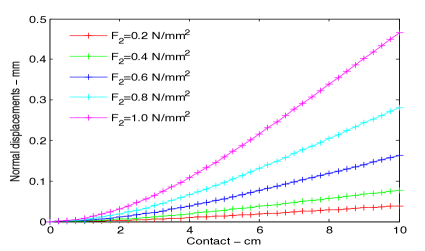
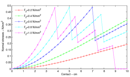
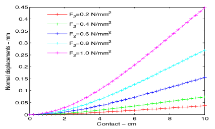
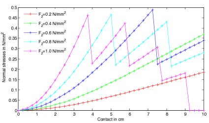
Figure 4. Upper: regularization method of [31, 33]. Lower: optimization method. Left image shows vertical displacement $u_{2}$ for 5 different values of $F_{2}$. Right image shows vertical component of reactive force along contact boundary for same 5 scenarios.

Table 1. Regularization. Vertical displacement [mm] at 4 intermediate points for same 5 scenarios.

$F_{2}[N/mm^{2}]$	$u_{2}(x_{1})$	$u_{2}(x_{2})$	$u_{2}(x_{3})$	$u_{2}(x_{4})$
0.2	4.154500e-06	1.394500e-05	2.601700e-05	3.858700e-05
0.4	8.308100e-06	2.788800e-05	5.202800e-05	7.716600e-05
0.6	1.633200e-05	5.622700e-05	1.080000e-04	1.640000e-04
0.8	2.792500e-05	9.663100e-05	1.860000e-04	2.810000e-04
1.0	4.600600e-05	1.590000e-04	3.080000e-04	4.660000e-04

Table 2. Optimization. Vertical displacement [mm] at four intermediate points for same 5 scenarios.

$F_{2}[N/mm^{2}]$	$u_{2}(x_{1})$	$u_{2}(x_{2})$	$u_{2}(x_{3})$	$u_{2}(x_{4})$
0.2	4.022500e-06	1.345400e-05	2.499300e-05	3.691900e-05
0.4	8.069300e-06	2.698800e-05	5.013300e-05	7.404900e-05
0.6	1.564800e-05	5.373900e-05	1.030000e-04	1.550000e-04
0.8	2.691300e-05	9.297200e-05	1.790000e-04	2.700000e-04
1.0	4.414000e-05	1.530000e-04	2.940000e-04	4.470000e-04

Table 3. Regularization. Horizontal displacement [mm] at four intermediate points for same 5 scenarios.

$F_{2}[N/mm^{2}]$	$u_{2}(x_{1})$	$u_{2}(x_{2})$	$u_{2}(x_{3})$	$u_{2}(x_{4})$
0.2	1.481900e-06	2.251300e-06	2.474400e-06	2.499500e-06
0.4	2.963600e-06	4.502200e-06	4.948300e-06	4.998500e-06
0.6	5.918500e-06	9.400600e-06	1.077100e-05	1.097500e-05
0.8	1.015200e-05	1.625600e-05	1.866400e-05	1.904000e-05
1.0	1.674400e-05	2.690100e-05	3.100500e-05	3.167000e-05

Table 4. Optimization. Horizontal displacement [mm] at four intermediate points for same 5 scenarios.

$F_{2}[N/mm^{2}]$	$u_{2}(x_{1})$	$u_{2}(x_{2})$	$u_{2}(x_{3})$	$u_{2}(x_{4})$
0.2	1.432200e-06	2.161500e-06	2.356100e-06	2.368400e-06
0.4	2.872700e-06	4.335000e-06	4.724700e-06	4.748800e-06
0.6	5.663400e-06	8.957000e-06	1.023200e-05	1.041100e-05
0.8	9.777300e-06	1.561000e-05	1.787700e-05	1.822600e-05
1.0	1.606400e-05	2.578000e-05	2.970700e-05	3.034700e-05

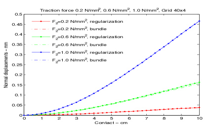
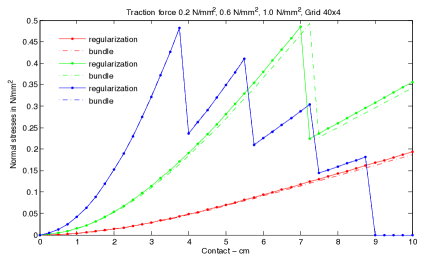
Figure 5. Comparison of regularization (bold solid curves) and optimization (dashed) for 3 different values of $F_{2}$. Left vertical displacement, right reactive force.

Table 5. Comparison of optimal valued obtained by regularization and optimization

$F_{2}[N/m^{2}]$	${\Pi_{h}}_{\rm reg}[Nm]$	${\Pi_{h}}_{\rm opt}$ [Nm]
200000	-1.32894	-1.29271
400000	-2.35224	-2.30025
600000	-3.83972	-3.74609
800000	-5.08164	-5.05389
1000000	-5.66771	-5.66770

Conclusion

We have presented a bundle method based on the mechanism of downshifted tangents which is suited to optimize upper- and lower-$C^{1}$ functions. Our method allows to integrate second-order information, if available, and gives a convergence certificate in the sense of subsequences. Every accumulation point of the sequence of serious iterates with an arbitrary starting point is critical. We have successfully applied our method to a delamination problem arising in the material sciences, where upper-$C^{1}$ functions have to be minimized. Results obtained by optimization were compared to results obtained by the regularization technique of [31, 33], and both methods are in good agreement.

References

• [1] M. Wetzel, J. Holtmannspötter, H.-J. Gudladt, J. v. Czarnecki: Sensitivity of double cantilever beam test to surface contamination and surface pretreatment. International Journal of Adhesion & Adhesives, Vol. 46, 114-121 (2013)
• [2] R. Mifflin: A modification and an extension of Lemaréchal’s algorithm for nonsmooth minimization. Math. Progr. Study 17, 77-90 (1982)
• [3] C. Lemaréchal: Bundle methods in nonsmooth optimization. In Nonsmooth optimization (Proc. IIASA Workshop, Laxenburg, 1977), pp. 79-102, IIASA Proc. Ser., 3, Pergamon, Oxford-Elmsford, N.Y., 1978.
• [4] C. Lemaréchal, C. Sagastizábal: Variable metric bundle methods: from conceptual to implementable forms. Math. Programming 76 (1997), no. 3, Ser. B, 393-410.
• [5] J. Zowe: The BT-Algorithm for minimizing a nonsmooth functional subject to linear constraints, in Nonsmooth Optimization and Related Topics , F. H. Clarke, V. F. Demyanov, F. Gianessi (eds.), Plenum Press (1989)
• [6] H. Schramm, J. Zowe: A version of the bundle idea for minimizing a nonsmooth function: conceptual idea, convergence analysis, numerical results, SIAM J. Optim. 2, 121 - 152 (1992)
• [7] D. Noll: Cutting plane oracles to minimize nonsmooth nonconvex functions. Set-Valued Var. Anal. 18 (3-4), 531-568 (2010)
• [8] D. Noll, O. Prot, A. Rondepierre: A proximity control algorithm to minimize nonsmooth nonconvex functions. Pacific J. Optim. 4 (3), 569-602 (2008)
• [9] D. Alazard, M. Gabarrou, D. Noll: Design of a flight control architecture using a nonconvex bundle method. Math. Control Sign. Syst. 25 (2), 257-290 (2013)
• [10] D. Noll: Convergence of nonsmooth descent methods using the Kurdyka-Łojasiewicz inequality. J. Optim. Theory Appl. (DOI) 10.1007/s10957-013-0391-8.
• [11] M.M. Mäkelä, M. Miettinen, L. Lukšan, J. Vlček: Comparing nonsmooth nonconvex bundle methods in solving hemivariational inequalities, Journal of Global Optimization 14 (2), 117-135 (1999).
• [12] M. Miettinen, M.M. Mäkelä, J. Haslinger: On numerical solution of hemivariational inequalities by nonsmooth optimization methods, Journal of Global Optimization 6 (4), 401-425 (1995).
• [13] L. Lukšan, J. Vlček: A Bundle-Newton method for nonsmooth unconstrained minimization, Math. Progr. 83, 373 - 391 (1998)
• [14] J. Haslinger, M. Miettinen, P.D. Panagiotopoulos: Finite Element Methods for Hemivariational Inequalities, Kluwer Academic Publishers (1999)
• [15] J. Czepiel: Proximal Bundle Method for a Simplified Unilateral Adhesion Contact Problem of Elasticity, Schedae Informaticae 20, 115-136 (2011)
• [16] L. Nesemann, E.P. Stephan: Numerical solution of an adhesion problem with FEM and BEM, Appl. Numer. Math. 62 (5), 606-619 (2012)
• [17] M. Kočvara, A. Mielke, T. Roubíček: A rate-independent approach to the delamination problem, Math. Mech. Solids 11, No. 4, 423-447 (2006)
• [18] T. Roubíček, V. Mantic, Panagiotopoulos, C.G.: A quasistatic mixed-mode delamination model, Discrete Contin. Dyn. Syst., Ser. S 6, No. 2, 591-610 (2013)
• [19] J. E. Spingarn: Submonotone subdifferentials of Lipschitz functions. Trans. Amer. Math. Soc. 264, 77-89 (1981)
• [20] A. Daniilidis, P. Georgiev: Approximate convexity and submonotonicity. J. Math. Anal. Appl. 291, 117-144 (2004)
• [21] R. T. Rockafellar, R. J-B. Wets: Variational Analysis. Springer Verlag (2004)
• [22] A. Daniilidis, J. Malick: Filling the gap between lower-$C^{1}$ and lower-$C^{2}$ functions. Journal of Convex Analysis 12(2), 2005, pp. 315 – 329.
• [23] R. A. Poliquin, R. T. Rockafellar: Prox-regular functions in variational analysis, Trans. Amer. Math. Soc. 348 (5), 1805 - 1838 (1996)
• [24] K.C. Kiwiel: An aggregate subgradient method for nonsmooth convex minimization, Math. Programming 27, 320 - 341 (1983)
• [25] J. Cullum, W.E. Donath, P. Wolfe: The minimization of certain nondifferential sums of eigenvalues of symmetric matrices. Math. Progr. Stud. 3, 35-55 (1975)
• [26] P. Apkarian, D. Noll, O. Prot: A trust region spectral bundle method for nonconvex eigenvalue optimization, SIAM J. Optim. 10 (1), 281-306 (2008)
• [27] A. Ruszczyński: Nonlinear optimization, Princeton University Press (2006)
• [28] J.-B. Hiriart-Urruty, C. Lemaréchal: Convex Analysis and Minimization Algorithms, vol. I and II: Advanced Theory and Bundle Methods, vol. 306 of Grundlehren der mathematischen Wissenschaften, Springer Verlag, New York, Heidelberg, Berlin (1993)
• [29] W. L. Hare, C. Sagastizabal: Computing proximal points of nonconvex functions, Math. Programming series B 116, 221-258 (2009)
• [30] Z. Naniewicz, P.D. Panagiotopoulos: Mathematical Theory of Hemivariational Inequalities and Applications, New York (1995).
• [31] N. Ovcharova: Regularization Methods and Finite Element Approximation of Hemivariational Inequalities with Applications to Nonmonotone Contact Problems, PhD Thesis, Universität der Bundeswehr München, Cuvillier Verlag, Göttingen (2012).
• [32] N. Ovcharova, J. Gwinner: A study of regularization techniques of nondifferentiable optimization in view of application to hemivariational inequalities, accepted for publication in JOTA, JOTA-D-13-00163
• [33] Ovcharova, N., Gwinner. J: On the regularization method in nondifferentiable optimization applied to hemivariational inequalities, Constructive Nonsmooth Analysis and Related Topics, Springer, 59-70 (2013).
• [34] C.C. Baniotopoulos, J. Haslinger, Z. Morávková: Contact problems with nonmonotone friction: discretization and numerical realization, Comput. Mech. 40, 157-165 (2007)
• [35] C.C. Baniotopoulos, J. Haslinger, Z. Morávková: Mathematical modeling of delamination and nonmonotone friction problems by hemivariational inequalities, Applications of Mathematics 50 (1), 1-25 (2005)
• [36] S. Carl, V.K. Le, D. Motreanu: Nonsmooth Variational Problems and Their Inequalities, Springer (2007)
• [37] R. Glowinski: Numerical Methods for Nonlinear Variational Problems, Springer, New York (1984)
• [38] D. Goeleven, D. Motreanu, Y. Dumont, M. Rochdi, M.: Variational and Hemivariational Inequalities: Theory, Methods and Applications, Vol. I: Unilateral Analysis and Unilateral Mechanics, Vol. II: Unilateral problems, Kluwer (2003)
• [39] J. Gwinner: Finite-element convergence for contact problems in plane linear elastostatics, Quarterly of Applied Mathematics, Vol. 50, 11-25 (1992)
• [40] J. Gwinner: hp-FEM convergence for unilateral contact problems with Tresca friction in plane linear elastostatics, J. Comput. Appl. Math., Vol. 254, 175-184 (2013)
• [41] P.D. Panagiotopoulos: Hemivariational inequalities. Applications in mechanics and engineering, Berlin, Springer (1993)
• [42] P.D. Panagiotopoulos: Inequality problems in mechanics and application. Convex and nonconvex energy functions, Basel, Birkhäuser (1998)
• [43] M. Sofonea, A. Matei: Variational Inequalities with Applications, Springer (2009)