Slotted Aloha for Networked Base Stations

Abstract

We study multiple base station, multi-access systems in which the user-base station adjacency is induced by geographical proximity. At each slot, each user transmits (is active) with a certain probability, independently of other users, and is heard by all base stations within the distance $r$. Both the users and base stations are placed uniformly at random over the (unit) area. We first consider a non-cooperative decoding where base stations work in isolation, but a user is decoded as soon as one of its nearby base stations reads a clean signal from it. We find the decoding probability and quantify the gains introduced by multiple base stations. Specifically, the peak throughput increases linearly with the number of base stations $m$ and is roughly $m/4$ larger than the throughput of a single-base station that uses standard slotted Aloha. Next, we propose a cooperative decoding, where the mutually close base stations inform each other whenever they decode a user inside their coverage overlap. At each base station, the messages received from the nearby stations help resolve collisions by the interference cancellation mechanism. Building from our exact formulas for the non-cooperative case, we provide a heuristic formula for the cooperative decoding probability that reflects well the actual performance. Finally, we demonstrate by simulation significant gains of cooperation with respect to the non-cooperative decoding.

I Introduction

Slotted Aloha [1] and framed slotted Aloha [2] are well-known schemes for uncoordinated multiple access that date back to the 70s. With these schemes, the time is divided into slots, and, at each slot, users contend to transmit their packets to the base station. With slotted Aloha, each user transmits at each slot with a certain probability; with framed slotted Aloha, slots are grouped into frames, and each user randomly selects a slot at each frame to transmit.

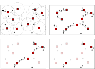
Figure 1: Top left: Illustration of the multi-access system. Red squares represent base stations. Full circles represent active users, while empty circles represent inactive users. Top right, bottom left, and bottom right depict, respectively, first, second, and third iteration of the cooperative decoding algorithm for the network example in the top left figure. An edge is labeled with one at iteration $t$ if its incident user gets collected at $t$; such an edge is erased at $t+1$; an edge is labeled with $0$ at iteration $t$ if its incident user is unknown (not decoded) up to and at iteration $t$.

In the past decade, there has been much progress in the development of slotted Aloha type protocols, e.g., [3, 4, 5], with dramatic throughput improvements. Reference [3] introduces a framed protocol that allows for multiple user transmissions, as considered in [6] in the past, but with a novel successive interference cancelation mechanism [3]. In [3], users transmit (are active) at multiple slots at each frame, and send, along with their packet replicas, pointers to the corresponding activation slots. When a slot with a single active user occurs, this allows the base station not only collect this user, but also subtract its contribution in each other slot the user was active. This likely resolves collisions in some of the past slots and thereby allows for collecting additional users. More recently, [4] demonstrates that successive interference cancelation is analogous to the belief propagation erasure-decoding of the codes on graphs. Exploiting this analogy, [4] introduces a variable number of users’ transmission attempts and optimizes their distribution to maximize the throughput. Building on an analogy with rateless codes, reference [5] introduces the frameless Aloha protocol that further enhances the throughput. With the protocol therein, the frame size is not fixed a priori, but rather it adds new slots until a desired fraction of decoded users is achieved.

All the above references exploit temporal diversity. Reference [7] considers multiple receiver multi-access systems with spatial diversity which arises from independent fading of different user-receiver links. It analyzes the capture performance of the system under Rayleigh fading and shadowing. A recent reference [8] also considers a multiple receiver case with spatial diversity. Under independent on-off fading, it quantifies analytically the gains in the throughput introduced by multiple receivers (over the single receiver case), as well as the impact of the fading probability on these gains.

In this paper, we also study the spatial diversity effects with multiple receivers, but under a very different model than the ones in [7, 8]. A total of $m$ base stations (receivers) are deployed over a (unit) geographic area, and they jointly serve $n$ users (transmitters). Both the users and base stations are placed uniformly at random over the area. At a fixed time slot, each user transmits (is active) with probability $p$, independently from other users. Each base station can hear all active users that are within distance $r$ from it, where $r$ is small compared to the diameter of the area. The base station thus receives a superposition of the signals of active users in its $r$-neighborhood. (The signals of the users outside the $r$-neighborhood do not contribute to the signal.)

We first consider the slotted Aloha protocol where each base station performs decoding in isolation (without cooperating with other stations). It decodes a user whenever there is a single active user in its $r$-neighborhood. We find the probability that an arbitrary fixed user is decoded, both in the finite regime and asymptotically, when $n,m\rightarrow\infty$ and $r\rightarrow 0$ ($p$-fixed.) Further, we quantify the gains of diversity introduced with multiple base stations. In particular, the peak throughput (expected number of decoded users per slot) is increased $\delta\,m$ times with respect to the single-base station slotted Aloha, where $\delta$ is a positive constant. (In particular, $\delta\approx 1/4$, see Section IV for details.) In other words, the throughput scales linearly with $m$. For example, for $m=100$ and $r\approx 0.1$, the peak throughput is about $20$.

Next, we propose a cooperative, iterative decoding where the base stations that are geographically close communicate during decoding iterations. Specifically, we assume that, if a base station detects a user, it knows at which other base stations this user is also heard, and it informs them of this users’ ID and its information packet. The contacted base stations can subtract the interference contribution of the received signal, which possibly reveals additional clean packet readings. We show by simulation that cooperation introduces significant gains in the system performance. For example, for $m=100$ and $r\approx 0.1$, the peak throughput increases from $20$ (no cooperation) to $33$ (with cooperation). Also, the maximal load for which the decoding probability is above a prescribed value (e.g., $0.95$) is about $3$ times larger under cooperation than without cooperation, for a wide range of $r$.

Structurally, this decoding algorithm is analogous to the interference cancellation decoding in, e.g., [4, 3], and it can be represented via message passing on a bipartite graph like in [4]. Active users here correspond to users in [4], base stations correspond to different slots (check nodes) in [4], and the links are the physical links between active users and base stations. However, the structure of the graph here is induced by geometry and is very different from the random graph in [4]. (See Section III for details.) Evaluating the decoding probability here is very challenging and standard tools like and-or-tree analysis [9] do not directly apply. We make the first step towards this goal by giving a heuristic formula that reflects well the actual performance. We derive the heuristic building from our results for the non-cooperative decoding.

In this paper, cooperation among base stations is confined within a single time slot and is independent across slots. In other words, this paper exploits spatial diversity. In our ongoing work, we exploit the potential of both spatial and temporal diversity by allowing that base stations cooperate both across space (as considered here) and across slots. The motivation for this comes from the single base station systems, where successive interference cancellation across slots yields dramatic throughput improvements.

Finally, we believe that our studies have a potential to find applications in massive uncoordinated multiple access in various networks, such as cellular, satellite, and vehicular networks, including recently popular machine-to-machine (M2M) services over these networks.

Paper organization. The next paragraph introduces notation. Section II details the system model that we assume, and Section III presents our decoding algorithms. Section IV presents our results on the performance of the two decoding algorithms. Section V gives numerical studies and interpretations. Finally, we conclude in Section VI.

Notation. We denote by: $\mathbf{B}(q,s)$ the Euclidean ball in the $2$-dimensional space centered at $q$ with radius $s$; $\mathbf{B}_{\infty}(q,s)$ the square centered at $q$, with the side length equal to $2s$; $1_{E}$ the indicator of event $E$; $\mathbb{P}$ and $\mathbb{E}$ the probability and expectation operators, respectively.

II System model

We consider a multi-access system with $n$ users and $m$ base stations. We denote by $U_{i}$, $i=1,...,n$ a user, and by $B_{l}$, $l=1,...,m$, a base station. Users and base stations are distributed over a geographical area, and each user $U_{i}$ can be heard by all base stations within distance $r$ from $U_{i}$. (See Figure 1, top left, for an illustration.) The time is divided into slots. As the number of users $n$ may be larger than the number of base stations $m$ (as is common in practical scenarios), to avoid excessive collisions, different users’ transmissions are distributed across time slots, i.e., only a subset of users transmits at a certain slot. In this paper, we assume that decoding is completely decoupled (independent) across slots. Henceforth, from now on, it suffices to consider the system at a single, fixed slot. To keep the exposition general, we assume that each user $U_{i}$ transmits its message at a fixed slot with probability $p$, independently from other users, and that all transmissions are slot-synchronized. This model subsumes, e.g., the following system. There are $\tau$ available slots in each frame. Users’ and base stations’ placements are fixed during the frame. Each user transmits once per frame, with equal probability across the $\tau$ slots. In our model, this corresponds to setting $p=1/\tau$. We say that a user is active at a certain slot if it transmits at this slot.

We let $G:=np/m$, and we call $G$ the normalized load. The quantity $G$ equals the expected number of active users at a fixed slot per base station. The message of user $U_{i}$ contains the information packet and a header with the user’s ID. If $U_{i}$ is within distance $r$ from $B_{l}$, we say that $U_{i}$ and $B_{l}$ are adjacent. Each base station $B_{l}$ therefore hears a superposition (collided message in general) $y_{l}$ from all active adjacent users. We explain decoding mechanism in Section III.

We now detail the placement model at a fixed slot. Both users and base stations at a fixed slot are placed in the unit square $\mathcal{A}=\mathbf{B}_{\infty}(0,1/2)$, centered at $(0,0)$. User $U_{i}$ is situated at a location $u_{i}$, where $u_{i}$ is selected from $\mathcal{A}$ uniformly at random, independently from other user’s locations. Further, base station $B_{l}$ is positioned at a location $b_{l}$, where $b_{l}$ is selected from $\mathcal{A}$ uniformly at random, independently from other stations’ locations. We assume that the placements of users and base stations are also mutually independent.

For the purpose of analysis, we differ two types of placements. We define $\mathcal{A}^{\mathrm{o},r}:=\mathbf{B}_{\infty}(0,1/2-2r)$, and say that a user is nominally placed if its position is in $\mathcal{A}^{\mathrm{o},r}$, and similarly for a base station. If, on the other hand, a user or a base station lies in the strip $\partial\mathcal{A}^{r}$ along the boundary of $\mathcal{A}$, $\partial\mathcal{A}^{r}:=\mathcal{A}\setminus\mathcal{A}^{\mathrm{o},r}$, we call this a boundary placement. Since placements are uniform over $\mathcal{A}$, the probability of the nominal placement is $(1-4r)^{2}$, and the probability of the boundary placement is $1-(1-4r)^{2}=8r-16r^{2}$. We see that, as the radius $r$ decreases, the probability of the nominal placement goes to one, and hence we can neglect in the analysis all the effects caused by the boundary placements.

Degree distributions. For future reference, we introduce the users’ and base stations’ degree distributions when they are nominally placed. Fix arbitrary user $U_{i}$, and arbitrary point $q\in\mathcal{A}^{\mathrm{o},r}$, and let $\Lambda_{d}=\mathbb{P}\left(\mathrm{deg}(U_{i})=d\,|\,u_{i}=q\right)$, i.e., $\Lambda_{d}$ is the conditional probability that $U_{i}$ has exactly $d$ adjacent base stations, given that it is nominally placed. It is easy to show that degrees follow binomial distribution, i.e., $\Lambda_{d}={m\choose d}(r^{2}\pi)^{d}(1-r^{2}\pi)^{m-d},$ $d=0,...,m$. Similarly, let $\Psi_{d}=\mathbb{P}\left(\mathrm{deg}(B_{l})=d\,|\,b_{l}=q\right)$, where $\mathrm{deg}(B_{l})$ denotes the number of active users $U_{j}$, $j\in\{1,...,n\}\setminus\{i\}$, adjacent to $B_{l}$. (We exclude arbitrary fixed user $U_{i}$, as needed for subsequent analysis.) We have $\Psi_{d}={n-1\choose d}(p\,r^{2}\pi)^{d}(1-p\,r^{2}\pi)^{n-1-d}$, $d=0,...,n-1$. We will also be interested in the asymptotic regime, when $n\rightarrow\infty$, $r=r(n)\rightarrow 0$, and $m=m(n)\rightarrow\infty$ ($p$ is fixed), such that $mr^{2}\pi\rightarrow\lambda,$ $np\,r^{2}\pi\rightarrow\psi,$ where $\lambda,\psi>0$ are constants. In such setting, the users’ and base stations’ degree distributions converge to Poisson distributions with parameters $\lambda$ and $\psi$, respectively, i.e., for all $d=0,1,...$:

$$\Lambda_{d}\rightarrow\Lambda_{\infty,d}:=e^{-\lambda}\frac{\lambda^{d}}{d!},\>\>\>\>\Psi_{d}\rightarrow\Psi_{\infty,d}:=e^{-\psi}\frac{\psi^{d}}{d!}.$$ (1)

Hence, in the asymptotic regime, $\lambda$ is the average number of base stations adjacent to a fixed user $U_{i}$, and $\psi$ is the average number of active users adjacent to a fixed base station $B_{l}$. It is easy to see that $\lambda$ and $\psi$ are related as $\psi=G\,\lambda$.

Coverage. Consider $\mathbb{E}\left[\frac{1}{n}\sum_{i=1}^{n}1_{\left\{U_{i}\mathrm{\;cov.}\right\}}\right]=\mathbb{P}\left(U_{i}\mathrm{\;cov.}\right)$, where the event $\left\{U_{i}\mathrm{\;cov.}\right\}$ means that $U_{i}$ is heard (“covered”) by at least one base station. We refer to the latter quantity as the expected coverage. We have $P\left(U_{i}\mathrm{\;cov.}\,|\,u_{i}\in\mathcal{A}^{\mathrm{o},r}\right)=1-\Lambda_{0}$, and $\mathbb{P}\left(U_{i}\mathrm{\;cov.}\right)\rightarrow 1-\Lambda_{\infty,0}=1-\mathrm{exp}(-\lambda)$. An active user $U_{i}$ can be collected only if it is covered, no matter what decoding is used. Therefore, for a high decoding probability, we cannot have $\lambda$ (or $r$) too small. Henceforth, from now on we assume $\lambda\geq\lambda_{\mathrm{min}}(\epsilon):=\mathrm{ln}(1/\epsilon)$, such that $1-\epsilon$ coverage is ensured; e.g., for $\epsilon=0.05$, $\lambda_{\mathrm{min}}(\epsilon)\approx 3$.

III Decoding algorithms

Subsection III-A details the non-cooperative decoding, and Subsection III-B details the cooperative decoding algorithm.

III-A Non-cooperative decoding

We now explain the non-cooperative decoding algorithm, where each base station works in isolation. At each base station, decoding is the simple slotted Aloha decoding. Suppose that station $B_{l}$ received signal $y_{l}$. We assume that $B_{l}$ can determine if $y_{l}$ corresponds to a “clean” message. In other words, if, at a fixed slot, there is a single active user $U_{i}$ in $\mathbf{B}(b_{l},r)$ then $B_{l}$ collects user $U_{i}$ (it reads its packet and obtains its ID). We say that a user is collected at a fixed time slot if it is collected by at least one base station at this slot. For example, for the network in Figure 1, top left, we can see that $4$ out of $10$ active users are collected.

III-B Cooperative decoding

We now present the cooperative decoding algorithm, where neighboring base station collaborate to collect users. We assume that each base station $B_{l}$ is aware of which users (either active or inactive) it covers, i.e., it knows the IDs of all its adjacent users (e.g., through some sort of association procedure). Further, for each of its adjacent users $U_{i}$, $B_{l}$ knows the list of the base stations $B_{k}$, $k\neq l$, to which $U_{i}$ is also adjacent. We say that two base stations are neighbors if they share at least one user. The decoding is iterative and involves communication between neighboring base stations. Each base station $B_{l}$ maintains over iterations $t$, $t=0,1,...,$ a signal $z_{l}=z_{l}(t)$. Initially, at $t=0$, $z_{l}(t)$ is the received signal $y_{l}$ from its active adjacent users (either a clean message from an active user, a collided message, or an empty message if neither of the users in $\mathbf{B}(b_{l},r)$ is active.) Station $B_{l}$ at a certain iteration $t$ may receive a message $x^{(k)}$ from a neighboring base station $B_{k}$. This happens if $B_{k}$ decodes a user at $t$, which we call $U^{(k)}$, and if $U^{(k)}$ is adjacent to both $B_{l}$ and $B_{k}$. The message $x^{(k)}$ contains the packet of user $U^{(k)}$ and its ID. Upon reception of $x^{(k)}$, station $B_{l}$ subtracts the interference contribution of user $U^{(k)}$, which we symbolically write as $z_{l}\leftarrow z_{l}-x^{(k)}$. Station $B_{l}$ can recognize if the updated signal $z_{l}$ corresponds to a clean packet, and, if so, it reads the packet and determines to which user it belongs. The decoding algorithm operates as follows. At iteration $t$, $t=1,2,...$, all base stations work in synchrony and perform the same steps. Iteration $t$ at an arbitrary station $B_{l}$ has three steps: 1) check signal, 2) collect and transmit, and 3) receive and update. The last two steps always occur exclusively, i.e., one and only one among the two is always performed. As we will see, each base station performs at most $m$ iterations. We assume that all stations know $m$ beforehand.

Step 1: Check signal: $B_{l}$ checks whether signal $z_{l}$ corresponds to a “clean” packet. If this is true, it performs the collect and transmit step; otherwise, it performs the receive and update step.

Step 2: Collect and transmit: $B_{l}$ collects a user $U^{(l)}$ and reads its ID. It transmits message $x^{(l)}$ to all $B_{k}$’s, $k\neq l$, that are adjacent to $U^{(l)}$. We call the latter set of stations $\Omega^{(l)}.$ After transmissions, $B_{l}$ leaves the algorithm.

Step 3: Receive and update: $B_{l}$ scans over all messages $x^{(k)}$ that it received at $t$ and identifies the subset $\mathcal{J}^{(l)}$ of all distinct messages. Subsequently, $B_{l}$ subtracts from $z_{l}$ the interference contributions from all $x_{j}$’s, $j\in\mathcal{J}^{(l)}$, which we symbolically write as $z_{l}\leftarrow z_{l}-\sum_{j\in\mathcal{J}^{(l)}}x_{j}$. Set $t\leftarrow t+1$. If $t=m$, $B_{l}$ leaves the algorithm; otherwise, it goes to step 1.

Graph representation of decoding. We now introduce a graphical message-passing representation of decoding. It involves the evolution of a bipartite graph $\mathcal{G}_{t}$ over iterations $t$. Graph $\mathcal{G}_{t}$ has two types of nodes – base stations and active users. Both the node sets and the edge set change (reduce) over iterations $t$. It is initialized by $\mathcal{G}_{0}$, where $\mathcal{G}_{0}$ is defined as follows: it has the node set that consists of all base stations and all active users. Its set of links contains all pairs $(B_{l},U_{i})$ such that $B_{l}$ and $U_{i}$ are within distance $r$ from each other (and $U_{i}$ is active.) We now describe one iteration $t$.

Graph decoding iteration. All $B_{l}$’s in $\mathcal{G}_{t}$ check in parallel if their degree in $\mathcal{G}_{t}$ equals one. Let $\mathcal{L}_{t}\subset\{1,...,m\}$ be the set of degree one base stations in $\mathcal{G}_{t}$. If $\mathcal{L}_{t}$ is empty, the algorithm terminates. Otherwise, for each $l\in\mathcal{L}_{t}$, let $U^{(l)}$ be the user adjacent to $B_{l}$. Remove from $\mathcal{G}_{t}$ all $B_{l}$’s and $U^{(l)}$’s, $l\in\mathcal{L}_{t}$, and all the links incident to $U^{(l)}$, $l\in\mathcal{L}_{t}$. Set $t\leftarrow t+1$.

It is easy to see that the above algorithm terminates after at most $m$ iterations. Namely, at each iteration $t$, either at least one base station node is removed, or the algorithm terminates at $t$. Therefore, at most $m$ iterations can be performed. For the network in Figure 1, top left, we show decoding iterations in Figures 1, top right (at $t=1$), bottom left ($t=2$), and bottom right ($t=3$). We can see that cooperative decoding collects $9$ out of $10$ users, while the non-cooperative collected $4$.

IV Performance analysis

In this section, we study the performance of both non-cooperative and cooperative decoding schemes. Specifically, our goal is to determine the expected fraction of decoded users per time slot, $\mathbb{E}\left[\frac{1}{n}\sum_{i=1}^{n}1_{\left\{U_{i}\mathrm{\;coll.}\right\}}\right].$ Exploiting the symmetry across users, we have that the above quantity equals $(1/n)\,n\,\mathbb{P}\left(U_{i}\mathrm{\;coll.}\right)$ = $\mathbb{P}\left(U_{i}\mathrm{\;coll.}\right).$ Hence, our task reduces to finding the probability that arbitrary fixed user $U_{i}$ is collected. The following simple relation will be useful throughout: $\mathbb{P}\left(U_{i}\mathrm{\;coll.}\right)=p\,\mathbb{P}\left(U_{i}\mathrm{\;coll.}\,|\,U_{i}\mathrm{\;act.}\right)$, which is easily obtained after conditioning on the event that $U_{i}$ is active and using that $p$ is the probability of $U_{i}$ being active. (Here, abbreviation “$U_{i}$ coll.” stands for $U_{i}$ is collected, and “$U_{i}$ act.” stands for $U_{i}$ is active.) We also consider the normalized, per station throughput $T(G)=(1/m)\mathbb{E}\left[\sum_{i=1}^{n}1_{\left\{U_{i}\mathrm{\;coll.}\right\}}\right]$ – the expected total number of collected users per slot, per station. Next, recall $\lambda=mr^{2}\pi$, and, for fixed $m,p,$ and $r$, we will be interested in the following quantity:

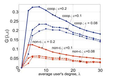
Figure 2: Simulated quantity ${G^{\bullet}(\lambda,\epsilon)}$ in (2) versus the average user’s degree $\lambda=mr^{2}\pi$ for different values of $\epsilon\in\{0.08;0.1;0.2\}$.

$${G^{\bullet}(\lambda,\epsilon)}=\sup\left\{G\geq 0:\,\,\mathbb{P}\left(U_{i}\mathrm{\;coll.}\,|\,U_{i}\mathrm{\;act.}\right)\geq 1-\epsilon\right\},$$ (2)

where $\epsilon>0$ is a small number. In words, ${G^{\bullet}(\lambda,\epsilon)}$ is the largest normalized load for which decoding probability $\mathbb{P}\left(U_{i}\mathrm{\;coll.}\,|\,U_{i}\mathrm{\;act.}\right)$ is above the prescribed value $1-\epsilon$. Recall $P\left(U_{i}\,\,\mathrm{cov.}\right)$ and that $P\left(U_{i}\,\,\mathrm{cov.}\right)\approx 1-\Lambda_{0}$. It is clear that, when $1-\epsilon>P\left(U_{i}\,\,\mathrm{cov.}\right)$, due to the relation $\mathbb{P}\left(U_{i}\mathrm{\;coll.}\,|\,U_{i}\mathrm{\;act.}\right)\leq P\left(U_{i}\,\,\mathrm{cov.}\right)$, $\mathbb{P}\left(U_{i}\mathrm{\;coll.}\,|\,U_{i}\mathrm{\;act.}\right)$ cannot be greater or equal $1-\epsilon$ for any $G$, i.e., no matter how small $G$ is. Thus, whenever $1-\epsilon>P\left(U_{i}\,\,\mathrm{cov.}\right)$, by convention we say ${G^{\bullet}(\lambda,\epsilon)}=0.$

Remark 1

We explain the motivation behind quantity ${G^{\bullet}(\lambda,\epsilon)}$. Suppose there are $\tau$ available slots, where each user is active in exactly one among the slots. The system has the following requirement on the “quality of service” – each user $U_{i}$ be collected with probability above $1-\epsilon$. This translates into the requirement $\mathbb{P}\left(U_{i}\mathrm{\;coll.}\,|\,U_{i}\mathrm{\;act.}\right)\geq 1-\epsilon.$ For a fixed $m,p,r$, we ask what is the maximal number of users that can be served with the guaranteed quality of service. That is, we look for $\sup\{n:\,\mathbb{P}\left(U_{i}\mathrm{\;coll.}\,|\,U_{i}\mathrm{\;act.}\right)\geq 1-\epsilon\}$. As $m,p,r$, are fixed and $G=np/m$, this is equivalent to finding (2). We will later be interested in optimizing (maximizing) ${G^{\bullet}(\lambda,\epsilon)}$.

IV-A Non-cooperative decoding

We now characterize $\mathbb{P}\left(U_{i}\mathrm{\;coll.}\right)$ for the non-cooperative decoding. As we will see, the sought probability depends on the distributions of the areas covered by randomly generated balls. Specifically, consider the ball $\mathbf{B}(0,r)$. Fix some $k\geq 1$, and generate randomly $k$ points $q_{1},...,q_{k}$, where $q_{l}$’s, $l=1,...,k$, are drawn mutually independently from the uniform distribution on $\mathbf{B}(0,r)$, and let $\alpha_{k}$ be the random variable that equals the area of $\cup_{l=1,...,k}\mathbf{B}(q_{l},r)$ divided (normalized) by $r^{2}\pi$. Further, denote by $\mu_{k}$ the probability distribution on $[0,\infty)$ induced by $\alpha_{k}$. Clearly, $\alpha_{k}$ (and hence $\mu_{k}$) does not depend on $r$ due to normalization. Hence, we can set $r=1$. Also, it is easy to see that $\alpha_{1}=1$ with probability one, i.e., $\mu_{1}$ is the Dirac distribution at $1$. Also, for any $k$, $1\leq\alpha_{k}\leq 4$, with probability one, i.e., $\mu_{k}$ is supported on $[1,4]$. This is because all the $q_{l}$’s, $l=1,...,k$, belong to $\mathbf{B}(0,1)$, and thus $\cup_{l=1,...,k}\mathbf{B}(q_{l},1)$ is always a subset of $\mathbf{B}(0,2)$. The distributions $\mu_{k}$, $k=2,...,m$, are difficult to compute. However, they can be partially characterized by estimating the first $s_{\mathrm{max}}$ moments $\overline{\alpha}_{k}^{(s)}:=\int_{1}^{4}a^{s}\,d\mu_{k}(a)$, $s=1,...,s_{\mathrm{max}}$. This can be done, e.g., through Monte Carlo simulations. We emphasize that the moments $\overline{\alpha}_{k}^{(s)}$, $s=1,...,s_{\mathrm{max}}$, $k=2,...,m$, need to be tabulated only once (just like, e.g., the tail distribution of the standard Gaussian.) That is, once we have the $\overline{\alpha}_{k}^{(s)}$’s available, they apply for any set of parameters $n,m,p,r$.

We now state our result on $\mathbb{P}\left(U_{i}\mathrm{\;coll.}\,|\,U_{i}\mathrm{\;act.}\right)$ and $T(G)$. We distinguish two cases: 1) non-asymptotic regime of finite $r,n,m$, that corresponds to (binomial) degree distributions $\Lambda_{d},\Psi_{d}$; and 2) asymptotic regime that corresponds to (Poisson) degree distributions $\Lambda_{\infty,d}$, $\Psi_{\infty,d}$.

Theorem 1

Consider the non-cooperative decoding algorithm. Then, for $r\leq 1/4$, we have: $p\,P_{\mathrm{coll.}}^{\,\mathrm{o},r}\leq\mathbb{P}\left(U_{i}\mathrm{\;coll.}\right)\leq p\,\left(P_{\mathrm{coll.}}^{\,\mathrm{o},r}+8r-16r^{2}\right),$ where $P_{\,\mathrm{coll.}}^{\mathrm{o},r}=\mathbb{P}\left(U_{i}\mathrm{\;coll.}\,|\,U_{i}\mathrm{\;act.},\,u_{i}\in\mathcal{A}^{\mathrm{o},r}\right)$ and equals:

$$P_{\,\mathrm{coll.}}^{\mathrm{o},r}=\sum_{k=1}^{m}(-1)^{k-1}\,\zeta_{k}\,{I_{k}},\;\;\;\zeta_{k}=\sum_{d=k}^{m}{d\choose k}\,\Lambda_{d},$$ (3)

and ${I_{k}}=\int_{a=1}^{4}\left(1-p\,r^{2}\pi a\right)^{n-1}\,d\mu_{k}(a).$ Further, let $p$ be fixed, $n\rightarrow\infty$, $m=m(n)\rightarrow\infty$, and $r=r(n)\rightarrow 0$, and recall $\lambda,\psi$ in (1). Then, $\mathbb{P}\left(U_{i}\mathrm{\;coll.}\right)\rightarrow p\,\sum_{k=1}^{\infty}(-1)^{k-1}\,\frac{\lambda^{k}}{k!}\,{I_{\infty,k}},$ where ${I_{\infty,k}}=\int_{a=1}^{4}e^{-\psi\,a}\,d\mu_{k}(a).$

We briefly comment on the structure of the results. It can be seen that $\zeta_{k}\rightarrow\lambda^{k}/k!$. This is because $\Lambda_{d}\rightarrow\Lambda_{\infty,d}$ in (1), and so $\zeta_{k}\rightarrow\sum_{d=k}^{\infty}{d\choose k}e^{-\lambda}\lambda^{d}/d!=\sum_{d=k}^{\infty}\frac{d!}{(d-k)!\,k!}\,e^{-\lambda}\frac{\lambda^{d}}{d!}=\lambda^{k}/k!$. Similarly, it can be shown that ${I_{k}}\rightarrow{I_{\infty,k}}$.

Sketch of the proof. The detailed technical proof of Theorem 1 is omitted due to lack of space and will be provided in a companion journal paper. We briefly sketch the proof of (3), highlighting the main steps and omitting certain arguments. The keys are to use the inclusion-exclusion principle, conditioning on a user’s degree, and considering the size of the areas covered by the user’s neighboring base stations. We consider a user $U_{i}$ at the fixed nominal placement $u_{i}=q$, $q\in\mathcal{A}^{\mathrm{o},r}$. Consider $\mathbb{P}\left(U_{i}\mathrm{\;coll.}\,|\,U_{i}\mathrm{\;act.},\,u_{i}=q\right)$. We first use the total probability law with respect to the degree $\mathrm{deg}(U_{i})$:

$$\mathbb{P}\left(U_{i}\mathrm{\;coll.}\,|\,U_{i}\mathrm{\;act.},\,u_{i}=q\right)=\sum_{d=1}^{m}\gamma(d)\,\Lambda_{d},$$ (4)

where $\gamma(d)=\mathbb{P}\left(U_{i}\mathrm{\,coll.}\,|\,U_{i}\mathrm{\,act.,}\,U_{i}=q\,\,\mathrm{deg}(U_{i})=d\right)$. Due to base stations’ symmetry, without loss of generality we can assume that $B_{1},...,B_{d}$ are the neighbors. In other words, $\gamma(d)$ actually equals the probability that $U_{i}$ is collected, given that $U_{i}$ is active, $U_{i}$ is nominally placed at $q$, and $B_{1},...,B_{d}$ are its neighbors. Now, $U_{i}$ is collected if and only if at least one of the $B_{l}$’s decodes it, and $B_{l}$ collects $U_{i}$ if and only if $U_{i}$ is the only active user in $\mathbf{B}(b_{l},r)$. (We then say that $B_{l}$ is empty.) Summarizing, $\gamma(d)$ is the conditional probability of the union $\cup_{l=1}^{d}\{B_{l}\mathrm{\,\mathrm{empty}}\}$, given that the $U_{i}$’s neighbors are $B_{1},...,B_{d}$, $u_{i}=q$, $U_{i}$-active. Now, applying the inclusion-exclusion formula:

$$\gamma(d)=\sum_{k=1}^{d}(-1)^{k-1}{d\choose k}\eta(k,d),$$ (5)

where $\eta(k,d)$ is the conditional probability of $\cap_{l=1}^{k}\{B_{l}\mathrm{\;empty}\}$, conditioned on $B_{1},...,B_{d}$ be neighbors, $u_{i}=q$, $U_{i}$-active. Intuitively, $\eta(k,d)$ depends on the area of $\cup_{l=1}^{k}\mathbf{B}(b_{l},r)$, because we look at the event that no active users lie in $\cup_{l=1}^{k}\mathbf{B}(b_{l},r)$. It can be shown (proof omitted) that $\eta(k):=\eta(k,d)$ equals $I_{k}$ in Theorem 1 and is independent of $d$. Substituting $\eta(k,d)=I_{k}$ in (5), plugging the resulting equation in (4), and noting that the probability in (4) is the same for all nominal $q$’s, we obtain (3).

Numerical calculation. Theorem 1 expresses $P\left(U_{i}\mathrm{\;coll.}\right)$ in the form that is difficult to compute. Assuming that the first moments $\overline{\alpha}_{k}:=\overline{\alpha}_{k}^{(1)}$, $k=1,...,k_{\mathrm{max}}$ are available (e.g., obtained through Monte Carlo simulations), we can compute $\mathbb{P}\left(U_{i}\mathrm{\;coll.}\right)$ with a high accuracy and a small computational cost, through the formula:

$$\mathbb{P}\left(U_{i}\mathrm{\;coll.}\right)\approx p\,\sum_{k=1}^{k_{\mathrm{max}}}(-1)^{k-1}\,\frac{\lambda^{k}}{k!}\,e^{-\overline{\alpha}_{k}\,\psi}.$$ (6)

Here, we approximated $\sum_{k=1}^{\infty}(-1)^{k-1}\lambda^{k}/k!I_{\infty,k}$ at $k=k_{\mathrm{max}}$ by letting ${I_{\infty,k}}\approx e^{-\overline{\alpha}_{k}\,\psi}$ and truncating the infinite sum at $k=k_{\mathrm{max}}$. Formula (6) gives high accuracies for $m$ of order $100$ or larger. Given the quantity $k_{\mathrm{max}}$, approximation is accurate for $\lambda$ sufficiently smaller than $k_{\mathrm{max}}$, e.g., $\lambda\leq 0.25\cdot k_{\mathrm{max}}$. (In other words, for a larger $\lambda$, larger $k_{\mathrm{max}}$ is needed.)

A simple lower bound on $\mathbb{P}(U_{i}\mathrm{\,coll.})$. We derive a lower bound on $\mathbb{P}(U_{i}\mathrm{\,coll.})$, which is loose but very useful in providing insights into the system performance. We exploit this bound in Section V.

Lemma 2

Consider the non-cooperative decoding algorithm in the asymptotic setting as in the second part of Theorem 1. Then: $\lim_{n\rightarrow\infty}\mathbb{P}\left(U_{i}\mathrm{\,coll.}\right)\geq p\,(1-e^{-\lambda})e^{-4\psi}.$

Proof.

Consider $U_{i}$ at a nominal placement $q\in{\mathcal{A}}^{\mathrm{o},r}$ and suppose that $U_{i}$ is active. If there exists a base station in $\mathbf{B}(q,r)$ and there are no active users in $\mathbf{B}(q,2r)$ (other than $U_{i}$), then $U_{i}$ is collected. Let $\widehat{P}$ denote the probability of the former; clearly, $\mathbb{P}\left(U_{i}\mathrm{\,coll.}|U_{i}\mathrm{\,act.},\,u_{i}=q\right)\geq\widehat{P}$. By the independence of the users’ and base stations’ placements, we have that $\widehat{P}=(1-(1-r^{2}\pi)^{m})(1-4r^{2}\pi)^{n-1}$, which in the asymptotic regime goes to $(1-e^{-\lambda})e^{-4\psi}$. Passing to the limit (where boundary effects vanish), the result follows. ∎

IV-B A heuristic for cooperative decoding

We now derive a heuristic formula for $\mathbb{P}\left(U_{i}\mathrm{\;coll.}\right)$ with cooperative decoding. The heuristic relies on our arguments for the non-cooperative case. It takes into account only the first two iterations of cooperative decoding. (See Remark 2.) Consider arbitrary fixed user $U_{j}$ at a nominal placement. Let $1-\sigma_{1}$ be the probability that $U_{j}$ has been collected after the first iteration $t=1$, given that it is active. It is easy to see that this is precisely the corresponding decoding probability for the non-cooperative case. We thereby approximate it with $1-\sigma_{1}\approx\sum_{k=1}^{k_{\mathrm{max}}}(-1)^{k-1}\lambda^{k}/k!\,\mathrm{exp}(-\overline{\alpha}_{k}\,\psi)$. Now, let $1-\sigma_{2}$ be the probability that arbitrary fixed user has been collected after $2$ iterations, given it is active. We take a conservative approach by approximating the decoding probability after complete decoding algorithm be $1-\sigma_{2}$. We now evaluate $1-\sigma_{2}$. Fix user $U_{i}$. We neglect the boundary effects and consider $U_{i}$ at the nominal placement $u_{i}=q$, $q\in{\mathcal{A}}^{\mathrm{o},r}$, i.e., we set $1-\sigma_{2}\approx\mathbb{P}\left(U_{i}\mathrm{\;coll.}\,|\,U_{i}\mathrm{\;act.},\,u_{i}=q\right).$ Using the total probability law with respect to the $U_{i}$’s degree: $1-\sigma_{2}\approx\sum_{d=1}^{m}\gamma^{\prime}(d)\,\Lambda_{d},$ where $\gamma^{\prime}(d)=\mathbb{P}(U_{i}\mathrm{\,coll.}\,|\,U_{i}\mathrm{\,act.},\,u_{i}=q,\,\mathrm{deg}(U_{i})=d)$. Fix $d$, and without loss of generality, fix the neighborhood of $U_{i}$ to $B_{1},...,B_{d}$. For each $B_{l}$, $l=1,...d$, let $1-\rho_{1}$ be the probability that all active users $U_{j}$, $j\neq i$, adjacent to $B_{l}$, have been decoded after iteration $t=1$. (In the graph representation of decoding, this corresponds to $B_{l}$ being connected only to $U_{i}$ after iteration $t=1$.) We say in the latter case that $B_{l}$ is known. Note that $U_{i}$ has been collected after $t=2$ if and only if there exists at least one $B_{l}$, $l=1,...,d$, such that $B_{l}$ is known after $t=1$ (We write this shortly as “$B_{l}$ known”.) If the graph were random as in, e.g., [4], the events $\{B_{l}\mathrm{\,known}\}$ would be mutually independent, and, moreover, they would be independent of $\mathrm{deg}(U_{i})=d.$ Then, we would have the following formula: $\gamma^{\prime}(d)=1-\rho_{1}^{d}$. However, this is not the case here, and we need to proceed in a different way. In particular, we account for the correlation of the events $\{B_{l}\mathrm{\,known}\}$ through the inclusion-exclusion formula on the event $\cup_{l=1}^{d}\mathbb{P}(B_{l}\mathrm{\,known})$: $\gamma^{\prime}(d)=\sum_{k=1}^{d}(-1)^{k-1}{d\choose k}\eta^{\prime}(k,d).$ Here, $\eta^{\prime}(k,d)$ is the conditional probability of $\cap_{l=1}^{k}\{B_{l}\mathrm{\;known}\}$, given that $B_{1},...,B_{d}$ be the neighbors of $U_{i}$, $u_{i}=q$, $U_{i}$-active. It remains to find $\eta^{\prime}(k,d)$. Clearly, this quantity depends on the area of $\cup_{l=1}^{k}\mathbf{B}(b_{l},r)$, but also it depends on $d$. We now approximate $\eta^{\prime}(k,d)$ by accounting for the former dependence and by neglecting the latter dependence. Specifically, for each $k,d$, we let

$$\eta^{\prime}(k,d)\approx\int_{a=1}^{4}(1-\rho_{1})^{a}d\mu_{k}(a)\approx(1-\rho_{1})^{\overline{\alpha}_{k}}.$$ (7)

Remark 2

The motivation for (7) is the following. Suppose that, after $t=1$, the unknown users inside $\mathbf{B}(q,2r)$ followed a Poisson distribution with mean $\lambda\,\sigma_{1}$. (On average, there are $a\lambda$ users over an area of size $a$, the fraction of which are unknown is $\sigma_{1}.$) Further, suppose that their distribution does not depend on $d$ – the number of base stations in $\mathbf{B}(q,r)$. (This is not the case in general, as more base stations in $\mathbf{B}(q,r)$ tend to reduce the number of unknown users.) Then, the probability that there are no unknown users in $\mathbf{B}(b_{l},r)$ would be $1-\rho_{1}=\mathrm{exp}(-\lambda\,\sigma_{1}\,r^{2}\pi)$. Recall $\alpha_{k}$ from Section IV. Then, given that the area of $\cup_{l=1}^{k}\mathbf{B}(b_{l},r)$ is $r^{2}\pi\alpha_{k}$, the probability that there are no unknown users in $\cup_{l=1}^{k}\mathbf{B}(b_{l},r)$ would be $\nu_{k}=\mathrm{exp}(-\lambda\,\sigma_{1}\alpha_{k}\,r^{2}\pi)$. Therefore, $\nu_{k}=(1-\rho)^{\alpha_{k}}$; averaging with respect to $\alpha_{k}$, we finally obtain the left approximation (7). (The right one is as in (6).) The dependence of $\eta^{\prime}(k,d)$ on $d$ is more pronounced when the considered iteration $t$ is larger (in (7), it is $t=1$), and (7) becomes less accurate. Thus, we stop at $t=2$ and let $\mathbb{P}(U_{i}\mathrm{\,coll.})\approx p(1-\sigma_{2})$. Our future work will address the dependence of $\eta^{\prime}(k,d)$ on $d$.

Now, proceeding analogously to the non-cooperative case, and taking the asymptotic setting, we obtain:

$$\sigma_{2}=1-\sum_{k=1}^{k_{\mathrm{max}}}(-1)^{k-1}\frac{\lambda^{k}}{k!}(1-\rho_{1})^{\overline{\alpha}_{k}}.$$ (8)

Formula (8) can be seen as a counterpart of the following formula from the density evolution analysis on random graphs: $\sigma_{2}=1-\mathrm{exp}(-\lambda\,\rho_{1})$. It remains to express $\rho_{1}$ in terms of $\sigma_{1}$. We omit details due to lack of space, but the derivation of the approximate formula is completely dual (analogous) to (8). A fixed station $B_{l}$ is replaced with fixed user $U_{i}$, the total probability law is done with respect to $\Psi_{d}$ instead of $\Lambda_{d}$, and the event $\cup_{l=1}^{d}\{B_{l}\mathrm{\;known}\}$ is replaced with $\cup_{j=1}^{d}\{U_{j}\mathrm{unknown}\}$. The resulting formula is:

$$\rho_{1}=\sum_{k=1}^{k_{\mathrm{max}}}(-1)^{k-1}\frac{\psi^{k}}{k!}(\sigma_{1})^{\overline{\alpha}_{k}}.$$ (9)

In summary, we set $\mathbb{P}(U_{i}\mathrm{\,coll.})\approx p(1-\sigma_{2})$, where $\sigma_{2}$ is in (8), $\rho_{1}$ is in (9), and $\sigma_{1}=1-\sum_{k=1}^{k_{\mathrm{max}}}(-1)^{k-1}\frac{\lambda^{k}}{k!}\mathrm{exp}(-\overline{\alpha}_{k}\,\psi).$

V Numerical studies and interpretations

In this section, we carry out numerical studies and provide interpretations of our results.

Simulation setup. We explain the simulation setup that we use throughout the section. We set the number of base stations $m=100$, and users’ activation probability $p=0.25$. We simulate the decoding probability $\mathbb{P}(U_{i}\mathrm{\,coll.}\,|\,U_{i}\mathrm{\,act.})$ and the normalized throughput $T(G)$ for different values of $G=np/m$ by varying $n$. We vary $n$ such that $G$ varies within the interval $[0,1]$. We evaluate these quantities through Monte Carlo simulations. For each value of $n$, we generate one instance of the network, i.e., we place users and base stations uniformly over a unit square. For a fixed network, we run the non-cooperative and cooperative decoding. (With cooperative decoding, we simulate its graph representation.) For each fixed $n$, we perform $1000$ simulation runs ($1000$ different graphs and the decoding algorithms over them.) For each $n$ (each $G$), we estimate $\mathbb{P}(U_{i}\mathrm{\,coll.}\,|\,U_{i}\mathrm{\,act.})$ as $\widehat{P}/p$, where $\widehat{P}$ is the estimate of the decoding probability, and equals the total number of collected users divided by $n$. We estimate the normalized throughput $T(G)$ as the total number of collected users divided by $m$. We obtain the parameters $\overline{\alpha}_{k}$, $k=1,...,k_{\mathrm{max}}$, through Monte Carlo simulations. For each $k$, we repeat $4000$ different random, uniform, placements of $k$ points $q_{k}$ in $\mathbf{B}(0,1)$. For each placement $s$, $s=1,...,4000$, we estimate the area $a_{s}$ of $\cup_{l=1}^{k}\mathbf{B}(q_{l},r)$ through the Monte Carlo simulation with $30,000$ trials. We set $k_{\mathrm{max}}=34.$ We estimate $\overline{\alpha_{k}}$ as $(1/\pi)(1/4000)\sum_{s=1}^{4000}a_{s}$. With the non-cooperative decoding, we evaluate $\mathbb{P}(U_{i}\mathrm{\,coll.}\,|\,U_{i}\mathrm{\,act.})$ via (6), and $T(G)=G\,\mathbb{P}(U_{i}\mathrm{\,coll.}\,|\,U_{i}\mathrm{\,act.})$. With the cooperative decoding, we evaluate $\mathbb{P}(U_{i}\mathrm{\,coll.}\,|\,U_{i}\mathrm{\,act.})$ via (8)–(9), and $T(G)=G\,\mathbb{P}(U_{i}\mathrm{\,coll.}\,|\,U_{i}\mathrm{\,act.})$.

Throughput. In the first experiment, we simulate $T(G)$ versus $G$ for $\lambda_{m,r}=mr^{2}\pi=3$, and $\lambda_{m,r}=6$. Both values of $\lambda_{m,r}$ ensure coverage of at least $0.95$. Figure 3 plots $T(G)$ for the non-cooperative and cooperative decoding. We depict both the theoretical values and the values obtained through simulations. We first assess our theoretical findings. We can see that, in the non-cooperative case, our formula (6) accurately matches simulation. For the larger value $\lambda_{m,r}=6$, there is a slight mismatch, which could be eliminated by taking a larger $k_{\mathrm{max}}$. For the cooperative case, our heuristic formulas (8)–(9) follow well the trend of the curves, and we see that the heuristic is more accurate for the smaller value $\lambda_{m,r}=3$. Next, we compare the two decoding algorithms. From Figure 3, we can see that cooperation produces significant gains with respect to the non-cooperative decoding. For example, for $\lambda_{m,r}=3$, the peak throughput under cooperation is about $0.33$, while without cooperation it is below $0.2$. Similarly, for $\lambda_{m,r}=6$, the peak throughput under cooperation is $0.29$, while without cooperation we have about $0.13$.

Comparisons with a single base station. To quantify the gains of diversity induced by multiple base stations, we also compare the two decoding methods with the standard slotted Aloha and a single base station. Suppose that we have one base station at the center of the region, and that the station covers the full region. Clearly, for such system and a large $n$, $\mathbb{P}(U_{i}\mathrm{\,coll.}\,|\,U_{i}\mathrm{\,act.})\approx\mathrm{exp}(-n\,p)$, and the throughput is $n\,p\,\mathrm{exp}(-n\,p)$. The peak throughput is $1/e\approx 0.37.$ To compare the single base station system with the above two decoding algorithms, we evaluate for each of the two the un-normalized peak throughput. For $\lambda_{m,r}=3$, this quantity equals $0.33\times m=33$ for cooperation, and $20$, without cooperation. Hence, $m=100$ base stations allow at least $54$ times larger throughput. More generally, consider the system in the asymptotic setting, with $\lambda\geq\lambda_{\mathrm{min}}(\epsilon)=\mathrm{ln}(1/\epsilon)$ (i.e., with the $1-\epsilon$ coverage.) From Lemma 2, with non-cooperative decoding (and hence with cooperative as well) $T(G)\geq T^{\prime}(G)=G(1-e^{-\lambda})e^{-4\,G\lambda}$, where we used that $\psi=G\lambda$. For a fixed $\lambda$, the peak of $T^{\prime}(G)$ is $1/(4\,e\,\lambda)(1-\mathrm{exp}(-\lambda))$. The maximum over $\lambda\geq\mathrm{ln}(1/\epsilon)$ is attained at $\mathrm{ln}(1/\epsilon)$ and equals $\frac{1}{4\,e}\frac{1-\epsilon}{\mathrm{ln}(1/\epsilon)}$. Hence, comparing with the single base station system, the $m$-base station systems gives at least $\frac{1}{4}\frac{1-\epsilon}{\mathrm{ln}(1/\epsilon)}\times m$ higher total (un-normalized) throughput. In other words, the total throughput grows linearly with the number of base stations $m$.

Quantity $G^{\bullet}(\epsilon,\lambda)$ and optimal radius $r$. We now give insights into how the system performance depends on $r$ and $\lambda$ for the two decoding algorithms, and we demonstrate large gains of cooperation. Figure 2 depicts simulated $G^{\bullet}(\lambda,\epsilon)$ for $\epsilon\in\{0.2;0.1;0.08\}$. First, we can see that, for each considered $\epsilon$, cooperation offers almost three times better (larger) $G^{\bullet}(\lambda,\epsilon)$ in a wide range of $\lambda$. Second, we can see that there is an optimal $\lambda(\epsilon)$. Consider, e.g., the non-cooperative case. On one hand, too small $r$ does not allow for sufficient coverage, and hence it yields poor performance. On the other hand, too large $r$ eliminates the benefits of diversity. To see this, just consider the case where $r=1$ and each base station covers all users. In this case, all base stations have same observations, and we effectively have the single base station system.

VI Conclusion

We studied effects of spatial diversity and cooperation of slotted Aloha protocols with multiple base stations. Users and base stations are deployed uniformly at random over a unit area. At a fixed slot, each user transmits its packet (is active) with probability $p$ and is heard by all base stations placed within distance $r$ from it. We first considered the non-cooperative decoding where a user is collected if it is a single active user at one of the base stations that hear it. We find the decoding probability and quantify the gains with respect to the standard single base station slotted Aloha. We show that the peak throughput with $m$ base stations is roughly $m/4$ times larger than when a single base station is available. Next, we propose a cooperative decoding, where the nearby base stations help each other resolve users’ collisions through the interference cancellation mechanism. We demonstrate by simulation significant gains of cooperation with respect to the non-cooperative decoding. For example, for $m=100$ and $r\approx 0.1$, the peak throughout increases from $20$ to $33$. Also, the maximal load ($=np/m$) for which the decoding probability is above $0.95$ increases three times, for a wide range of $r$. Finally, we give a heuristic formula for the decoding probability under cooperation. The formula accounts for the problem geometry and reflects well the actual performance.

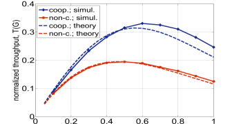
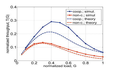
Figure 3: Normalized throughput $T(G)$ versus the normalized load $G=np/m$, for the average user’s degree $\lambda=3$ (top) and $\lambda=6$ (bottom).

References

- [1] G. L. Roberts, “ALOHA packet system with and without slots and capture,” SIGCOMM Comput. Commun. Rev., vol. 5, no. 2, April 1975.
- [2] H. Okada, Y. Igarashi, and Y. Nakanishi, “Analysis and application of framed ALOHA channel in satellite packet switching networks – FADRA method,” Electr. Comm. Japan, vol. 60, pp. 72–80, Aug. 1977.
- [3] E. Casini, R. De Gaudenzi, and O. del rio Herrero, “Contention resolution diversity slotted ALOHA (CRDSA): An enhanced random access scheme for satellite access packet networks,” IEEE Transactions on Wireless Communications, vol. 6, no. 4, pp. 1408–1419, April 2007.
- [4] G. Liva, “Graph-based analysis and optimization of contention resolution diversity slotted ALOHA,” IEEE Transactions on Communications, vol. 59, no. 2, pp. 477–487, February 2011.
- [5] C. Stefanovic, P. Popovski, and D. Vukobratovic, “Frameless aloha protocol for wireless networks,” IEEE Commun. Lett., vol. 16, no. 12, pp. 2087– 2090, 2012.
- [6] G. L. Choudhury and S. S. Rappaport, “Diversity ALOHA – a random access scheme for satellite communications,” IEEE Transactions on Communications, vol. 31, no. 2, pp. 450–457, 1983.
- [7] M. Zorzi, “Mobile radio slotted ALOHA with capture, diversity and retransmission control in the presence of shadowing,” Wireless Networks, vol. 4, pp. 379–388, August 1998.
- [8] A. Munari, M. Heindlmaier, G. Liva, and M. Berioli, “The throughput of slotted aloha with diversity,” in st Annual Allerton Conf. on Comm., Contr., and Comp., Monticello, IL, Oct. 2013.
- [9] M. Luby, M. Mitzenmacher, and A. Shokrollahi, “Analysis of random processes via and-or tree evaluation,” in 9th Annual ACM-SIAM Symp. Discr. Algorithms, San Francisco, CA, Jan. 1998, pp. 561 –568.
- [10] M. Luby, M. Mitzenmacher, A. Shokrollahi, and D. Spielman, “Efficient erasure correcting codes,” IEEE Trans. Inf. Theory, vol. 47, no. 2, pp. 569–584, 2001.