Inflection point analysis for Greek seismicity 1900-2006

Abstract

The seismicity of Greek region is studied under the prism of ESE & EDE methods for finding the inflection point of cumulative energy released. Main shocks are chosen from 106 years data. The result is that with both methods a critical time region exist at the end of 1982 to early 1983. After this time the seismicity tends to increase and gives remarkable events, like Athens Sep 1999 earthquake.

MSC2000. Primary 86A15, Secondary 65H99
Keywords. ESE, EDE, inflection point, seismic energy, Greek seismicity, earthquake.

1 Description of data used

We are using data from Seismic Hazard Harmonization in Europe project, see  [1], which has an index to show that an event is a main one and not an aftershock one. We are interested to study only main events, so the above data is extremely useful. We have removed from data the entries without a valid magnitude value. We have also focused our data at the region of Longitude East $(19.5000^{o},28.9984^{o})$ and Latitude North $(34.8024^{o},41.9943^{o})$.
The description of our data is presented at Table 1. By using  [2] we present the density plot of all main events at Figure 1. The counting of events region by region is presented at Figure 2. We clearly observe the main Greek seismicity arc where bigger events usually take place.

Table 1: Descriptive statistics of Magnitude, main events, 1900-2006

Statistic	N	Mean	St. Dev.	Min	Max
Magnitude	2,227	4.744	0.597	4.000	7.700

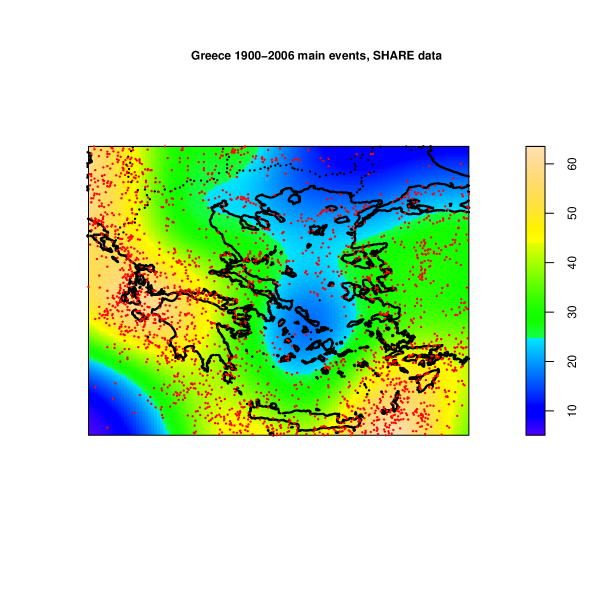
Figure 1: Density plot of main events in Greece, 1900 - 2006

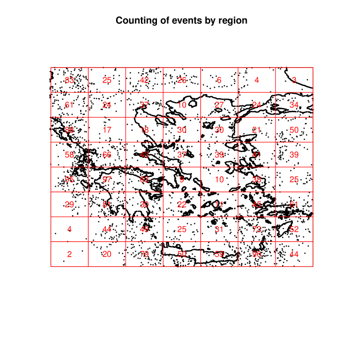
Figure 2: Counting of main events by region in Greece, 1900 - 2006

2 Inflection point analysis

In order to examine the cumulative energy that is released from main events we just simply compute the cumulative sum of the Magnitudes which is a good index for it. If we plot it versus time we observe that it has an interesting shape, see Figure 3.
We want to investigate which time is the inflection point in this plot in order to see if there exists a significant increase in the released seismic energy. For this purpose we are going to use the methods ESE & EDE, as described theoretically in  [3] and as implemented in R Package inflection, see  [4]. The ESE iterations are at Table 2 while the EDE iterations are in Table 3 and the relevant plot at Figure 4.

Table 2: ESE iterations for inflection point of cumulative magnitude

	#1	#2	#3	#4	#5
ESE iters	1992.10	1981.22	1983.56	1982.66	1983.11

Table 3: EDE iterations for inflection point of cumulative magnitude

	#1	#2	#3	#4
EDE iters	1985.63	1984.48	1983.89	1982.69

Table 4: ESE & EDE first application for cumulative magnitude

	$i_{1}$	$i_{2}$	$\chi$
ESE	1977.37	2006.84	1992.10
EDE	1964.26	2007.00	1985.63

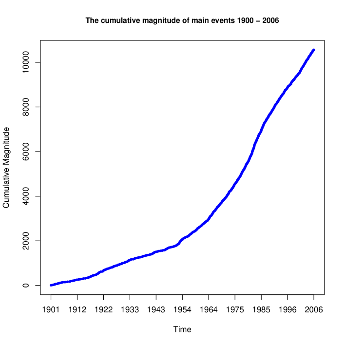
Figure 3: Cumulative Magnitude in Greece, 1900 - 2006

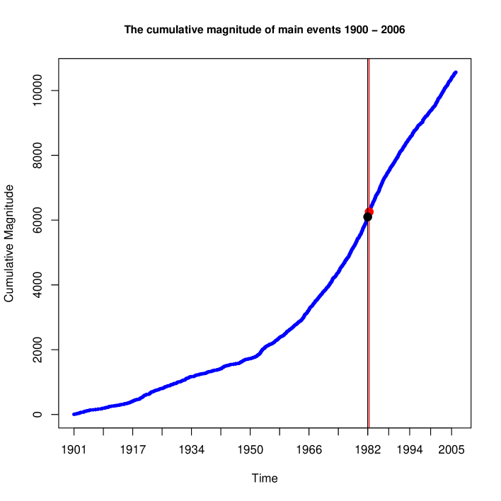
Figure 4: Inflection point in Cumulative Magnitude in Greece, 1900 - 2006

If we focus on the intervals that locate the inflection point from the first application of our methods we see from Table 4 that we have a change from mid ’60’s to mid ’70’s which is also directly observable at Figures 3 & 4. The fact that the second time is exactly the end of time interval on consideration means that we have not a complete sigmoid curve yet.
From the mass-energy equivalence in Mechanics we could treat the released energy (as measured by magnitude $M_{i}$) of a main event locally to represent an equivalent of a mass. By taking into account the depth $d_{i}$ of the event we can compute the quantities:

$$\begin{matrix}I^{(0)}=M_{i}\,d_{i}^{0}\\ I^{(1)}=M_{i}\,d_{i}^{1}\\ I^{(2)}=M_{i}\,d_{i}^{2}\\ \vdots\\ I^{(n)}=M_{i}\,d_{i}^{n}\\ \end{matrix}$$ (1)

We can call the above quantities ‘generalised inertia moments’ (GIM) of the seismic events, since for $i=2$ it is just the inertia moment of a mass that rotates around an axis in a distance $d_{i}$. We continue by computing the relative cumulative GIM for $n=0,1,2,\ldots\,5$. The descriptive statistics of Magnitude and Depth that have been used is presented at Table 5

Table 5: Descriptive statistics of Magnitude and Depth, main events, 1900-2006

Statistic	N	Mean	St. Dev.	Min	Max
Magnitude	2,188	4.737	0.583	4.000	7.700
Depth	2,188	33.744	31.800	1	199

We plot now the GIM at Figure 5, after normalising to the interval $[0,1]$ for comparison reasons. At the same plot we have marked the iterative ESE inflection point. We see that all inflection points are identical and very close to that of the single cumulative magnitude of Figure 4.

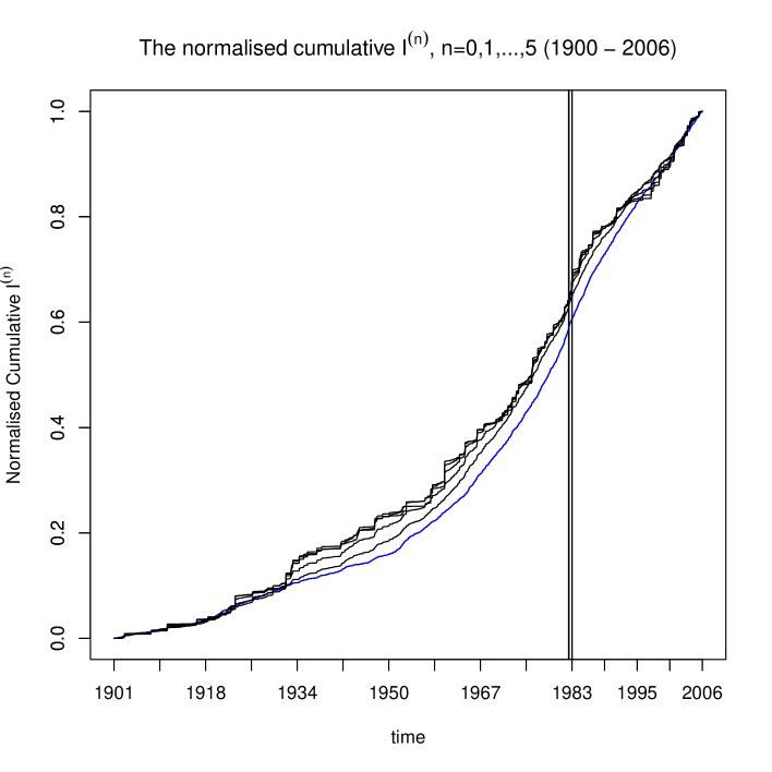
Figure 5: Normalised cumulative $I^{(n)},n=0,1,\ldots,5$ in Greece, 1900 - 2006

Let’s try now to add all GIM and obtain the Total GIM (TGIM) for each event

$$TI^{(n)}=\sum_{i=0}^{n}{I^{(n)}}$$ (2)

We are computing the TGIM and the relevant inflection point of it, after normalising to unity. Results are plotted at Figure 6. We don’t see any remarkable deviation for the inflection point.

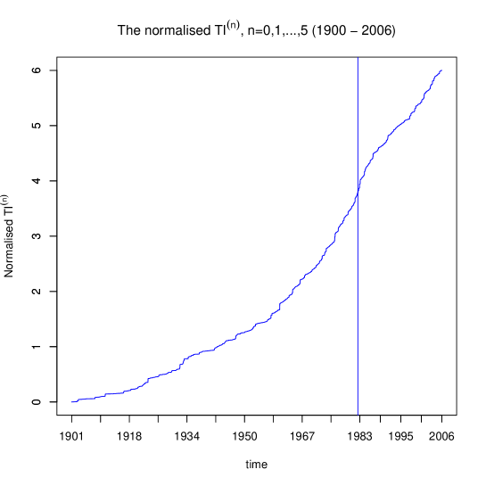
Figure 6: Normalised cumulative $TI^{(n)},n=0,1,\ldots,5$ in Greece, 1900 - 2006

3 Discussion

Although the magnitude of an earthquake is a measure of the deformation we tried to investigate the situation by introducing the ‘generalised inertia moments’ for every event. Our motivation was that of a Taylor series expansion: Why not to consider all the powers of a reasonable series like that which contains the moment of inertia? By using iterative ESE & EDE methods we observed that a time inflection point exist at the end of 1982 to the beginning of 1983. Further investigation is needed for the use of cumulative quantities in describing seismological data.

References

- [1] SHARE, Seismic Hazard Harmonization in Europe, in http://www.share-eu.org/, 2013.
- [2] Adrian Baddeley and Rolf Turner spatstat: An R Package for Analysing Spatial Point Patterns. Journal of Statistical Software 12(6), 1-42. URL http://www.jstatsoft.org/v12/i06/.
- [3] D. T. Christopoulos, Developing methods for identifying the inflection point of a convex/concave curve, in arXiv:1206.5478 [math.NA], http://arxiv.org/abs/1206.5478, 2012.
- [4] D. T. Christopoulos, R package inflection: Finds the inflection point of a curve, in http://CRAN.R-project.org/package=inflection, 2013.