Nonparametric gamma kernel estimates of density derivatives on positive semi-axis

Abstract

:  We consider nonparametric estimation of the derivative of a probability density function with the bounded support on $[0,\infty)$. Estimates are looked up in the class of estimates with asymmetric gamma kernel functions. The use of gamma kernels is due to the fact they are nonnegative, change their shape depending on the position on the semi-axis and possess other good properties. We found analytical expressions for bias, variance, mean integrated squared error (MISE) of the derivative estimate. An optimal bandwidth, the optimal MISE, and rate of mean square convergence of the estimates for density derivative have also been found.

1 Introduction

In many models of financial and actuary mathematics variables can be only positive. That is why the proposal of adequate methods for estimating characteristics of these models is up to date. In the paper of Song Xi Chen:20 nonparametric gamma kernel estimate for a reconstruction of probability density functions $f(x)$ with support $[0,\infty)$ was proposed. As it is known, for instance, from Jones:95 classical estimation methods with symmetric kernels yield a large bias on the zero boundary that leads to a bad quality of classical estimates in this case. In contrast to it, nonparametric estimates with asymmetric gamma kernel have a small bias on the boundary near zero and have a variance at a point $x$ of order $O(n^{-4/5}x^{-1/2})$, which decreases with the increase of the argument $x$. Such good properties of the estimates induce one to use them as a basis for the synthesis and investigation of the density derivative estimates. One of the important areas of application for density derivative estimates is the theory of nonparametric signal estimation, published in Dobrovidov:12, where these results are finely used, for example, in multiplicative stochastic models. Equation for the optimal signal estimate are expressed in terms of the logarithmic density derivative of the observed random variables which is known to contain a density derivative. Thus, the construction and investigation of a nonparametric kernel estimate of the density derivative function is the goal of this work.

2 Main results

Let $X_{1}...X_{n}$ be a sample of i.i.d random variables from a distribution with an unknown probability density function $f(x)$, which is defined on the support $x\in[0,\infty)$. The gamma kernel estimate is defined in Song Xi Chen:20 as

$$\hat{f}(x)=\frac{1}{n}\sum_{i=1}^{n}K_{\rho_{b}(x),b}(X_{i}),$$ (1)

where

$$K_{\rho_{b}(x),b}(t)=\frac{t^{\rho_{b}(x)-1}\exp(-t/b)}{b^{\rho_{b}(x)}\Gamma(\rho_{b}(x))}.$$

Here $b\rightarrow 0$ is a smoothing parameter (bandwidth), $\Gamma(\cdot)$ is a standard gamma function and

$$\rho_{b}(x) = \left\{\begin{array}[]{ll}\rho_{1}(x)=\frac{x}{b},&\mbox{if}\qquad x\geqslant 2b,\\ \rho_{2}(x)=\left(\frac{x}{2b}\right)^{2}+1,&\mbox{if}\qquad x\in[0,2b).\end{array}\right.$$

The support of the gamma kernel matches the support of the probability density function to be estimated. For convenience let us introduce two kernel functions

$$K_{\rho_{1}(x),b}(t) =\frac{t^{x/b-1}\exp(-t/b)}{b^{x/b}\Gamma(x/b)},\quad \mbox{if}\qquad x\geqslant 2b,$$

$$K_{\rho_{2}(x),b}(t) =\frac{t^{(\frac{x}{2b})^{2}}\exp(-t/b)}{b^{(\frac{x}{2b})^{2}+1}\Gamma((\frac{x}{2b})^{2}+1)},\quad \mbox{if}\qquad x\in[0,2b).$$

The estimate $\hat{f}^{\prime}(x)$ for density derivative $f^{\prime}(x)=df(x)/dx$ is usually taken as derivative of $\hat{f}(x).$ Hence, we can write it as follows

$$\hat{f}^{\prime}(x)=\frac{1}{n}\sum_{i=1}^{n}K^{\prime}_{\rho_{b}(x),b}(X_{i}),$$ (3)

where

$$K^{\prime}_{\rho_{b}(x),b}(t)=$$

$$= \left\{\begin{array}[]{ll}K^{\prime}_{\rho_{1}(x),b}(t)=\frac{1}{b}K_{\rho_{1}(x),b}(t)L_{1}(t),&\mbox{if}\quad x\geqslant 2b,\\ K^{\prime}_{\rho_{2}(x),b}(t)=\frac{x}{2b^{2}}K_{\rho_{2}(x),b}(t)L_{2}(t),&\mbox{if}\quad x\in[0,2b),\end{array}\right.$$

with

$$L_{1}(t)=L_{1}(t;x)=\ln t-\ln b-\Psi(\rho_{1}(x)),$$

$$L_{2}(t)=L_{2}(t;x)=\ln t-\ln b-\Psi(\rho_{2}(x)).$$

Here $\Psi(x)$ denotes Digamma function (logderivative of gamma function).

Now we get down to examine the properties of the derivative estimate (3). First of all, we investigate the expectation $\mathsf{E}(\hat{f}^{\prime}(x)).$ It should be noted that each class of estimates has nice properties only for a special class of densities. For instance, the estimates proposed by Song Xi Chen:20 are matched to a class of densities, satisfying the conditions: $f$ has a continuous second derivative, and the integrals $\int_{0}^{\infty}f^{\prime 2}(x)dx,$ $\int_{0}^{\infty}\{xf^{\prime\prime}(x)\}^{2}dx$ and $\int_{0}^{\infty}x^{-3/2}f(x)dx$ are finite. We intend to get analogous conditions for the density derivative estimate (3).

Lemma 1.(expectation) If  $b\rightarrow 0$ then the leading term of the mathematical expectation expansion for the density derivative estimate (3) equals

$$\mathsf{E}(\hat{f^{\prime}}(x))=\left\{\begin{array}[]{ll}\mathsf{E}K^{\prime}_{\rho_{1}(x),b}(X_{1}),&\mbox{if}\quad x\geqslant 2b,\\ \mathsf{E}K^{\prime}_{\rho_{2}(x),b}(X_{1}),&\mbox{if}\quad x\in[0,2b),\end{array}\right.$$

where

$$\begin{array}[]{ll}&\mathsf{E}K^{\prime}_{\rho_{1}(x),b}(X_{1})=(1/b)\mathsf{E}K_{\rho_{1}(x),b}(X_{1})L_{1}(X_{1};x)\\ &=f^{\prime}(x)+b\left(\frac{1}{12x^{2}}f(x)+\frac{1}{4}f^{\prime\prime}(x)\right)+o(b),\\ &\mathsf{E}K^{\prime}_{\rho_{2}(x),b}(X_{1})=(x/2b^{2})\mathsf{E}K_{\rho_{2}(x),b}(X_{1})L_{2}(X_{1};x)\\ &=f^{\prime}(x)\left(\frac{x}{2b}-\frac{b}{6x}\right)+f^{\prime\prime}(x)\left(\frac{7x}{48}+\frac{x^{2}}{2b}\right)+o(b).\end{array}$$

The proof of the Lemma 1 one can find in the Appendix. Note that under fixed $b$ the estimate $\hat{f^{\prime}}(x)$ in the small area $x\in[0,2b)$ near zero has a bias, which grows as $x\rightarrow 0$ . However, in the asymptotic case when $b\rightarrow 0$ the right boundary of this area $x=2b$ decreases also to zero. Therefore, it is interesting to know the bias limit when $x$ and $b$ converge to zero simultaneously, i.e. when ratio $x/b$ tends to some constant $\kappa$ when $b\rightarrow 0$. Then the second expectation of the estimate will differ very small from the true density derivative. The leading term of bias expansion may be written as

$$Bias(\hat{f}^{\prime}(x)) = b\left(\frac{f(x)}{12x^{2}}+\frac{f^{\prime\prime}(x)}{4}\right)+o(b),\quad i\!f\;x/b\rightarrow\infty,$$

$$Bias(\hat{f}^{\prime}(x)) = f^{\prime}(x)\left(\frac{3\kappa^{2}-6\kappa-1}{6\kappa}\right)$$

$$+ bf^{\prime\prime}(x)\left(\frac{7\kappa}{48}+\frac{\kappa^{2}}{2}\right)+o(b),\quad i\!f\;x/b\rightarrow\kappa.$$

If $x=2b$ then $\kappa=2$ and the estimate bias in the right boundary of the small area near zero will differ from true density derivative in $(1/12)f^{\prime}(2b)$.

As a global performance of the density derivative estimate (3) we select a mean integrated squared error ($MISE$), which, as is known, equals to

$$MISE(\hat{f}^{\prime}(x)) = \mathsf{E}\int\limits_{0}^{\infty}(f^{\prime}(x)-\hat{f}^{\prime}(x))^{2}dx$$

$$= \int\limits_{0}^{\infty}\big{[}Bias^{2}(\hat{f}^{\prime}(x))+Var(\hat{f}^{\prime}(x))\big{]}dx.$$

As the right boundary $x=2b$ decreases with $n\rightarrow\infty,$ then the integral contribution to $MISE$ of the second part of the bias in a small area near zero will be negligible. Hence, the integral squared bias of the main area of support is important only. Here it is

$$IBias^{2}(\hat{f^{\prime}}(x)) = \frac{b^{2}}{16}\int_{0}^{\infty}\left(\frac{f(x)}{3x^{2}}+f^{\prime\prime}(x)\right)^{2}dx+o(b^{2}).$$

Let us proceed to calculate the variance of the derivative estimate.

Lemma 2.(variance) If  $b\rightarrow 0$ and $nb^{3/2}\rightarrow\infty,$ then the leading term of variance expansion for density derivative estimate (3) equals to

$$Var(\hat{f}^{\prime}(x))=$$

$$= \frac{n^{-1}b^{-3/2}x^{-1/2}}{2\sqrt{\pi}}\left(\frac{f(x)}{2x}+b\left(\frac{f(x)}{4x^{2}}-\frac{f^{\prime}(x)}{4x}\right)\right)+o(b)$$

The proof of the Lemma 2 is in the Appendix.

The next problem is to calculate the mean squared error $MSE(x)$ in accordance to the well known formula. Then

$$MSE\left(\hat{f}^{\prime}(x)\right)=\frac{b^{2}}{16}\left(\frac{f(x)}{3x^{2}}\!\!\!\!+\!f^{\prime\prime}(x)\right)^{2}+\frac{n^{-1}b^{-3/2}x^{-1/2}}{2\sqrt{\pi}}$$

$$\cdot \left(\frac{f(x)}{2x}+b\left(\frac{f(x)}{4x^{2}}-\frac{f^{\prime}(x)}{4x}\right)\right)+o(b^{2}),$$

where

$$P(x)=\left(\frac{f(x)}{3x^{2}}+f^{\prime\prime}(x)\right)^{2},$$

If $P(x)\neq 0$, then minimization $MSE(x,b)=MSE\left(\hat{f}^{\prime}(x)\right)$ in $b$ provides an asymptotically optimal value of $b$

$$b_{opt}(x)=A(x)n^{-2/7},$$ (7)

where the so called initial coefficient $A(x)$ equals

$$A(x)=\left(\frac{3f(x)x^{-\frac{3}{2}}}{\sqrt{\pi}P(x)}\right)^{\frac{2}{7}}\!\!\!\!\!\!.$$

The bandwidth $b_{opt}(x)$ cannot be calculated directly because it depends on the unknown true density $f(x).$ An algorithm for evaluation $b_{opt}$ based on observations only will be presented in the next paper.

Substituting $b_{opt}(x)$ in $MSE\left(\hat{f}^{\prime}(x)\right)$ leads to the asymptotically optimal mean squared error of the estimate $\hat{f}^{\prime}_{1}(x)$ in each point $x$:

$$MSE_{opt}(\hat{f}^{\prime}(x))=\frac{A(x)^{2}P(x)^{2}}{16}n^{-\frac{4}{7}}+\frac{x^{-\frac{3}{2}}A(x)^{-\frac{3}{2}}}{4\sqrt{\pi}}n^{-\frac{4}{7}}.$$

Now we proceed to global performance (2). We will receive the integrated optimal bandwidth which doesn’t depend on $x.$

Theorem ($MISE$). If $b\rightarrow 0$ and  $nb^{3/2}\rightarrow\infty,$ integrals

$$\int_{0}^{\infty}\!\!\!\left(\frac{f(x)}{3x^{2}}+f^{\prime\prime}(x)\right)^{2}\!\!\!dx,\int_{0}^{\infty}\!\!\!\!\!x^{-3/2}f(x)dx$$

are finite and $\int_{0}^{\infty}P(x)dx\neq 0$, then the leading term of a MISE expansion for the density derivative estimate $\hat{f}^{\prime}(x)$ equals to

$$MISE(\hat{f}^{\prime}(x))=\frac{b^{2}}{16}\int_{0}^{\infty}\left(\frac{f(x)}{3x^{2}}+f^{\prime\prime}(x)\right)^{2}dx$$

$$+ \!\!\int_{0}^{\infty}\frac{n^{-1}b^{-3/2}x^{-3/2}}{4\sqrt{\pi}}\left(f(x)+\frac{b}{2}\left(\frac{f(x)}{x}-f^{\prime}(x)\right)\right)dx$$

$$+ o(b^{2}+n^{-1}b^{-3/2}).$$

Minimization of (2) in $b$ leads to a global optimal bandwidth

$$b_{0}=\left(\frac{3\int_{0}^{\infty}x^{-3/2}f(x)dx}{\sqrt{\pi}\int_{0}^{\infty}(\frac{f(x)}{3x^{2}}+f^{\prime\prime}(x))^{2}dx}\right)^{2/7}n^{-2/7},$$ (9)

whose substitution into (2) results to an optimal $MISE$

The restrictions on the integrals in the Theorem are fulfilled, for example, for the family of $\chi^{2}$-distributions with a number of degrees of freedom $m\geqslant 3.$ For $m=3$ we receive Maxwell distribution, which will be investigated as true distribution in simulation below.

From expression for $MISE_{opt}$ it follows that nonparametric estimate (3) converges in mean square to true density derivative with the rate $O(n^{-4/7}).$ This rate is certainly less than the rate of convergence for the density $O(n^{-4/5})$, because the estimation of derivatives is more complex than the estimation of the densities. A similar decrease in the rate of convergence for the derivatives compared with the densities was observed in the use of Gaussian kernel functions on the whole line.

3 Simulation results

In the simulation experiment we select the density of Maxwell distribution with parameter $\sigma=1$ as the true density to be estimated:

$$f_{M}(x)=\frac{\sqrt{2}x^{2}\exp(-\frac{x^{2}}{2\sigma^{2}})}{\sigma^{3}\sqrt{\pi}}.$$

We need two derivatives of it for computation integrals in the optimal bandwidth $b_{0}$ (9)

$$f^{\prime}_{M}(x)=-\frac{\sqrt{2}x\exp(-\frac{x^{2}}{2\sigma^{2}})(x^{2}-2\sigma^{2})}{\sigma^{5}\sqrt{\pi}},$$

$$f^{\prime\prime}_{M}(x)=\frac{\sqrt{2}\exp(-\frac{x^{2}}{2\sigma^{2}})(2\sigma^{4}-5\sigma^{2}x^{2}+x^{4})}{\sigma^{7}\sqrt{\pi}}.$$

Sample sizes are $n=200$ and $n=2000$. For comparison, the values of bandwidths were determined by three methods. The first calculates bandwidth from the formula (9). It has two integrals where we have to substitute $f_{M}(x)$ and its derivatives instead of $f(x)$ with corresponding derivatives. For $\sigma=1$ and $n=2000$ the values of the integrals are:
in numerator

$$\left(\frac{3}{\sqrt{\pi}}\int_{0}^{\infty}x^{-3/2}f_{M}(x)dx\right)^{2/7}=1.099,\qquad n^{-2/7}=0.114;$$

in denominator

$$\left(\int_{0}^{\infty}\left(\frac{f_{M}(x)}{3x^{2}}+f^{\prime\prime}_{M}(x)\right)^{2}dx\right)^{2/7}=1.247.$$

Combining these data together, we obtain $b_{1}=0.1004$.
The second bandwidth is a solution of equation (LABEL:11), where the integral coefficients were calculated numerically. The coefficient of $b$ is

$$\frac{1}{8}\left(\int_{0}^{\infty}(\frac{f_{M}(x)}{3x^{2}}+f^{\prime\prime}_{M}(x))^{2}dx\right)^{2}=0.270.$$

The coefficients of $b^{-5/2}$ and $b^{-3/2}$ are, respectively,

$$\frac{3n^{-1}}{8\sqrt{\pi}}\!\int_{0}^{\infty}\!\!\!x^{-\frac{3}{2}}f_{M}(x)dx=8.69\cdot 10^{5},$$

$$\frac{n^{-1}}{16\sqrt{\pi}}\!\int_{0}^{\infty}\!\!\!x^{-\frac{3}{2}}\left(\frac{f_{M}(x)}{x}-f_{M}^{\prime}(x)\right)dx=-2.69\cdot 10^{5}.$$

Substitution all of them in (LABEL:11) yields the transcendental equation

$$0.270b+8.69\cdot 10^{5}b^{-5/2}-2.69\cdot 10^{5}b^{-3/2}=0,$$

which can be solved by numerical methods. Solution of it provides $b_{2}=0.1013$.

The third $b_{3}$ was taken from the paper of Song Xi Chen (2000), where he found an optimal in mean square sense bandwidth

$$b_{3}=\left(\frac{V}{\beta}\right)^{2/5}n^{-2/5},$$

where

$$V=\frac{1}{2\sqrt{\pi}}\int\limits_{0}^{\infty}x^{-1/2}f_{M}(x)dx,\quad\beta=\int\limits_{0}^{\infty}(xf_{M}^{\prime\prime}(x))^{2}dx\neq 0.$$

In our case it is equals to $b_{3}=0.0175$. In this case one might think that if the estimate of the derivative of density is constructed as a derivative of the density estimate, then the best bandwidth for the density will be good for its derivative. However, this is not the case, as evidenced by the experimental results.

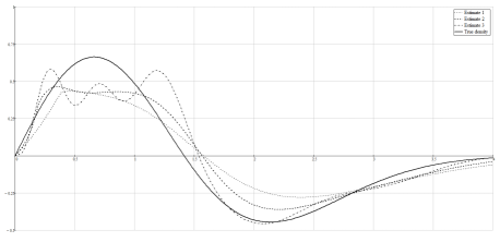
Figure 1: Nonparametric estimates of Maxwell density derivative function for n=200. The $f^{\prime}_{M}(x)$ (solid line), estimate 1 b1=0.194 (dotted line), estimate 2 b2=0.197 (dashed line), estimate 3 b3=0.0175 (dash-dotted line).

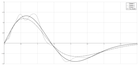
Figure 2: Nonparametric estimates of Maxwell density derivative function for n=2000. The $f^{\prime}_{M}(x)$ (solid line), estimate 1 b1=0.1004 (dotted line), estimate 2 b2=0.1013 (dashed line), estimate 3 b3=0.0175 (dash-dotted line).

From Fig. 1 and Fig. 2 it is visible that the estimate 1 and 2 areclose to the desire density derivative (solid line). The estimate 2 is quite smooth compared with the estimate 3 using the optimal bandwidth $b_{3}$ for the density. This is confirmed by the numerical evaluation of the squared integral deviation from the true derivative curve, as it is shown in the table.

Table 1:

Deviation of estimates

Bandwidth	$b_{1}$	$b_{2}$	$b_{3}$
Value	0.203	0.146	0.017
Deviation	0.0426	0.0382	0.0450

The estimate 2 with $b_{2}$, when we solve a transcendental equation, provides the best result. If there are multiple roots of the transcendental equation, we choose the root with the lowest value of $MISE$.

4 Conclusions

We have developed a method of nonparametric density derivative estimation on the positive semi-axis, which is supposed to be applied to nonlinear problems of signal selection with unknown characteristics from the mixture with noise. Such problems are arisen in the theory of nonparametric estimation of signals with unknown distribution, where there is an equation of optimal filtering, containing statistics in the form of the logarithmic derivative of the density. In multiplicative observation models with positive signals the logarithmic derivative has to be reconstructed from observations. Since the logarithmic derivative contains a derivative of the unknown density, the presented method for estimating the derivative is relevant.

This method is expected to be extended to dependent variables. In addition, since the optimal bandwidth depends on the unknown density, it is necessary to build its data-based estimate and thus to create an automatic technique of nonparametric signal estimation.

Appendix: PROOFS OF THE STATEMENTS.

Proof of Lemma 1.

We start by writing the expectation of the estimate (3) on the both intervals of the support.
1) For the interval $x\geqslant 2b$

$$\mathsf{E}(\hat{f}^{\prime}(x))=\int_{0}^{\infty}\frac{1}{b}K_{\rho_{1},b}(y)L_{1}(y;x)f(y)dy$$ (10)

$$= \mathsf{E}\left(b^{-1}(\ln\xi_{x}-\ln b-\Psi(\rho_{1}))\cdot f(\xi_{x})\right)$$

$$= \frac{1}{b}[\mathsf{E}(\ln\xi_{x}\cdot f(\xi_{x}))-(\ln b+\Psi(\rho_{1}))\mathsf{E}(f(\xi_{x}))],$$

where $\xi_{x}$ is a $\text{Gamma}(\rho_{1},b)$ random variable. From the standard theory of gamma distribution it is known that for this random variable mean is $\mu_{x}=\mathsf{E}(\xi_{x})=\rho_{1}b$ and variance is $Var_{1}(\xi_{x})=\rho_{1}b^{2}$.
2) Regarding the interval $x\in[0,2b)$ we get in a similar way:

$$\mathsf{E}(\hat{f^{\prime}}(x))=\int_{0}^{\infty}K_{\rho_{2},b}(y)L_{2}(y;x)\frac{x}{2b^{2}}f(y)dy$$ (11)

$$= \frac{x}{2b^{2}}\mathsf{E}((\ln\eta_{x}-\ln b-\Psi(\rho_{2}))\cdot f(\eta_{x}))$$

$$= \frac{x}{2b^{2}}[\mathsf{E}(f(\eta_{x})\ln\eta_{x})-(\ln b+\Psi(\rho_{2})\cdot\mathsf{E}(f(\eta_{x}))],$$

where $\eta_{x}$ is a $\text{Gamma}(\rho_{2},b)$ random variable with mean $\mu_{x}=\mathsf{E}(\eta_{x})=\rho_{2}b$ and variation $Var_{2}(\eta_{x})=\rho_{2}b^{2}$. Up to a factor, it is the same as in (10). Then we will make the Taylor series expansion at a point $\mu_{x}$ for general $\rho$ and then substitute in the appropriate cases $\rho_{1}$ or $\rho_{2}$. Consider the first term in (10),(11):

$$\mathsf{E}(f(\xi_{x})\ln\xi_{x})=\mathsf{E}(f(\mu_{x})\ln\mu_{x})$$

$$+ \mathsf{E}((f(\mu_{x})\ln\mu_{x})^{\prime}(\xi_{x}-\mu_{x}))$$

$$+ \frac{1}{2}\mathsf{E}((f(\mu_{x})\ln\mu_{x})^{\prime\prime}(\xi_{x}-\mu_{x})^{2})+o(b)$$

$$= f(\mu_{x})\ln\mu_{x}+\frac{Var(\xi_{x})}{2}$$

$$\cdot \left(\frac{2f^{\prime}(\mu_{x})}{\mu_{x}}+f^{\prime\prime}(\mu_{x})\ln(\mu_{x})-\frac{f(\mu_{x})}{\mu_{x}^{2}}\right)+o(b).$$

We substitute the mean and variance by their values from a gamma distribution:

$$f(\rho b)(\ln(\rho b)\!-\frac{1}{2\rho})\!+\!f^{\prime}(\rho b)b\!+\!f^{\prime\prime}(\rho b)\ln(\rho b)\frac{(\rho b)^{2}}{2}+o(b)$$

$$= f(x)\!\left(\ln(\rho b)\!-\frac{1}{2\rho}\right)\!+\!f^{\prime}(x)\left(\!\!\left(\ln(\rho b)-\frac{b}{2}\right)(x-\rho b)+b\!\right)$$

$$+ f^{\prime\prime}(x)\left(\left(\ln(\rho b)-\frac{1}{2\rho}\right)\frac{(x-\rho b)^{2}}{2}+b(x-\rho b)\right.$$

$$+ \left.\ln(\rho b)\frac{(\rho b)^{2}}{2}\right)+o(b).$$

The second term in (10)(11) can be represented just like above

$$\mathsf{E}(f(\xi_{x}))\!=\!f(x)+f^{\prime}(x)(x-\rho b)\!+\!f^{\prime\prime}(x)\!\left(\!\frac{\rho b^{2}}{2}\!+\!\frac{(x-\rho)^{2}}{2}\!\right)$$

$$+ o(b).$$

Then, combining all items in the square brackets in (10),(11), we can get

$$[f(x)\left(\ln(\rho b)-\frac{1}{2\rho}-(\ln b+\Psi(\rho))\right)$$

$$+ \!f^{\prime}(x)\!\left(\!\!\left(\ln(\rho b)-\frac{1}{2\rho}\right)\!(x-\rho b)+\!b-\!(\ln b+\Psi(\rho))(x\!-\rho b)\!\right)$$

$$+ \!f^{\prime\prime}(x)(\left(\ln(\rho b)-\frac{1}{2\rho}\right)\!\frac{(x-\rho b)^{2}}{2}\!+\!b(x-\rho b)+\ln(\rho b)\frac{(\rho b)^{2}}{2}$$

$$- (\ln b+\Psi(\rho))(\frac{\rho b^{2}}{2}+\frac{(x-\rho b)^{2}}{2}))+o(b)].$$

Using the approximation of the Digamma function when $\rho\rightarrow\infty$

$$\Psi(\rho) = \ln\rho-\frac{1}{2\rho}-\frac{1}{12\rho^{2}}+\frac{1}{120\rho^{4}}-\frac{1}{252\rho^{6}}+O\left(\frac{1}{\rho^{8}}\right),$$

we receive the expression in square brackets of (11) in $\rho$

$$[f(x)\left(\frac{1}{12\rho^{2}}\right)+f^{\prime}(x)\left(b+\frac{x-\rho b}{12\rho^{2}}\right)$$

$$+ \!f^{\prime\prime}(x)\!\left(\!\left(\!\frac{1}{2\rho}\!+\!\frac{1}{12\rho^{2}}\right)\frac{\rho b^{2}}{2}\!+\!\frac{(x-\rho b)^{2}}{24\rho^{2}}\!+b(x-\rho b)\!\right)\!+\!o(b)].$$

Now for cases 1) and 2) let us substitute $\rho_{1}$ and $\rho_{2}$ instead of $\rho$.
For 1):

$$\mathsf{E}(\hat{f}^{\prime}(x)) = \frac{1}{b}\left(f(x)\left(\frac{b^{2}}{12x^{2}}\right)+bf^{\prime}(x)+\frac{b^{2}}{4}f^{\prime\prime}(x)+o(b)\right)$$

$$= f^{\prime}(x)+b\left(\frac{1}{12x^{2}}f(x)+\frac{1}{4}f^{\prime\prime}(x)\right)+o(b).$$

For 2) we will use the fact that as $b\rightarrow 0$ then

$$\frac{1}{\rho}=\frac{4b^{2}}{x^{2}(1+\frac{4b^{2}}{x^{2}})}=\frac{4b^{2}}{x^{2}}+o(b^{2}),$$

and

$$\mathsf{E}(\hat{f^{\prime}}(x))=f^{\prime}(x)\left(\frac{x}{2b}-\frac{b}{6x}\right)+f^{\prime\prime}(x)\left(\frac{7x}{48}+\frac{x^{2}}{2b}\right)+o(b).$$

$$\Box$$

Proof of Lemma 2.

We start with variance for $x\geqslant 2b$.

$$Var(\hat{f}^{\prime}(x))=\frac{1}{n}Var(K^{\prime}_{\rho_{1},b}(x))$$ (12)

$$= \frac{1}{n}\big{(}\mathsf{E}(K^{\prime 2}_{\rho_{1},b}(x))-\mathsf{E}^{2}(K^{\prime}_{\rho_{1},b}(x))\big{)}.$$

The second term of the right-hand side of (12) is the same as in (10). So we can write immediately

$$\mathsf{E}^{2}(K^{\prime}_{\rho_{1},b}(x))=\left(f(x)\frac{b}{12x^{2}}+f^{\prime}(x)+f^{\prime\prime}(x)\frac{b}{4}+o(b)\right)^{2}.$$

The first term of the right-hand side of (12) can be represented by

$$\mathsf{E}(K^{\prime 2}_{\rho_{1},b}(x))=\int_{0}^{\infty}K^{\prime 2}_{\rho_{1},b}(y)f(y)dy$$

$$= \int_{0}^{\infty}\frac{y^{\frac{2x}{b}-2}\exp(\frac{-2y}{b})}{b^{\frac{2x}{b}}\Gamma^{2}(\frac{x}{b})}\left(\frac{L_{1}(y;x)}{b}\right)^{2}f(y)dy.$$

Using the property of the gamma function $\Gamma^{2}(\frac{x}{b}+1)=(\frac{x}{b})^{2}\Gamma^{2}(\frac{x}{b}),$ we get

$$\int_{0}^{\infty}\frac{y^{\frac{2x}{b}-2}\exp(\frac{-2y}{b})}{b^{\frac{2x}{b}}(\frac{b}{x})^{2}\Gamma^{2}(\frac{x}{b}+1)}\cdot\left(\frac{L_{1}(y;x)}{b}\right)^{2}f(y)dy$$

$$= \int_{0}^{\infty}\frac{b^{-5}x^{2}\Gamma(\frac{2x}{b}-1)}{2^{\frac{2x}{b}-2}\Gamma^{2}(\frac{x}{b}+1)}\frac{(2y)^{\frac{2x}{b}-2}\exp(\frac{-2y}{b})}{b^{\frac{2x}{b}-1}\Gamma^{(}\frac{2x}{b}-1)}$$

$$\cdot L_{1}(y;x)^{2}f(y)dy.$$

Denoting $B_{b}(x)=\frac{b^{-5}x^{2}\Gamma(\frac{2x}{b}-1)}{2^{\frac{2x}{b}-2}\Gamma^{2}(\frac{x}{b}+1)},$ it can be written shorter

$$= \int_{0}^{\infty}B_{b}(x)K_{\frac{2x}{b}-1,b}(y)L_{1}(t)^{2}f(y)dy$$ (13)

$$= B_{b}(x)\mathsf{E}(L_{1}(\eta_{x},x)^{2}f(\eta_{x})),$$

where $\eta_{x}$ is a Gamma$(\frac{2x}{b}-1,b)$ random variable with a mean $\mu_{x}=\mathsf{E}(\eta_{x})=2x-b$ and a variance $Var(\eta_{x})=2xb-b^{2}$. Let $R(z)=\sqrt{2\pi}\exp(-z)z^{z+1/2}/\Gamma(z+1)$ for $z\geqslant 0$. So we can express gamma function as

$$\Gamma^{2}(\frac{x}{b}+1) = \left(\frac{\sqrt{2\pi}\exp(\frac{-x}{b})(\frac{x}{b})^{\frac{x}{b}+1/2}}{R(\frac{x}{b})}\right)^{2}.$$

Using the properties of the gamma function

$$\Gamma(\frac{2x}{b}-1)=\frac{\Gamma(\frac{2x}{b}+1)}{\frac{2x}{b}(\frac{2x}{b}-1)}=\frac{\sqrt{2\pi}\exp(-\frac{2x}{b})(\frac{2x}{b})^{\frac{2x}{b}+\frac{1}{2}}}{\frac{2x}{b}(\frac{2x}{b}-1)R(\frac{2x}{b})},$$

we obtain

$$B_{b}(x)=\frac{b^{-5}x^{2}}{2^{\frac{2x}{b}-2}}\cdot\frac{1}{\frac{2x}{b}(\frac{2x}{b}-1)}\frac{\sqrt{2\pi}\exp(-\frac{2x}{b})(\frac{2x}{b})^{\frac{2x}{b}+\frac{1}{2}}}{R(\frac{2x}{b})}$$

$$\cdot \frac{R^{2}(\frac{x}{b})}{(\sqrt{2\pi})^{2}\exp(-\frac{2x}{b})(\frac{x}{b})^{\frac{2x}{b}+1}}=\frac{b^{-\frac{5}{2}}x^{-\frac{1}{2}}R^{2}(\frac{x}{b})}{\sqrt{\pi}R(\frac{2x}{b})(1-\frac{b}{2x})}.$$

According to Lemma 3 of Brown:99, $R(z)$ is increasing function which converges to 1 as $z\rightarrow\infty$ and $R(z)<1$ for any $z>0$.

Then

$$B_{b}(x) = \left\{\begin{array}[]{ll}\frac{b^{-5/2}x^{-1/2}}{2\sqrt{\pi}},&\mbox{if}\qquad\frac{x}{b}\rightarrow\infty,\\ \frac{b^{-3}k^{2}\Gamma(2k-1)}{2^{2k-2}\Gamma^{2}(k+1)},&\mbox{if}\qquad\frac{x}{b}\rightarrow k,\end{array}\right.$$

Let us denote $G=G(x,b)=\ln b+\Psi(\frac{x}{b})=\ln x-\frac{b}{2x}-\frac{b^{2}}{12x^{2}}+o(b^{2})$. Now we must find the second factor in (13)

$$\mathsf{E}(L_{1}(\eta_{x};x)^{2}f(\eta_{x}))=\mathsf{E}\left(\big{(}\ln\eta_{x}-\ln b-\Psi(\frac{x}{b})\big{)}^{2}f(\eta_{x})\right)$$

$$= \mathsf{E}(f(\eta_{x})\ln^{2}\eta_{x})-2G\mathsf{E}(f(\eta_{x})\ln\eta_{x})+G^{2}\mathsf{E}(f(\eta_{x})).$$

If $b/x\rightarrow 0,$ we can get Taylor series

$$\ln(2x-b) = \ln(2x(1-\frac{b}{2x}))=\ln(2x)+\ln(1-\frac{b}{2x})$$

$$= \ln(2x)-\frac{b}{2x}+o(b),$$

$$\frac{1}{2x-b}=\frac{1}{2x(1-\frac{b}{2x})}=\frac{1}{2x}+\frac{b}{4x^{2}}+o(b).$$

Substituting them in the expression above, we obtain

$$\mathsf{E}(f(\eta_{x})\ln^{2}\eta_{x})=f(\mu_{x})\ln^{2}\mu_{x}+(f(\eta_{x})\ln^{2}\eta_{x})^{\prime\prime}\frac{Var(\eta_{x})}{2}$$

$$= f(x)\ln^{2}(x)+b\Big{(}f^{\prime}(x)\left(\ln(x)-\frac{\ln^{2}(x)}{2}\right)$$

$$+ \frac{f(x)}{2x}\left(1-3\ln(x)\right)+f^{\prime\prime}(x)\frac{x\ln^{2}(x)}{4}\Big{)}$$

$$+ b^{2}\Big{(}f(x)\left(\frac{3}{4x^{2}}-\frac{\ln(x)}{2x^{2}}\right)+f^{\prime}(x)\frac{3}{4x}\left(\ln(x)-1\right)$$

$$+ f^{\prime\prime}(x)\left(\frac{\ln^{2}(x)}{8}-\frac{3\ln(x)}{4}\right)-f^{\prime\prime\prime}(x)\frac{x\ln^{2}(x)}{8}\Big{)}+o(b).$$

Similarly,

$$\mathsf{E}(f(\eta_{x})\ln\eta_{x})=f(\mu_{x})\ln\mu_{x}+(f(\eta_{x})\ln\eta_{x})^{\prime\prime}\frac{Var(\eta_{x})}{2}$$

$$= f(x)\ln(x)+b\Big{(}-f(x)\frac{3}{4x}+f^{\prime}(x)\frac{\left(1-\ln(x)\right)}{2}$$

$$+ f^{\prime\prime}(x)\frac{x\ln(x)}{4}\Big{)}+b^{2}\Big{(}-\frac{f(x)}{4x^{2}}f^{\prime}(x)\frac{3}{8x}$$

$$+ f^{\prime\prime}(x)\left(\frac{\ln(x)}{8}-\frac{3}{8}\right)-f^{\prime\prime\prime}(x)\frac{x\ln(x)}{8}\Big{)}+o(b),$$

$$\mathsf{E}(f(\eta_{x}))=f(\mu_{x})+f^{\prime\prime}(\mu_{x})\frac{Var(\xi_{x})}{2}$$

$$= f(x)-b\left(\frac{xf^{\prime\prime}(x)}{4}-\frac{f^{\prime}(x)}{2}\right)+b^{2}\left(\frac{f^{\prime\prime}(x)}{8}-\frac{xf^{\prime\prime\prime}(x)}{8}\right)+o(b).$$

Collecting all the terms, we obtain an expression

$$\mathsf{E}((\ln\eta_{x}-\ln b-\Psi(x/b))^{2}f(\eta_{x}))$$

$$= b\frac{f(x)}{2x}+b^{2}\left(\frac{f(x)}{4x^{2}}-\frac{f^{\prime}(x)}{4x}\right)+o(b).$$

Hence, as $b/x\rightarrow 0$, the variance is

$$Var(\hat{f}^{\prime}_{2}(x))=$$

$$= \frac{n^{-1}b^{-3/2}x^{-1/2}}{2\sqrt{\pi}}\left(\frac{f(x)}{2x}+b\left(\frac{f(x)}{4x^{2}}-\frac{f^{\prime}(x)}{4x}\right)\right).\quad\Box$$