Methods for Collision–Free Navigation of Multiple Mobile Robots in Unknown Cluttered Environments

Abstract

Navigation and guidance of autonomous vehicles is a fundamental problem in robotics, which has attracted intensive research in recent decades. This report is mainly concerned with provable collision avoidance of multiple autonomous vehicles operating in unknown cluttered environments, using reactive decentralized navigation laws, where obstacle information is supplied by some sensor system.

Recently, robust and decentralized variants of model predictive control based navigation systems have been applied to vehicle navigation problems. Properties such as provable collision avoidance under disturbance and provable convergence to a target have been shown; however these often require significant computational and communicative capabilities, and don’t consider sensor constraints, making real time use somewhat difficult. There also seems to be opportunity to develop a better trade-off between tractability, optimality, and robustness.

The main contributions of this work are as follows; firstly, the integration of the robust model predictive control concept with reactive navigation strategies based on local path planning, which is applied to both holonomic and unicycle vehicle models subjected to acceleration bounds and disturbance; secondly, the extension of model predictive control type methods to situations where the information about the obstacle is limited to a discrete ray-based sensor model, for which provably safe, convergent boundary following can be shown; and thirdly the development of novel constraints allowing decentralized coordination of multiple vehicles using a robust model predictive control type approach, where a single communication exchange is used per control update, vehicles are allowed to perform planning simultaneously, and coherency objectives are avoided.

Additionally, a thorough review of the literature relating to collision avoidance is performed; a simple method of preventing deadlocks between pairs of vehicles is proposed which avoids graph-based abstractions of the state space; and a discussion of possible extensions of the proposed methods to cases of moving obstacles is provided. Many computer simulations and real world tests with multiple wheeled mobile robots throughout this report confirm the viability of the proposed methods. Several other control systems for different navigation problems are also described, with simulations and testing demonstrating the feasibility of these methods.

Chapter 1 Introduction

1.1 Overview

Navigation of autonomous vehicles is an important, classic research area in robotics, and many approaches are well documented in the literature. However there are many aspects which remain an increasingly active area of research. A review of recently proposed navigation methods applicable to collision avoidance is provided in Chapt. 2.

Both single and coordinated groups of autonomous vehicles have many applications, such as industrial, office, and agricultural automation; search and rescue; and surveillance and inspection. All these problems contain some similar elements, and collision avoidance in some form is almost universally needed. Examples of compilations of potential applications may be readily found, see e.g. [338, 308].

In contrast to initial approaches to vehicle navigation problems, the focus in the literature has shifted to navigation laws which are capable of rigorous collision avoidance, such that for some set of assumptions, it can be proven collisions will never occur. Overall, navigation systems with more general assumptions would be considered superior. Some examples of common assumptions are listed as follows:

• Vehicle models vary in complexity from velocity controlled linear models to realistic car-like models (see Sec. 2.2). For example, collision avoidance for velocity controlled models is simpler since the vehicles can halt instantly if required; however this is physically unrealistic. This means a more complex model which better characterizes actual vehicles is desirable for use during analysis.

• Different levels of knowledge about the obstacles and other vehicles are required by different navigation strategies. This ranges from abstracted obstacle set information to allowance for the actual nature of realistic noisy sensor data obtained from range-finding sensors. In addition to the realism of the sensor model, the sensing requirements significantly varies between approaches – in some vehicle implementations less powerful sensors are installed, which would only provide limited information to the navigation system (such as the minimum distance to the obstacle).

• Different assumptions about the shape of static obstacles have been proposed. To ensure correct behavior when operating near an obstacle when only limited information is available, it is often unavoidably necessary to presume smoothness properties relating to the obstacle boundary. However, approaches which have more flexible assumptions about obstacles would likely be more widely applicable to real world scenarios.

• Uncertainty is always present in real robotic systems, and proving a behavior occurs under an exact vehicle model does not always imply the same behavior will be exhibited when the system is implemented. To better reflect this, assumptions can be made describing bounded disturbance from the nominal model, bounded sensor errors, and the presence of communication errors. A review of the types of uncertainty present in vehicle systems is available [66].

While being able prove collision avoidance under broad circumstances is of utmost importance, examples of other navigation law features which determine their effectiveness are listed as follows:

• Navigation laws which provably achieve the vehicle’s goals are highly desirable. When possible, this can be generally shown by providing an upper bound on the time in which the vehicle will complete a finite task, however conservative this may be. However, proving goal satisfaction is possibly less critical than collision avoidance, so long as it can be experimentally demonstrated non-convergence is virtually non-existent.

• In many applications, the computational ability of the vehicle is limited, and approaches with lower computational cost are favored. However, with ever increasing computer power, this concern is mainly focused towards small, fast vehicles such as miniature UAV’s (for which the fast update rates required are not congruent with the limited computational faculties available).

• Many navigation laws are constructed in continuous time. Virtually all digital control systems are updated in discrete time, thus navigation laws constructed in discrete time are more suitable for direct implementation.

The key distinction between different approaches is the amount of information they have available about the workspace. When full information is available about the obstacle set and a single vehicle is present, global path planning methods may be used to find the optimal path. When only local information is available, sensor based methods are used. A subset of sensor based methods are reactive methods, which may be expressed as a mapping between the sensor state and control input, with no memory present.

Recently, Model Predictive Control (MPC) architectures have been applied to collision avoidance problems, and this approach seems to show great potential in providing efficient navigation, and easily extends to robust and nonlinear problems (see Sec. 2.4). They have many favorable properties compared to the commonly used Artificial Potential Field (APF) methods and Velocity Obstacle based methods, which could be generally more conservative when extended to higher order vehicle models. MPC continues to be developed and demonstrate many desirable properties for sensor based navigation, including avoidance of moving obstacles (see Sec. 2.6), and coordination of multiple vehicles (see Sec. 2.7). Additionally, the use of MPC for sensor based boundary following problems has been proposed in this report (see Chapt. 4).

1.2 Chapter Outline

The problem statements and main contributions of each chapter are listed as follows:

• Chapt. 2 is based on [135], and presents a review of the literature relating to collision avoidance of static obstacles, moving obstacles, and other cooperating vehicles.

• Chapt. 3 is based on [134] and [136], and is concerned with the navigation of a single vehicle described by either holonomic or unicycle vehicle models with bounded acceleration and disturbance. Collision avoidance is able to be proven, however convergence to the target is not analytically addressed (since assumptions regarding sensor data are not particularly realistic). The contributions of this chapter are the integration of the robust MPC concept with reactive navigation strategies based on local path planning, applied to both holonomic and unicycle vehicle models with bounded acceleration and disturbance

• Chapt. 4 is based on [133], and is concerned with navigation in unknown environments where the information about the obstacle is limited to a discrete ray-based sensor model. Collision avoidance, complete transversal of the obstacle and finite completion time are able to be proven, however the vehicle model is assumed to be free from disturbance. To solve this problem, the MPC method from Chapt. 3 is extended to only consider the more limited obstacle information when performing the planning process.

• Chapt. 5 is based on [136], and is concerned with the navigation of multiple cooperating vehicles which are only allowed a limited number of communication exchanges per control update. Again, collision avoidance is able to be proven. To achieve this, a novel constraint is developed allowing decentralized robust coordination of multiple vehicles. Unlike other approaches in this area, explicit ordering of the vehicles is not required, each vehicle can plan trajectories simultaneously, and no explicit coherency objectives are required.

• Chapt. 6 is based on [132], and is concerned with preventing deadlocks between pairs of robots in cluttered environments. To achieve this, a simple yet original method of resolving deadlocks between pairs of vehicles is proposed. The proposed method has the advantage of not requiring centralized computation or discrete abstraction of the state space.

In Chapts. 3 to 6, simulations and real world testing confirm the viability of the proposed methods. It should be emphasized they are all related since they all use the same basic planning and collision avoidance procedure proposed in Chapt. 3.

In Chapts. 7 to 13, the contribution of the author was the simulations and testing performed to validate some other varieties of navigation systems. In each of these chapters, some of the introductory discussion, and all mathematical analysis, was contributed by coauthors to the associated manuscript; however some details are included to assist understanding of the presented results. Each of these chapters are relatively independent (they solve quite distinct problems), and some have introductions independent of Chapt. 2.

• Chapt. 7 is based on [223], and is concerned with reactively avoiding obstacles and provably converging to a target using only scalar measurements about the minimum distance to obstacles and the angle to the target. The advantage of the proposed method is that it can be analytically shown to have the correct behavior, despite the extremely limited sensor information which was assumed to be available.

• Chapt. 8 is based on [289], and is again concerned with reactively avoiding obstacles and provably converging to a target. However in contrast to Chapt. 7, the sensor information available is the set of visible obstacle edges surrounding the vehicle. The advantage of the proposed method is that it explicitly allows for the kinematics of the vehicle, compared to equivalent control approaches proposed in the literature.

• Chapt. 9 is based on [220], and is concerned with outlining in more detail the path following approach employed in Chapt. 3. In particular, extensive simulations and experiments with an agricultural vehicle are documented. The advantage of the proposed method is that it explicitly allows for steering angle limits, and it has been shown to have good tracking performance in certain situations compared to other methods proposed in the literature.

• Chapt. 10 is based on [224], and is concerned with following the boundary of an obstacle using limited range information. In contrast to Chapt. 4, only a single detection sector perpendicular to the vehicle is available. The advantage of the proposed method is that (compared to other equivalent methods proposed in the literature) it provides a single contiguous controller, and is analytically correct around transitions from concave to convex boundary segments.

• Chapt. 11 is based on [221], and is concerned with seeking the maximal point of a scalar environmental field. The advantage of the proposed method is that it des not require any type of derivative estimation, and it may be analytically proven to be correct in the case of time–varying environmental fields.

• Chapt. 12 is based on [219], and is concerned with tracking level sets/isolines of an environmental field at a predefined set-point. The advantage of the proposed method is that it may be analytically proven to be correct in the case of time–varying environmental fields.

• Chapt. 13 is based on [359], and is concerned with decentralized formation control allowing a group of robots to form a circular ‘capturing’ arrangement around a given target. The advantage of the proposed method is that it only requires local sensor information, allows for vehicle kinematics and does not require communication between vehicles.

Finally, Chapt. 14 presents a summary of the proposed methods, and outlines several areas of possible future research.

Appendix 15 presents preliminary simulations with a realistic helicopter model. Note the helicopter model and the text describing it was contributed by Dr. Matt Garratt.

Chapter 2 Literature Review

In this chapter both local and global approaches are reviewed, together with approaches applicable to multiple vehicles and moving obstacles. Various types of vehicle and sensor models are explored, and in the case of moving obstacles, various assumptions about their movement are discussed.

This chapter is structured as follows. In Sec. 2.2 the problem of navigating cluttered environments are described. In Sec. 2.4 MPC-based navigation systems are outlined. In Sec. 2.5 methods of sensor based navigation are introduced; in Sec. 2.6 methods of dealing with moving obstacles are reviewed. Sec. 2.7 deals with the case of multiple cooperating vehicles. Sec. 2.8 offers brief conclusions.

2.1 Exclusions

Because of the breadth of this research, the following areas are not reviewed, and only a brief summary is provided where necessary:

• Mapping algorithms. Mapping is becoming very popular in real-world applications, where exploration of unknown environments is required (see e.g. [80]). While they are extremely useful, it seems unnecessary to build a map to perform local collision avoidance, as this will only generate additional computational overhead. One exception is the Bug class of algorithms (see e.g. [250, 103]), which are possibly the simplest examples of convergent navigation.

• Path tracking systems. This continues to be an important, nontrivial problem in the face of realistic assumptions, and several types of collision avoidance approaches assume the presence of an accompanying path following navigation law. A review of methods applicable to agricultural vehicles may be found in Chapt. 9.

• High level decision making. The most common, classic approach to real world implementations of autonomous vehicle systems seems to be a hierarchical structure, where a high level planner provides general directions, and a low level navigation layer prevents collision and attempts to follows the commands given by the higher layer. In pure reactive schemes, the high level is effectively replaced with some heuristic. While this type of decision making is required in some situations to show convergence, it becomes too abstracted from the basic goal of showing collision avoidance. Convergence tasks should only be delegated if they can be achieved within the same basic navigation framework (see e.g. [366]).

• Planning algorithm implementations. Many of the approaches discussed may be used with several types of planning algorithms, thus the discussion may be separated. This review effectively focuses on the parameters and constraints given to path planning systems, and the subsequent use of the output. Many other surveys have explored this topic, see e.g. [116, 201]. However, some local planning approaches are reviewed as they are directly relevant to this report.

• Specific tasks (including swarm robotics, formation control, target searching, area patrolling, and target visibility maintenance). In these cases the primary objective is not proving collision avoidance between agents (see e.g. [53]), so approaches to these problems are only included in cases where the underlying collision avoidance approach is not documented elsewhere. A review of some literature related to tracking environmental fields may be found in Chapts. 11 and 12, and a review of literature related to formation control may be found on Chapt. 13.

• Iterative Learning, Fuzzy Logic, and Neural Networks.

  While these are all important areas and are well suited to some applications, and also generate promising experimental results, it is generally more difficult to obtain guarantees of motion safety when applied directly to vehicle motion (see e.g. [117]). However, these may indirectly be used in the form of planning algorithms, which may be incorporated into some of the approaches discussed in this chapter.

2.2 Problem Considerations

In this section, some of the factors which influence the design of vehicle navigation systems are outlined.

2.2.1 Environment

In this chapter, a cluttered environment consists of a $2$ or $3$ dimensional workspace, which contains a set of simple, closed, untransversable obstacles which the vehicle is not allowed to coincide with. The area outside the obstacle is considered homogeneous and equally easy to navigate. Examples of cluttered environments may include offices, man made structures, and urban environments. An example of classification of objects in an urban environment is available [77].

The vehicle is spatially modeled as either a point, circle, or polygon in virtually all approaches. Polygons can be conservatively bounded by a circle, so polygonal vehicle shapes are generally only required for tight maneuvering around closely packed obstacles, where an enclosing circle would exclude marginally viable trajectories.

2.2.2 Vehicle Kinematics

There are many types of vehicles which must operate in cluttered environments; such as ground vehicles, unmanned air vehicles (UAV’s), surface vessels and underwater vehicles. Most vehicles can be generally categorized into three types of kinematic models – holonomic, unicycle and bicycle – where the differences are characterized by different turning rate constraints. Reviews of different vehicle models are available, see e.g. [120, 121, 165, 239]. In this chapter, the term dynamic is used to describe models based on the resolution of physical forces, while the term kinematic describes models based on abstracted control inputs.

• Holonomic kinematics. In this report, the term holonomic is used to describe linear models which have equal control capability in any direction. Holonomic kinematics are encountered on helicopters, and certain types of wheeled robots equipped with omni-directional wheels. Holonomic motion models have no notion of body orientation for the purposes of path planning, and only the Cartesian coordinates are considered. However, orientation may become a consideration when applying the resulting navigation law to real vehicles (through this is decoupled from planning).

• Unicycle kinematics. These describe vehicles which are associated with a particular angular orientation, which determines the direction of the velocity vector. Changes to the orientation are limited by a turning rate constraint. Unicycle models can be used to describe various types of vehicle, such as differential drive wheeled mobile robots and fixed wing aircraft, see e.g. [208, 209].

• Bicycle kinematics. These describe a car-like vehicle, which has a steerable front wheel separated from a fixed rear wheel. Kinematically this implies the maximum turning rate is proportional to the vehicles speed. This places an absolute bound on the curvature of any path the vehicle may follow regardless of speed. This constraint necessitates higher order planning to successfully navigate confined environments.

It should be noted that nonholonomic constraints are in general a limiting factor only at low speed – for example, realistic vehicles would likely be also subjected to absolute acceleration bounds. More complex kinematics are also possible, but uncommon. In addition the these basic variants of kinematics, the associated linear and angular variables may be either velocity controlled or acceleration bounded. Vehicles with acceleration bounded control inputs are in general much harder to navigate; velocity controlled vehicles may stop instantly at any time if required.

When predicting an vehicle’s actual motion, nominal models are invariably subject to disturbance. The type of disturbance which may be modeled depends on the kinematic model:

• Holonomic models. Disturbance models commonly consist of bounded additions to the translational control inputs, see e.g. [278].

• Unicycle models. Bounded addends to the control inputs can be combined with a bounded difference between the vehicle’s orientation and actual velocity vector, see e.g. [178]. More realistic models of differential drive mobile robots are also available, which are based on modeling wheel slip rates (see e.g. [9, 18]).

• Bicycle models. Disturbance can be modeled as slide slip angles on the front and rear wheels (see e.g. [220]). Alternatively, more realistic disturbance models of car-like vehicles are available, which include factors such as suspension and type adhesion (see e.g. [33, 358]).

Vehicles with bicycle kinematics or vehicles with minimum speed constraints will be subject to absolute bounds on their path curvature. This places some global limit on the types of environments they can successfully navigate through, see e.g. [30, 34]. When lower bounds on allowable speed are present, the planning system is further complicated. For example, instead of halting, the vehicle must follow some holding pattern at the termination of a trajectory.

2.2.3 Sensor Data

Most autonomous vehicles must base their navigation decisions on data reported by on-board sensors, which provide information about the vehicles immediate environment. The main types of sensor model are listed as follows:

• Abstract sensor models. This model informs the navigation law whether a given point lies within the obstacle set. Usually any occluded regions, without a line-of-sight to the vehicle, are considered to be part of the obstacle. Through this set membership property is impossible to determine precisely using a physical sensor, currently some Light Detection and Ranging (LiDAR) sensors have accuracy high enough for any sampling effects to be of minor concern. However, when lower resolutions are present, this model may be unsuitable for navigation law design.

• Ray-based sensor models. These models inform the navigation law of the distance to the obstacle in a finite number of directions around the vehicle, see e.g. [333, 244, 180]. This is a more physically realistic model of laser based sensors compared to the abstract sensor model, and may be suitable for determining the effect of low resolution sensors. A reduced version of this model is used in some boundary following applications, where only a single detection ray in a fixed direction (relative to the vehicle) is present.

• Minimum distance measurements. This sensing model reports the distance to the nearest obstacle point. This may be realized by certain types of wide aperture acoustic or optic flow sensors. Using this type of measurement necessarily leads to less efficient movement patterns during obstacle avoidance, i.e. it is not immediately clear which side of the vehicle the obstacle is on (see e.g. [230]).

• Tangent sensors. This sensor model reports the angles to visible edges of an obstacle as seen by the vehicle (see e.g. [301, 324]). This can be realized from a camera sensor, provided a method of detecting obstacle edges from a video stream is available (see e.g. [140]).

• Optic Flow Sensors. This model reports the average rate of pixel flow across a camera sensor (see e.g. [40, 124]). While these types of sensor are very compact, unfortunately rigorously provable collision avoidance does not seem to be currently possible.

There are a large number of ways in which noise and distortion may be compensated for in these models, and these tend to be quite specific to individual approaches.

2.2.4 Optimality Criteria

There are several different methods of preferentially choosing one possible trajectory over another. Many path optimization algorithms may be implemented with various such measures or combinations of measures. Common possibilities are listed below:

• Minimum path length. This is used in the majority of path planning schemes as it can be decoupled from the achievable velocity profile of the the vehicle. For moving between two configurations without obstacles, the classic result of Dubins describes the optimal motion of curvature bounded vehicles [79]. In this case, the optimal path consists of a sequence of no more than three maximal turns or straight segments. Other similar results are available for vehicles with actuated speed [270], and for velocity controlled, omni-directional vehicles [19]. However these results are of little direct use in path planning, since obstacles have a complex effect on any optimal path. When acceleration constraints are absent, the minimum length path may be constructed from the Tangent Graph of an obstacle set, see e.g. [289, 199].

• Minimum time. Calculating the transversal time of a path depends on the velocity profile of the vehicle, and thus includes kinematic (and possibly dynamic) constraints. In most situations it would be more appropriate than minimum length for selecting the trajectories that complete tasks in the most efficient manner. It is often used in MPC-based approaches, see e.g. [278].

• Minimum control effort. This may be more suitable for vehicles operating in limited energy environments, e.g. spacecraft or passive vehicles, however it is invariably combined with another measure for non-zero movement. Another formulation in the same vein, minimum wheel rotation, applies to differential drive wheeled mobile robots. In most cases is only subtlety different from the minimum length formulation; however it may perform better in some situations, especially when fine movements are required [57].

• Optimal surveillance rate. In unknown environments it may be better to select trajectories which minimize the occluded part of the environment (see e.g. [334]). In cases where occluded parts of the environment must be treated as unknown dynamic obstacles, this could allow a more efficient transversal, through it would unavoidably rely on stochastic inferences about the unknown portion of the workspace. This may be an interesting area of future research.

Other examples of requirements that can be applied to trajectories include higher order curvature rate limits, which may be useful to produce smoother trajectories (see e.g. [14]).

2.2.5 Biological Inspiration

Researchers in the area of robot navigation in complex environments find much inspiration from biology, where the problem of controlled animal motion is considered. This is prudent since biological systems are highly efficient and refined, while the equivalent robotic systems are in relative infancy. Animals, such as insects, birds, and mammals, are believed to use simple, local motion control rules that result in remarkable and complex intelligent behaviours. Therefore, biologically inspired or biomimetic algorithms of collision free navigation play an important part in this research field.

In particular, ideas of the navigation along an equiangular spiral and the associated local obstacle avoidance strategies have been proposed which are inspired by biological examples [327, 328, 292]). It has been observed that peregrine falcons, which are among the fastest birds on the earth, plummet toward their targets at speeds of up to two hundred miles an hour along an equiangular spiral [336]. Furthermore, in biology, a similar obstacle avoidance strategy is called ‘negotiating obstacles with constant curvatures’ (see e.g. [183]). An example of such a movement is a squirrel running around a tree. These ideas in reactive collision avoidance robotic systems are further discussed in Sec. 2.5.1. Furthermore, the sliding mode control based methods of obstacle avoidance discussed in Sec. 2.5.1 are also inspired by biological examples such as the near-wall behaviour of a cockroach [47]. Another example is the Bug family algorithms which are also inspired by bugs behaviour on crawling along a wall.

Optical flow navigation is another important class of biologically inspired navigation methods. The remarkable ability of honeybees and other insects like them to navigate effectively using very little information is a source of inspiration for the proposed control strategy. In particular, the use of optical-flow in honeybee navigation has been explained, where a honeybee makes a smooth landing on a surface without the knowledge of its vertical height above the surface [316]. Analogous to this, the control strategy we present is solely based on instantaneously available visual information and requires no information on the distance to the target. Thus, it is particularly suitable for robots equipped with a video camera as their primary sensor (see e.g. [202]) As it is commonly observed in insect flight, the navigation command is derived from the average rate of pixel flow across a camera sensor (see e.g. [40, 124]). This is further discussed in Sec. 2.5.2.

Many ideas in multi-robot navigation are also inspired by biology, where the problem of animal aggregation is central in both ecological and evolutionary theory. Animal aggregations, such as schools of fish, flocks of birds, groups of bees, or swarms of social bacteria, are believed to use simple, local motion coordination rules at the individual level that result in remarkable and complex intelligent behaviour at the group level (see e.g. [99, 39]). Such intelligent behaviour is expected from very large scale robotic systems. Because of decreasing costs of robots, interest in very-large-scale robotic systems is growing rapidly. In such systems, robots should exhibit some forms of cooperative behaviour. We discuss it further in Sec. 2.7.

There is also some evidence that approaches resembling Model Predictive Control (MPC) are used by higher animals to avoid obstacles [6]. It seems natural to achieve collision avoidance using some type of planning into the future, and MPC-based navigation laws are discussed in Sec. 2.4.

Neural networks and fuzzy logics approaches are often identified as biologically inspired, see e.g. [245, 194]. However, implementations of these approaches are not generally concerned with rigorously showing the desired behaviour, and as such are not included in this survey (see Sec. 2.1).

2.2.6 Implementation Examples

There are many review of current applications and implementations of real world vehicles, see e.g. [155]. An exhaustive list of reported applications would be excessive, however one particular application is highlighted.

Semi-autonomous wheelchairs are a recent application in which a navigation law must be designed to prevent collisions while taking high-level direction inputs from the user, see e.g. [41, 349]. In this case, a fundamental concern for these intelligent wheelchairs is maintaining safety, thus the methods described in this review are highly relevant. Several original collision avoidance approaches were originally proposed for wheelchair applications, see e.g. [349] (these are also discussed in Sec. 2.6.3).

2.3 Summary of Methods

A very broad summary of the methods considered in this review are listed in Fig. 2.1, where the availability of certain traits is shown.

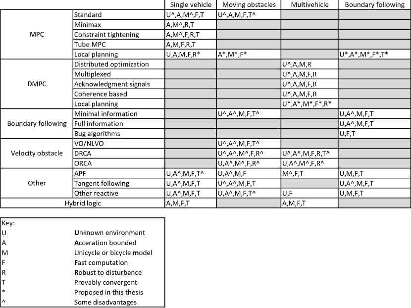
Figure 2.1: Summary of the methods reviewed.

These methods will be discussed in the remainder of this chapter.

2.4 Model Predictive Control

If a obstacle-avoiding trajectory is planned off-line, there are many examples of path following systems which are able to robustly follow it, even if subjected to bounded disturbance. However the lack of flexibility means the environment would have to be perfectly known in advance, which is not conducive to on-line collision avoidance.

Model Predictive Control (MPC), is increasingly being applied to vehicle navigation problems. It is useful as it combines path planning with on-line stability and convergence guarantees, see e.g. [279, 237]. This is basically done by performing the path planning process at every time instant, then applying the initial control related to the chosen trajectory to the vehicle. In most cases a partial path is planned (such that it would not usually arrive at the target), which terminates with an invariant vehicle state. The navigation law would attempt to minimize some ‘cost-to-go’ or navigation function corresponding to the target.

In recent times, MPC has been increasingly being applied to vehicle navigation problems, and it seems to be a natural method for vehicles to navigate. Note discussion of MPC-based approaches applicable to unknown environments is reserved until Sec. 2.5.3.

2.4.1 Robust MPC

The key advantage of MPC lies with its robust variants, which are able to account for set bounded disturbance (and are the most useful for vehicle navigation). These can be categorized into three main categories:

• Min-max MPC. In this formulation, the optimization is performed with respect to all possible evolutions of the disturbance, see e.g. [296]. While it is the optimal solution to linear robust control problems, its high computational cost generally precludes it from being used for vehicle navigation.

• Constraint Tightening MPC. Here the state constraints are dilated by a given margin so that a trajectory can guaranteed to be found, even when disturbance causes the state to evolve towards the constraints imposed by obstacles (see e.g. [277, 278, 172]). The basic argument shows a future viable trajectory exists using a feedback term, through a feedback input is not directly used for updating the trajectory. This is commonly used for vehicle navigation problems – for example a system has been described where an obstacle avoiding trajectory is found based on a minimization of a cost functional compromising the control effort and maneuver time [278]. In this case, convergence to the target and the ability to overcome bounded disturbances can be shown.

• Tube MPC. This uses an independent nominal model of the system, and employs a feedback system to ensure the actual state converges to the nominal state (see e.g. [177]). In contrast, the constraint tightening system would essentially take the nominal state to be the actual state at each time step. This formulation is more conservative than constraint tightening, since it wouldn’t take advantage of favorable disturbance. Thus it doesn’t offer significant benefits for vehicle navigation problems when a linear model is used. However, it is useful for robust nonlinear MPC (see e.g. [236]), and problems where only partial state information is available (see e.g. [295]). Also, the approach proposed in this report, along with any approach which includes path following with bounded deviation (see e.g. [70]), is somewhat equivalent to tube MPC.

For robust MPC, the amount of separation required from the state constraints on an infinite horizon is determined by the Robustly Positively Invariant (RPI) set, which is the set of all possible state deviations that may be introduced by disturbance while a particular disturbance rejection law is operating. Techniques have been developed to efficiently calculate the smallest possible RPI set (the minimal RPI set) [268].

If disturbance is Gaussian rather than set bounded, the MPC vehicle navigation problem may be reformulated stochastically so the overall risk of collision is bounded to an arbitrary level, see e.g. [36, 78]. This may be an interesting area of future research.

2.4.2 Nonlinear MPC

The current approaches to MPC-based vehicle navigation generally rely on linear kinematic models, usually with double integrator dynamics. While many path planning approaches exist for vehicles with nonholonomic kinematics, it is generally harder to show stability and robustness properties [206]. Approaches to robust nonlinear MPC are generally of the tube MPC type [236].

In these cases, a nonlinear trajectory tracking system can be used to ensure the actual state converges to the nominal state. A proposition has been made to also use sliding mode control laws for the auxiliary system [281]. Sliding mode control was employed in this report, and through such systems typically require continuous time analysis, disturbance rejection properties are typically easier to show.

In terms of vehicle navigation problems, examples of MPC which apply unicycle kinematics while having disturbance present have been proposed, see e.g. [70, 69]. However it seems more general applications of nonlinear MPC to vehicle navigation problems should be possible; for example in this report a new control method employing tube MPC principles is proposed.

There are other methods in which MPC may be applied to vehicle navigation problems other than performing rigorously safe path planning. In some cases the focus is shifted towards controlling vehicle dynamics, see e.g. [260, 358, 119]. These use a realistic vehicle model during planning, and are able to give good practical results, through guarantees of safety are currently easier with kinematic models. In other cases MPC may be used to regulate the distance to obstacles, see e.g. [304]. However, this discussion of this type of method is reserved until Sec. 2.5.1.

2.4.3 Planning Algorithms

Global path planning is a relatively well studied research area, and many thorough reviews are available see e.g. [116, 201]. MPC may be implemented with a number of different path planning algorithms. The main relevant measure of algorithm quality is completeness, which indicates whether calculation of a valid path can be guaranteed whenever one exists. Some common global path planning algorithms are summarized:

• Rapidly–Exploring Random Trees. Creates a tree of possible actions to connect initial and goal configurations (see e.g. [72, 149]). Some variants are provably asymptotically optimal [149].

• Graph search algorithms. Examples include A* (see e.g. [283]) and D* (see e.g. [163]). Most methods hybridize the environment into a square graph, with the search calculating the optimal sequence of node transitions. However in many approaches the cells need not be square and uniform, see e.g. [146, 27].

• Optimization of parameterized paths. Examples include Bezier curves [313], splines [182] and polynomial basis functions [265]. While these are inherently smoother, showing completeness may be more difficult in some situations.

• Mathematical programming and optimization. This usually is achieved using Mixed Integer Linear Programming (MILP) constraints to model obstacles as multiple convex polygons [3]. Currently this is commonly used for MPC approaches.

• Tangent Graph based planning. This limits the set of trajectories to cotangents between obstacles and obstacle boundary segments, from which the minimum length path being found in general [289, 332]. The problem of shortest path planning in a known environment for unicycle-like vehicles with a hard constraint on the robot’s angular speed was solved in [289]. It is assumed that the environment consists a number of possibly non-convex obstacles with a constraint on their boundaries curvature and a steady target that should be reached by the robot. It has been proved the shortest (minimal in length) path consists of edges of the so-called tangent graph. Therefore, the problem of the shortest path planning is reduced to a finite search problem.

• Artificial Potential Field Methods. These methods are introduced in Sec. 2.5.2, and are ideally suited to online reactive navigation of vehicles. These can also be used as path planning approachs, essentially by solving the differential equations corresponding to the closed loop system (see e.g. [280]). However, these trajectories would not be optimal and have the same drawbacks as the original method in general.

• Evolutionary Algorithms, Simulated Annealing, Particle Swarm Optimization. These are based on a population of possible trajectories, which follow some update rules until the optimal path is reached (see e.g. [363, 32]). However these approaches seem to be suited to complex constraints, and may have slower convergence for normal path planning problems.

• Partially Observable Markov Decision Processes. This calculates a type of decision tree for different realizations of uncertainty, and uses probabilistic sampling to generate plans that may be used for navigation over long time frames (see e.g. [170]). However this does not seem necessary for MPC-based navigation frameworks.

2.5 Sensor Based Techniques

In comparison to path planning based approaches, sensor based navigation techniques only have limited local knowledge about the obstacle, similar to what would be obtained from range finding sensors, cameras, or optic flow sensors. Reactive schemes are a subset of these which may be interpreted as a mapping between the current sensor state and the actuator outputs; thus approaches employing even limited memory elements would not be considered reactive.

A method for constraint-based task specification has been proposed for sensor-based vehicle systems [68]. This may provide a fixed design process for designing reactive navigation systems (an example of contour tracking is given), and this concept may be an interesting area of future work.

2.5.1 Boundary Following

Boundary following is a direct subproblem of obstacle avoidance, and in most cases a closed loop trajectory bypassing an obstacle can be segmented into ‘boundary following’ and ‘pursuit’ actions, even if this choice is not explicitly deliberated by the navigation law. Boundary following by itself also has many direct uses such as border patrol, terrain tracking and structure monitoring; for application examples see e.g. [114].

Distance Based

In many approaches, boundary following can be rigorously achieved by only measuring the minimum distance to the obstacle, see e.g. [230, 223]. For example, a navigation strategy has been proposed using a feedback controller based on the minimum obstacle distance, and is suitable for guiding nonholonomic vehicles traveling at constant speed [230]. In Chapt. 7 a similar feedback strategy is proposed which only requires the rate of change of the distance to the obstacle as input.

Other approaches have been proposed which use a single obstacle distance measurement at a specific angle relative to the vehicle [330, 224, 328, 327, 158]. These can be classified based on the required measurement inputs; navigation can be based purely on the length of the detection ray [328, 327]; or additionally based on the tangential angle of the obstacle at the detected point [330, 224], or additionally based on estimation of the boundary curvature [158]. Additional information would presumably result in improved behavior, through methods employing boundary curvature may be sensitive to noise, and performance may degrade in such circumstances. Several of these methods are in the realm of switched controllers, for which rigorous theoretical results are available [288, 312]. Unfortunately, impartial comparisons of the closed loop performance of these approaches would be difficult.

Some other methods using similar assumptions are focused on following straight walls, see e.g. [357, 29, 48, 139]. However it seems, at least theoretically, navigation laws capable of tracking contours are more general and therefore superior.

In most these examples the desired behavior can be rigorously shown. However, the common limitation is that the vehicle must travel at constant speed, and this this speed must be set conservatively according on the smallest feature of the obstacle. In some cases simple heuristic can partially solve this problem; by instructing the vehicle to instantly stop and turn in place if the obstacle distance becomes too small, collision may be averted [330].

Sliding Mode Control

Special consideration should be given to sliding mode control based navigation approaches, which are increasingly being applied to vehicle navigation problems where limited sensor information is available, see e.g. [224, 328, 327, 223, 232, 231]. In this context, sliding mode control consists of a discontinuous, switching navigation law which allows rigorous mathematical analysis, and has the additional benefit of having a high resistance to noise, disturbance and model deviation, see e.g. [339]. In the context of collision avoidance, sliding mode control approaches usually are designed as boundary following approaches, through they have also been applied to the avoidance of moving obstacles, and show promising results in that area (see Sec. 2.6.3).

Full Information Based

In situations where more information about the obstacle is available, a clearer view of the immediate environment can be recreated. This means more informed navigation decisions may be able to be made. This can lead to desirable behaviors, such as variable speed and offset distance from the obstacle. It also allows us to loosen some of the assumptions on the obstacle shape and curvature. An example of such behavior may be slowing down at concavities of a boundary and speeding up otherwise, or completely skipping concavities of sufficiently small size that serve only to introduce singularities into the motion. [230, 158].

One such approach using abstract obstacle information is the VisBug class of algorithms, which navigates towards a visible edge of an obstacle inside the detection range (see e.g. [204, 250, 176]). However, these algorithms are concerned with the overall strategy, and are not concerned with details relating to vehicle kinematics or the sensor model. Several approaches have been able to account for the vehicle dynamics, but still have inadequate models of the vehicle sensor. This is similar to the joggers problem, whose solution involves ensuring safe navigation by ensuring the vehicle can stop in the currently sensed obstacle free set [307]. However, an abstract sensor model was used, which presumes the vehicle has continuous knowledge about the obstacle set. A navigation approach which achieves boundary following by picking instant goals based on observable obstacles has been proposed [110]. A ray based sensor model is used, through a velocity controlled holonomic model is assumed. Instant goals have also been used where allowance is made for the vehicle kinematics, however in this case a ray-based obstacle sensor model was not used [111].

In Chapt. 4 a novel MPC-based approach to boundary following is proposed, which generates avoidance constraints and suitable target points to achieve boundary following. This is an interesting, original application of MPC, and may be useful for other types of sensor based navigation problems.

Bug Algorithms

The boundary following navigation laws mentioned previously may perform target-convergent navigation when coupled with high level behavior resembling Bug algorithms (see e.g. [230, 223, 218]). Bug algorithms achieve global convergence by switching between ‘boundary following’ and ‘target pursuit’ modes. By combining these systems, the main additional complexity involves finding and analyzing the conditions for switching between the two modes. While these can be proven to converge to the target, it is important to note pure reactive navigation laws will fundamentally be subjected to local minima problems and will not lead to provable target convergence – this is impossible in general with a reactive, deterministic methods [223]. A number of heuristics exist to prevent these, through they would not be classified as reactive (see e.g. [257]).

2.5.2 Non–Trajectory Based Obstacle Avoidance

In this section, methods which neither explicitly generate a path nor explicitly perform boundary following are described. This includes for example potential field based methods.

Many approaches to this particular problem assume holonomic velocity controlled vehicles. However, this turns out not to be a severe limitation since methods are available for extending these basic navigation laws to account for arbitrary dynamics (including acceleration constraints) are available, see e.g. [240, 243, 37]. This method is based on a coordinate transformation, which effectively provides a zone around the vehicle that contains all perturbations introduced by the dynamics. This method may be applied to a range of navigation approaches, through it may be conservative in some situations. Alternatively a method has been proposed which guarantees collision avoidance simply by ensuring the distance to obstacles is always greater than the stopping distance [210]. Through more conservative, this approach may be useful in cases where little is known about the vehicle model.

Artificial Potential Field Methods

A classic approach to reactive collision avoidance is to construct a virtual potential field that causes repelling from obstacles and attraction to the target. These are termed Artificial Potential Field (APF) methods, and this continues to be an active area of research. Several improvements are listed as follows:

• Unicycle kinematics. Performance can be improved on vehicles with unicycle type kinematics. Specifically, this involves moving the vehicles reference point slightly away from the center of the vehicle, see e.g. [341, 273].

• Local minima avoidance. The shape of the potential field can be designed to flow around obstacle concavities; these are termed harmonic potential fields and provide better performance with local minima, see e.g. [216, 215]. However, it seems impossible to deterministically avoid local minima using reactive algorithms.

• Closed loop performance. Alteration to the shape of the potential field leads to an improvement to the closed loop performance, see e.g. [157, 60]. However in general, the closed loop trajectories of APF based methods would not be optimal. Additionally, reductions of oscillation in narrow corridors may be achieved, see e.g. [272, 273].

• Limited obstacle information. Examples are available where only the nearest obstacle point is available [52]. Several approaches assume global knowledge about the workspace, and thus would not suitable for sensor based navigation.

• Actuator constraints. Examples which focus on satisfying actuator constraints are also available, see e.g. [105, 200].

Tangent Based Methods

Many approaches can be classified as being tangent based, in the sense that they generally only consider motions towards the tangents of obstacles. It has been shown the distance optimal transversal of a cluttered environment can be taken from elements of the tangent graph, which is the set of all tangents between objects, see e.g. [289, 199]. In these cases a method of probabilistically convergent on-line navigation involves randomly choosing tangents to travel down (see e.g. [289]), or by use of the deterministic TangentBug algorithm (see e.g. [147]).

Tangent events can be detected from a ray based sensor model (see e.g. [301]) or by processing data from a camera sensor (see e.g. [140]). This results in an abstract tangent sensor which reports the angle to tangents around the vehicle. A common method of achieving obstacle avoidance is to maintain a fixed angle between the tangent and the vehicles motion, see e.g. [300, 140].

Optic Flow Based Methods

.

This type of navigation is inspired by models of insect flight, where the navigation command is derived from the average rate of pixel flow across a camera sensor (see e.g. [40, 137, 124, 249]). From this rate of pixel flow, a navigation command may be reactively expressed, and good experimental results have been achieved. While this method has the advantage of using a compact sensor and requiring low computational overhead, general mathematical analysis of such navigation laws for showing collision avoidance seems more difficult than the equivalent analysis for range based sensors.

Other Reactive Methods

There are some other variations of approaches which achieve collision avoidance:

• The Safe Maneuvering Zone is suited for kinematic unicycle model with saturation constraints, when the nearest obstacle point is known [179]. This is somewhat similar the Deformable Virtual Zone, where the navigation is based on a function of obstacle detection ray length [180], through collision avoidance is not explicitly proven.

• The Vector Field Histogram directs the vehicle towards sufficiently large gaps between detection rays [337]. The Nearness Diagram is an improved version which employs a number of behaviors for a number of different situations, providing good performance even in particularly cluttered environments (see e.g. [241, 242]).

• A collision avoidance system based on MPC has been proposed and shown to successfully navigate real-world helicopters in unknown environments based on the nearest obstacle point within the visibility radius [304]. However this is less concerned with a proof of collision avoidance, and more with controlling vehicle dynamics.

• A different class of navigation law is based on the Voronoi Diagram, which essentially describes the set of points equidistant from adjacent obstacles. In general it leads to longer paths than the tangent graph, through it represents the smallest set of trajectories which span the free space in an environment. Navigation laws have been developed to equalize the distance to obstacles, when a velocity controlled unicycle kinematic model is assumed (see e.g. [345]).

2.5.3 Sensor Based Trajectory Planning

Trajectory planning using only sensor information was originally termed the joggers problem, since the vehicle must always maintain a path which brings it to a halt within the currently sensor area, see e.g. [307, 12].

The classic Dynamic Window (see e.g. [101, 255, 254]) and Curvature Velocity Method (see e.g. [96, 301]) can be interpreted as a planning algorithm with a prediction horizon of a single time step [255]. To this end, the range of considered control inputs is limited to those bringing the vehicle to a halt within the sensor visibility area, using only circular paths. This can also be easily extended to other vehicle shapes and models [294]. Additionally, measures are available which may reduce oscillatory behavior [318]. A wider range of possible trajectory shapes has also been considered, through it is unclear whether it significantly improves closed loop performance [37]. The Lane-Curvature Method (see e.g. [161]), and the Beam-Curvature Method (see e.g. [96, 301]) are both variants based on a slightly different trajectory selection process. However, in all these cases a similar class of possible trajectories is employed.

In all these cases the justification for collision avoidance is essentially the same argument (the vehicle can stop while moving along the chosen trajectory). The differences in performance are mainly heuristic, and in particular they do not fully account for disturbance and noise. However, an approach similar to the dynamic window was extended to cases where safety constraints must be generated by processing information from a ray-based sensor model [131].

MPC-type approaches have previously been used to navigate vehicles in unknown environments, see e.g. [167, 44, 355]. In most approaches the MPC navigation system is combined with some type of mapping algorithm; however, these often lack the rigorous collision avoidance guarantees normally provided in full-information MPC approaches. In Chapt. 3, a trajectory planning method is proposed, and while it is somewhat similar to the Dynamic Window class of approaches, it implements a control framework somewhat similar to robust MPC. Accordingly, collisions avoidance may be shown even under disturbance.

2.6 Moving Obstacles

Certain types of autonomous vehicle will unavoidably encounter moving obstacles, which are generally more challenging to avoid than static equivalents. The main factors which affect the difficulty of this problem are the characterization of the possible actions another object might take; the increased complexity of the search space and terminal constraints in the case of path planning; and additional conservativeness in the case of sensor based systems.

At one extreme, an obstacle translating at constant speed and in a constant direction may be accounted for by merely considering the future position of the obstacle. The other extreme is an obstacle pursuing the vehicle, for which the set of potential locations grows polynomially along the planning horizon. Several offerings also describe integrated approaches, including obstacle motion estimation from LiDAR sensors [246]. However in this section discussion is focused on the avoidance behavior.

General planning algorithms suited for dynamic environments are also available, however in the absence of obstacle assumptions it is impossible to guarantee existence of a viable path, see e.g. [112]. When planning in known environments, states which necessarily lead to collision – the Inevitable Collision States (ICS) – may also be abstracted and used to assist planning [263]. If the motion of vehicles is known stochastically, the overall probability of collision for a probational trajectory may also be computed based on the expected behavior of other obstacles, see e.g. [11].

2.6.1 Human–Like Obstacles

Several works attempt to characterize the motion of moving obstacles. For avoiding humans, several models of socially acceptable pedestrian behavior are available (see e.g. [310, 256, 100, 367]). An approach which avoids obstacles based on the concept of personal space has been proposed and works well in practice [256]. Other approaches can avoid human-like obstacles while also considering the reciprocal effect of the vehicles motion have also been proposed [100, 367].

2.6.2 Known Obstacles

Obstacles translating at constant speed and in a constant direction may be avoided using the concept of a velocity obstacle, see e.g. [303, 97, 98]. This is essentially the set of vehicle velocities that will result in collision with the obstacle, and by avoiding these velocities, collisions may be avoided. This result may be extended to arbitrary (but known) obstacle paths and more complex vehicle kinematics using the nonlinear velocity obstacle, see e.g. [181]. The velocity obstacle method also extends to 3D spaces, see e.g. [305, 356].

2.6.3 Kinematically Constrained Obstacles

When obstacles are only known to satisfy nominal kinematic constraints, the set of possible obstacle positions grows over time. Avoidance may be ensured by either trajectory based methods or reactive methods.

Trajectory Based Methods

There are three basic methods of planning trajectories which avoid such obstacles:

• Ensuring that whenever a collision could possibly occur the vehicle is stationary – this is referred to as passive motion safety (see e.g. [42, 25]). In some situations it is impossible to show any higher form of collision avoidance, through it ultimately relies on the behavior of obstacles to avoid collisions.

• Ensuring the vehicle can move arbitrarily far away from the obstacle over a infinite horizon. In one such approach the the time-minimal paths to achieve a particular task were calculated [343]. Similar examples of approaches include more allowance for other uncertainties, see e.g. [78].

• Ensuring the vehicle lies in a set of points that cannot be easily reached by the obstacle [353]. Under certain assumptions a non-empty set of points may be found which lies just behind the obstacles velocity vector. This allows avoidance over a infinite horizon, while being possibly less conservative than the previous option.

When performing path planing in a sensor based paradigm, the same types of approaches may be used, through collision avoidance may be harder to show for general obstacle assumptions. The main additional assumption is that any occluded part of the workspace must be considered as a potential dynamic obstacle [59, 42]. Naturally this makes the motion of any vehicles even more conservative.

Reactive Methods

When moving obstacles are present in the workspace, it is still possible to design reactive navigation strategies which can provably prevent collisions, at least with some more restrictive assumptions about the obstacles motion. These methods are outlined as follows:

• When obstacle are sufficiently spaced (so that multiple obstacles must not be simultaneously avoided), an extension of the velocity obstacle method has been designed to prevent collisions [349, 293]. This effectively steers the vehicle towards the projected edge of the obstacle, and was applied to the semi-autonomous collision avoidance of robotic wheelchairs.

• Certain boundary following techniques proposed in Sec. 2.5.1 have been successfully extended to moving obstacles and maintain provable collision avoidance, assuming the obstacles are sufficiently spaced and their motion and deformation is known to satisfy some smoothness constraints, see e.g. [292, 234]. These are all based on sliding mode control, which retains the advantages discussed previously in Sec. 2.5.1.

• Some artificial potential field methods have been extended to moving obstacles, through rigorous justification is not provided (see e.g. [273, 109]).

2.7 Multiple Vehicle Navigation

Navigation of multiple vehicle systems has gained much interest in recent years. As autonomous vehicles are used in greater concentrations, the probability of multiple vehicle encounters correspondingly increases, and new methods are required to avoid collision.

The study of decentralized control laws for groups of mobile autonomous robots has emerged as a challenging new research area in recent years (see, e.g., [285, 346, 228, 261, 227] and references therein). Broadly speaking, this problem falls within the domain of decentralized control, but the unique aspect of it is that groups of mobile robots are dynamically decoupled, meaning that the motion of one robot does not directly affect that of the others. This type of systems is viewed as a networked control system, which is an active field of research. For examples of more generalized work in this area, see e.g. [226, 286, 287, 229]. One of the important applications of navigation of multi-vehicle systems is is in sensing coverage. To improve coverage and reduce the cost of deployment in a geographically vast area, employing a network of mobile sensors for the coverage is an attractive option. Three types of coverage problems for robotic were studied in recent years; blanket coverage [290], barrier coverage [54, 55], and sweep coverage [54, 56]. Combining existing coverage algorithms with effective collision avoidance methods in an open practically important problem.

While there is an extensive literature on centralized navigation of multiple vehicles, it is only briefly mentioned here, since it is generally not applicable to arbitrarily scalable on-line collision avoidance systems. Examples of off-line path planning systems which can find near optimal trajectories for a set of vehicles are available, see e.g. [313]. Another variation of this problem involves a precomputed prescription of the paths to be followed, where the navigation law must only find an appropriate velocity profile which avoids collisions (see e.g. [262, 65]).

2.7.1 Communication Types

There are three common modes of communication in multiple vehicle collision avoidance systems:

• Direct state measurement. This can be achieved using only sensor information to measure the state of the surrounding vehicles, and is used in many non-path based reactive approaches.

• Single direction broadcasting. In addition to the physical state of the vehicle, additional variables are also transmitted, usually relating to the current trajectory of the vehicle. As discussed in Chapt. 5, this allows the projected states of other vehicles to be avoided during planning. This type of communication is occasionally referred to as sign board based.

• Two way communication. This can range from simple acknowledgment signals to full decentralized optimization algorithms. These are commonly used for decentralized MPC, though some MPC variants have been proposed where sign boards are sufficient.

A number of different models of communication delay and error are considered in networked navigation problems. The ability to cope with unit communication delays, packet dropouts and finite communication ranges is definitely desirable in any navigation system.

2.7.2 Reactive Methods

The most basic from of this problem only considers a small number of vehicles. For example, navigation laws have been proposed to avoid collisions between two vehicles traveling at constant speed with turning rate constraints, see e.g. [102, 326]. A common example of this type of system is an Air Traffic Controller (ATC). However, these types of navigation systems do not directly relate to avoiding collisions in cluttered environments [169].

Potential Field Methods

Potential field methods may be constructed to mutually repel other vehicles. In some ways this approach is more satisfactory than the equivalent methods applies to static obstacles – for example local minima are less of an issue in the absence of contorted obstacle shapes. Methods have been proposed which avoid collision between a unlimited number of velocity controlled unicycles or velocity controlled linear vehicles [217, 129, 320]. One variant, termed the multi-vehicle navigation function, is able to show convergence to targets in the absence of obstacles. However these still use similar types of repulsive and attractive fields, see e.g. [351, 75, 325].

Other variants also include measures to provably maintainable cohesion between groups, see e.g. [74], while others have also been applied to vehicles with limited sensing capabilities [73]. Many methods provide good results while neglecting mathematical analysis of collision avoidance, see e.g. [52, 85, 88].

In cases where finite acceleration bounds are present (but still without any nonholonomic constraints), an mutual repulsion based navigation system with a more sophisticated avoidance function has been proven to avoid collisions for up to three vehicles [130]. When more vehicles are present, it is possible to back-step the additional dynamics into a velocity controlled model, through this does not lead to bounds on the control inputs of the dynamic model [200].

Many of these methods can be extended to static obstacles, and these combined systems are achieved by the same avoidance functions as the single vehicle case, see e.g. [200]. An interesting question may be whether transformation based approaches allowing arbitrary dynamics (see e.g. [240, 243, 37]) may be extended to multiple vehicle cases. As such, showing collision avoidance for an unlimited number of acceleration constrained vehicles using a repulsive function seems to be an unsolved problem in robotics.

Reciprocal Collision Avoidance Methods

Approaches termed Optimal Reciprocal Collision Avoidance (ORCA) achieve collision avoidance by assuming each vehicle takes half the responsibility for each pairwise conflict, with the resulting constraints forming a set of viable velocities from which a selection can be made using linear programming, see e.g. [342, 315]. Some interesting extensions have been proposed to the RCA concept, for example it has been applied to both nonholonomic vehicles and linear vehicles with acceleration constraints, while maintaining collision avoidance [314, 344, 315]. The method may be extended to arbitrary vehicle models, as rigorous avoidance is achieved though the addition of a generic bounded-deviation path tracking system [269, 315, 10]. These methods are also able to integrate collision avoidance of static obstacles, which easily integrates into the navigation framework.

RCA is an extension of an similar method based on collision cones called Implicit Cooperation [1]. Another method has also been proposed which is based on collision cones, called Distributed Reactive Collision Avoidance (DRCA). This has the benefit of showing achievement of the vehicles objective in limited situations, ensuring minimum speed constraints are met when global information is available, and showing robustness to disturbance [174, 173].

Hybrid Logic Methods

For these approaches, discrete logic rules are used to coordinate vehicles. In most cases, this is achieved through segregation of the workspace into cells, which can each only hold one vehicle, see e.g. [26, 113, 276, 251]. In these cases, collisions can be prevented by devising a scheme where two vehicles do not attempt to occupy the same cell simultaneously. Additionally, many methods of integrating this with control of the vehicle’s dynamics has been proposed, see e.g. [64]. Hybrid control systems are becoming increasingly used to control real world systems (see e.g. [225]).

In some approaches the generation of cells may be on-line and ad-hoc. This is useful when minimum speed constraints are present – the vehicles may be instructed to maintain a circular holding pattern, and then to shift their holding pattern appropriately when safe. In this case some different possibilities for the shifting logic have been proposed, for example based on vehicle priority [168], or traffic rules [259].

2.7.3 Decentralized MPC

While optimal centralized MPC is theoretically able to coordinate groups of vehicles, the underlying optimization process is too complex for any scalable real time application. Examples of centralized MPC for multiple vehicle systems are available (see e.g. [94]).

Decentralized variants of MPC in general do not specifically address the problem of deadlock. For example in [171] a distributed navigation system is proposed which is able to plan near optimal solutions that robustly prevent collisions and allow altruistic behavior between the vehicles which monotonically decrease the global cost function. However this does not equate to deadlock avoidance, which is discussed in Sec. 2.7.4.

A review of general decentralized MPC methods is available [28], along with a review specific to vehicle navigation [306]. There are currently four main methods of generating deconflicted trajectories which seem suitable for coordination of multiple vehicles:

• Decentralized optimization can find the near-optimal solution for a multi-agent system using dual decomposition to find a set of trajectories for the system of vehicles, see e.g. [266, 347, 322]. While this is more efficient than centralized optimization, it requires many iterations of communication exchange between vehicles in order to converge to a solution. Other types decentralized planning algorithms may also be effective, for example a decentralized RRT approach has been proposed which implements the same type of processes [71].

• Other approaches have been proposed using multiplexed MPC (see e.g. [172, 311]), and sequential decentralization (see e.g. [4]). The robust control input for each vehicle may be computed by updating the trajectory for each vehicle sequentially, at least when they are close. While multiplexed MPC is suited to real time implementation, a possible disadvantage is path planning cannot occur simultaneously in two adjacent vehicles. However, the same framework been extended to provide collision avoidance in vehicle formation problems [350].

• Another possible solution is to require acknowledgment signals before implementing a possible trajectory, and has the benefit of not requiring vehicles to be synchronized. This method seems an effective solution [24, 23], however interaction between vehicles may cause planning delays under certain conditions.

• Approaches also have been proposed which permit single communication exchanges per control update [340, 69]. This is done by including a coherence objective to prevent the vehicles from changing its planned trajectory significantly after transmitting it to other vehicles. In Chapt. 5, an original set of trajectory constraints are proposed, which are possibly more general in that they do not explicitly enforce coherency objectives or limit the magnitude of trajectory alterations.

MPC may also easily include maintenance of objectives other than collision avoidance. For example, radio propagation models have been included in the path evaluation function, so that communication between vehicles is maintained [123, 122].

2.7.4 Deadlock Avoidance

The collision avoidance techniques described in the Sec. 2.7.3 will not generally guarantee that vehicles arrive at their required destination. System states which do not evolve to their targets are referred to as deadlocks. Naturally some control laws are more prone to deadlocks than others; this may be investigated using probabilistic verification [258].

It can be shown that when using suitable controllers, multiple vehicles may converge to their targets in open areas, see e.g. [331, 325]. This means a more interesting question relates to deadlock avoidance in unknown, cluttered environments. It seems a generalized solution to the latter would be relatively sophisticated, and require significant overlap with other areas such as distributed estimation, mapping, decision making and control.

Currently, deadlock resolution systems are almost exclusively constructed based on transitions between nodes on a graph or equivalent, and the solution can be described as a resource allocation problem. Variations of this problem comprise a well studied field, see e.g. [207, 113, 142, 275, 276]. A common simple example of such an algorithm is the bankers algorithm, which is based on the concept of only allowing an action to be taken if it leaves appropriate spatial resources so that every other agent may eventually run to completion [156].

However, these types of deadlock avoidance system are somewhat decoupled from the actual sensor information available to the vehicle, and in some cases it would be advantageous to eliminate the need for graph generation and use algorithms that correspond directly to the continuous state space. These algorithms are also generally global solutions, requiring knowledge of the parameters of all other vehicles. In some cases it could be more useful to use a more local approach, especially when there is a very low density of vehicles operating in the environment.

In Chapt. 6 an initial solution to a simplified version of this problem is offered, where only two vehicles are present. In future work it is hoped this can be extended to more general situations.

2.8 Summary

This chapter provides a review of a range of techniques related to the navigation of autonomous vehicles through cluttered environments, which can rigorously achieve collision avoidance for some given assumptions about the system. This continues to be an active area of research, and a number of channels where current approaches may be improved are highlighted. Approaches to avoiding collisions between multiple vehicles along with moving obstacles are considered. In particular, approaches based on local sensor information are emphasized, which seems more difficult and relevant than global approaches where full knowledge of the environment is assumed. Finally, the virtues of recently proposed MPC, decentralized MPC, and sliding mode control based approaches are highlighted, when compared to existing methods.

Chapter 3 Collision Avoidance of a Single Vehicle

In this chapter, the problem of preventing collisions between a vehicle and a set of static obstacles while navigating towards a target position is considered. In this chapter, the vehicle is presumed to have some information about the obstacle set; a full characterization is considered in Chapt. 4. The aim of this chapter is to establish the navigation framework used in all subsequent chapters. Both holonomic and unicycle kinematic motion models are considered (these were informally described in Chapt. 2).

The body of this chapter is organized as follows. In Sec. 3.1, the problem statement is explicitly defined, and the vehicle model is given. In Sec. 3.2, the navigation system structure is presented. Sec. 3.3 offers simulated results. Finally, Sec. 3.4 offers brief conclusions.

3.1 Problem Statement

A single autonomous vehicle traveling in a plane is considered, which is associated with a steady point target $T$. The plane contains a set of unknown, untransversable, static, and closed obstacles $D_{j}\not\ni T,j\in[1:n]$. The objective is to design a navigation law that drives every vehicle towards the assigned target through the obstacle-free part of the plane $F:=\mathbb{R}^{2}\setminus D$, where $D:=D_{1}\cup\ldots\cup D_{n}$. Moreover, the distance from the vehicle to every obstacle and other vehicles should constantly exceed the given safety margin $d_{sfe}$, which would naturally exceed the vehicle’s physical radius.

3.1.1 Holonomic Motion Model

Holonomic dynamics are generally encountered on helicopters and omni-directional wheeled robots. A discrete-time point-mass model of vehicle is used, where for simplicity the time-step $\Delta t$ is normalized to unity and the acceleration capability of the vehicle is assumed to be identical in all directions:

$$\boldsymbol{s}(k+1)=\boldsymbol{s}(k)+\boldsymbol{v}(k)+\frac{1}{2}\cdot\left(\boldsymbol{u}(k)+\boldsymbol{w}(k)\right),$$ (3.1a)

$$\boldsymbol{v}(k+1)=\boldsymbol{v}(k)+\boldsymbol{u}(k)+\boldsymbol{w}(k),$$ (3.1b)

$$v(k):=\lVert\boldsymbol{v}(k)\rVert\leq v_{max},\quad\lVert\boldsymbol{u}(k)\rVert\leq u_{max},\quad\lVert\boldsymbol{w}(k)\rVert\leq w_{max}.$$ (3.1c)

Here $k\in\mathbb{N}$ is the time index; $\boldsymbol{s}=\,\mbox{\bf col}\,(s_{x},s_{y})$ is the vector of the vehicle’s coordinates; $\boldsymbol{v}=\,\mbox{\bf col}\,(v_{x},v_{y})$ is its velocity vector; $\boldsymbol{u}=\,\mbox{\bf col}\,(u_{x},u_{y})$ is the control input; and the disturbance $\boldsymbol{w}=\,\mbox{\bf col}\,(w_{x},w_{y})$ accounts for any kind of discrepancy between the real dynamics and their nominal model. In particular, $\boldsymbol{w}$ may comprise the effects caused by nonlinear characteristics of a real vehicle. Furthermore, $v_{max}$ is the maximal achievable speed; $u_{max}$ is the maximal controllable acceleration; and $w_{max}$ is an upper bound on the disturbance. Only the trajectories satisfying all constraints from Eq.(3.1) are feasible. The state can be abstracted as $\mathscr{S}:=\langle\boldsymbol{s},\boldsymbol{v}\rangle$, and the control input as $\mathscr{U}\equiv\boldsymbol{u}$. The nominal trajectories, generated during planning, are created by setting $\boldsymbol{w}\equiv 0$ (and thus may deviate from the actual ones). Here and throughout, $\lVert\cdot\rVert$ is the standard Euclidean norm.

3.1.2 Unicycle Motion Model

Unicycle motion models describe vehicles which are associated with some heading which determines the direction of movement, with changes to the heading limited by a turning rate constraint. A continuous-time point-mass model of the vehicle with discrete control updates is considered. As before, the time step $\Delta t$ is normalized to unity.

For $k<t\leq(k+1)$:

$$\boldsymbol{s}(t)=\boldsymbol{s}(k)+\int_{k}^{t}\left[\begin{array}[]{c}\cos(\theta(\acute{t})+\varphi(\acute{t}))\\ \sin(\theta(\acute{t})+\varphi(\acute{t}))\\ \end{array}\right]\cdot v(t)d\acute{t}$$ (3.2c)

$$v(t)=v(k)+u_{v}(k)\cdot(t-k)+\int_{k}^{t}w_{v}(\acute{t})d\acute{t},\quad|u_{v}(k)|\leq u_{v,max}$$ (3.2d)

$$\theta(t)=\theta(k)+u_{\theta}(k)\cdot(t-k)+\int_{k}^{t}w_{\theta}(\acute{t})v(\acute{t})d\acute{t},\quad|u_{\theta}(k)|\leq u_{\theta,max}$$ (3.2e)

$$0\leq v(t)\leq v_{max},\quad\lvert\varphi\rvert\leq\varphi_{max},\quad\lvert w_{\theta}\rvert\leq w_{\theta,max},\quad\lvert w_{v}\rvert\leq w_{v,max}$$ (3.2f)

Here $k\in\mathbb{N}$ is the time index; $\boldsymbol{s}=\,\mbox{\bf col}\,(s_{x},s_{y})$ is the vector of the vehicle’s coordinates; $v$ is the scalar speed; $\theta$ is orientation angle; $v_{max}$ is the maximal achievable speed; $\varphi$ is the angular difference between the vehicle orientation and the velocity direction caused by the wheels slip; $w_{\theta}$ is the coefficient of the rotation rate bias due to disturbance; and $w_{v}$ is the longitudinal acceleration bias due to disturbance. This assumes that the maximal feasible rotation rate bias due to disturbance is proportional to the vehicle speed. The state can be abstracted as $\mathscr{S}:=\langle\boldsymbol{s},v,\theta\rangle$, and the control input as $\mathscr{U}:=\langle u_{v},u_{\theta}\rangle$. The nominal trajectories which are generated during planning are created by setting $\varphi\equiv w_{\theta}\equiv w_{v}\equiv 0$, and naturally will deviate from the actual ones.

3.1.3 Sensor Requirements

In this chapter, is is assumed that there is an arbitrary, time varying sensed area $F_{vis}(k)\subset F$ corresponding to a subset of the obstacle free part of the plane. Normally, this would incorporate line-of-slight constraints together with visibility range constraints, which are nominally taken to be $R_{nom}>0$ for the purposes of designing the trajectory planning algorithm (this does not affect robustness properties). At time $k$, it is assumed that for any point $x$, the vehicle has knowledge of the distance to $\mathbb{R}^{2}\setminus F_{vis}(k)$:

$$\text{\bf dist}_{F_{vis}(k)}[x]:=\min_{y\in\mathbb{R}^{2}\setminus F_{vis}}\lVert x-y\rVert$$ (3.3)

At time $k$, it is assumed that the vehicle has knowledge of its state $\mathscr{S}$. It is also assumed that the vehicle has knowledge of the position of the target $T$. Allowing for state measurement noise remains an area of future research, through it seems likely it can be incorporated into the same robust navigation framework proposed here.

3.2 Navigation System Architecture

Model Predictive Control (MPC) is based on iterative, finite horizon optimization of a trajectory corresponding to a given plant model. Chosen over a relatively short time horizon $\tau$ into the future, a probational trajectory, commencing at the current system state $\mathscr{S}$, is found over the horizon $[k,k+\tau]$ at every time instant $k$. When disturbance is absent (considered in Chapts. 4 and 6), the control representing the first time-step is implemented on the vehicle. When disturbance is present (considered in this chapter and Chapt. 5), an auxiliary trajectory tracking controller updates the control to correct deviations from the probational trajectory (this is a somewhat similar concept to the tube MPC methodology). In both cases, at each subsequent time-step, the trajectory planning process is repeated for the new vehicle state and obstacle observations.

Unlike general trajectory planning approaches usually employed by full-information MPC approaches, the planning system only considers a certain subset of possible trajectories. This is a similar concept to the Dynamic Window and Curvature-Velocity methods (see Chapt. 2). This means the simplified trajectory generation scheme proposed in Sec. 3.2.3 is not complete – to accommodate this, if a trajectory cannot be found, the trajectory from the previous time-step is reused, with an appropriate time-shift.

The upper index $(\cdot)^{*}$ is used to mark probational trajectories, and the associated variables depend on two arguments $(j|k)$, where $k$ is the time instant when this trajectory is generated and $j\geq 0$ is the number of time steps into the future (the related value concerns the state at time $k+j$).

3.2.1 Overview

The navigation system consists of two modules; the Trajectory Planning Module (TPM), and the Trajectory Tracking Module (TTM). The TPM may be summarized by sequential execution of the following steps:

1. Generation of a finite set $\mathscr{P}$ of planned trajectories, each starting at the current vehicle state $\mathscr{S}$ (see Sec. 3.2.3).

2. Refinement of $\mathscr{P}$ to only feasible trajectories (see Sec. 3.2.2).

3. Selection of a trajectory from $\mathscr{P}$:

   • If $\mathscr{P}$ is empty, the probational trajectory is inherited from the previous time step (with a proper time shift).

   • Otherwise, the probational trajectory is updated by choosing an element of $\mathscr{P}$ minimizing some cost function (see Sec. 5.2.4).

4. Application of the first control $\mathscr{U}^{*}(0|k)$ related to the selected probational trajectory to the vehicle.

5. $k:=k+1$ and go to S.1.

The TTM runs concurrently to the TPM and updates the vehicle’s control $\mathscr{U}$ (in navigation problems where disturbance is present). The TTM architecture depends on the vehicle model type:

• Holonomic: In this case, TTM updates occur at the same rate as TPM updates, and the TTM may be simply added as an additional step after S.3. This means whenever the probational trajectory is updated rather than inherited, the implemented control will be identical to $\mathscr{U}^{*}(0|k)$.

• Unicycle: In this case, TTM updates occur at a much faster rate than TPM updates; this is because the TTM is implemented as a sliding mode control law (see Sec. 3.2.4). Thus even when a trajectory is updated rather than inherited, the implemented control $\mathscr{U}(t)$ could only be equal to $\mathscr{U}^{*}(0|k)$ only at exact, integral time instants.

3.2.2 Safety Margins

To ensure collision avoidance, TPM respects more conservative safety margins than $d_{sfe}$. They take into account deviations from the probational trajectory caused by disturbances and are based on estimation of these mismatches.

The first such estimate addresses the performance of TTM; let $d_{trk}$ be defined as an upper bound on the translational deviation over the planning horizon between the probational trajectory and the real motion of the vehicle driven by the TPM along this trajectory in the face of disturbances.

Computation of $d_{trk}$ takes into account the particular design of TPM and is discussed in Sec. 3.2.4. To decouple designs of TPM and TTM, the control capacity is a priory distributed between TPM and TTM. Specifically, TPM must generate the controls only within the reduced bounds determined by:

Holonomic:

$$u_{nom}:=\mu\cdot u_{max}$$ (3.4b)

Unicycle:

$$u_{v,nom}:=\mu_{u}\cdot u_{v,max},\quad u_{\theta,max}:=\mu_{\theta}\cdot u_{\theta,max},\quad v_{nom}:=\mu_{v}\cdot v_{max}$$ (3.4c)

The remaining control capacity is allotted to TTM. Here $\mu$, $\mu_{u}$, $\mu_{\theta}$, $\mu_{v}\in(0,1)$ are tunable design parameters.

Additionally, for unicycle vehicles, one additional constraint on the absolute curvature of the path is present – the curvature must fall below a level accessible by the vehicle. Since this level depends on the actual speed $v(t)$, which is influenced by unknown disturbances, it is required that the curvature of the planned path must fit the worst case scenario. In other words, it should not exceed:

$$\varkappa_{max}:=\frac{u_{\theta,max}}{v_{max}}.$$ (3.5)

In fact, a tighter bound is required – the curvature should not exceed $\varkappa_{nom}:=\mu_{\varkappa}\cdot\varkappa_{max}$. Here $\mu_{\varkappa}\in(0,1)$ is a design parameter chosen similarly to those in Eq.(3.4).

Along with the system parameters, the control capability allotments $\mu$, $\mu_{u}$, $\mu_{\theta}$, $\mu_{v}$, $\mu_{\varkappa}$ uniquely determine the estimate $d_{trk}$ (for the adopted design of TPM), as will be shown in Sec. 3.2.4. In particular, it should be noted $d_{trk}$ does not depend on the choice of the probational trajectory.

The following more conservative safety margins account for not only disturbances but also the use of time sampling in measurements of relative distances:

$$d_{tar}:=d_{sfe}+\frac{v_{max}}{2}+d_{trk}$$ (3.6)

To illuminate their role, the following definition is introduced:

Definition 3.2.1

A probational trajectory is said to be feasible if the distance from any way-point to any static obstacle exceeds $d_{tar}$ for any trajectory.

The motivation behind this definition is illuminated by the following:

Lemma 3.2.1

Let the probational trajectory adopted for use at time step $k-1$ be feasible. Then despite of the external disturbances, the vehicles do not collide with obstacles on time interval $[k-1,k]$, and also respect the required safety margin $d_{sfe}$.

Proof

For any $t\in[k-1,k]$, it is known vehicle deviates from the related position on the probational trajectory by no more than $d_{trk}$. Consider the end $k_{\ast}$ of the interval $[k-1,k]$ nearest to $t$; the times $t$ and $k_{\ast}$ are separated by no more than half time-step. So thanks to the upper bound on the speed, the nominal positions at times $t$ and $k_{\ast}$ differ by no more than $\frac{v_{max}}{2}$. Overall, the distance between the way-point on the probational trajectory that is related to time step $k_{\ast}$ and the actual position at time $t$ does not exceed $\frac{v_{max}}{2}+d_{trk}$. Since the distance from this way-point to any static obstacle exceeds $d_{tar}$, the distance from the real position at time $t$ is no less than $d_{tar}-\frac{v_{max}}{2}-d_{trk}=d_{sfe}$. $\quad\bullet$

Remark 3.2.1

For arbitrary (not unit) sampling time $\Delta t$, the addend $\frac{v_{max}}{2}$ in Eq.(3.6) should be replaced by $\frac{v_{max}}{2}\Delta t$. This addend asymptotically vanishes as $\Delta t\to 0$; so typically $d_{trk}$ would too provided that the discrete planning horizon $\tau$ is upper bounded. Thus the conservatism imposed by the extra addends in Eq.(3.6) may be attenuated by reducing the time step employed during the planning process. As the time-step is conversely increased, $d_{trk}$ grows but remains bounded even if $\Delta t\to\infty$, as will be discussed in Sec. 3.2.4. However the other addend $\frac{v_{max}}{2}\Delta t$ grows without limits as $\Delta t\to\infty$.

Overly enhanced margins Eq.(3.6) may make the navigation objective unachievable; for example, the corridors amidst the obstacles may be too narrow to accommodate a distance of no less than $d_{tar}$ to the both sides of the corridor. In fact, feasibility of the enhanced margins is the basic requirement regulating the practical choice of $\Delta t$. In the case of heavy uncertainty about the scene, a reasonable option is to pick $\Delta t$ so that the quantization error $\frac{v_{max}}{2}\Delta t$ is comparable with the limit bound on the disturbance-induced error $d_{trk}$.

3.2.3 Trajectory Planning

Trajectory generation could potentially use many forms, and some varieties of commonly used approaches were outlined in Chapt. 2. However in the approach proposed here, a simplified version is designed for the following reasons:

• Compared to commonly used optimization approaches, the proposed method is able to improve tractability while not significantly influencing closed loop performance. Similar types of simplified planning methods have been proposed previously, see e.g. [255, 37].

• In Chapt. 5 it will be possible to make certain inferences about the possible trajectories of other vehicles.

Here two tunable parameters are used; $\Delta v$ and $\Delta\Lambda$, which determine the ‘mesh’ size for trajectory generation.

Longitudinal Control Pattern

The generated set of trajectories $\mathscr{P}$ consists of two parts $\mathscr{P}_{+}$ (cruising trajectories) and $\mathscr{P}_{-}$ (slowing trajectories), with each part being composed of trajectories matching a given pattern of speed evolution over the planning horizon:

• The pattern $p_{+}:=(+--\ldots)$ means that the initial speed $v^{\ast}(0|k):=v(k)$ is first increased by a given tunable speed increment $\Delta v$:

  Holonomic:

  $$v_{+}^{\ast}(1|k)=\min\big{\{}v^{\ast}(0|k)+\Delta v;v_{max}\big{\}},\quad\Delta v<u_{nom}\times(1\,\text{time unit})\equiv u_{nom}\Delta t$$ (3.7b)

  Unicycle:

  $$v_{+}^{\ast}(1|k)=\min\big{\{}v^{\ast}(0|k)+\Delta v;v_{nom}\big{\}},\quad\Delta v<u_{v,nom}\times(1\,\text{time unit})\equiv u_{v,nom}\Delta t$$ (3.7c)

  The speed bounds follow from Eq.(3.4). The associated control inputs which achieve this pattern is given in Sec. 3.2.3. The planned speed is then constantly decreased by subtracting $\Delta v$ at all subsequent time steps $j\geq 1$ (while preventing the speed from taking a meaningless negative value):

  $$v_{+}^{\ast}(j+1|k)=\max\big{\{}v^{\ast}(j|k)-\Delta v,0\big{\}}$$ (3.8)

• The pattern $p_{-}=(---\ldots)$ means the speed is constantly decreased in accordance with Eq.(3.8), creating a second speed profile $v_{-}^{\ast}(j|k)$.

The feasibility of this control pattern is illustrated in Fig. 3.1. The planning horizon $\tau$ is selected from the requirement that when following any generated trajectory, the vehicle halts within this horizon:

$$\tau:=\begin{cases}\tau_{-}=\left\lceil\frac{{v(k)}}{{\Delta v}}\right\rceil&\text{for slowing trajectories}\\[5.0pt] \tau_{+}=\left\lceil\frac{{v(k)}}{{\Delta v}}\right\rceil+2&\text{for cruising trajectories},\end{cases}$$ (3.9)

where $\left\lceil a\right\rceil$ is the integer ceiling of the real number $a$. This horizon is determined by the current vehicle speed $v(k)$ and may vary over time, though it may also be fixed so it is equal to an upper bound of all possible values. To ensure obstacle avoidance, attention is limited to trajectories for which the vehicle halts within the planning time horizon and observed part of the environment.

Remark 3.2.2

The length of any planned trajectory does not exceed $l=v_{max}+\frac{v_{max}^{2}}{2\cdot u_{v,nom}}$. It seems prudent to adjust relevant parameters so the trajectory remains within the sensed area, so it follows that $(l+d_{tar})$ is less than the nominal sensor range $R_{nom}$.

From this point, the subscript $(\cdot)_{\pm}$ is used to annotate variables which may correspond to either speed profile $p_{+}$ or $p_{-}$.

Lateral Control Pattern

The lateral profile of the trajectories is constrained to invariably consist of a sharp turn, followed by a reduced turn, followed by a straight section.

Holonomic

To formulate this, first consider how the angle of the vehicle’s velocity vector changes over each time step. Starting from an initial angle $\theta(0|k)$ given by the vehicle actual velocity vector $\boldsymbol{v}(k)$, the progression $\theta(j|k)$ is bounded by:

$$\lvert\underbrace{\theta(j+1|k)-\theta(j|k)}_{\Delta\theta(j|k)}\rvert\leq\Delta\theta_{\max}(j|k).$$ (3.10)

If $\boldsymbol{v}(k)\equiv 0$, $\theta(0|k)$ is arbitrary. If $\theta^{*}(j|k)$ is known, the velocity vector, and thus the vehicle position vector, may be trivially found over the length of the trajectory by evaluating Eq.(3.1).

The maximal angular deviation $\Delta\theta_{\max}(j|k)$ between the vectors $\boldsymbol{v}^{\ast}(j+1|k)$ and $\boldsymbol{v}^{\ast}(j|k)$ is determined by the speed profile $v_{\pm}^{*}(j|k)$ and constant $u_{nom}$. Specifically, $\Delta\theta_{\max}(j|k)=\pi$ if $v_{\pm}^{*}(j|k)+v_{\pm}^{*}(j+1|k)\leq u_{nom}$; otherwise Fig. 3.1 and the well-known formula giving the angle of a triangle with three known sides imply that:

$$\Delta\theta_{\max}(j|k)=\arccos\frac{v_{\pm}^{*}(j|k)^{2}+v_{\pm}^{*}(j+1|k)^{2}-u_{nom}^{2}}{2v_{\pm}^{*}(j+1|k)v_{\pm}^{*}(j|k)}.$$ (3.11)

Figure 3.1: The set of possible values of the next probational velocity.

In this formulation, the overall turning profile can be uniquely described by a scalar $\Lambda(k)$. Small values correspond to short turns, while large values correspond to long turns:

$$\Delta\theta(j|k)=\Delta\theta_{\max}(j|k)\cdot\text{\bf sgn}(\Lambda(k))\cdot\text{\bf sat}_{0}^{1}(\lvert\Lambda(k)\rvert-j).$$ (3.12)

Here the function $\text{\bf sat}_{b}^{a}(x):=\min\{\max\{x,b\},a\}$, and the function $\text{\bf sgn}(\cdot)$ is the standard signum function. The possible values of $\Lambda$ considered here are discretized by an integer $m$, and are given by:

$$\Lambda(k)=m\cdot\Delta\Lambda,\quad\left\{m\in\mathbb{I}:\lvert m\rvert<\left\lceil\frac{\tau}{\Delta\Lambda}\right\rceil\right\}$$ (3.13)

For each $m$, a planned trajectory may be uniquely determined using the nominal equations Eq.(3.1), along the initial state $\mathscr{S}(k)$, and the speed profile $p\in\{p_{+};p_{-}\}$.

Unicycle

The case of the unicycle vehicle model is similar to the holonomic model, and the expression for the turning control $u_{\theta}^{*}(j|k)$ is given directly by:

$$u_{\theta}^{*}(j|k)=\mu_{\varkappa}\varkappa_{max}\cdot\min\big{\{}v^{\ast}(j|k),v^{\ast}(j+1|k)\big{\}}\cdot\text{\bf sgn}(\Lambda(k))\cdot\text{\bf sat}_{0}^{1}(\lvert\Lambda(k)\rvert-j).$$ (3.14)

This is similar to Eq.(3.12), uses the same values of $\Lambda(k)$ from Eq.(3.13), through it includes the absolute curvature constraints from Eq.(3.5). For each $m$, the planned trajectory may uniquely determined using the nominal equations Eq.(3.2), along with the initial state $\mathscr{S}(k)$, and the speed profile $p$. For unicycle vehicle models in particular, generation of the planned trajectories is summarized in Fig. 3.2.

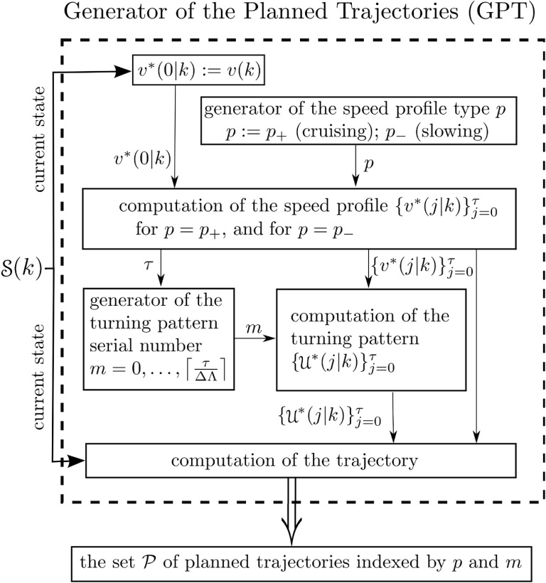
Figure 3.2: Generator of the planned trajectories.

3.2.4 Trajectory Tracking

While the planning algorithm specified in the previous section is largely similar for each vehicle model, the TTM is completely different for holonomic and unicycle vehicle kinematic models.

Holonomic

In this case the TTM updates at the same rate as the TPM, as is only invoked after the failure of the trajectory planning algorithm to find a feasible trajectory (which implies that the set $\mathscr{P}$ is empty, and thus a trajectory was inherited from the previous time-step).

Since this inherited trajectory might be traced for an extensive period of time, external disturbances may cause essential tracking errors. To compensate for this, the corrective control $\boldsymbol{u}_{f}(k)$ is added to the planned one, and so the overall control is as follows:

$$\boldsymbol{u}(k)=\boldsymbol{u}^{*}(0|k)+\boldsymbol{u}_{f}(k),$$ (3.15)

The corrective control is formed by a linear feedback with saturation at the level $u_{exc}:=(1-\mu)u_{max}$ from Eq.(3.4):

$$\boldsymbol{u}_{f}(k)=\text{\bf sat}^{u_{exc}}_{u_{exc}}\big{[}k_{0}\bar{\boldsymbol{s}}(k)+k_{1}\bar{\boldsymbol{v}}(k)\big{]}.$$ (3.16)

Here $\bar{\boldsymbol{s}}$ and $\bar{\boldsymbol{v}}$ are attributed to the difference between the vehicle current state and the predicted state on the trajectory being followed.

For given $u_{exc}$ and $w_{max}$, the gain coefficients $a_{pos}$ and $a_{vel}$ from Eq.(3.16) were optimized for minimum distance deviation under disturbance. This leads to a value of the maximum positional error $d_{trk}$, which can be computed in a similar manner as the robustly positively-invariant set [268].

There is some trade-off between the optimal distance deviation $d_{trk}$ and the tunable maximum excess control input $u_{exc}$.

By following Lemma 3.2.1, it can be guaranteed that whenever the last planned trajectory was feasible, the vehicle never moves closer than $d_{sfe}$ to the obstacle.

Remark 3.2.3

In the model Eq.(3.1), the additive disturbance $\boldsymbol{w}(k)$ accounts for the un-modeled dynamics of the system, along with other factors. Whenever the overall ‘disturbance’ obeys the adopted upper bound, the above discussion argues the robustness of the navigation law against the entire totality of uncertainties; the deviation from the planned trajectory does not exceed $d_{trk}$. It however does not exclude that within this bound, behaviors like systematic deviation from or oscillation about the planned trajectory may occur. If they yet occur and are undesirable, further elaboration of the navigation law may be required.

An example of optimal feedback gains and positional errors for a particular set of parameters is presented in Table 3.1.

$u_{exc}$	$0.4$
$w_{max}$	$0.2$

$k_{0}$	$1.33$
$k_{1}$	$0.667$
$d_{max}$	$0.30$

Table 3.1: Trajectory tracking parameters for a holonomic vehicle.

It remains to discuss one special case that is not covered by the above instructions: the last planned trajectory is exhausted, but the trajectory planning algorithm still fails. Since the planned probational velocity is zero, and the control Eq.(3.16) is employed, the actual vehicle speed is typically small in this case. This leads to the possibility of a deadlock-type behavior. While it may be possible rely on a more complete trajectory planning method in these circumstances, it cannot be generally guaranteed that a feasible trajectory exists, since the evolution of the sensed free space $F_{vis}(k)$ was not characterized. A solution is presented in Chapt. 4 which uses a better characterization of $F_{vis}(k)$, and an alternative solution is explored in Chapt. 6, which uses a navigation function to prevent deadlock.

Unicycle

A more sophisticated trajectory tracking controller is required for unicycle vehicles, due to the reduced maneuverability and nonlinear constraints. In this section a sliding mode control law is used to perform the compensation.

To compensate for space errors, the sliding mode path tracking approach presented in [220] is adopted (this is included in Chapt. 9). This navigation law is designed for pure steering control of a car-like vehicle governed by bicycle kinematics, traveling at the constant nominal longitudinal speed. Chosen for its provable bounds on tracking error in the face of a bounded wheels slip, this navigation law is adapted for trajectory tracking purposes in this chapter. In particular, a Longitudinal Tracking Module (LTM) must be added to the Path Tracking Module (PTM) to maintain the temporal difference between the planned and actual positions. Other examples of navigation approaches suitable for this task include, MPC based trajectory tracking (see e.g. [118]).

Path Tracking

Three types of disturbance are considered in Eq.(3.2) – bias in the longitudinal acceleration, bias in the turning rate, and a side slip causing an angular difference between the vehicle orientation and the velocity direction.

The proposed trajectory tracking strategy belongs to the class of sliding mode control laws [339]. Due to the well-known benefits such as high insensitivity to noises, robustness against uncertainties, and good dynamic response [339], the sliding mode approach attracts a growing interest in the area of motion control. The major obstacle to implementation of sliding mode controllers is a harmful phenomenon called ”chattering”, which is undesirable finite frequency oscillations around the ideal trajectory due to un-modeled system dynamics and constraints. The problem of chattering elimination and reduction has an extensive literature (see e.g. [84, 184]). It offers a variety of effective approaches, including smooth approximation of the discontinuity, insertion of low-pass observers into the control loop, the combination of sliding mode and adaptive control or fuzzy logic techniques, and higher order sliding modes. Whether chattering be encountered in applications of the proposed controller, it can be addressed using these techniques.

In these simulations and experiments, the discontinuous signum function employed by the navigation law was replaced with the saturated linear function $\text{\bf sat}^{+1}_{-1}(\cdot)$. This was found to give more than satisfactory performance during trajectory tracking.

Figure 3.3: The trajectory tracking model of the unicycle.

Since PTM updates controls at much higher rate than TPM, the continuous-time model of the vehicle motion is now employed. Furthermore, since disturbances are the main concern now, they are included in Eq.(3.2). To come into details, the following variables are introduced (see Fig. 3.3):

• $\eta$ – the curvilinear abscissa of the point on the reference path closest to the robot;

• $\boldsymbol{r}(\eta)\in\mathbb{R}^{2}$ – a regular parametric representation of the reference path in the world frame;

• $\varkappa(\eta)$ – the signed curvature of the reference path at the point $r(\eta)$;

• $z$ – the distance from the robot to the reference path;

• $\varphi$ – the angular difference between the robot orientation and the velocity direction caused by the wheels slip;

• $\hat{\theta}$ – the angle between the vehicle orientation and the orientation of a virtual vehicle perfectly tracking the reference path, positioned on $r(\eta)$;

• $w_{\theta}$ – the coefficient of the rotation rate bias due to disturbance;

• $w_{v}$ – the longitudinal acceleration bias due to disturbance.

Lemma 3.2.2

The trajectory tracking kinematic model is as follows:

$$\dot{\eta}=\frac{v\cos(\hat{\theta}-\varphi)}{1-\varkappa(\eta)z},\;\dot{z}=-v\sin(\hat{\theta}-\varphi),$$ (3.17a)

$${\dot{v}=\begin{cases}u_{v}+w_{v}&\text{\rm if}\;0<v<v_{max}\;\;\;\text{\rm or}\;\left\{\begin{array}[]{l}v=0\\ u_{v}+w_{v}>0\end{array}\right.\;\text{\rm or}\;\left\{\begin{array}[]{l}v=v_{max}\\ u_{v}+w_{v}<0\end{array}\right.\\ 0&\text{\rm otherwise}\end{cases}}$$ (3.17b)

$$\dot{\hat{\theta}}=\varkappa(\eta)\frac{v\cos(\hat{\theta}-\varphi)}{1-\varkappa(\eta)z}+u_{\theta}+{v}w_{\theta}.$$ (3.17c)

The proof of this lemma is similar to that of Lemma 3.1 from [239], where the bicycle error tracking model is presented. To adapt this model to the case at hand, it suffices to put $u_{\theta}+{v}w_{\theta}$ in place of $\frac{v}{L}\left[\tan(\delta+\beta)-\tan\varphi\right]$ and take into account the differences between a unicycle and bicycle, as well as that the velocity is now actuated.

To generate the steering control signal, the navigation law from Chapt. 9 is employed, slightly adopted to the current context:

$$u_{\theta}(t)=\boldsymbol{sat}_{-u_{\theta,max}}^{\phantom{-}u_{\theta,max}}\left[v\frac{\varkappa_{\text{v}}-p(\lvert S\rvert,z)}{\varkappa_{\text{v}}-\underline{\varkappa}(z)}\Xi+vp(\lvert S\rvert,z)\text{\bf sgn}(S)\right],$$ (3.18)

$$\text{where}\quad\Xi:=\frac{\varkappa(\eta)\cos(\hat{\theta})}{1-\varkappa(\eta)z}+\frac{d\chi}{dz}(z)\sin(\hat{\theta}),\quad S:=\hat{\theta}-\chi(z).$$

Here the lower bound $\varkappa_{max}$ on the reference path curvature is given by Eq.(3.5). The functions $\chi(z)$, $p(\lvert S\rvert,z)$ and $\underline{\varkappa}(z)$ are user selectable, subject to some restrictions described in Chapt. 9.

Assumption 3.2.1

There exists a choice of the coefficients $\mu$ (with indices) from Eq.(3.4), Eq.(3.12) and functions $\chi(z)$, $p(\lvert S\rvert,z)$, and $\underline{\varkappa}(z)$, such that all assumptions from Chapt. 9 hold.

These assumptions employ some constants, which are as follows in the context of this chapter: $\overline{\varphi}:=\varphi_{max},\varphi_{est}:=\varphi_{max},\varkappa_{v}:=\varkappa_{max},\overline{\varkappa}:=\mu_{\varkappa}\varkappa_{max},\varkappa_{v,\boldsymbol{u}}:=\varkappa_{max}-w_{\theta,max}$.

Constructive sufficient conditions for Assumption 3.2.1 to hold, as well as details of the required functions may be found in Chapt. 9. At the same time, it may be noted that these conditions can be satisfied by proper choice of the coefficients $\mu_{u},\mu_{\theta},\mu_{v}$ in Eq.(3.4), provided that minor and partly unavoidable requirements are met. According to Chapt. 9, the resultant tracking errors $\overline{z}_{err}\geq|z|$ ($\overline{z}_{est}$ in notations of Chapt. 9) and $\overline{\theta}_{err}\geq|\hat{\theta}|$ are explicitly determined by these coefficients (for given parameters of the vehicles) and are not influenced by both the path selected by TPM and the speed profile $v(\cdot)$. It is worth noting that typically $\overline{z}_{err}\mu_{\varkappa}\varkappa_{max}\ll 1$ and $\overline{\theta}_{err}+\varphi_{max}\ll\pi/2$ (see Chapt. 9).

Longitudinal Tracking

Longitudinal tracking adjusts the vehicles speed so the correct position along the trajectory is maintained throughout path tracking. Though the trajectory to be tracked is given by the sequence of way-points, it can be easily interpolated on any interval between sampling times to give rise to its continuous-time counterpart. The related variables will be marked by ^∗. Whereas PTM makes the curvilinear ordinate $z$ close to that $z^{\ast}=0$ of the traced trajectory, the goal of LTM is to equalize the abscissas $\eta$ and $\eta^{\ast}$. To this end, the following longitudinal tracking controller is employed:

$$u_{v}(t)=u_{v}^{\ast}(t)-u_{v,exc}\;\text{\bf sgn}\Big{\{}k_{0}\big{[}\eta-\eta^{\ast}(t)\big{]}+k_{1}\big{[}v-v^{\ast}(t)\big{]}\Big{\}},$$ (3.19)

$$\text{where}\quad u_{v,exc}:=u_{v,max}-u_{v,nom}\overset{\text{Eq.\eqref{v.nom}}}{=}\big{(}1-\mu_{u}\big{)}u_{v,max}>0$$

Here $k_{i}>0$ are tunable controller parameters. In order that the longitudinal control be realistic, the vehicle should be controllable in the longitudinal direction, i.e., the available control range exceeds that of disturbances: $u_{v,max}>w_{v,max}$.

Proposition 3.2.1

Suppose that the controller parameters $\mu_{u}\in(0,1),k_{0}>0,k_{1}>0$ are chosen so that :

$$u_{v,exc}>w_{v,max},\quad u_{v,exc}-w_{v,max}>\frac{k_{0}}{k_{1}}\left[2v_{max}+w_{\eta,max}\right],$$ (3.20)

where

$$w_{\eta,max}:=\frac{\overline{z}_{err}\mu_{\varkappa}\varkappa_{max}+1/2\left(\overline{\theta}_{err}+\varphi_{max}\right)^{2}}{1-\overline{z}_{err}\mu_{\varkappa}\varkappa_{max}}.$$ (3.21)

Then the maximum longitudinal deviation $|\eta-\eta^{\ast}|$ along the trajectory is bounded by $\frac{k_{1}w_{\eta,max}}{k_{0}}$.

Proof

First put $\eta_{\Delta}(t):=\eta(t)-\eta^{\ast}(t),v_{\Delta}(t):=v(t)-v^{\ast}(t),S:=k_{0}\eta_{\Delta}+k_{1}v_{\Delta}$ and note that due to Eq.(3.17a) and Eq.(3.17b),

$$\dot{\eta}_{\Delta}=\frac{v\cos(\hat{\theta}-\varphi)}{1-\varkappa(\eta)z}-v^{\ast}=v_{\Delta}+w_{\eta},$$ (3.22)

$${\dot{v}_{\Delta}=\begin{cases}\sigma:=-u_{v,exc}\,\text{\bf sgn}(S)+w_{v}&\text{\rm if}\;0<v<v_{max}\;\text{\rm or}\;\left|\begin{array}[]{l}v=0\\ \sigma>0\end{array}\right.\;\text{\rm or}\;\left|\begin{array}[]{l}v=v_{max}\\ \sigma<0\end{array}\right.\\ -\boldsymbol{u}^{\ast}_{v}(t)&\text{\rm otherwise}\end{cases}}$$

In Eq.(3.22),

$$w_{\eta}:=\frac{v\cos(\hat{\theta}-\varphi)}{1-\varkappa(\eta)z}-v\Rightarrow|w_{\eta}|\overset{\text{Eq.\eqref{w.eta}}}{\leq}w_{\eta,max}.$$

First it is shown in the domain $0<v<v_{max}$, the discontinuity surface $S=0$ is sliding. Indeed, in a close vicinity of any concerned point, it follows:

$$\dot{S}\,\text{\bf sgn}(S)=\left[k_{0}\dot{\eta}_{\Delta}+k_{1}\dot{v}_{\Delta}\right]\,\text{\bf sgn}(S)=k_{1}(-u_{v,exc}+w_{v}\,\text{\bf sgn}(S))+k_{0}(v_{\Delta}+w_{\eta})\,\text{\bf sgn}(S)\\ \leq-k_{1}(u_{v,exc}-w_{v,max})+k_{0}(|v_{\Delta}|+|w_{\eta}|)\leq-k_{1}(u_{v,exc}-w_{v,max})+k_{0}(2v_{max}+w_{\eta,max})\\ \leq-k_{1}\left[\big{(}1-\mu_{u}\big{)}u_{v,max}-w_{v,max}\right]+k_{0}(2v_{max}+w_{\eta,max})\overset{\text{Eq.\eqref{c.par}}}{<}0.$$

According to the architecture of the proposed navigation system, the reference trajectory always starts at the real state. So tracking is commenced with zero error $\eta_{\Delta}=0,v_{\Delta}=0$, i.e., on the sliding surface. Hence tracking proceeds as sliding motion over the surface $S=0$ while $0<v<v_{\max}$. During this motion,

$$S=k_{0}\eta_{\Delta}+k_{1}v_{\Delta}=0\Rightarrow v_{\Delta}=-\frac{k_{0}}{k_{1}}\eta_{\Delta}\overset{\text{Eq.\eqref{eq4}}}{\Rightarrow}\dot{\eta}_{\Delta}=v_{\Delta}+w_{\eta}=-\frac{k_{0}}{k_{1}}\eta_{\Delta}+w_{\eta}\\ \Rightarrow\eta_{\Delta}(t)=\int_{0}^{t}e^{-\frac{k_{0}}{k_{1}}(t-\tau)}w_{\eta}(\tau)\;d\tau\Rightarrow|\eta_{\Delta}(t)|\leq\int_{0}^{t}e^{-\frac{k_{0}}{k_{1}}(t-\tau)}w_{\eta,max}\;d\tau\leq\frac{k_{1}w_{\eta,max}}{k_{0}}.$$

Now the marginal cases where $v=0$ or $v=v_{max}$ are analyzed. If a state where $v=0$ is reached with $\eta<\eta^{\ast}$, it follows $\sigma=-u_{v,exc}\,\text{\bf sgn}\,\left[k_{0}(\eta-\eta^{\ast})-k_{1}v_{\ast}\right]+w_{v}>0$. Then the formula for $\dot{v}_{\Delta}$ is identical to that in the domain $0<v<v_{max}$, and the above analysis remains valid. If conversely, $\eta\geq\eta^{\ast}$, the vehicle is steady $\dot{\eta}=0$, whereas $\dot{\eta}_{\ast}\geq 0$, so the error $\eta-\eta^{\ast}$ does not increase. If a state where $v=v_{max}$ is reached with $\eta>\eta^{\ast}$, it follows $\sigma=-u_{v,exc}\,\text{\bf sgn}\,\left[k_{0}(\eta-\eta^{\ast})+k_{1}(v_{max}-v_{\ast})\right]+w_{v}<0$, and the arguments concerning the domain $0<v<v_{max}$ remain valid. If conversely, $\eta\leq\eta^{\ast}$, the vehicle moves at the maximal speed $\dot{\eta}=v_{max}$, whereas $\dot{\eta}_{\ast}\leq\mu_{v}v_{max}<v_{max}$, so the error $\eta-\eta^{\ast}$ decrease.

Thus the longitudinal deviation does not exceed $\frac{k_{1}w_{\eta,max}}{k_{0}}$ in any case. $\quad\bullet$

It should be noted that conditions Eq.(3.20) can always be satisfied by proper choice of the controller parameters $\mu_{v},k_{0},k_{1}$. In conclusion, it is noted that the overall positional deviation $\lVert\boldsymbol{s}(t)-\boldsymbol{s}^{\ast}(t)\rVert$ between the actual and reference trajectories does not exceed $|z|+|\eta-\eta^{\ast}|$. So the estimate introduced in Sec. 3.2.2 can be taken in the form:

$$d_{trk}=\overline{z}_{est}+\frac{k_{1}w_{\eta,max}}{k_{0}}.$$ (3.23)

3.2.5 Implementation Details

The selection of the trajectory from $\mathscr{P}$ is arbitrary – any possible choice of cost functional will not alter the collision avoidance properties. In addition this cost functional could also be used with other optimization routines, which would likely result in similar results. For this implementation, the trajectory from $\mathscr{P}$ was chosen minimizing of the cost functional:

$$J:=\lVert\boldsymbol{s}^{*}(\tau|k)-T\rVert-\gamma_{0}\lvert v^{*}(1|k)\rvert.$$ (3.24)

Here $\gamma_{0}>0$ is a given tunable parameter. This minimization aims to achieve the best progression to the target and to simultaneously increase the speed at the first time step, and was found to give excellent experimental results for both holonomic and unicycle vehicles.

3.3 Simulations

For these simulations, both holonomic and unicycle vehicle models were employed, and the controller sampling time was set to unity. The parameters used for navigation can be found in Tables 3.2 and 3.3. The visible region $F_{vis}(k)$ was taken to be the points from $F$ within $4m$ of the vehicle, which also had line-of-sight visibility to the vehicle through $F$. As may be seen in Figs. 3.4 to 3.7, the proposed method was able to guide the vehicle satisfactorily without collision for both the vehicle models.

$u_{max}$	$1.0ms^{-2}$
$u_{nom}$	$0.5ms^{-2}$
$u_{sp}$	$0.2ms^{-1}$

$d_{tar}$	$0.5m$
$v_{max}$	$1.0ms^{-1}$
$\gamma_{0}$	$10$

Table 3.2: Simulation parameters for holonomic controller.

Figure 3.4: Trajectory obtained using the basic controller with a holonomic vehicle model.

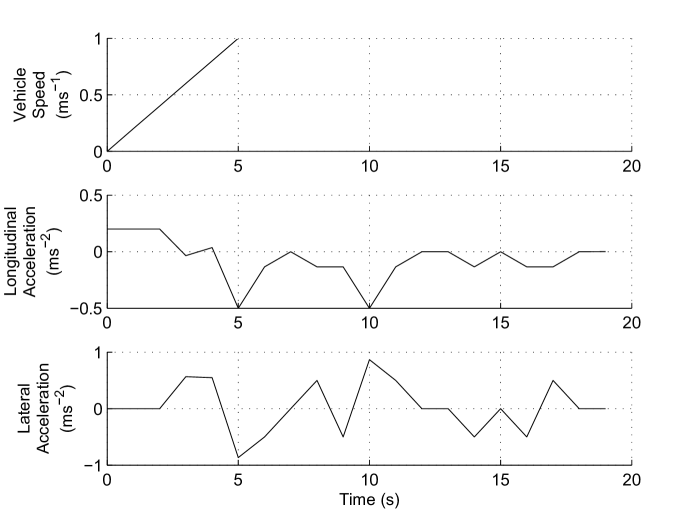
Figure 3.5: Control time history of the basic controller with a holonomic vehicle model.

Figs. 3.5 and 3.7 show that in this case, the vehicle accelarated to the maximum speed and mostly stayed around this speed. In later chapters (Chapts. 4 to 6) where more complicated scenarios are considered, more speed fluctations will be required to give the vehicles more maneuverability when avoiding obstacles.

$d_{tar}$	$0.5m$
$v_{max}$	$1.1ms^{-1}$
$u_{\theta,max}$	$0.6rads^{-1}$
$u_{v,max}$	$0.3ms^{-2}$
$v_{nom}$	$1.0ms^{-1}$
$u_{\theta,nom}$	$0.5rads^{-1}$

$u_{v,nom}$	$0.2ms^{-2}$
$\Delta\Lambda$	$0.5$
$k_{0}$	$1$
$k_{1}$	$1$
$\gamma_{0}$	$10$
$\mu_{\varkappa}$	$0.9$

Table 3.3: Simulation parameters for unicycle controller.

Figure 3.6: Trajectory obtained using the basic controller with a unicycle vehicle model.

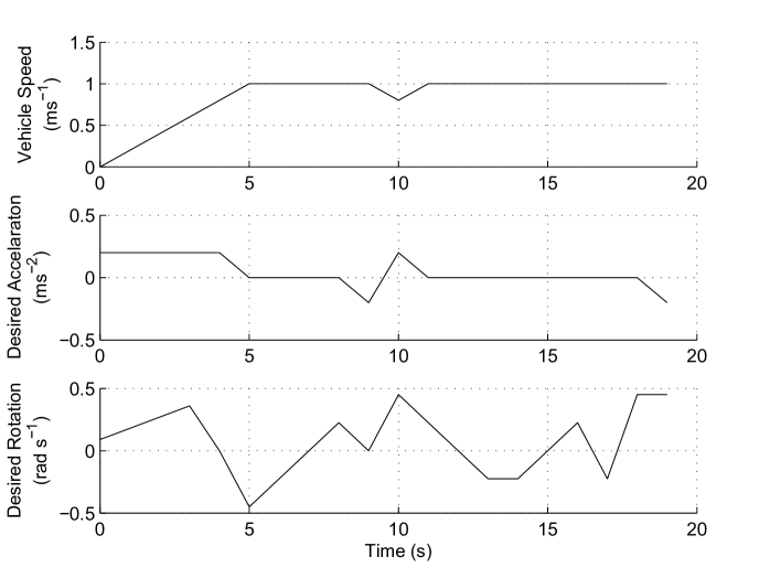
Figure 3.7: Control time history of the basic controller with a unicycle vehicle model.

3.4 Summary

In this section, the basic navigation framework which achieves collision avoidance is presented. By combining a simplified trajectory planning scheme and a robust MPC type navigation approach, collision avoidance can be proven under bounded disturbance, for both holonomic and unicycle vehicle motion models, when static obstacles are present.

Chapter 4 Collision Avoidance with Limited Sensor Information

In this chapter, the previous navigation system is extended to cases where only sampled information about the obstacle boundary is available, similar to what would be obtained from a LiDAR device. Here the problem of following an obstacle boundary in a convergent manner is considered, however this approach could easily be extended to general collision avoidance, and a possible method of achieving target convergent navigation is outlined. Additionally, a possible extension allowing avoidance of moving obstacles is provided.

By forming some assumptions about both the shape of the obstacle and the resolution of the obstacle sensor, constraints suitable for navigation using a MPC type approach are generated. An algorithm for selecting a target point to enable navigation in-line with the goal of boundary following is also proposed. Overall this leads to a navigation system more suitable for real world implementation, compared with the system from Chapt. 3.

The body of this chapter is organized as follows. In Sec. 4.1 the problem is formally defined, and in Sec. 4.2 the navigation approach is described. A method of extending the controller to target convergence problems is described in Sec. 4.3, and to moving obstacle in Sec. 4.4. Simulations and experiments are presented in Secs. 4.5 and 4.6. Finally, brief conclusions are given in Sec. 4.7.

4.1 Problem Statement

A single vehicle with unicycle kinematics traveling in a plane is considered, which contains a single static obstacle $D$. It is assumed $D$ is simply connected, and thus does not enclose the vehicle. The boundary of $D$ is denoted $\partial D$, which is assumed to have continuous curvature. The desired transversal direction is given, which is encoded by the variable $\Gamma\in\{-1,+1\}$, where clockwise corresponds to $-1$ and counterclockwise corresponds to $+1$. The opposite direction $\bar{\Gamma}$ is referred to as the anti transversal direction.

The distance to be maintained from any possible obstacle point during planning is $d_{rad}$. Due to the quantized nature of the range data available, the navigation approach cannot plan vehicle positions arbitrarily close to the obstacle. Thus a user selectable threshold $d_{tar}>d_{rad}$ is introduced, and navigation between two adjacent obstacle segments is guaranteed if the minimum distance between them is greater than $2d_{tar}$. The value of $d_{tar}$ partially determines the sensing and obstacle requirements, and the margin between $d_{tar}$ and $d_{rad}$ is denoted $d_{ob}:=d_{tar}-d_{rad}$.

In this problem, the obstacle boundary $\partial D$ should be tracked so that any point on $\partial D$ is within a distance $2d_{tar}$ of at least one detected point on the obstacle at some time during the transversal. In a obstacle avoidance problem this could be interpreted as assurance that any corridors, possibly leading to the target, will be transversed.

In this chapter, only the unicycle model is considered for brevity, through these results could easily be extended to the holonomic model. Also for brevity, the system is assumed free from disturbance – extending these results to cases where disturbance is present remains a topic of future research. As the open loop control inputs can be applied directly without employing the TTM, there is no need for measurement of the vehicles position $\boldsymbol{s}(k)$ and heading $\theta(k)$. However it is assumed at every time $k$, every vehicle has knowledge of its speed $v(k)$ (as required by the TPM).

4.1.1 Obstacle Requirements

It is necessary to characterize the obstacle so that the resolution requirements of the range sensor can be formulated. More contorted obstacles would have greater sensing requirements than smooth obstacles in order to navigate successfully. The first requirement is concerned with preventing collisions:

Requirement 4.1.1

The distance $d_{ob}$ is required to be sufficiently large such that for any point $\boldsymbol{p}_{1}\in\partial D$, there exists another point $\boldsymbol{p}_{2}$ separated by a distance $d$, $0<d\leq d_{ob}$, such that exactly one of the two boundary segments connecting them lies completely within $d_{ob}$ of both points for any $\boldsymbol{p}_{2}$.

Requirement 4.1.1 is demonstrated in Fig. 4.1. This excludes narrow obstacle protrusions, which may not be detected in some circumstances and cause a collision.

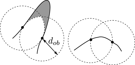
Figure 4.1: Obstacle boundary assumption related to $d_{ob}$.

The next definition is similar to Requirement 4.1.1 in that it provides a bounded area which the obstacle boundary must lie within between two points. While the last definition was focused on safety, the following ensures the overall navigation objective can be achieved:

Requirement 4.1.2

The distance $d_{tar}$ is required to be sufficiently large such that for any point $\boldsymbol{p}_{1}\in\partial D$, there exists another point $\boldsymbol{p}_{2}$ separated by a distance $d$, $0<d\leq 2d_{tar}$, such that at least one of the two boundary segments connecting the points must lie completely within $2d_{tar}$ of either point for any $\boldsymbol{p}_{2}$.

This requirement is demonstrated in Fig. 4.2 and avoids long narrow corridors which may be skipped by the vehicle resulting in incomplete navigation.

Figure 4.2: Obstacle boundary assumption related to $d_{tar}$.

4.1.2 Sensor Model

At every time step $k$, the vehicle emanates a finite sequence of $N_{r}$ rays radially around it, with a constant angular spacing $\Delta\varphi=\frac{2\pi}{N_{r}}$ between them. The vehicle has knowledge of the point $R_{i}$ for which each ray first intersects an obstacle, $i=1:N_{r}$. These points are taken from the vehicles reference frame, so that the distance from $R_{i}$ to the vehicle may be given by $\lVert R_{i}\rVert$. Also, for convenience the notation is wrapping, i.e. $R_{i}\equiv R_{i\pm N_{r}}$.

Assumption 4.1.1

It is assumed that the range sensor has a maximum detection radius of $R_{sen}$, which means $R_{i}$ is unknown if $\lVert R_{i}\rVert>R_{sen}$. This maximum range is tightened based on the obstacle feature size, and the effective maximum detection radius $R_{max}$ is defined as follows:

$$R_{max}:=\min\left\{R_{sen},\frac{d_{ob}}{\sqrt{\frac{8}{3}(1-\cos(\Delta\varphi))}}\right\}$$ (4.1)

It is also assumed $R_{max}$ is greater than $4d_{tar}$.

The denominator in Eq.(4.1) arises during analysis; its origin may be found in the proof of Lemma 4.2.1.

4.1.3 Concluding Remarks

The distances employed by the navigation law are summarized in Fig. 4.3. In this figure, since all circles of radius $d_{tar}$ overlap, Requirement 4.1.2 applies to every pair of points. This means the protruding part of the obstacle must lie within $2d_{tar}$ of every pair of points. Also, the circles of radius $d_{ob}$ cover subsequent detection points, except for the center detection ray. This means between these points a bounded area which contains the obstacle boundary may be expressed, according to Requirement 4.1.1. A circle of radius $d_{rad}$ is also shown around the vehicle, which must exclude any point which is potentially part of the obstacle (see Algorithm 4.2.1).

Figure 4.3: Relationship between the distances employed by the navigation law.

Remark 4.1.1

Note Requirement 4.1.1 is automatically fulfilled if the boundary curvature radius is greater than $\frac{1}{2}d_{ob}$. This limit would also eliminate small protrusions which may not be detected by the obstacle sensor, through it should be emphasized the curvature does not need not be bounded for Requirement 4.1.1 to hold. Also note Requirement 4.1.2 may be omitted if the entire boundary is not required to be covered by the vehicle.

4.2 Navigation System Architecture

The idea behind this approach is to make the vehicle move towards the edge of the points that are known to be part of a solid obstacle boundary, while adjusting the speed to avoid collisions. As in Chapt. 3 a type of receding horizon control is employed, but in this case the probational trajectories are constrained to achieve the navigation objective.

As in Chapt. 3, a probational trajectory commencing at the current system state is found over a variable finite horizon at every time instant $k$. As before, this probational trajectory is specified by a finite sequence of way-points, which satisfy the constraints of the vehicle model. Probational trajectories necessarily have zero velocity at the terminal planning time, which ensures availability of at least one safe probational trajectory at subsequent time steps.

Trajectory generation may potentially use many different forms, through in the implementation presented in this chapter, the planning algorithm proposed in Chapt. 3 is used.

There are two caveats for the trajectory planning system:

• Firstly, regardless of the path planning method employed,assume the probational trajectory may be inherited from the previous time-step. The reasoning is the constraints are time-altering, this it is unknown whether a feasible trajectory exists at any particular time; the inherited trajectory was subject to constraints from a previous time-step and thus is independent of the current ones.

• Secondly, the algorithm may alternatively select specifically prescribed trajectory, which is formulated in Lemma 4.2.3. This may be regarded as a contingent ‘recovery scheme’, which can guarantee a trajectory is always available when the vehicle is stationary.

The final algorithm consists of sequential execution of the following steps:

1. Construction of the constraints based on the range detections. These include avoidance constraints (see Sec. 4.2.1) and convergence constraints (see Sec. 4.2.2).

2. Arbitrary selection of a probational trajectory satisfying constraints.

3. Application of the first control $\mathscr{U}^{*}(0|k)$ related to the selected probational trajectory to the vehicle.

4. $k:=k+1$ and go to S.1.

Note in this formulation, the best choice of the probational trajectory from those which satisfy constraints is purely arbitrary. The optimal trajectory based on the given sensor information would likely depend on guessing the shape of the unknown part of the obstacle, and this characterization would likely be non-trivial (and may be an area of future research). The simplified heuristic used in for testing in this chapter may be found in Sec. 4.2.4.

It is assumed the vehicle initially can plan a feasible probational trajectory:

Assumption 4.2.1

Initially at $k=0$, at least one detection ray intersects the obstacle, and the distance from the obstacle exceeds $d_{tar}$.

Trajectory related variables depend on two arguments $(j|k)$, where $k$ is the time instant when the probational trajectory is generated and $j\geq 0$ is the number of time steps into the future; the related value concerns the state at time $k+j$. Note all points are given from the vehicles reference frame, and the origin is denoted $O$.

4.2.1 Avoidance Constraints

The first step in determining trajectory feasibility is finding the regions of the surroundings guaranteed to be obstacle free. This deliberation is based on Requirement 4.1.1; the algorithm for determining this is described as follows:

Algorithm 4.2.1

Given a point $\boldsymbol{p}$ which bisects the two adjacent obstacle detection rays associated with $R_{i}$ and $R_{i+1}$ for some $i$. There are several cases:

$\boldsymbol{R}_{i}$ and $\boldsymbol{R}_{i+1}$ defined: Assume $\lVert R_{i}\rVert\leq\lVert R_{i+1}\rVert$ (A similar argument follows if $R_{i+1}$ is nearer the vehicle than $R_{i}$), and define $d_{i}:=\lVert R_{i}-R_{i+1}\rVert$;

1) If $\lVert\boldsymbol{p}\rVert>(R_{max}-d_{ob})$, $\boldsymbol{p}$ is labeled a potential obstacle.

2) Else if $d_{i}\leq d_{ob}$, and the minimum distance from the line segment $\overline{O\boldsymbol{p}}$ to $R_{i}$ and the minimum distance from $\overline{O\boldsymbol{p}}$ to $R_{i+1}$ are both less than $d_{i}$, $\boldsymbol{p}$ is labeled a potential obstacle.

3) Else, construct a circle of radius $d_{ob}$ centered on $R_{i}$. Intersect this with the detection ray associated with $R_{i+1}$ and choose the intersection point furthest from the vehicle, labeled $\boldsymbol{q}$. If the minimum distance from $\overline{O\boldsymbol{p}}$ to $\boldsymbol{q}$ and the minimum distance from the line segment $\overline{O\boldsymbol{p}}$ to $R_{i}$ are both less than $d_{ob}$, $\boldsymbol{p}$ is labeled a potential obstacle.

4) Otherwise $\boldsymbol{p}$ is not a potential obstacle.

$\boldsymbol{R}_{i}$ defined and $\boldsymbol{R}_{i+1}$ not defined: Employ steps 1, 3 and 4 only.

$\boldsymbol{R}_{i}$ and $\boldsymbol{R}_{i+1}$ not defined: Employ steps 1 and 4 only.

Conversely the point is safe if it can be assumed to clear the set of potential obstacles by the minimum distance $d_{rad}$. An example of the results obtained using this method is illustrated in Fig. 4.4. In this figure the regions which must be assumed to be part of the obstacle are highlighted in dark gray, while the areas which can be assumed to be obstacle free are highlighted in light gray.

Proposition 4.2.1

If point $\boldsymbol{p}$ is deemed not a potential obstacle by Algorithm 4.2.1, it is in fact not part of the obstacle.

Proof

First, note adjacent range readings are sufficient to determine if a point is a potential obstacle as $\partial D$ cannot intersect the line segment $\overline{OR_{i+1}}$. When $d_{i}<d_{ob}$ the result follows directly from Assumption 4.1.1. When $d_{i}>d_{ob}$, a section of $\partial D$ must pass through a arc of radius $d_{ob}$ centered on $R_{i}$, between the adjacent detection rays, on the far side from the vehicle. In the worst case it will pass through the intersection of the arc and $\overline{OR_{i+1}}$, which is how the result follows from Assumption 4.1.1. If the distance $\lVert\boldsymbol{p}\rVert$ is greater than $R_{max}-d_{ob}$, and the first two rules have not eliminated it, it indicates $\lVert R_{i}\rVert$ and $\lVert R_{i+1}\rVert$ are both larger than $R_{max}$. The sensor may not be able to detect obstacles further than $R_{max}$ as they either are outside the range of the sensor or $\lVert R_{i}-R_{i+1}\rVert>d_{ob}$, so that Assumption 4.1.1 no longer applies. $\quad\bullet$

Note that any potential probational trajectory must lie completely with the set of currently sensed safe points.

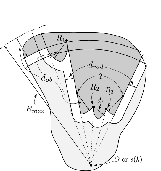
Figure 4.4: The regions which are assumed to be part of the obstacle.

Remark 4.2.1

Note a computational issue may be encountered when determining whether a probational trajectory meets avoidance constraints. The easiest method of computing whether a probational trajectory is safe involves sampling it at a sufficiently high resolution, then applying the test from Proposition 4.2.1 on each point. By doing this, there are no sampling effects related to the maximum velocity, as there were in Chapt. 3

4.2.2 Convergence Constraints

The constraints in this section ensure the vehicle make at least a non-zero movement along the obstacle boundary. To do this two definitions are introduced; the contiguous points, which is a set of adjacent range detections near the vehicle, and the target point, which is calculated to ensure progression along the boundary. Firstly, the definition of the contiguous point set is introduced:

Definition 4.2.1

The point $C_{end}(0)$ is a arbitrary valid obstacle detection taken before the navigation program commences. The set of contiguous points $C(k)$ is defined by first selecting the obstacle detection nearest $C_{end}(k-1)$. Once this point is found, adjacent obstacle detections that are within an Euclidean distance of $2d_{tar}$ with respect to any element from the current set of points can then be sequentially included. The final point to be included in $C(k)$ is labeled $C_{end}(k)$.

The purpose of finding $C(k)$ is that it can be guaranteed to be part of a obstacle boundary – it can contain no hidden corridors or gaps. Thus the vehicle can confidently navigate towards the edge of this region, which may result in a shorter trajectory and faster allowable speeds. The set $C(k)$ and its endpoint $C_{end}(k)$ are illustrated in Fig. 4.5.

Figure 4.5: Description of the contiguous set $C(k)$.

The target point is taken from a circle of radius $d_{tar}$ around $C_{end}(k)$, intersected with the next detection ray after $C_{end}(k)$. This represents the target offset distance which the vehicle may need to assume in order to track the obstacle boundary appropriately. The calculation of the target point is given as follows:

Definition 4.2.2

Let $R_{n}$ be the detected point corresponding to the next detection ray after $C_{end}(k)$ in the anti transversal direction. The target point $A(k)$ is given by:

$$A(k):=\begin{cases}\hat{R}_{n}\left(\begin{array}[]{l}\lVert C_{end}(k)\rVert\cos\Delta\varphi\\ +\sqrt{d_{tar}^{2}-(\lVert C_{end}(k)\rVert\sin\Delta\varphi)^{2}}\end{array}\right)&\lVert R_{n}\rVert>\lVert C_{end}(k)\rVert\\ C_{end}(k)&\lVert R_{n}\rVert<\lVert C_{end}(k)\rVert\end{cases}$$ (4.2)

Here $\hat{R}_{n}$ is the unit vector corresponding to $R_{n}$.

The formula follows from elementary application of the cosine rule. The target point $A(k)$ is illustrated in Fig. 4.6 (note $A(k)$ is invariably an unsafe point). To constrain the trajectory, the following convergence constraints are enforced:

1. As the vehicle moves towards $A(k)$, there exists some $b>0$, so that for all $j$ bounded by $1\leq j\leq\tau$:

   $$\lVert\boldsymbol{s}^{*}(j|k)-A(k)\rVert<\lVert A(k)\rVert-b$$ (4.3)

2. For each planned point on the probational trajectory, at least one pair of adjacent detection rays must enclose $C_{end}(k)$, without occlusion from other potential obstacles.

The second constraint would not normally significantly affect the operation of the path planning system, however it is required to prove correct operation of the navigation law.

Figure 4.6: Description of the target point $A(k)$.

4.2.3 Analysis

In this section analysis of the navigation law in achieving the stated goals is documented. The first step is to show existence and smoothness of $C(k)$:

Lemma 4.2.1

The set $C(k)$ is nonempty, the minimum pairwise distance to $C(k-1)$ is less than $2d_{tar}$, and the point $C_{end}(k)$ exists.

Proof

To show $C(k)$ is nonempty, consider a triangle of points in $\partial D$, where one point is $C_{end}(k-1)$. The other two points $\boldsymbol{p}_{1},\boldsymbol{p}_{2}$ are chosen to bisect $C_{end}(k-1)$ on $\partial D$, and also chosen so that $\lVert C_{end}(k-1)-\boldsymbol{p}_{1}\rVert=\lVert C_{end}(k-1)-\boldsymbol{p}_{2}\rVert=d_{ob}$. It is known $\lVert C_{end}(k-1)\rVert<(R_{max}-d_{tar})$, as either $\lVert C_{end}(k-1)\rVert<2d_{tar}$, or $\lVert C_{end}(k-1)\rVert$ decreased over the last time step. If there are multiple choices for these two points $\boldsymbol{p}_{1}$ and $\boldsymbol{p}_{2}$, then the points furthest away from $C_{end}(k)$ along $\partial D$ are chosen. It is clear that $\lVert\boldsymbol{p}_{1}-\boldsymbol{p}_{2}\rVert\geq d_{ob}$, since if this was not the case it would possible to select $\acute{\boldsymbol{p}}_{1}$ and $\acute{\boldsymbol{p}}_{2}$, separated by $d_{ob}$ and enclosing $\boldsymbol{p}_{1}$ and $\boldsymbol{p}_{2}$, and for which both must be further than $d_{ob}$ from $C_{end}(k)$, violating Assumption 4.1.1. It is sufficient to show intersection of this triangle corresponding to the points $\boldsymbol{p}_{1}$, $C_{end}(k-1)$, $\boldsymbol{p}_{2}$ with at least one range ray. A trigonometric argument using Assumption 4.1.1 is able to show intersection for distances up to $R_{max}$. The relation is shown in Fig. 4.7; if one of the undetected points is nearer than $R_{max}$ to the vehicle, it is evident $\sqrt{2(1-\cos(\Delta\varphi))}\cdot R_{max}>\frac{\sqrt{3}}{2}d_{ob}$ which is ascertained by Eq.(4.1), where it was assumed $R_{max}:=\min\left\{R_{sen},\frac{d_{ob}}{\sqrt{\frac{8}{3}(1-\cos(\Delta\varphi))}}\right\}$.

To show the minimum distance between $C(k)$ and $C(k-1)$ is less than $2d_{tar}$, first note the vehicle will be able to detect the triangle corresponding to the points $\boldsymbol{p}_{1}$, $C_{end}(k-1)$, $\boldsymbol{p}_{2}$. Since at least one detected point will be between the triangle and the vehicle, it will be within $2d_{tar}$ of the previous $C_{end}(k)$.

Existence of $C_{end}(k)$ follows from Requirement 4.1.2, as if the distance between every pair of adjacent range points is less than $2d_{tar}$ it indicates the obstacle is enclosing the vehicle, which is assumed to not be the case. $\quad\bullet$

Figure 4.7: Accompaniment to Lemma 4.2.1.

Next a guarantee that $A(k)$ is sufficiently spaced from the vehicle is provided. The argument is based on the geometry of the detection rays:

Lemma 4.2.2

The distance $\lVert A(k)\rVert$ is lower bounded by $d_{tar}$.

Proof

Consider a point $\boldsymbol{p}$ generated by moving $d_{tar}$ towards the origin from $A(k)$. If $\boldsymbol{p}$ is not the origin, the lemma follows. If $\lVert R_{n}\rVert>\lVert C_{end}(k)\rVert$, using Definition 4.2.2 and the fact $d_{tar}>d_{ob}$, it can be inferred $\boldsymbol{p}$ is a potential obstacle and does not coincide with the origin. When $\lVert R_{n}\rVert\leq\lVert C_{end}(k)\rVert$, note $\lVert C_{end}(k)\rVert>2d_{tar}$ and thus $\lVert A(k)\rVert>d_{tar}$. $\quad\bullet$

Next there is shown to be at least one feasible trajectory that may be produced by the algorithm. Note this trajectory is not a particularly efficient method of transversing the obstacle, it is merely to ensure the analytical claims are valid.

Lemma 4.2.3

There always exists at least one valid trajectory $\boldsymbol{s}^{*}(j|k)$

Proof

Since the trajectory from the previous time-step can always be used, the case where it is exhausted and the vehicle is stationary is considered. The recovery trajectory consists of a turn-in-place so the vehicle is aligned towards $A(k)$, followed by straight movement towards $A(k)$ of length $b$. The straight movement would be achieved by a given longitudinal acceleration at one time-step followed by an opposite deceleration at the proceeding time-step. Although the individual segments of this trajectory would not meet convergence constraints, the trajectory as a whole does. Thus the entire recovery trajectory would be executed until completion. $\quad\bullet$

Next it is shown that following feasible trajectories results in the point $C_{end}(k)$ progressing along the obstacle boundary:

Lemma 4.2.4

There exists a finite number of time steps $c_{t}$ over which time $C_{end}(k)$ will advance by at least $d_{ob}$ along the obstacle boundary.

Proof

Let $k_{c}$ refer to the time-step at the beginning of the interval for which advancement of $d_{ob}$ is being shown. Let the previous $C_{end}(k_{c})$ and $A(k_{c})$ be expressed in the vehicles current reference frame. Absurdly suppose $C_{end}(k)$ never advances by more than $d_{ob}$ along the boundary $\partial D$. It can be deduced that $C_{end}(k)$ will never regress by more than $d_{ob}$ along $\partial D$ since the triangle argument from Lemma 4.2.2 can be applied to $C_{end}(k_{c})$. Since $\lVert A(k)\rVert>d_{tar}$ it can be inferred that $\lVert C_{end}(k_{c})\rVert$ will eventually decrease below $2d_{tar}$ in finite time due to Eq.(4.3) and Lemma 4.2.3. It is known $C_{end}(k)$ lies in a disk of radius $d_{ob}$ around $C_{end}(k_{c})$. Next, define $\nu(k)$ to be the heading of $\boldsymbol{s}(k)$ from a reference frame centered at $C_{end}(k_{c})$, measured in the transversal direction from $k_{c}$ such that $\nu(k_{c}):=0$. Decreasing the distance to $A(k)$ will increase $\nu$ since all possible values of $C_{end}(k)$ are contained in a disk of radius $d_{ob}$ around $C_{end}(k_{c})$. This movement will occur in finite time due to Eq.(4.3) and Lemma 4.2.3. Once $\nu>2\pi$, the vehicle is guaranteed to sense a different side of the triangle corresponding to $C_{end}(k_{c})$. Due to the triangle side length, this advancement of $C_{end}(k)$ along the boundary is at least $d_{ob}$. The expression for $c_{t}$ would depend on $b$ from Eq.(4.3).$\quad\bullet$

Note that showing collision avoidance is elementary given the trajectories are always feasible. The final statement combines the above Lemma’s to prove the final result.

Theorem 4.2.1

The vehicle exhibits boundary following behavior, avoiding collision with the boundary while making a range reading within $2d_{tar}$ of every point on a finite obstacle boundary in finite time.

Proof

From the existence of $C_{end}(k)$ it follows the accumulated $C(k)$, given by:

$$\mathcal{C}(k):=\bigcup_{\acute{k}=0}^{k}C(\acute{k})$$ (4.4)

contains points within $2d_{tar}$ of every point on $\partial D$ between some start and end point. From Lemma 4.2.4, it follows that the span of $\mathcal{C}$ is monotonically increasing. From Lemma 4.2.2 and Lemma 4.2.4, the position of $C_{end}(k)$ along the obstacle increases by at least some increment in a finite time. Thus it may be inferred the span of $\mathcal{C}(k)$ will increase arbitrarily in a finite time, and thus the obstacle will be transversed in a finite time.$\quad\bullet$

4.2.4 Implementation Details

To implement the planning system, the same simplified planning system from Chapt. 3 is employed, and a finite set of heuristically given trajectories $\mathscr{P}$ is found. As this planning algorithm is known not to be complete, whenever $\mathscr{P}$ is empty and the inherited probational trajectory is exhausted, the trajectory used in Lemma 4.2.3 may be used in extraordinary circumstances (see Remark 4.2.2).

Only feasible trajectories may be chosen so any choice of cost functional will not alter the collision avoidance properties. For this implementation, the trajectory from $\mathscr{P}$ minimizing of the following cost functional was selected:

$$J:=\lVert A(k)-s^{*}(\tau|k)\rVert$$ (4.5)

Due to convergence constraints, any feasible trajectory will exhibit boundary following properties, thus this selection is heuristic. The formulation Eq.(4.5) was found to give good performance when implemented.

Remark 4.2.2

Simulations have demonstrated the approach described is sufficiently complete for the proposed navigation law. During the simulations and experiments in this chapter, a trajectory inheritance event was unable to be induced, so it seems somewhat unlikely that trajectories from previous time steps will be routinely employed.

4.3 Extension to Target Convergence

It is reasonably straightforward to extend the proposed navigation method to cases where a known target $T\notin D$ must be converged to in finite time. The main modification is the addition of a trajectory leading the target, which is followed whenever feasible. The reactive navigation system is somewhat similar that described in Chapt. 7. However, the ability to imitate the exact same switching conditions from ‘boundary following’ to ‘target pursuit’ would be required to show the bi-similarity of the algorithms, and an area of future research.

4.3.1 Angular Progression

Since the heading $\theta$ of the vehicle is not necessarily correlated with any parametric representation of the obstacle, other means are required to track the angular progression along the obstacle boundary. Define $\alpha$ to be the relative heading from the vehicle between $C_{end}(k)$ and the target $T$:

$$\alpha(k):=\angle(C_{end}(k)-\boldsymbol{s}^{*}(0|k))-\angle(C_{end}(k)-T)+\pi$$

Here $\angle(\cdot)$ represents the angle of a vector. The angle $\alpha(k)$ evolves continuously over time, such that it may become arbitrary large in certain types of obstacles with local minima having complicated shapes. Thus a projected value $\alpha_{\tau}(k)$ is defined, where $\boldsymbol{s}^{*}(0|k)$ is replaced with the projected position at the end of the trajectory $\boldsymbol{s}^{*}(\tau|k)$. When transitioning into boundary following mode, $\alpha$ may be reset to lie within the interval $[-\pi,\pi]$.

Figure 4.8: Relationship between $\alpha$ and $\beta$.

Define $\beta(k)$ to be the angle between a tangential ray from the obstacle at $C_{end}(k)$ in the transversal direction, and the line segment $\overline{C_{end}(k)T}$. Similarly to $\alpha(k)$, $\beta(k)$ evolves continuously over time, however it is impossible for the vehicle to calculate the exact vale of $\beta(k)$ is in general. However it is somewhat equivalent to the measurement used in Chapt. 7 to calculate mode switching conditions, so by showing $\alpha(k)$ and $\beta(k)$ are similar, it may mean some of those results are relevant.

Proposition 4.3.1

The following inequalities hold: $|\alpha(k)-\beta(k)|<\pi$ and $|\beta(k)|\geq|\alpha(k)|$

Proof

The angle of the actual tangent ray of the obstacle at $C_{end}(k)$ subtended the line segment $\overline{OC_{end}(k)}$, labeled $\nu$, is contained in the interval $[0,\Gamma\pi]$, as any other direction would require $C_{end}(k)$ to be a corner point, which is precluded by Assumption 4.1.1. By summing the angles around $C_{end}(k)$, $(\pi-\alpha(k))+\beta(k)+\nu\equiv 2\pi$, from which the proposition follows. $\quad\bullet$

In Fig. 4.8, the switching condition based on $\Gamma\cdot\alpha_{\tau}(k)$ is illustrated, while in Fig. 4.8 the correlation between $\alpha(k)$ and $\beta(k)$ is illustrated.

4.3.2 Reference Trajectory

Next, the reference trajectory is defined by the choice of navigation parameters which satisfy the following criteria:

• Monotonically decreases the distance to target relative to the current vehicle position.

• The projected $\Gamma\cdot\alpha_{\tau}(k)<0$; this is illustrated in Fig. 4.8.

• Does not violate collision avoidance constraints.

If multiple valid choices are available, a selection is made to minimize the distance to the target for the final trajectory point. Whenever the reference trajectory exists, it is used in preference to the trajectory obtained from the boundary following method. However, the contiguous set would be updated as normal during this mode (in some cases it may become empty, such as when departing an obstacle).

4.3.3 Initial Selection of Contiguous Set

Whenever boundary following is engaged, an alternative contiguous set is generated by first finding the set of obstacle detections within $d_{tar}$ of any point on the reference trajectory, then selecting the point nearest the vehicle as the seed point.

If the alternative $\acute{C}(k)$ matches the current $C(k)$, or if the alternative contiguous set is empty, it can be presumed that the vehicle is still following the same boundary segment, and no changes to the transversal direction are required. However if they are different, it must assumed that the vehicle has encountered a new boundary segment; this is demonstrated in Fig. 4.9. In this case, the transversal direction can be randomly chosen in-line with Chapt. 7.

Remark 4.3.1

It is not claimed that the proposed navigation law converges to the target in general. However due to the properties of $\alpha$, the switching condition is similar [223], so convergence to target seems likely, at least in conservative scenarios.

Figure 4.9: (a) The alternate contiguous set; (b) Constraints for moving obstacles.

4.4 Extension to Moving Obstacles

Allowance can be made for the obstacle to move with a constant translational velocity. This may have applications such as following large moving objects such as ships, or movement in environments with persistent disturbances, such as water currents and wind.

Assumption 4.4.1

The obstacle is traveling at a constant speed $v_{ob}$ in constant direction $\theta_{ob}$, which is known to the vehicle. The obstacle velocity does not exceed that of the vehicles such that $v_{ob}<v_{max}$.

While the bounds on the obstacle speed are not restrictive, lower obstacle velocities are likely to result in better performance of the algorithm. The velocity of the obstacle could be easily estimated from the range measurements. Many algorithms have been developed for this task, an example being Iterative Closest Point matching [362]. However, during the simulations presented here, the obstacle velocity was assumed to be known by the vehicle, thus a obstacle tracking algorithm was not implemented.

Collision avoidance can be predicted by subtracting the future movement of the obstacle from the future vehicle position, and applying Proposition 4.2.1 to determine interference with the obstacle as normal. There is an additional modification to the terminal constraint – the vehicle must be traveling in the same speed and direction as the obstacle at the end of the trajectory. To do this, the speed along the trajectory is not reduced beyond $v_{ob}$. The trajectory is then appended with a turn at maximal actuation aligning the vehicle heading $\theta(j|k)$ with the obstacle’s direct $\theta_{ob}$, while maintaining the same speed. This is demonstrated in Fig. 4.9.

Remark 4.4.1

It is impossible to design a trivial recovery scheme as was the case for the stationary obstacle. Because of this, correct boundary following behavior of the vehicle cannot be shown. However collision avoidance with the obstacle can still be shown, as there is zero relative movement between the vehicle and obstacle at the end of the trajectory.

4.5 Simulations

The control law was simulated using the perfect discrete time model, updated at a sample time of $1s$. The control parameters may be found in Fig. 4.1. Simulations were carried out on a 3.0 GHz Pentium processor, using MATLAB interfaced with C++ Mex files.

$u_{\theta,max}$	$0.5rads^{-1}$
$u_{v,nom}$	$0.2ms^{-2}$
$v_{max}$	$1.0ms^{-1}$

$d_{ob}$	$1.0m$
$d_{rad}$	$0.5m$

$R_{max}$	$5m$
$N_{r}$	$40$

Table 4.1: Simulation parameters for boundary-following controller.

It can be seen in Figs. 4.10 to 4.13 that relatively straight segments were transversed efficiently and quickly. The vehicle slowed down appropriately to transverse concave corners – the nominal turning radius of the vehicle decreases as the vehicle slows down and allows tighter paths to be planned. In some situations there was some ‘overshoot’ which is a nuance of the path planning approach, and does not affect the claims of navigation characteristics in any way. The average time taken to compute the control law was 1.8 ms with a standard deviation of 0.7 ms.

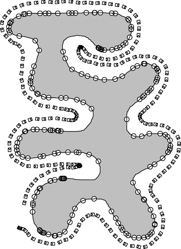
Figure 4.10: Trajectory for Simulations with a relatively simple obstacle.

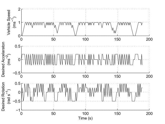
Figure 4.11: Control time history for simulations with a relatively simple obstacle.

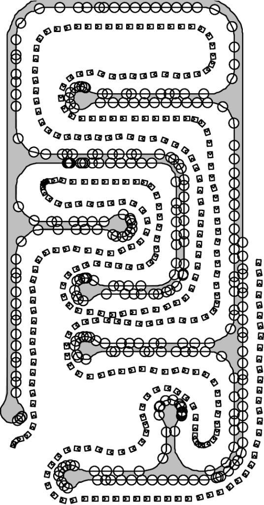
Figure 4.12: Trajectory for simulations with a more complex obstacle.

Figure 4.13: Control time history for simulations with a more complex obstacle.

When a target point was defined (for the simulations shown in Figs. 4.14 and 4.15), the vehicle was able to efficiently converge to the target. A random decision was made after the two straight segments present, as there were insufficient obstacle detections to guarantee the position of the obstacle boundary. This means a different value would lead to a different realization of the trajectory, however it would still converge to the target. As stated previously, high level decision making would provide a better alternative to this simplified method.

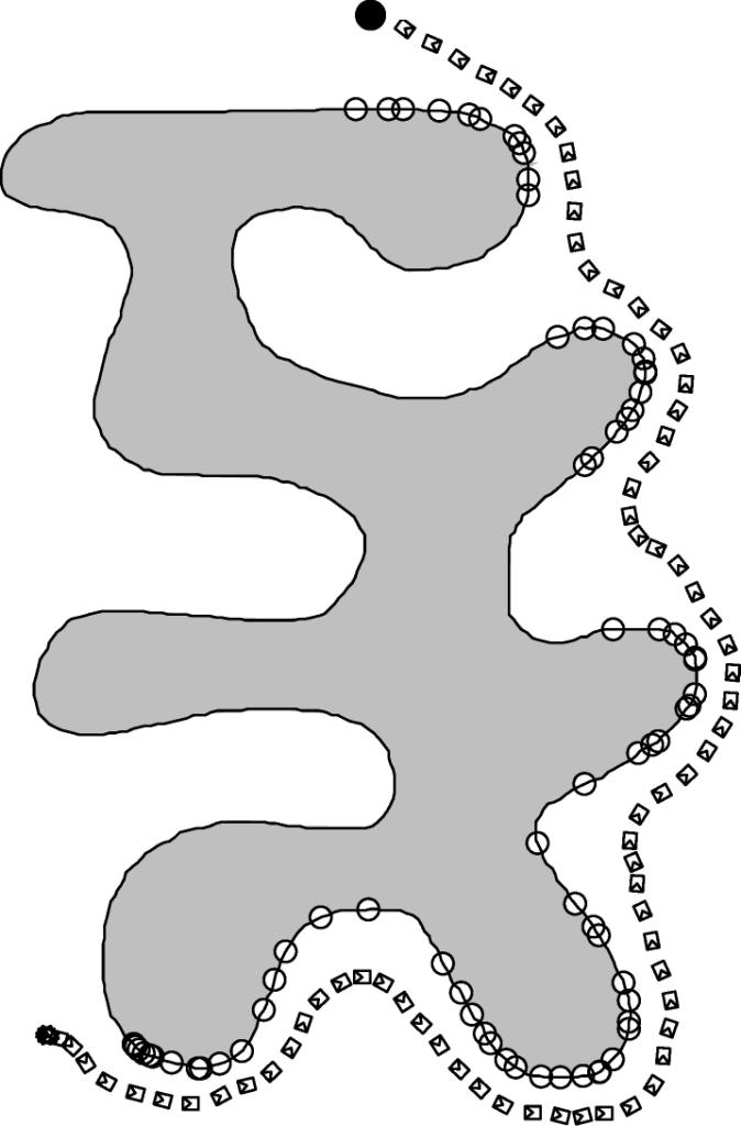
Figure 4.14: Trajectory for simulations with target convergence.

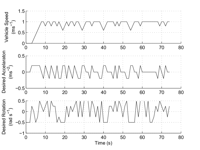
Figure 4.15: Control time history for simulations with target convergence.

For Figs. 4.16 and 4.17, during simulation the obstacle moves to the right at a speed of $0.1ms^{-1}$ (the trajectory is drawn from both the obstacle’s and the vehicle’s reference frame). The vehicle was given the precise velocity vector of the obstacle, which negated the need to implement an obstacle tracking algorithm. The effect of the moving obstacle can be observed especially around the points where the vehicle is moving slowly around corners - the motion appears to be sideways in the moving frame. While the only assumption on obstacle velocity was that it was below the maximum vehicle velocity, higher obstacles velocities within this limit were observed to reduce the likelihood of successful navigation (through safety was not affected).

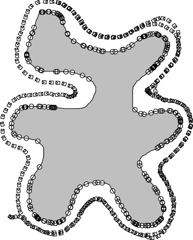
Figure 4.16: Simulations where the obstacle is moving; (a) Obstacle’s reference frame; (b) Vehicle’s reference frame.

Figure 4.17: Control time history for simulations where the obstacle is moving.

The proposed control law (PCL) was also compared with an existing boundary following control law from the literature [110], which is referred to as the alternate control law (ACL). The method of generating target points for the ACL (called ‘instant goals’) is similar, but not identical, to the method employed by the PCL. However, the key difference is that the ACL uses a potential field type term to maintain the required distance from the boundary, whereas the PCL employs path planning. The ACL also assumes a velocity controlled holonomic vehicle model, and to highlight the advantage of the PCL, the ACL was applied to the unicycle model. To do this, the maximal control inputs tending the vehicle’s heading and speed to the output of the ACL were implemented. The tunable parameter $\xi$ was taken to be 20, in-line with the recommendations of the method, and $V_{opt}$ was taken to be the same as $v_{max}$ from the PCL.

Figure 4.18: Comparison which an alternate control law from the literature; (a) PCL; (b) ACL.

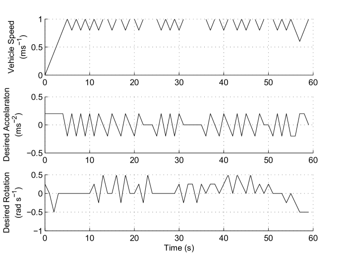
Figure 4.19: Control time history for PCL.

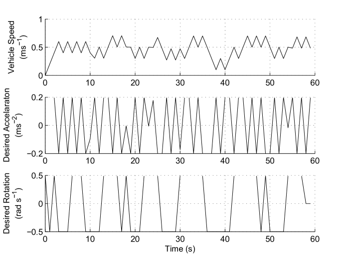
Figure 4.20: Control time history for ACL.

The results can be seen in Fig. 4.18, with the control time histories shown in Figs. 4.19 and 4.20. It can be seen the ACL is slower, and is affected by oscillation. The speed is set by a fixed computation and is not directly adjustable. The oscillation is presumably caused by the extra kinematics, which are not allowed for by the ACL.

4.6 Experiments

Experiments were performed with a Pioneer P3-DX mobile robot to show real-time applicability of this system (see Fig. 4.21). A SICK LMS-200 laser range-finding device was used to detect obstacles in a vicinity of the vehicle. This device has a nominal accuracy of $15mm$ along each detection ray (however this may be significantly degraded in real world circumstances [282]). Each measurement was used directly as a separate detection ray in the sensor model described by Assumption 4.1.1, after being cropped to be less than $R_{max}$. The standard on-board PC for a P3-DX was used, which is equipped with a 1.6 GHz Pentium processor.

The robot is equipped with the ARIA library (version 2.7.4) which provides commands to control the motor drives. At each control update, the desired translational acceleration and turning rate of the ARIA interface were set to match the outputs generated by the navigation algorithm. Note the recovery scheme was not implemented as it was never requested by the navigation algorithm (this may require additional feedback control to stabilize the position of the vehicle). The navigation calculation and robot control update was carried out at $0.1s$ sampling periods, however the sampling period for generating trajectories was increased to $1.0s$ to reduce computational load (this does not affect the properties of the navigation law). The initial $C_{end}$ was taken to be the nearest detected point. The values of the parameters used in the experiments are listed in Table 6.2. The physical parameters of the vehicles result from conservative estimates, whereas exact identification was not carried out. The obstacle was assumed to be stationary.

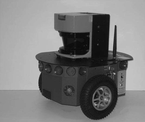
Figure 4.21: Pioneer P3-DX mobile vehicle used for testing.

$u_{\theta,max}$	$0.8rads^{-1}$
$u_{v,nom}$	$0.1ms^{-2}$
$v_{max}$	$0.4ms^{-1}$

$d_{ob}$	$0.15m$
$d_{rad}$	$0.3m$
$R_{max}$	$4m$
$N_{r}$	$90$ (semicircular)

Table 4.2: Experimental parameters for boundary-following controller.

Note that while the algorithm specification assumes a full circular field of view, the sensor used can only sense the half plane in front of the vehicle. Through not covered by the analysis, it seems logical to continue to enforce the same constraints. Conveniently, the constraint that requires the visibility of the obstacle to be maintained may compensate for the deficiency; however, because of disturbance, there is a possibility (however unlikely) for the vehicle to lose sight of the obstacle while navigating certain types of corner. However, an experimental design that produced these conditions was unable to be found.

In Fig. 4.22, the obtained closed loop trajectory recorded using a camera is presented, where the trails are plotted by manually marking the video sequence. It can be seen that the vehicle performed as expected, making reasonably consistent loops along the boundary.

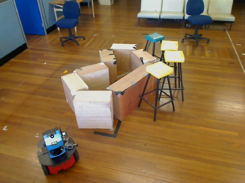
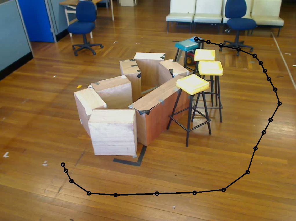
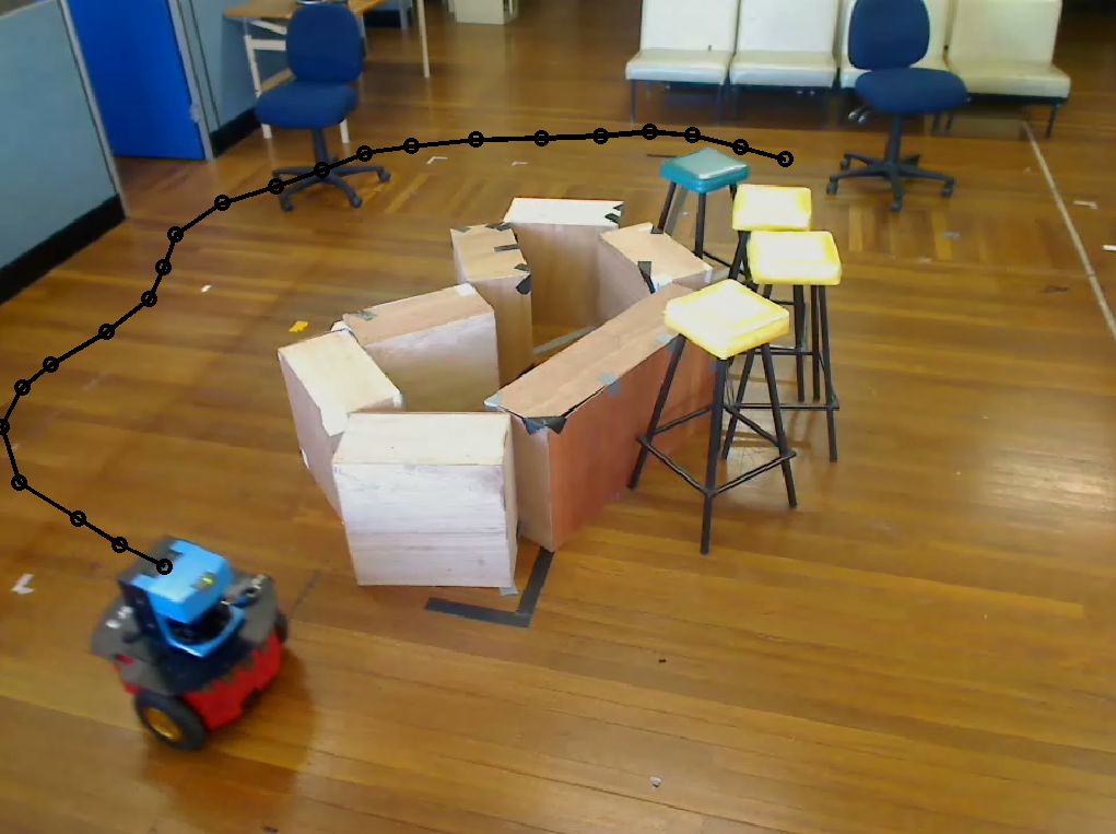
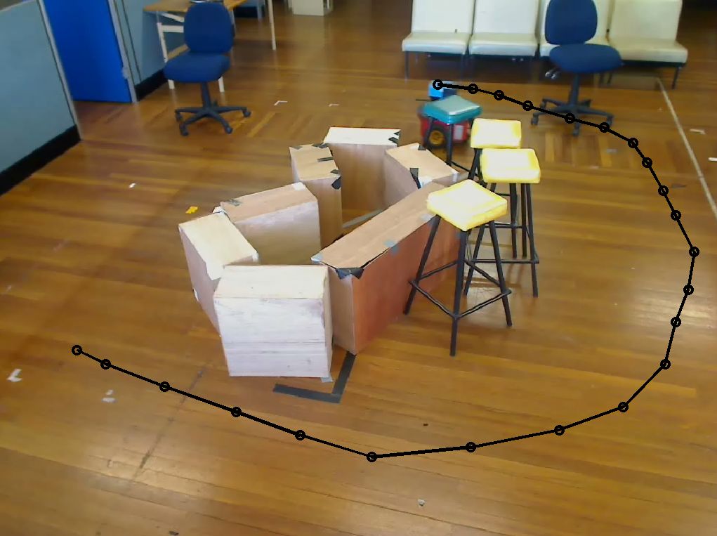
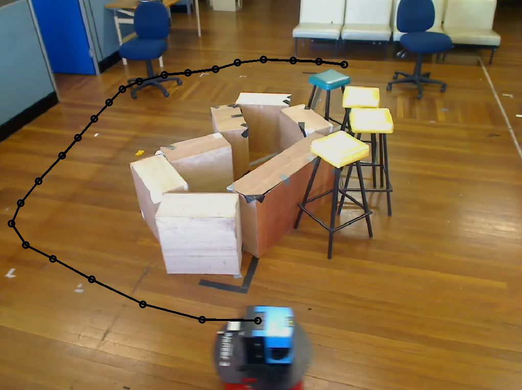
Figure 4.22: Sequence of images showing the experiment.

In Fig. 4.23 the estimated global heading recorded by odometry is shown, and it may be seen that the vehicle performs just over two complete loops around the obstacle. In Fig. 4.24 the minimum distance to the obstacle was always greater than 0.43 $m$, which is congruent with the chosen $d_{tar}$ (0.45 $m$). In Fig. 4.25 the vehicle velocity mostly stayed near the maximum (nominal) velocity (0.4 $ms^{-1}$), except for some brief reductions in speed. These reductions in speed are most likely caused by the maximum (nominal) speed being too fast to successfully navigate certain segments of the obstacle. In Fig. 4.26 the distance to the target point was always well over 1.3 $m$, which is expected.

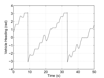
Figure 4.23: Evolution of the heading of the robot over the experiment.

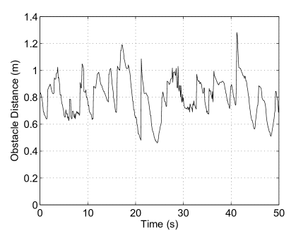
Figure 4.24: Minimum distance measured by the LiDAR sensor over the course of the experiment.

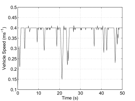
Figure 4.25: Speed of the robot over the course of the experiment.

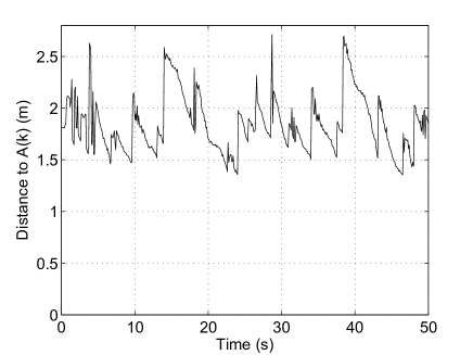
Figure 4.26: Distance to the target point $A(k)$ over the course of the experiment.

Future work may look at performing experiments with target convergence and with moving obstacles; however these tests indicate proof of concept for the basic control law.

4.7 Summary

In this chapter a method for navigating a vehicle along an obstacle boundary was proposed when local information from a range finding device is available. The MPC-type approach proposed here is able to plan a trajectory towards the edge of the points known to be a solid obstacle boundary. This allows the obstacle offset and vehicle speed to change appropriately to the obstacle. It was shown that every point on a finite obstacle boundary will have a nearby detection within a finite time. Possible extensions to target convergence and moving obstacles were presented. Computer simulations and real world testing confirm the methods validity.

Chapter 5 Collision Avoidance with Multiple Vehicles

In this chapter, the problem of decentralized collision avoidance of multiple vehicles operating in a common workspace is considered. Briefly, this is accomplished by introducing constraints to the trajectory selection process which are able to maintain non-interfering trajectories despite communication delay. This is offered as an alternative to the methods of multiplexed MPC and coherency objectives, which were discussed in Chapt. 2.

Here, a MPC type method is proposed that requires only a single communication exchange per control update and addresses the issue of communication delay. The proposed approach does not employ imposing an artificial and auxiliary coherence objective, and may be suited to real-time implementations, while retaining robustness properties.

The body of this chapter is organized as follows. In Sec. 5.1, the problem statement is explicitly defined and the vehicle model is given; in Sec. 5.2, the structure of the navigation system is presented. Simulation results with a perfect unicycle model are in Sec. 5.3; Experiments are in Sec. 5.4. Finally, Sec. 5.5 offers brief conclusions.

5.1 Problem Statement

In this chapter, $N_{h}$ autonomous vehicles traveling in a plane are considered, each of which is associated with a steady point target $T_{i},i\in[1:N_{h}]$. As before, the plane contains a set of unknown, untransversable, static, and closed obstacles $D_{j}\not\ni T_{i},j\in[1:n]$. As in Chapt. 3, the objective is to design a navigation law that drives every vehicle towards the assigned target through the obstacle-free part of the plane $F:=\mathbb{R}^{2}\setminus D$, where $D:=D_{1}\cup\ldots\cup D_{n}$. As before the distance from the vehicle to every obstacle and other vehicles should constantly exceed the given safety margin $d_{sfe}$. Thus it follows the vehicle’s physical radius would be less than $\frac{1}{2}d_{sfe}$.

In this chapter, only the unicycle model is considered for brevity, through these results could easily be extended to the holonomic model. As in Chapt. 3, it is assumed that the vehicle has knowledge of an arbitrary subset of the obstacle free part of the plane, $F_{vis,i}(k)\subset F$; the vehicle has knowledge of its current state $\mathscr{S}$; and the vehicle has access to the position of its target $T_{i}$.

Figure 5.1: Scenario containing several vehicles and static obstacles.

It is assumed the vehicles have capability of communication with nearby companions – every vehicle is able to broadcast to the other vehicles within a given radius $C$. Any communication delay is assumed to be less than the time step, so that any data transmitted at time step $k$ from one vehicle is available at time $k+1$ at all vehicles within the communication radius.

The vehicles need not be identical – the model parameters and the characteristics of the sensed area $F_{vis,i}(k)$ may depend on the vehicle index $i$. However it is assumed that the communication radius $C$ is the same for all vehicles (in other words, the communication graph is undirected). Furthermore, it is assumed that each vehicle has knowledge of all the fixed parameters of other vehicles inside the communication radius, by broadcast or otherwise.

It is required that the sampling times of each vehicle are synchronized, however communication based algorithms are available for the task of synchronization [115, 323, 365].

Remark 5.1.1

There is a limit to the number of agents that lie within the communication range of a particular vehicle, owing to the constraint on the minimum distance between the vehicles. This entails a bound on the maximum communication burden on each vehicle caused by scaling the number of vehicles.

Finally, as in Chapt. 3, it is assumed that the vehicles are subjected to external disturbances. To highlight the major points by dropping secondary and standard technical details, perfect measurement of the vehicle state is assumed. At the same time, bounded state estimation and obstacle measurement errors can be taken into account in a similar way, which point of view transforms estimation error into disturbance.

5.2 Navigation System Architecture

As in Chapt. 3, navigation is based on generating probational trajectories over the relatively short planning horizon $[k,(k+\tau)]$ at every time step $k$. Probational trajectory is nominal and is specified by a finite sequence of way-points, which satisfy the constraints of the nominal model. As before, probational trajectories necessarily halt at the terminal planning time. When necessary, the trajectory can be being prolonged arbitrarily by the ‘stay still’ maneuver.

At any sampling time $k$, every vehicle broadcasts its current state $\mathscr{S}$ and probational trajectory, which data arrive at the vehicles in the communication range one time step later. To avoid collisions with the companions, the vehicle also attempts to reconstruct their current probational trajectories, starting with reconstruction of the planned ones. However, the latter start at the current states of the companions, which are unknown to the vehicle at hand. So the vehicle first estimates these states on the basis of the received states at the previous time step (the estimate may differ from the actual state because of the disturbances). After this the vehicle copycats generation of the planned trajectories for every vehicle in the communication range, with substituting the estimate in place of the true state in doing so. This gives rise to the set of presumable planned trajectories.

5.2.1 Overview

The Trajectory Tracking Module (TTM) is identical to the presentation in Chapt. 3. However, the Trajectory Planning Module (TPM) is similar to the process employed in Chapt. 3. Every vehicle iteratively executes the following steps; in this enumeration, only Steps S.2 and S.5 are different:

1. Generation of a finite set $\mathscr{P}$ of planned trajectories, each starting at the current vehicle state $\mathscr{S}$.

2. Refinement of $\boldsymbol{\mathscr{P}}$ to only mutually feasible trajectories (see Sec. 5.2.3).

3. Selection of a trajectory from $\mathscr{P}$:

   • If $\mathscr{P}$ is empty, the probational trajectory is inherited from the previous time step (with a proper time shift).

   • Otherwise, the probational trajectory is updated by choosing an element of $\mathscr{P}$ minimizing some cost function (see Sec. 5.2.4).

4. Transmission of the chosen probational trajectory $\boldsymbol{s}^{*}(j|k)$ and the current state $\boldsymbol{\mathscr{S}}$ to all vehicles within the communication radius $\boldsymbol{C}$.

5. $k:=k+1$ and go to S.1.

This navigation process is executed co-currently in each vehicle. The overall architecture of the navigation system is illustrated in Fig. 5.2. Step S.2 is solely based on the currently observed part of the environment and data received from and sent to other vehicles in communication range since time step $k-1$. This step involves construction of the set of presumable planned trajectories for all vehicles in the communication range.

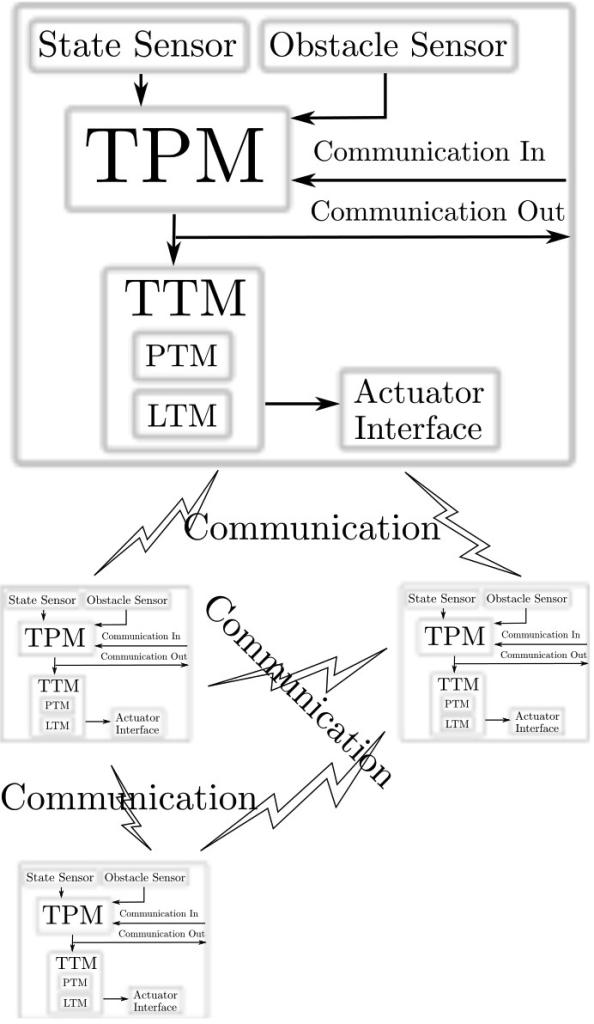
Figure 5.2: The overall architecture of the navigation system.

The upper index ^∗ is used to mark variables associated with the planned trajectories; this index is discarded to emphasize that the concerned trajectory is in fact probational; the hat $\widehat{\{\}}\vphantom{\}}^{\ast}$ is added to signal that a presumable planned trajectory is concerned. These variables depend on two arguments $(j|k)$, where $k$ is the time instant when the trajectory is generated, and $j\geq 0$ is the number of time steps into the future: the related value concerns the state at time $k+j$. Whenever a certain vehicle is considered, the lower index $\{\}_{i}$ refers to other vehicles within the communication range $C$, whereas its absence indicates reference to the vehicle at hand.

5.2.2 Safety Margins

To ensure collision avoidance, as before TPM respects more conservative safety margins than $d_{sfe}$. They take into account deviations from the probational trajectory caused by disturbances and are based on estimation of these mismatches.

Recall $d_{trk}$ is the maximum deviation between the vehicles actual state and the nominal state predicted by the probational trajectory. To simplify notations, it is assumed that $d_{trk}$ is the same for all vehicles; however the navigation scheme is still feasible if this quantity varies between them.

The following more conservative safety margins account for not only disturbances but also the use of time sampling in measurements of relative distances:

$$d_{tar}:=d_{sfe}+\frac{v_{max}}{2}+d_{trk},\qquad d_{mut}:=d_{sfe}+2\left[\frac{v_{max}}{2}+d_{trk}\right].$$ (5.1)

To illuminate their role, the following definition is introduced:

Definition 5.2.1

An ensemble of probational trajectories generated by all vehicles at a given time is said to be mutually feasible if the following claims hold:

1. The trajectory is feasible, i.e. the distance from any way-point to any static obstacle exceeds $d_{tar}$ for any trajectory;

2. For any two trajectories, the distance between any two matching way-points exceeds $d_{mut}$.

The motivation behind this definition is illuminated by the following:

Lemma 5.2.1

Let an ensemble of probational trajectories adopted for use at time step $k-1$ be mutually feasible. Then despite of the external disturbances, the vehicles do not collide with the static obstacles and each other on time interval $[k-1,k]$ and, moreover, respect the required safety margin $d_{sfe}$.

Proof

The static obstacle case follows from Lemma 3.2.1. For any pair of vehicles, the distance between the concerned way-points exceeds $d_{mut}$. So the the distance between the real positions at time $t$ is no less than $d_{mut}-2[\frac{v_{max}}{2}+d_{trk}]=d_{sfe}$. $\quad\bullet$

5.2.3 Trajectory Constraints

Refinement is prefaced by the following computations, which are carried out at the vehicle at hand for every vehicle $i$ that was within the communication range at the previous time step $k-1$:

• The nominal motion equations are integrated for vehicle $i$ from $k-1$ to $k$ with the initial data $\mathscr{S}_{i}(k-1)$ and controls $\mathscr{U}^{\ast}(0|k-1)$ to acquire the estimated current state $\widehat{\mathscr{S}}_{i}(k)$;

• The procedure from Sec. 3.2.3 is carried out for the $i$th vehicle, with the true current state $\mathscr{S}_{i}(k)$ replaced by the estimated one $\widehat{\mathscr{S}_{i}}(k)$.

This procedure is summarized in Fig. 5.3 and results in the set $\widehat{\mathscr{P}}_{i}$ of presumable planned trajectories of the $i$th vehicle.

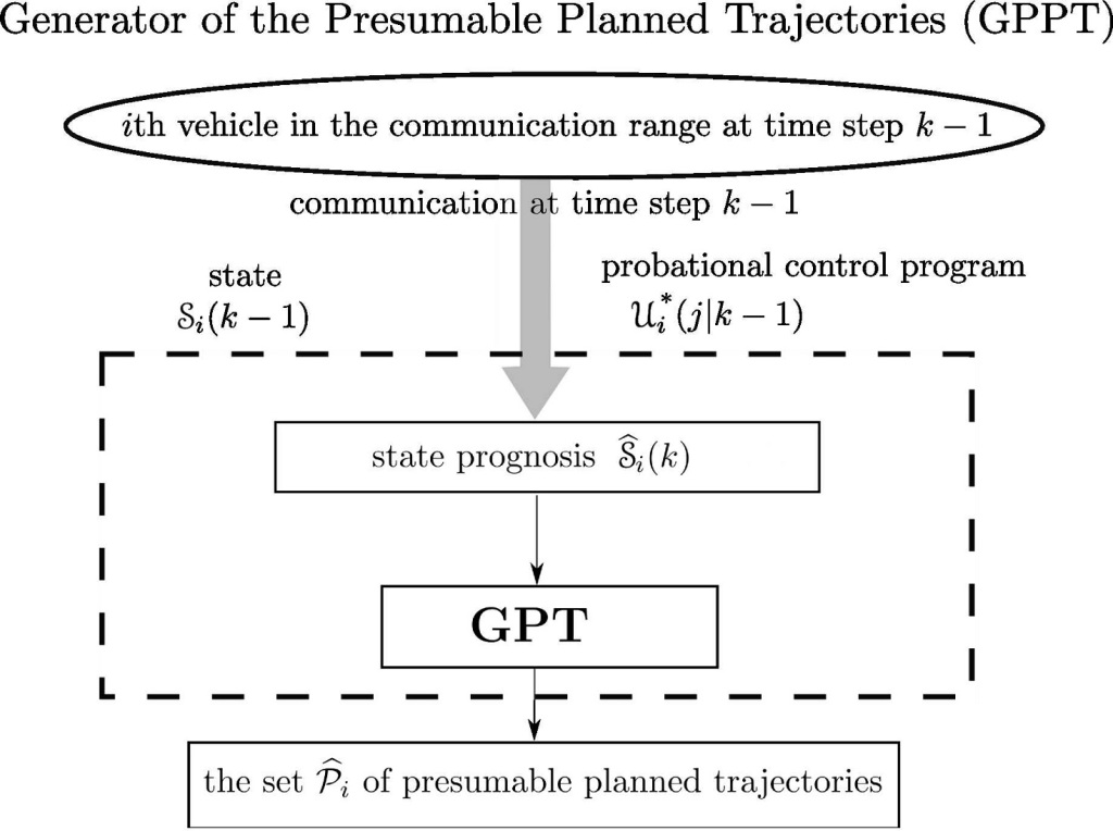
Figure 5.3: Generator of the planned trajectories.

To proceed, the following estimates are introduced:

• $\Delta_{osd}$ – an upper bound on the deviation over the single time step between the nominal and real state $\mathscr{S}$ of the vehicle driven by the TTM along the probational trajectory in the face of disturbances;

• $d_{\tau}$ – an upper bound on the translational deviation between two nominal trajectories over the entire planning horizon of duration $\tau$, provided that the difference between their initial states does not exceed $\Delta_{osd}$ and the both follow common speed and turning patterns selected by the trajectory generation rule from Sec. 3.2.3.

The constant $\Delta_{osd}$ is similar to $d_{trk}$; its computation is discussed in Sec. 3.2.4. $\Delta_{osd}$ and $d_{\tau}$ are illustrated in Fig. 5.4.

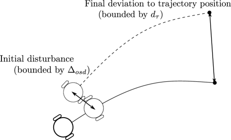
Figure 5.4: Effect of disturbance over a single time-step.

Given $\Delta_{osd}$, the bound $d_{\tau}$ can be easily computed based on the vehicle model. More or less conservative bounds can be used, up to the tight bounds based on computer-aided calculation of the reachable sets. However the experimental results show that even conservative estimates are able to entail good performance. Partly in view of this and partly due to the fact that computation of conservative bounds is elementary, the related details are omitted.

Note that Remark 3.2.1 is evidently extended on $\Delta_{osd}$ and $d_{\tau}$. The following remark is immediate from the foregoing and partly elucidates the role of $d_{\tau}$:

Remark 5.2.1

The mismatch $\max_{j=0,\ldots,\tau}$ $\lVert\boldsymbol{s}_{i}(j|k)$ $-$ $\widehat{\boldsymbol{s}}\vphantom{\boldsymbol{s}}_{i}(j|k)\rVert$ between the presumable planned trajectory and the true planned trajectory does not exceed $d_{\tau}$.

In order to ensure that the probational trajectories are mutually feasible, the set of planned trajectories is subjected to a series of refinements. First, the vehicle at hand refines the generated set of presumable planned trajectories $\{\widehat{\boldsymbol{s}}\vphantom{\boldsymbol{s}}_{i}^{\;\ast}(j|k),\ldots\}_{j}$ of any other vehicle $i$ that was in the communication range at the previous time step $k-1$. Specifically, it discounts any presumable trajectory that interferes with the true probational trajectory of the vehicle at hand $\{\boldsymbol{s}(j|k-1),\ldots\}_{j}$ selected at the previous time step $k-1$, i.e., such that:

$$\lVert\widehat{\boldsymbol{s}}\vphantom{\boldsymbol{s}}_{i}^{\;\ast}(j|k)-\boldsymbol{s}(j+1|k-1)\rVert\leq d_{mut}-d_{\tau}\quad\text{for some}\quad j.$$ (5.2)

This operation is summarized in Fig. 5.5 and gives rise to the set of the refined presumable planned trajectories $\widetilde{\mathscr{P}}_{i}$ of the $i$th vehicle.

Figure 5.5: Generator of the presumable planned trajectories.

After this, the vehicle at hand refines its own set of planned trajectories by successively discounting those interfering with:

1. Static obstacles, such that:

   $$\lVert\boldsymbol{s}^{*}(j|k)-x\rVert<d_{tar}\quad\text{for some}\quad x\in D,\quad\text{ and}\quad j$$ (5.3)

2. Probational trajectories of other vehicles received from them within the time interval $[k-1,k]$, such that:

   $$\lVert\boldsymbol{s}^{*}(j|k)-\boldsymbol{s}_{i}(j+1|k-1)\rVert<d_{mut}\quad\text{for some}\;j$$ (5.4)

3. Any refined presumable planned trajectory of any other vehicle $i$ that was in the communication range of the vehicle at hand at the previous time step $k-1$:

   $$\lVert\boldsymbol{s}^{*}(j|k)-\widehat{\boldsymbol{s}}\vphantom{\boldsymbol{s}}_{i}^{\;\ast}(j|k)\rVert<d_{mut}+d_{\tau}\;\text{for some}\;j\;\text{and}\;\{\widehat{\boldsymbol{s}}\vphantom{\boldsymbol{s}}_{i}^{\;\ast}(j|k),\ldots\}\in\widetilde{\mathscr{P}}_{i}.$$ (5.5)

As stated previously, if this refinement sweeps away all trajectories, the probational trajectory from the previous time step can be used. This leads to the following:

Lemma 5.2.2

The proposed refinement procedure does ensure that the probational trajectories generated at time step $k$ are mutually feasible provided that the probational trajectories were mutually feasible at the previous time step $k-1$.

Proof

Let us interpret vehicles $j$ and $i$ as the ‘vehicle at hand’ and the ‘other vehicle’, respectively; according to the adopted notation, this means the index $j$ may be dropped everywhere. Also note the probational trajectories were selected from the set of planned trajectories, i.e. $\boldsymbol{s}(\cdot|k)=\boldsymbol{s}^{\ast}(\cdot|k),\boldsymbol{s}_{i}(\cdot|k)=\boldsymbol{s}_{i}^{\ast}(\cdot|k)$.

The trajectory $\boldsymbol{s}_{i}^{\ast}(\cdot|k)$ has passed the test from r.2) at the vehicle $i$ and so does not interfere with the trajectory transmitted from the vehicle at hand at time step $k-1$, such that $\lVert\boldsymbol{s}_{i}^{\ast}(r|k)-\boldsymbol{s}(r+1|k-1)\rVert>d_{mut}\;\forall r$. For the related presumable planned trajectory, it follows:

$$\lVert\widehat{\boldsymbol{s}}\vphantom{\boldsymbol{s}}_{i}^{\ast}(r|k)-\boldsymbol{s}(r+1|k-1)\rVert\geq\lVert\boldsymbol{s}_{i}^{\ast}(r|k)-\boldsymbol{s}(r+1|k-1)\rVert\\ -\underbrace{\lVert\widehat{\boldsymbol{s}}\vphantom{\boldsymbol{s}}_{i}^{\ast}(r|k)-\boldsymbol{s}_{i}^{\ast}(r|k)\rVert}_{\leq d_{\tau}\;\text{by Remark~{}\ref{rem.mismatch}}}\geq d_{mut}-d_{\tau}.$$ (5.6)

So this trajectory was among those against which $\boldsymbol{s}^{\ast}(\cdot|k)$ was tested in correspondence with Eq.(5.5). Since $\boldsymbol{s}^{\ast}(\cdot|k)$ has survived the refinement procedure, this test was passed:

$$\lVert\boldsymbol{s}^{*}(r|k)-\widehat{\boldsymbol{s}}\vphantom{\boldsymbol{s}}_{i}^{\;\ast}(r|k)\rVert>d_{mut}+d_{\tau}\qquad\forall r.$$

The proof is completed by invoking the under-braced inequality from Eq.(5.6):

$$\lVert\boldsymbol{s}(r|k)-\boldsymbol{s}_{i}(r|k)\rVert=\lVert\boldsymbol{s}^{\ast}(r|k)-\boldsymbol{s}_{i}^{\ast}(r|k)\rVert\geq\lVert\boldsymbol{s}^{\ast}(r|k)-\widehat{\boldsymbol{s}}\vphantom{\boldsymbol{s}}_{i}^{\ast}(r|k)\rVert\\ -\lVert\boldsymbol{s}_{i}^{*}(r|k)-\widehat{\boldsymbol{s}}\vphantom{\boldsymbol{s}}_{i}^{\;\ast}(r|k)\rVert\geq d_{mut}+d_{\tau}-d_{\tau}=d_{mut}.$$

This completes the proof. $\quad\bullet$

By retracing the arguments of the first part of the proof and invoking Remark 5.2.2, the following statement can be made:

Remark 5.2.2

It is assumed that initially there are no vehicles in communication range of each other and every vehicle is far enough from the static obstacles so that at least one planned trajectory survives r.1). Then the generated set of probational trajectories is well-defined and mutually feasible, so it also follows that this set remains mutually feasible in subsequent time steps.

The overall performance of the entire navigation system is addressed in the following:

Proposition 5.2.1

Let every vehicle be driven by the proposed navigation law. Then the vehicles do not collide with the static obstacles and each other and, moreover, respect the required safety margin $d_{sfe}$.

Proof

By Lemma 5.2.2 and Remark 5.2.2, the ensemble of probational trajectories adopted for use at any step is mutually feasible. Lemma 5.2.1 completes the proof. $\quad\bullet$

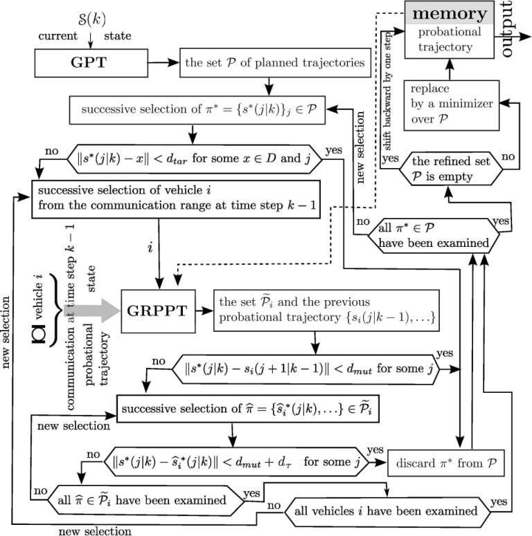
Figure 5.6: Trajectory Planning Module.

Input: The current state of the vehicle: $\mathscr{S}(k)\equiv\langle\boldsymbol{s}(k),\theta(k),v(k)\rangle$

The probational trajectory that is the previous output of the algorithm: $\{\boldsymbol{s}^{*}(j|k-1),\ldots\}$

The trajectories received from other vehicles: $\{\boldsymbol{s}_{i}^{*}(j|k-1),\ldots\}$

The currently sensed obstacle set $F_{vis,i}(k)$

Output: Current probational trajectory: $\{\boldsymbol{s}^{*}(j|k),\ldots\}$

Process:

Generate the set of planned trajectories $\mathscr{P}$

Remove from $\mathscr{P}$ the trajectories that are closer than $d_{tar}$ to the currently sensed obstacle set

foreach Received trajectory $\{\boldsymbol{s}_{i}^{*}(j|k-1),\ldots\}$ do

       Remove from $\mathscr{P}$ the trajectories that are closer than $d_{mut}$ to $\boldsymbol{s}_{i}^{*}(j|k-1)$

       Generate the set of presumable planned trajectories $\widehat{\mathscr{P}}_{i}$ based on $\mathscr{S}^{\ast}(1|k-1)$

       Remove from $\widehat{\mathscr{P}}_{i}$ the trajectories that are closer than $d_{mut}-d_{\tau}$ to $\boldsymbol{s}^{*}(j|k-1)$

       Remove from $\mathscr{P}$ the trajectories that are closer than $d_{mut}+d_{\tau}$ to some trajectory in the remaining set $\widehat{\mathscr{P}}_{i}$

      

end foreach

if $\mathscr{P}=\emptyset$ then

       Reuse the trajectory from the previous time-step

end if

else

       Select a minimizer of Eq.(5.8) over $\mathscr{P}$

end if

Algorithm 1 Operation of TPM.

This operation is summarized in Fig. 5.6 and by the pseudo-code Algorithm 1. Note an upper bound on the total computation load is proportional to:

$$O(N_{v},N_{t},N_{p})=N_{v}\cdot N_{t}^{2}\cdot N_{p},\quad N_{t}=4\cdot\left\lceil\frac{\tau}{\Delta\Lambda}\right\rceil+2,\quad N_{p}\equiv\tau$$ (5.7)

where $N_{v}$ is the number of the vehicles in the communication range and $N_{t}$ is the number of planned trajectories. As for the communication load, only four reals are required to encode the state for communication, with extra two integers being needed to encode the index of the trajectory inside $\mathscr{P}$ and the progression along the trajectory.

Modulo slight extension, the proposed algorithm also displayed good resistance to packet dropouts, which are common in wireless communications [352]. The only trouble caused by a packet dropout is that the vehicle loses access to the state and probational trajectory of some ‘other’ vehicle at the previous time step and so is unable to carry out the proposed refinement procedure; see Sec. 5.2.3. This trouble can be easily overcome by employing the latest known data about the ‘other’ vehicle, which is brought by the last successful transmission. This however gives more conservative approximations of the true planned trajectories If this conservatism appears to be too large, trajectory tracking would be engaged. Thus it can be reasonably inferred that packet loss will reduce the system performance, though can hardly violate robustness.

The main advantage of the proposed approach is its ‘reactiveness’: collision avoidance only requires a single time step of latency for communication between vehicles before mutual action is taken.

5.2.4 Implementation Details

From the set of the planned trajectories surviving the refinement procedure, the final trajectory is selected to furnish the minimum of the cost functional:

$$J=\lVert\boldsymbol{s}^{*}(\tau|k)-T\rVert-\gamma_{0}\cdot v^{*}(1|k),$$ (5.8)

where $T$ is the target for this vehicle and $\gamma_{0}>0$ is a given weighting coefficient, which may depend on the vehicle. This minimization aims to align the vehicle with the target while preferring trajectories with faster initial planned speeds, and gave good results when implemented.

Simulations and experiments (see Secs. 5.3 and 5.4, respectively) have shown that the proposed navigation strategy does allow every vehicle to efficiently converge to its assigned target in most circumstances. Occasionally in scenarios with high vehicle densities, some deadlocks may be avoided by instructing the vehicles to rotate in place to present different initial states to the planner.

5.3 Simulations

Simulations were carried out in MATLAB with a perfect unicycle model, with parameters given in Table 5.1. TPM and TTM updates occurred at 1 Hz and 10 Hz, respectively. To examine the sensor noise implications, vehicle state measurements were corrupted by bounded, random, uniformly distributed zero mean errors. The magnitude of these was $0.1m$ for the translational position measurement and $0.02rad$ for the heading measurement. Acquisition of data about obstacles was modeled as rotation of the detection ray with the step of $0.157rad$, finding the distance to the obstacle reflection point, and interpolation of the reflection points by straight line segments. Once the vehicles were within $0.5m$ of their targets, the navigation task was assumed to be completed and so the navigation signals were set to zero.

$R_{sen}$	$4.0m$
$C$	$8.5m$
$d_{tar}$	$0.50m$
$v_{max}$	$1.1ms^{-1}$
$u_{\theta,max}$	$3.0rads^{-1}$
$u_{v,max}$	$0.30ms^{-2}$
$v_{nom}$	$1.0ms^{-1}$

$u_{\theta,nom}$	$1.0rads^{-1}$
$u_{v,nom}$	$0.20ms^{-2}$
$\Delta\Lambda$	$0.25$
$k_{0}$	$1$
$k_{1}$	$1$
$\gamma_{0}$	$1$
$\mu_{\varkappa}$	$0.9$

Table 5.1: Simulation parameters for multiple-vehicle controller.

The path tracking surfaces were taken to be:

$$\chi(z) =\text{\bf sgn}(z)\cdot\min\{0.50\cdot|z|,0.50\}$$

$$\underline{\varkappa}(z) =0.05+\min\{1.0\cdot|z|,0.70\varkappa_{\text{v}}\}$$

$$p(S,z) =\min\{\underline{\varkappa}(z)+1.0S,\varkappa_{\text{v}}\}$$

The obtained closed loop trajectories are displayed in Figs. 5.7, 5.8, and 5.9. In all cases when the noise was absent from the system, the inter vehicle distance was constantly monitored by the simulation, and was observed to never drop below $0.995m$. This confirms the theoretical results – any slight deacreases below $d_{tar}$ can be explained by effects such as limited computational accuracy of the computer. The vehicle-obstacle distance never dropped below $0.495m$, in harmony with the chosen value of $d_{tar}$. When the sensor noise was added, as in the simulations shown in Figs. 5.7 to 5.9, the minimum observed inter-vehicle distance was $0.6547m$. This can be treated as disturbance, and the desired inter-vehicle distance can be increased accordingly if this separation is too small. In every case, the vehicles successfully converged to the assigned targets, for example in Fig. 5.9 the time taken for all vehicles to reach their targets was $70s$.

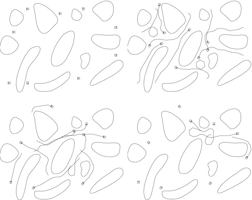
Figure 5.7: Simulations with nine vehicles in a complex scene.

Fig. 5.7 shows a collision avoidance maneuver for nine vehicles. This scenario may be encountered in an office, warehouse, factory or urban environment. The vehicles smoothly move around each other and adjust their speeds to prevent collisions. When a vehicle slows down its turning radius decreases, thus allowing sharper turns to be made (any of the points on the trajectory where the curvature is small would have been carried out at less than full speed). In addition, an interesting phenonemon was ‘wheeling’, where vehicles would move in a full circle, presumably to dealy its entry into an adjacent area.

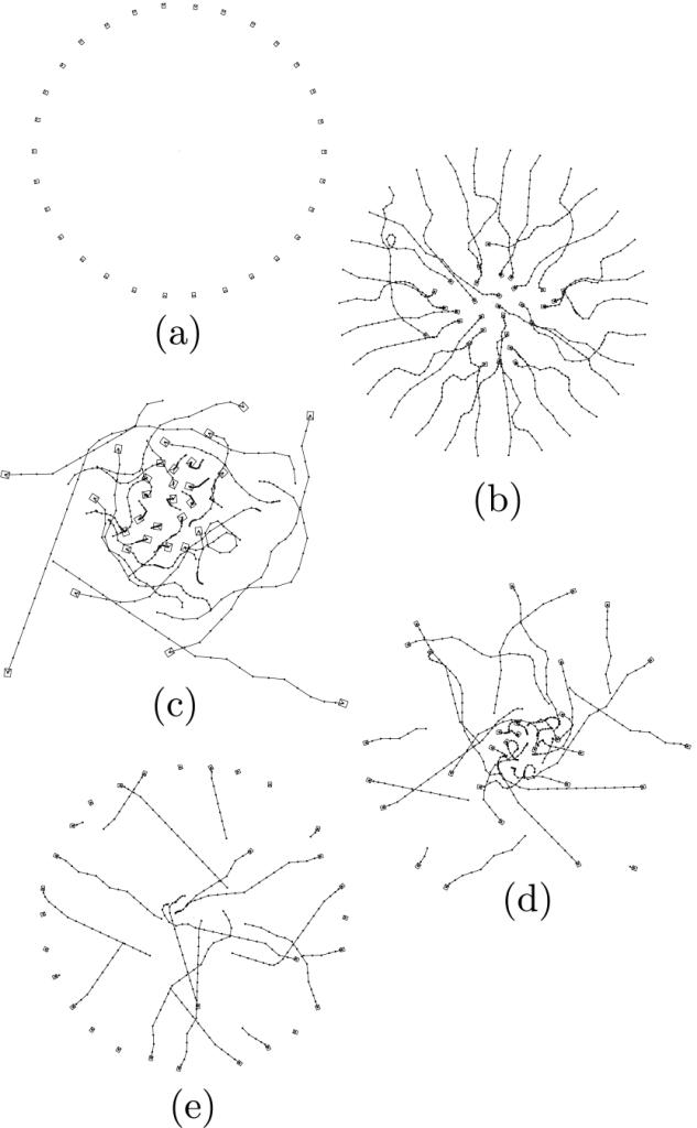
Figure 5.8: Simulations with thirty vehicles in an open scene.

Fig. 5.8 represents an obstacle free environment where thirty vehicles are initially aligned around the edge of a circle; every vehicle must exchange positions with the vehicle on the opposite side of the circle. Similar scenarios may be found in the literature [342]. While the motion looks like relatively chaotic, all vehicles still converged to the desired locations. At some points, some vehicles were stationary, and performing the rotation maneuver allows to find a trajectory after a short delay.

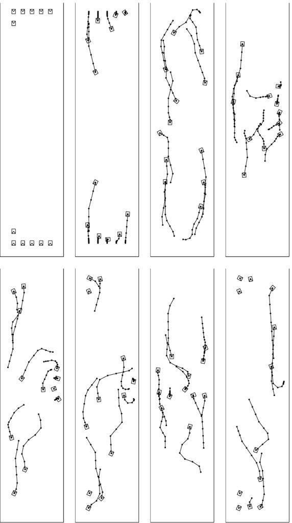
Figure 5.9: Simulations with twelve vehicles in a constrained environment.

Fig. 5.9 shows the results with twelve vehicles in a constrained environment. This experiment highlights that in complex situations higher order planning is useful to generate efficient solutions. However even in this situation, the vehicles were all able to progress towards their respective targets. Most importantly, collisions were always avoided.

Figure 5.10: Computation time relative to the number of vehicles present.

Fig. 5.10 shows the computation time of each execution of the algorithm on each vehicle on a 3 GHz Desktop PC. The maximum CPU time was under $50ms$ per vehicle per control update, even for thirty vehicles, which implies that the proposed approach is suitable for real time implementation.

Comparisons

In order to compare the performance of the proposed algorithm with other types of collision avoidance controllers, simulations were also carried out with a potential field type method [52, 129]. Various elements from these papers were combined to produce a controller that solves a problem similar to ours. In doing so, the nearest point on the static obstacle was treated as a virtual vehicle, as in [52]. The overall navigation law is given by the following expression, loosely based on [129]:

$$\left[\begin{array}[]{c}v_{t}(t)\\ w_{t}(t)\end{array}\right]=A^{-1}(\theta)\cdot\left(-\frac{1}{2}\mbox{\boldmath$\nabla$}\gamma-\sum_{i}\mbox{\boldmath$\nabla$}V_{i}\right)$$

Here $\gamma$ is a navigation function accounting for the distance to the target, $V_{i}$ is a repulsion potential with respect to the $i$th companion vehicle, and $A(\theta)$ translates the control signals from the vehicle’s reference frame into the global one:

$$A(\theta)=\left[\begin{array}[]{c c}\cos(\theta)&-l\sin(\theta)\\ \sin(\theta)&l\cos(\theta)\end{array}\right]$$

$$V_{i}=\left\{\begin{array}[]{c c}\left(\frac{1}{\beta_{i}^{2}}-\frac{1}{d_{sep}^{2}}\right)^{2}&\beta_{i}\geq d_{sep}\\ 0&\beta_{i}<d_{sep}\end{array}\right\},$$

where $\beta_{i}$ is the distance to the $i$th vehicle. The control signals produced by the above formulas were subjected to saturation with regard to their maximally feasible levels $u_{\theta,nom}$ and $u_{v,nom}$.

The controls were updated with a sampling time of $0.1s$, and $d_{sep}:=4m,l:=1m$. The vehicle completed the task when entering the disk of the radius $5m$ centered at its target.

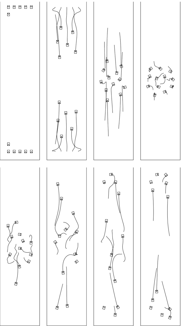
Figure 5.11: Simulations using a artificial potential field approach.

The potential field method (PFM) was tested in favorable circumstances where its well known disadvantages, like deadlocks caused by local minima due to, e.g., obstacle concavities, are unlikely to manifest themselves. The corresponding scene and results are shown in Fig. 5.11. Simulations showed that PFM took $96.7s$ to perform the maneuver, whereas the proposed navigation law (abbreviated to PCL in this discussion for clarity) took only $70s$, which is essentially quicker. At the same time, the total distance traveled by all vehicles is approximately the same for both methods: $280.52m$ for PFM and $282.40m$ for PCL. The minimum distance between the vehicles was $0.951m$ for PFM, whereas it was $1.001m$ for PCL. It is also worth noting that it was not difficult to find a simple alternative scenario where the above PFM failed to drive the vehicles to their assigned targets due to local minima, whereas PCL still succeeded.

5.4 Experiments

Experiments were carried out with two Pioneer P3-DX mobile robots to show real-time applicability of this system. As in Chapt. 4, a SICK LMS-200 laser range-finding device was used to detect obstacles in a vicinity of the vehicle. In order to localize the vehicles, they were launched from known starting positions and headings, and odometry feedback was used during the maneuver.

In the experiments presented here, this method resulted in a good enough performance, which is in harmony with [214], where the systematic error was reported to be under $1.5\%$ of the distance traveled. At each control update, as before the target translational acceleration and turning rate of the low level wheel controllers were set to match the results of the navigation algorithm. The laser detections in the circle of radius $d_{tar}$ around the estimated position of the other vehicle were excluded when computing the navigation approach to prevent detections of the other vehicle affecting the path computations. The values of the parameters used in the experiments are listed in Table 5.2.

$R_{sen}$	$4.0m$
$d_{tar}$	$0.30m$
$v_{max}$	$0.50ms^{-1}$
$u_{\theta,max}$	$0.80rads^{-1}$
$u_{v,max}$	$0.30ms^{-2}$
$v_{nom}$	$0.40ms^{-1}$
$u_{\theta,nom}$	$0.60rads^{-1}$

$u_{v,nom}$	$0.10ms^{-2}$
$\Delta\Lambda$	$0.50$
$k_{0}$	$1$
$k_{1}$	$1$
$\gamma_{vel}$	$1$
$\mu_{\varkappa}$	$0.9$

Table 5.2: Experimental parameters for multiple-vehicle controller.

The navigation scheme proposed in this chapter assumes decentralized communication. However for purely technical reasons, this decentralization was emulated on a common base station in the experiments so that the vehicles communicated with each other not directly but through this station. Communication was established via sending UDP packets over a 802.11g WLAN, with a checksum error detection scheme being employed [352]. A substantial rate of packet dropouts was observed, which according to Sec. 5.2.4 does not affect robustness but does affect performance. The event of packet dropout was handled similarly to the event where refinement of the set of planned trajectories results in the empty set – the previous probational trajectory remains in use. TTM and TPM were run at a common rate, the communication range covered the entire operational zone of the vehicles.

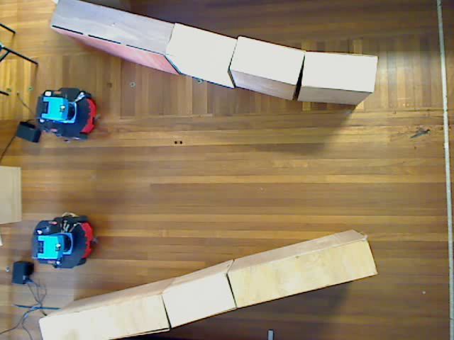
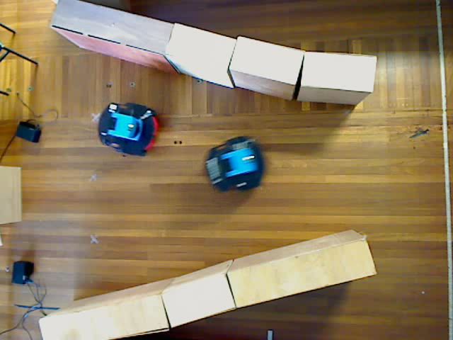
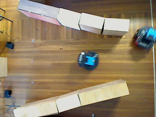
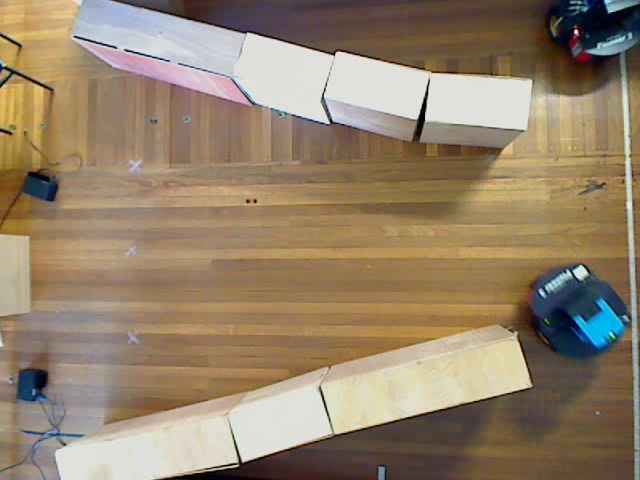
Figure 5.12: Sequence of images showing the experiment (parallel encounter).

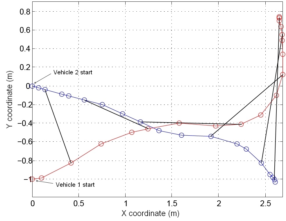
Figure 5.13: Trajectory for the experiment (parallel encounter).

In the first scenario demonstrated by Figs. 5.12 and 5.13, the vehicles are both trying to move through a gap which is only wide enough for one vehicle. The top vehicle allows the bottom vehicle to pass through a narrow region before moving into the gap itself.

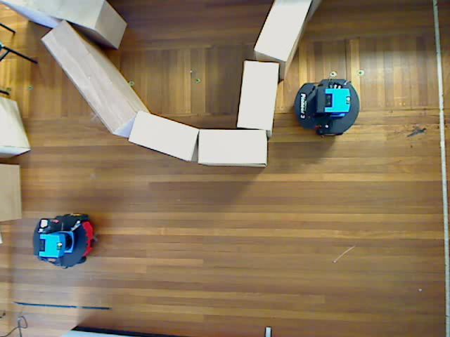
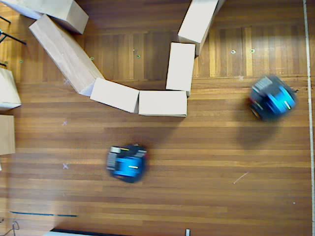
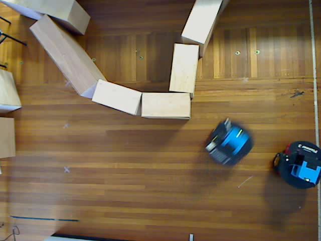
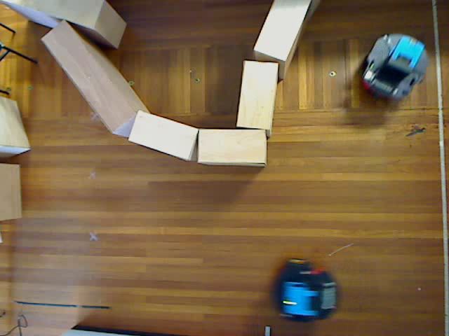
Figure 5.14: Sequence of images showing the experiment (head-on encounter).

Figure 5.15: Trajectory for the experiment (head-on encounter).

In the second scenario demonstrated by Figs. 5.14 and 5.15, the vehicles must pass each other while a static obstacle is present. The vehicle which begins on the left takes a longer path to prevent collision occurring.

5.5 Summary

In this chapter, a robust cooperative collision avoidance system is proposed, which is suitable for maintaining safety within a group of vehicles operating in unknown cluttered environments. By calculating a set of presumable planned trajectories for each vehicle within communication radius, it is possible to generate constraints which maintain mutually feasible trajectories, from which collision avoidance behaviour may be shown. The system was verified with simulations and tests on a pair of real wheeled mobile robots.

Chapter 6 Deadlock Avoidance

In recent times, many types of decentralized navigation strategies have been proposed to coordinate multiple vehicles and prevent collisions between them. In these situations, showing robust convergence to target is a equally important issue, however deadlock avoidance is generally a more complex and non-trivial subproblem which must be solved.

The approach presented in this chapter is motivated by the fact that, at least anecdotally, deadlocks most commonly occur in narrow corridors, i.e. where there is not enough room for vehicles to move past each other. Here, a hierarchy is enforced between the vehicles during encounters, which means the highest ranked vehicle will always have priority for transversing the corridor environment. This work is most applicable to unknown environments, where a map suitable for segmenting into a graph is not available. Also, no assumptions are made about the shape or geometry of the obstacle as was done in Chapt. 4. However to substitute this information, it will be assumed that a suitable navigation function exists.

As mentioned in the introduction, most research into deadlock free motion planning divides the workspace into some type of discrete graph, where the vehicle travels between nodes. This chapter is concerned with preventing deadlocks from a continuous state space perspective, where twin vehicle deadlocks may be classified into three categories; Type I deadlock may be resolved without the primary vehicle moving contrary to its objective; Type II deadlock requires the primary vehicle to temporarily move contrary to its objective; and finally, Type III deadlocks are impossible to solve. These categories are illustrated in Fig. 6.1.

Figure 6.1: Different categories of deadlock; (a) Type I; (b) Type II; (c) Type III.

In this chapter, almost all deadlocks are of the first kind. The second type are extremely rare, and would require use of the recovery scheme proposed in Sec. 6.2.3 to solve. The third type may only exist if the vehicles starting positions are inappropriate, and this is avoided by Assumption 6.1.3.

The body of this chapter is organized as follows. In Sec. 6.1 the problem statement is given; in Sec. 6.2 a new navigation system is proposed to avoid deadlocks. Simulations in a corridor environment are in Sec. 6.3; experiments are in Sec. 6.4. Finally, Sec. 6.5 offers brief conclusions.

6.1 Problem Statement

Two autonomous vehicles $\mathcal{R}_{1},\mathcal{R}_{2}$ are considered, which travel in a plane with maximum speed $v_{max}$, each of which is associated with a steady point target $T_{1},T_{2}$ respectively. $\mathcal{R}_{1}$ is designated the primary vehicle, which is given priority for navigation. As before the plane contains a set of untransversable, static, and closed obstacles $D_{j}\not\ni T_{i},j\in[1:n]$. The objective is to design a navigation law that drives every vehicle to their assigned targets in finite time through the obstacle-free part of the plane $\mathbb{R}^{2}\setminus D,D:=D_{1}\cup\ldots\cup D_{n}$. Moreover, the distance from the vehicle to every obstacle and other vehicle should constantly exceed the given safety margin $d_{sfe}$. As in previous chapters, a unit time-step is used for simplicity.

In this chapter, only the unicycle model is considered for brevity, through these results could easily be extended to the holonomic model. As in Chapt. 4, it is assumed that the system model is free from disturbance.

The trajectory structure and feasibility criteria employed in this chapter are identical to those in Chapt. 5. The main difference are minimum requirements on the sensed ares $F_{vis}(k)$. This generalized obstacle set characterization is described in the following assumption:

Assumption 6.1.1

The vehicle has perfect knowledge of the obstacle set within some distance $R_{con}<R_{sen}$ of the vehicle, such that:

$$F_{vis}(k)\supset\left\{\boldsymbol{x}\in F:\lVert\boldsymbol{x}-\boldsymbol{s}(k)\rVert\leq R_{con}\right\}$$ (6.1)

Communication assumptions are mostly identical to Chapt. 5, where vehicles have their control updates synchronized and experience unit communication delay. However in contrast to Chapt. 5, it is assumed that communication is always possible regardless of the distance between the vehicles.

In this chapter, the trajectory planning approach presented in Chapt. 3 must be slightly modified. This is because minimum requirements of the trajectory planner must be formulated in order to ensure convergent navigation. This involves allowing for sampling effects through a finite quantity $d_{pln}>0$ as follows:

Definition 6.1.1

A point is plannable if the minimum distance to the obstacle set $D$ exceeds $d_{tar}+d_{pln}$. The set of plannable points is denoted $G\subset F$.

The corresponding assumptions on the path planning system are located in Assumption 6.2.1. Any point not within $d_{pln}$ of the set of plannable points would be effectively be considered as non-feasible, through this is achieved without the consideration of the navigation system.

It is also assumed that a global navigation function (see e.g. [255]) is available and known to the vehicle:

Assumption 6.1.2

For any point $\boldsymbol{x}$, the vehicle has access to a navigation function $\mathscr{N}_{i}(\boldsymbol{x})$. If $\boldsymbol{x}\in G$, $\mathscr{N}_{i}(\boldsymbol{x})$ is defined as the minimum length of any curve intersecting both $\boldsymbol{x}$ and $T_{i}$, which is contained within the set of plannable points $G$. If such a curve does not exist, $\mathscr{N}_{i}(\boldsymbol{x}):=\infty$. If $\boldsymbol{x}\not\in G$, let $\acute{\boldsymbol{x}}:=\arg\min_{\acute{\boldsymbol{x}}\in G}\lVert\boldsymbol{x}-\acute{\boldsymbol{x}}\rVert$. Then $\mathscr{N}(\boldsymbol{x}):=\mathscr{N}(\acute{\boldsymbol{x}})+\lVert\boldsymbol{x}-\acute{\boldsymbol{x}}\rVert$.

It is assumed that the target $T_{i}$ is connected to the vehicle, such that the navigation function $\mathscr{N}$ is defined at both vehicles’ starting positions.

Based on the navigation function, the definition of a convergent trajectory can be introduced as follows:

Definition 6.1.2

A probational trajectory $s^{*}(j|k)$ is convergent if the navigation function $\mathscr{N}$ decreases by at least a decrement $d_{dec}$ from the initial point to any other point on the trajectory:

$$\max_{1\leq j\leq\tau}\mathscr{N}(\boldsymbol{s}^{*}(j|k))\leq\mathscr{N}(\boldsymbol{s}(k))-d_{dec}$$ (6.2)

It is permissible for only $\boldsymbol{s}^{*}(\tau|k)$ to be considered so long that the trajectory $\boldsymbol{s}^{*}(j|k)$ is followed to completion. In this case $\mathscr{N}(\boldsymbol{s}^{*}(\tau|k))\leq\mathscr{N}(\boldsymbol{s}(k))-d_{dec}$.

It is required that the given trajectory planning system is sufficiently complete, so that if there exists a convergent trajectory consisting of plannable points, the trajectory generation scheme will not fail to find at least one convergent, feasible trajectory.

Finally it is assumed that the targets and initial positions are sufficiently spaced from the obstacle, so that the other vehicle may successfully navigate around them:

Assumption 6.1.3

The points $T_{1}$, $T_{2}$,$\boldsymbol{s}_{1}(0)$, $\boldsymbol{s}_{2}(0)\in G$, and are spaced by at least $(2d_{tar}+2d_{pln})$ from $D$.

Remark 6.1.1

The use of a navigation function assumes the environment is previously known, and prevents the method from being classified as sensor based. It may be possible to replace the navigation function with a heuristic similar to the target convergence scheme in Chapts. 4 and 7.

6.2 Navigation System Architecture

The basic premise for deadlock avoidance is for the secondary vehicle to attempt to ensure the primary vehicle always has a valid trajectory to follow in the future. Additionally, the planning algorithm is extended with an additional trajectory shape. Also, a prescribed maneuver (the recovery scheme) is described for the vehicles to execute when all other possibilities are exhausted. This maneuver is guaranteed to result in at least a given progression along the navigation function of the primary vehicle.

Recall in Chapt. 3 only two possible longitudinal control patterns were considered – either the pattern $p_{+}:=(+--\ldots)$ or the pattern $p_{-}:=(---\ldots)$. In this chapter a third pattern $p_{s}$ is introduced, which is only considered when the vehicle is stationary ($v(k)=0$), where $p_{s}:=(0\thickspace 0\thickspace 0\thickspace\ldots\thickspace 0\thickspace 0\thickspace+-)$. The overall effect of executing this trajectory is to introduce a small step into the vehicle’s position (see Lemma 6.2.1). The remainder of the planning algorithm is identical to the system documented in Chapt. 3.

6.2.1 Primary Vehicle

Probational trajectories for the primary vehicle must be convergent. In additional to transmitting the chosen probational trajectory $\boldsymbol{s}^{*}(j|k)$, the primary vehicle also considers its projected state in the next time step $\boldsymbol{s}^{\ast}(1|k)$, and generates a set of trajectories which are also convergent. This set of trajectories is labeled $\mathscr{P}_{DF}$, and is transmitted to the secondary vehicle.

6.2.2 Secondary Vehicle

For the secondary vehicle, in addition to the collision avoidance constraints, any chosen probational trajectory of the secondary vehicle must not interfere with at least one trajectory from $\mathscr{P}_{DF}$. It must also attempt to maximize some cost function $J$, which reflects some trade-off between the maximum distance the primary vehicle progresses in the non-intersected subset of $\mathscr{P}_{DF}$, the distance between the vehicles if below some threshold, and the distance the secondary vehicle progresses to its target:

$$J=\sup_{\boldsymbol{s}^{*}_{DF,i}(j|k)\in\mathscr{P}_{DF}}\Biggl{[}\mathscr{N}_{i}(\boldsymbol{s}^{*}_{DF,i}(\tau|k))\\ -\gamma_{0}\cdot\max\left\{(2+c)\cdot d_{tar},\inf_{1\leq j\leq\tau}\left\|\boldsymbol{s}^{*}_{DF,i}(j|k)-\boldsymbol{s}^{*}(j|k)\right\|\right\}\Biggr{]}\\ +\gamma_{1}\cdot\mathscr{N}(\boldsymbol{s}^{*}(\tau|k))$$ (6.3)

Here $\gamma_{0}$, $\gamma_{1}$ and $c$ are tunable parameters. Once the primary vehicle is positioned at its target the secondary vehicle assumes it is stationary and modifies its navigation function to treat it as a static point obstacle.

Assumption 6.2.1

There are several relations between variables which must be maintained to show the proposed trajectory planning system is sufficiently complete:

$$d_{sns} :=u_{v,nom}<\min\left\{d_{pln};R_{con}-(d_{tar}+d_{pln})\right\}$$ (6.4a)

$$d_{spc} :=\Delta\Lambda\cdot u_{\theta,nom}\cdot d_{sens}<d_{pln}$$ (6.4b)

$$\theta_{rng} :=(\tau-2)\cdot u_{\theta,nom}>\pi$$ (6.4c)

$$d_{dec} <d_{sens}-\frac{d_{spac}}{2}$$ (6.4d)

Lemma 6.2.1

The proposed trajectory generation system always generates a convergent trajectory when both vehicles are stationary and spaced by at least $d_{mut}+2d_{sens}$

Proof

The set of the possible final vehicle positions $\boldsymbol{s}^{*}(\tau|k)$ corresponding to the current set of probational trajectories is shown in Fig. 6.2, labeled $\mathscr{F}$, and under the specified conditions they are independent for each vehicle. These consist of a rotation with zero longitudinal velocity, followed by a longitudinal control of $u_{v,nom}$, followed by a control of $-u_{v,nom}$. The figure also shows the line corresponding to the steepest descent of the navigation function, which consists of possibly a straight line to the set of plannable points if outside this set, followed by a curve directed along the best route to the target. Intersect this curve with a circle of radius $d_{sns}$ around the vehicle, and choose the first intersection point $\mathscr{G}$. It may be seen the minimum distance from $\mathscr{G}$ to $\mathscr{F}$ is less than $\frac{d_{spc}}{2}$. This closest point $\mathscr{F}_{c}$ will always be valid since $\mathscr{G}$ is plannable. Thus the total decrement to the navigation function by navigating to $\mathscr{F}_{c}$ will be at least $d_{sns}-\frac{d_{spc}}{2}$. $\quad\bullet$

Figure 6.2: Contingency trajectories for the planning system.

6.2.3 Recovery Scheme

The recovery scheme is a fixed maneuver which may be undertaken to ensure deadlocks are avoided even when the main scheme fails. Note this scheme is applicable to the worst case scenario and shortcuts may be feasible that would improve efficiency without affecting overall motion. Assume at time-step $\varkappa$ the primary vehicle is stationary and cannot plan a convergent trajectory:

• The vehicles backtrack along their trajectories using opposite control inputs until the secondary vehicle is able to plan and execute a trajectory resulting in a final stationary position that satisfies Assumption 6.1.3. In the absolute worst case scenario this will be the secondary vehicle’s starting position.

• The secondary vehicle then remains stationary while the primary vehicle moves until its navigation function has decreased by at least $d_{dec}+(\pi-2)\cdot(d_{tar}+d_{pln})$ relative to its previous value at time-step $\varkappa$. There is a slight modification to the planning structure, as the primary vehicle assumes the secondary vehicle remains stationary, and modifies its navigation function to treat it as a static point obstacle.

• Normal operation ensues.

Remark 6.2.1

The recovery scheme at first appearances does not seem to be the most general solution, however it has some justification. In this chapter, for simplicity, discussion the obstacle boundary are avoided – for example the properties of its shape and the available sensing are not discussed like in Chapt 4. For example, counterexamples possibly could be constructed where the vehicle must ‘slide’ along the other vehicle and the boundary, only possible in a continuous time paradigm. The only information accessible to the navigation law is the validity of a particular trajectory, and in such a case previous trajectories are the only given means of guaranteeing resolution of a conflict.

Lemma 6.2.2

The recovery scheme is always feasible and the primary vehicles navigation function always decrements by at least $d_{dec}$ during each application.

Proof

No assumption about the availability of any other trajectory other than those already used has been made. When the secondary vehicle is stationary and satisfies Assumption 6.1.3, the maximum absolute change in the navigation function is bounded by $2(d_{pln}+d_{tar})$, which bounds the difference between going around and through the vehicle when it is treated as a static point. $\quad\bullet$

Remark 6.2.2

Note the recovery scheme may be completed in a finite number of time-steps.

Proposition 6.2.1

Both vehicles converge to their targets in finite time.

Proof

The primary vehicle only chooses trajectories that decrement the navigation function by $d_{dec}$ over the trajectory, and engages the recovery scheme if this cannot be done. Thus the navigation function will always decrease by $d_{dec}$ in a finite number of time-steps. $\quad\bullet$

6.3 Simulations

The parameters corresponding to that navigation law are shown in the Table 6.1. The navigation system was tested with both the deadlock avoidance constraints turned on and off. The trajectory with the deadlock avoidance turned on is shown in Fig. 6.3, and the vehicles took $69$ time steps to both reach their respective targets. It can be seen the secondary vehicle promptly moved backwards to allow the primary vehicle to pass. When the deadlock avoidance constraints were turned off (see Fig. 6.4(b)) the vehicles failed to converge to their targets. Note the latter scenario is not identical to Chapt. 5 as in that chapter the trajectory selection included a velocity maximization term which attempts to mitigate simple deadlocks.

$R_{sensor}$	$4.0m$
$d_{tar}$	$1.0m$
$v_{max}$	$0.5ms^{-1}$
$u_{\theta,max}$	$0.5rads^{-1}$
$u_{v,nom}$	$0.20ms^{-2}$

$\Delta\Lambda$	$0.25$
$c$	$1$
$\gamma_{1}$	$0.1$
$\gamma_{2}$	$0.001$

Table 6.1: Simulation parameters for deadlock-avoiding controller.

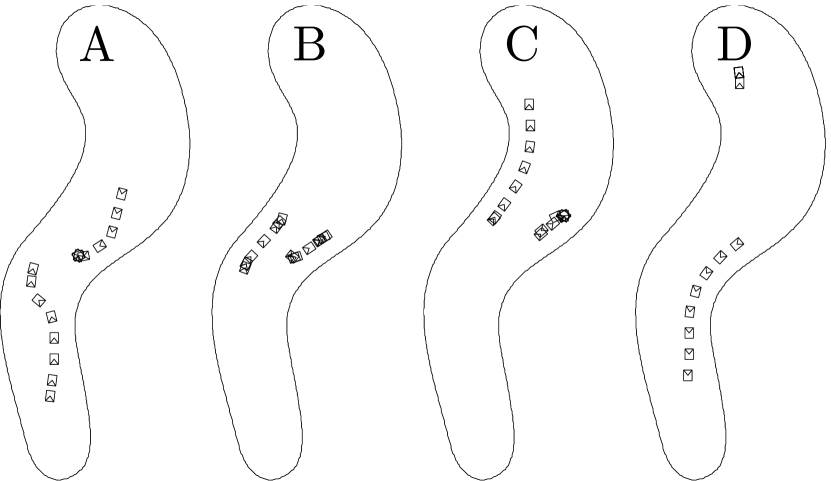
Figure 6.3: Simulations with deadlock avoidance (head-on encounter).

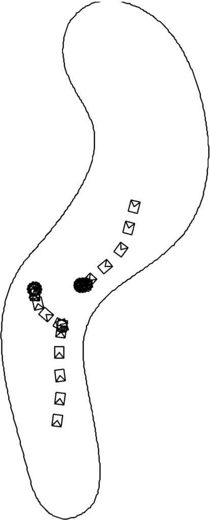
Figure 6.4: (a) Simulations without deadlock avoidance; (b) Simulations with deadlock avoidance (parallel encounter).

In Fig. 6.4(b), the approach is used a different topology of encounter, showings its versatility. The secondary vehicle loitered before the corridor before passing through.

Note that conditions that induce the recovery scheme were unable to be devised, and thus simulations of this part of the controller are not included here.

6.4 Experiments

Experiments were carried out with the identical experimental setup as Chapt. 5. The updated values of the parameters used in the experiments are listed in Table 6.2.

$R_{sen}$	$4.0m$
$d_{tar}$	$0.3m$
$v_{max}$	$0.5ms^{-1}$
$u_{\theta,max}$	$0.8rads^{-1}$
$u_{sp}$	$0.1ms^{-2}$

$\Delta\Lambda$	$0.50$
$c$	$1$
$\gamma_{1}$	$0.1$
$\gamma_{2}$	$0.001$

Table 6.2: Experimental parameters for deadlock-avoiding controller.

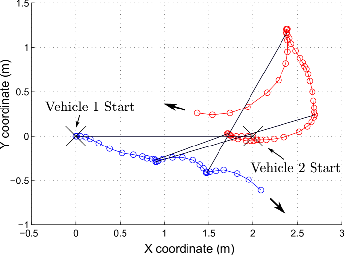
Figure 6.5: Trajectory for the experiment.

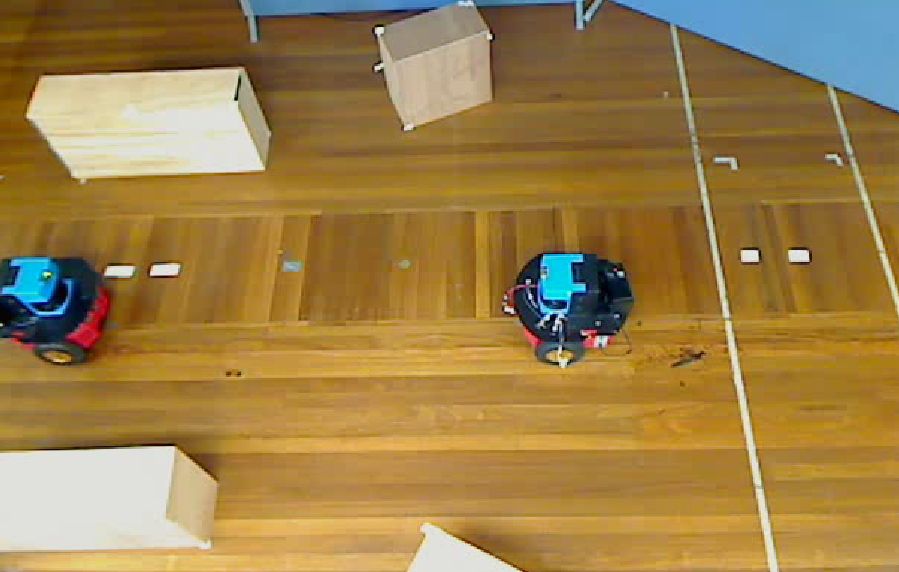
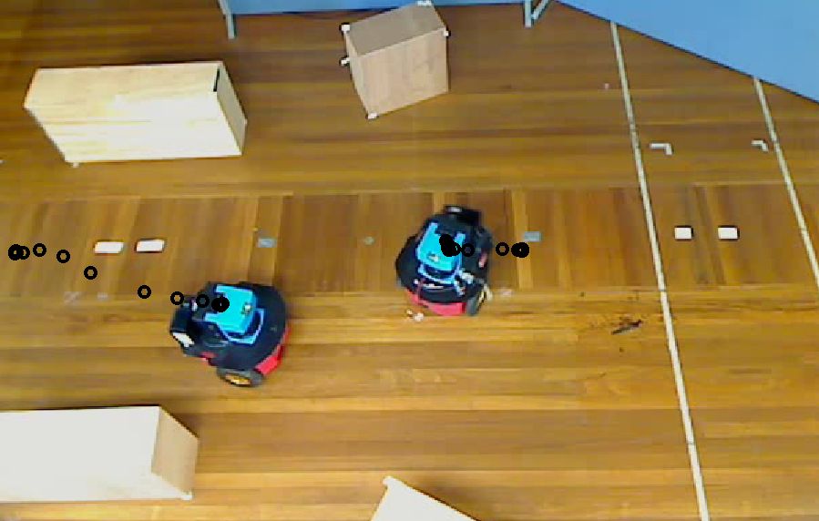
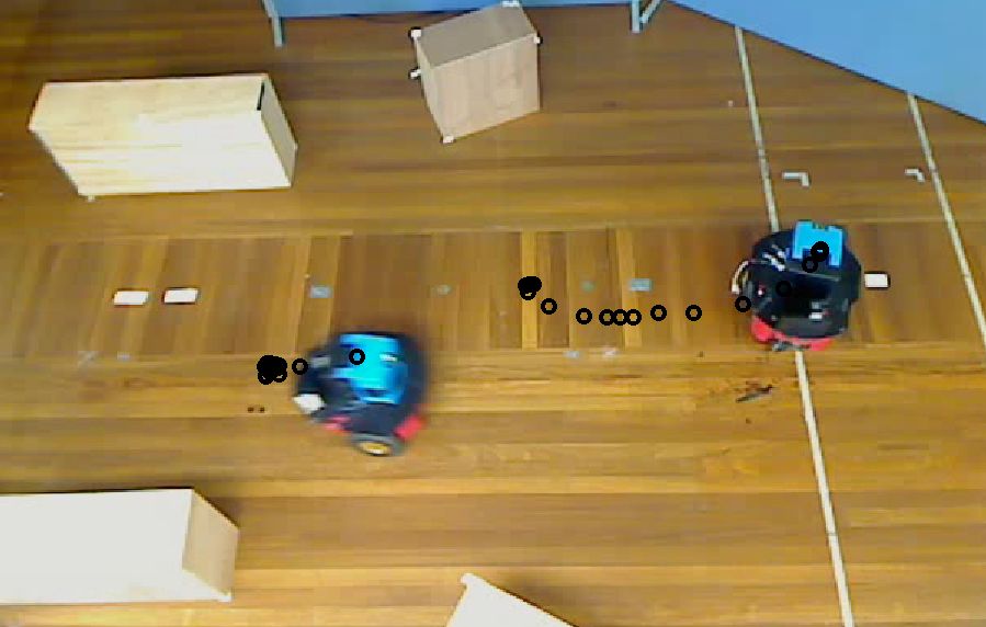
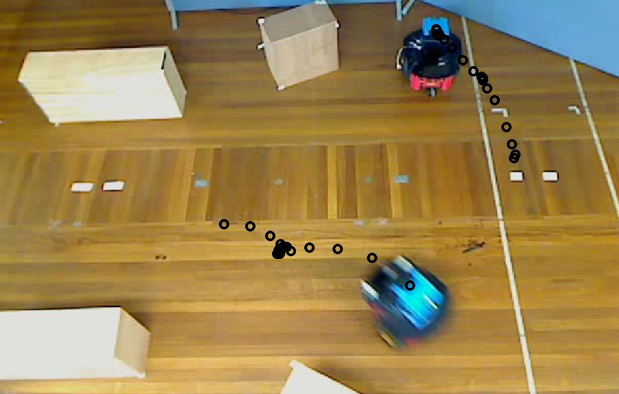
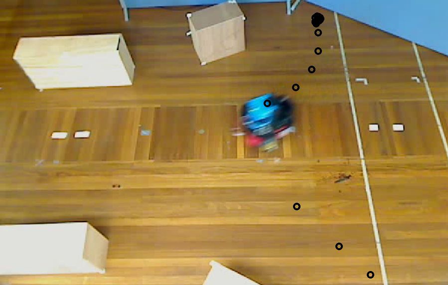
Figure 6.6: Sequence of images showing the experiment.

In the first scenario demonstrated by Figs. 6.6 and 6.5, the vehicles are both trying to move through a gap which is only wide enough for one vehicle. The secondary vehicle to the right allows the primary vehicle to the left to pass through before moving through itself.

6.5 Summary

In this chapter a method for reactively preventing deadlocks between two mobile vehicles is proposed. A hierarchy between the vehicles is enforced and the secondary vehicle always attempts to ensure the primary vehicle has a convergent trajectory to follow. While simulations show this approach is effective, it does not precipitate provable deadlock avoidance in all cases. As such, a less efficient recovery scheme which provably works in all conditions is provided. Future work will include more assumptions about obstacle and sensing requirements, which would be required to prove the main navigation system alone causes the vehicles to converge to their respective targets.

Chapter 7 Convergent Reactive Navigation using Minimal Information

In this chapter, information about the obstacle is limited to just the rate of change in the distance to the nearest point on the obstacle. This leads to a completely new control approach compared to the navigation laws proposed in Chapts. 3 to 6, where more information was assumed about the surrounding environment. Instead of path planning, a sliding mode control law is proposed which directly controls the control inputs of the vehicle. This means the navigation law has very low computational complexity, making it suitable for vehicles which have low computational capability – these are well exemplified by micro and miniature aerial vehicles.

Another advantage of the method proposed in this chapter is that global convergence to a target can be proven, where information about the target is limited to its bearing from the vehicles. Many reactive navigation methods such as artificial potential fields are not able to show this property. It can be achieved without randomization by using the Bug family of algorithms. Also, the Pledge [2] and Angulus [203] algorithms are in a similar vein.

These algorithms typically drive the robot directly towards the target when possible; otherwise, the obstacle boundary is followed in a close range. However, while very simple, they are not classed as reactive since a limited amount of information must be stored between control updates [203, 58]. In addition, a common problem with these strategies is that they typically take as granted the capability of carrying out specific maneuvers such as wall following, are disregard the kinematic constraints of the vehicle. Extending these methods to include such considerations basically lies in an uncharted territory.

Inspired by behaviors of animals, which are believed to use simple, local motion control rules that result in remarkable and complex intelligent behaviors [329, 47, 89], a navigation strategy is proposed that is aimed at reaching a steady target in a steady arbitrarily shaped maze-like environment and is composed of the following reflex-like rules:

1. At considerable distances from the obstacle,

   1. turn towards the target as fast as possible;

   2. move towards the target when headed for it;

2. In close proximity of the obstacle,

   1. Follow (a,b) when moving away from the obstacle;

   2. Otherwise, quickly avert the collision threat by making a sharp turn.

Studies of target pursuit in animals, ranging from dragonflies to humans, have suggested that they often use pure pursuit method s.1) to catch both steady and moving targets. The obstacle avoidance rule s.2) is also inspired by biological examples such as the near-wall behavior of a cockroach [47].

To address the issues of nonholonomic constraints, control saturation, and under-actuation, a vehicle of the Dubins car type is considered. It travels forward with a constant speed along planar paths of bounded curvatures and is controlled by the upper limited angular velocity. To implement s.1), s.2), only perceptual capabilities are needed that are enough to judge whether the distance to the obstacle is small or not, to estimate the sign of its time derivative, and to determine the polar angle of the target line-of-sight in the vehicle reference frame.

The convergence and performance of the proposed navigation and guidance law are confirmed by computer simulations and real world tests with a Pioneer P3-DX robot, equipped with a SICK LMS-200 LiDAR sensor.

All proofs of mathematical statements are omitted here; they are available in the original manuscript [223, 222].

The body of this chapter is organized as follows. In Sec. 7.1 the problem is formally defined, and in Sec. 7.2 the main assumptions are described. The main results are outlined in Sec. 7.3. Simulations and experiments are presented in Secs. 7.4 and 7.5. Finally, brief conclusions are given in Sec. 7.6.

7.1 Problem Statement

A planar vehicle is considered that travels forward with a constant speed $v$, and is controlled by the angular velocity $u$ limited by a given constant $\overline{u}$. There also is a steady point target $\boldsymbol{\mathscr{T}}$ and a single steady obstacle $D\not\ni\boldsymbol{\mathscr{T}}$, which is an arbitrarily shaped compact domain. Its boundary $\partial D$ is Jordan piece-wise analytical curve without inner corners (see Fig. 7.1(a)). Modulo smoothened approximation of such corners, this requirement is typically met by all obstacles considered in robotics. The objective is to drive the vehicle to the target with respecting a given safety margin $d(t)\geq d_{\text{safe}}>0\;\forall t$. The minimum distance to the obstacle is given as:

$$d(t):=\text{\bf dist}_{D}[\boldsymbol{r}(t)],\qquad\text{\bf dist}{\boldsymbol{r}}:=\min_{\boldsymbol{r}_{\ast}\in D}\|\boldsymbol{r}_{\ast}-\boldsymbol{r}\|,$$

Here $\boldsymbol{r}(t)$ is the robot location given by its abscissa $x(t)$ and ordinate $y(t)$ in the world frame. The orientation of the vehicle is described by the angle $\theta$ introduced in Fig. 7.1(b). The kinematics of the considered vehicles are classically described by the following equations:

$$\begin{array}[]{l}\dot{x}=v\cos\theta,\\ \dot{y}=v\sin\theta,\end{array},\quad\dot{\theta}=u\in[-\overline{u},\overline{u}],\quad\begin{array}[]{l}\boldsymbol{r}(0)=\boldsymbol{r}_{0}\not\in D\\ \theta(0)=\theta_{0}\end{array}.$$ (7.1)

Thus the minimal turning radius of the vehicle is equal to:

$$R=v/\overline{u}.$$ (7.2)

The vehicle has access to $d(t)$ and the signum $\text{\bf sgn}\,\dot{d}(t)$ if $d(t)\leq d_{\text{range}}$, where $d_{\text{range}}>d_{\text{safe}}$ is a given sensor range, and to the relative target bearing $\beta$ (see Fig. 7.1(b)). Mathematically, the examined strategy is described by the following equations:

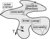
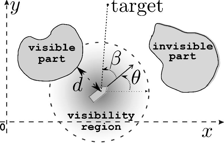
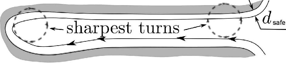
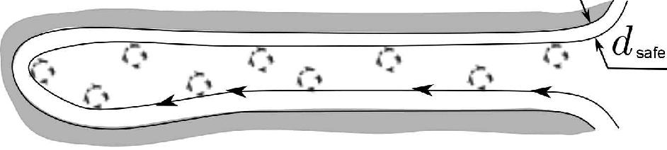
Figure 7.1: (a) Obstacle; (b) Planar vehicle; (c) Unavoidable collision; (d) Maneuverable enough vehicle.

$$u=\overline{u}\times\begin{cases}\text{\bf sgn}\beta\hfill\mid&\!\!\!\text{if}\;d>d_{\updownarrow}\;(\text{mode}\,\mathfrak{A})\\ \left\{\begin{array}[]{l l}\text{\bf sgn}\beta&\text{if}\;\dot{d}>0\\ -\sigma&\text{if}\;\dot{d}\leq 0\end{array}\right|&\!\!\!\text{if}\;d\leq d_{\updownarrow}\;(\text{mode}\,\mathfrak{B})\end{cases}.$$ (7.3)

Here $\sigma$ and $d_{\updownarrow}\in(0,d_{\text{range}})$ are controller parameters, and $\sigma$ can assume the values “+1” or “-1”. The former gives the turn direction in (d) and the latter regulates mode switching: $\mathfrak{A}\mapsto\mathfrak{B}$ when $d$ reduces to $d_{\updownarrow}$; $\mathfrak{B}\mapsto\mathfrak{A}$ when $d$ increases to $d_{\updownarrow}$. When mode $\mathfrak{B}$ is activated, $\dot{d}\leq 0$; if $\dot{d}=0$, the ‘turn’ submode $u:=-\sigma\overline{u}$ is set up.

In the basic version of the algorithm, $\sigma=\pm 1$ is fixed. As will be shown, the algorithms with $\sigma=+1$ and $\sigma=-1$ have basically identical properties except for the direction of bypassing the obstacle, which is counter clockwise and clockwise, respectively. To find a target hidden deep inside the maze, a randomized version can be used: whenever $\mathfrak{A}\mapsto\mathfrak{B}$, a new value of $\sigma$ is randomly generated from a fixed Bernoulli distribution over $+1,-1$.

7.2 Main Assumptions

It is assumed that the vehicle is maneuverable enough to avoid trapping in narrows of the maze (see Fig. 7.1(c,d)). Specifically, when following $\partial D$ with $d(t)=d_{\text{safe}}$, the full turn can always be made without violation of the safety margin. Furthermore, it is assumed this can be done without crossing a center of curvature of a concavity of $\partial D$, the normal radius of the osculating circle at a distance $\leq R$ from this center, and a location whose distance $d$ from $D$ is furnished by multiple points in $D$. This is required since at the respective points, the distance $d$ is uncontrollable – even if $\dot{d}(0)=0$, no control can prevent convergence to $D$: $\dot{d}(t)<0\;\forall t>0,t\approx 0$. For safety reasons, it is also assumed that $d_{safe}$ exceeds the unavoidable forward advancement $R$ during the sharpest turn.

Absence of inner corners implies that for any point from $\{\boldsymbol{r}\not\in D:\text{\bf dist}_{D}[\boldsymbol{r}]<d_{\star}\}$ with sufficiently small $d_{\star}>0$, the distance $\text{\bf dist}_{D}[\boldsymbol{r}]$ is attained at only one point $\boldsymbol{r}_{\star}\in\partial D$ and the curvature center does not lie on the straight line segment $[\boldsymbol{r}_{\star},\boldsymbol{r}]$ directed from $\boldsymbol{r}_{\star}$ to $\boldsymbol{r}$ [166]. The regular margin $d_{\star}(D)>0$ of $D$ is the supremum of such $d_{\star}$’s. Thus it follows:

$$d_{\star}(D)\leq R_{D}:=\inf_{\boldsymbol{r}\in\partial D:\varkappa(\boldsymbol{r})<0}R_{\varkappa}(\boldsymbol{r})$$ (7.4)

Here the variable $d_{\star}(D)=\infty$ if $D$ is convex. The variable $\varkappa(\boldsymbol{r}_{\ast})$ is the signed curvature ($\varkappa(\boldsymbol{r}_{\ast})<0$ on concavities), $R_{\varkappa}(\boldsymbol{r}_{\ast}):=|\varkappa(\boldsymbol{r}_{\ast})|^{-1}$, and $\inf$ over the empty set is set to be $+\infty$. Since the distance $d$ to $D$ may be increased by $2R$ during the full turn, the above assumptions can be summarized by the following equation:

$$d_{\star}(D)>d_{safe}+2R,\quad R_{D}>d_{safe}+3R,\quad d_{safe}>R.$$ (7.5)

It is also assumed that the sensor range is large enough to avoid violation of the safety margin after detection of $D$:

$$d_{\text{range}}>2R+d_{safe}.$$ (7.6)

This takes into account that even the sharpest turn may decrease $d$ by $2R$. As $d_{safe}\to R$, Eq.(7.5) and Eq.(7.6) shape into $\frac{v}{\overline{u}}=R<\min\left\{d_{\star}(D)/3;R_{D}/4;d_{\text{range}}/3\right\}$ and mean that the robot speed $v$ should not be large to cope with the maze. The following choice of $d_{\updownarrow}$ is feasible thanks to Eq.(7.5), Eq.(7.6):

$$d_{safe}+2R<d_{\updownarrow}<d_{\star}(D),d_{\text{range}},R_{D}-R,$$ (7.7)

7.3 Summary of Main Results

The $d$-neighborhood $\mathcal{N}(d)$ of $D$ is defined by $\mathcal{N}(d):=\{\boldsymbol{r}:\text{\bf dist}_{D}[\boldsymbol{r}]\leq d\}$. Let $\mathscr{D}\subset\mathbb{R}^{2}$ be a domain, $\boldsymbol{r}_{\lozenge},\boldsymbol{r}_{\ast}\in\partial\mathscr{D}$ lie on a common ray emitted from $\boldsymbol{\mathscr{T}}\not\in\mathscr{D}$, and $(\boldsymbol{r}_{\lozenge},\boldsymbol{r}_{\ast})\cap\mathscr{D}=\emptyset$. The points $\boldsymbol{r}_{\lozenge},\boldsymbol{r}_{\ast}$ divide $\partial\mathscr{D}$ into two arcs. Being concatenated with $[\boldsymbol{r}_{\lozenge},\boldsymbol{r}_{\ast}]$, each of them gives rise to a Jordan loop encircling a bounded domain, one of which is the other united with $\mathscr{D}$. The smaller domain is called the cave of $\mathscr{D}$ with corners $\boldsymbol{r}_{\lozenge},\boldsymbol{r}_{\ast}$. The location $\boldsymbol{r}$ is said to be locked in $\mathscr{D}$ if it lies in some cave of $\mathscr{D}$ (see Fig. 7.2).

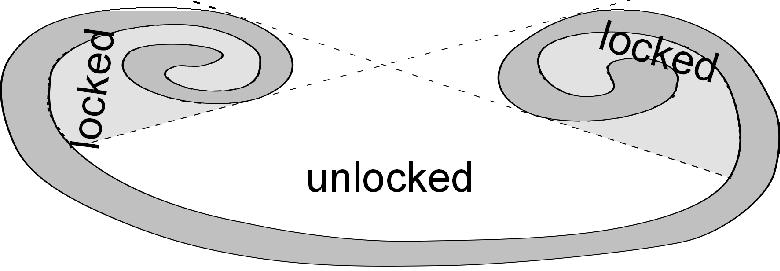
Figure 7.2: Locked locations

Theorem 7.3.1

Suppose that Eq.(7.5)–Eq.(7.7) hold, both the vehicle initial location $\boldsymbol{r}_{0}$ and the target $\boldsymbol{\mathscr{T}}$ are unlocked in $\mathcal{N}(d_{\updownarrow})$ and

$$\text{\bf dist}{\boldsymbol{r}_{0}}>d_{\updownarrow}+2R,\|\boldsymbol{r}_{0}-\boldsymbol{\mathscr{T}}\|>2R,\text{\bf dist}{\boldsymbol{\mathscr{T}}}>d_{\updownarrow}.$$ (7.8)

Then the basic control law brings the vehicle to the target in finite time without violation of the safety margin.

Dealing with a given obstacle may comprise several AM’s (i.e., motions in mode $\mathfrak{B}$); see Fig. 7.3(a). By ii) and iii), at most one both AM and SMEC is performed if $D$ is convex.

Fig. 7.3(b) offers an example where the basic control law fails to find a locked target. Fig. 7.3(c) shows that repeatedly interchanging left and right turns is not enough either. It can be shown that periodic repetition of any finite deterministic sequence of left and right turns is not enough to find the target in an arbitrary maze. Randomization overcomes the insufficiency of deterministic algorithms and aids to cope with uncertainty about the global geometry of complex scenes.

Figure 7.3: (a) Obstacle avoidance with two AM’s; (b,c) Insufficiency of (b) only-right-turns and (c) cycle-left-and-right-turns options.

7.4 Simulations

In simulations, the control was updated every $0.02$ seconds, $d_{\updownarrow}=8m$, $\overline{u}=2.5rad/s$, $v=3m/s$. Figs. 7.4(a,b) present typical results for the randomized controller, where the realizations $\sigma=+,-,-,-$ and $\sigma=-,+,+,+,-$ of the array of random turns were observed in (a) and (b), respectively.

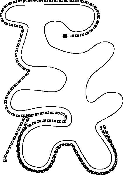
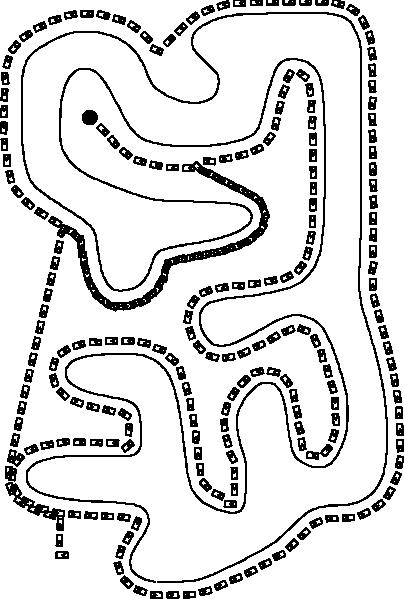
Figure 7.4: (a,b) Traversal to the target inside highly concave obstacles; (c) Performance under random noises.

To address performance under noises and un-modeled dynamics, the sensor readings and system equations were corrupted by independent Gaussian white noises with the standard deviation $0.1m$ for $d$, $0.1rad$ for $\beta$, $0.5rad/s$ for $\dot{\theta}$. To access $\dot{d}$, the difference quotient of the noisy data $d$ was computed with the time-step $0.1s$. The upper bound $\overline{u}$ on the turning rate $u$ was decreased to $0.7rad/s$, the threshold $d_{\updownarrow}$ was increased to $16m$, and extra dynamics were added via upper limiting $\dot{u}$ by $0.7rad/s^{2}$. Fig. 7.4(c) shows that the basic control law satisfactory guides the vehicle to the target for various realizations of the noises and disturbances.

7.5 Experiments

The use of switching regulation often gives rise to concerns about its practical implementation and implications of the noises and un-modeled dynamics in practical setting, including possible chattering at worst. To address these issues, experiments were carried out with an Activ-Media Pioneer 3-DX mobile robot using its on-board PC and the Advanced Robot Interface for Applications (ARIA 2.7.0), which is a C++ library providing an interface to the robot s angular and translational velocity set-points.

The position relative to the target was obtained through odometry, and $d_{\updownarrow}$ was taken to be 0.6 m and 0.9 m. The distance to the obstacles was accessed using both LIDAR and sonar sensors. A typical experimental result is presented on Fig. 7.5. In this experiment, like in the others, the robot reaches the target via safe navigation among the obstacles, with no visible mechanical chattering of any parts being observed.

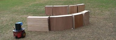
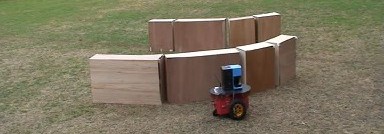
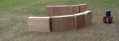
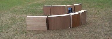
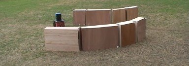
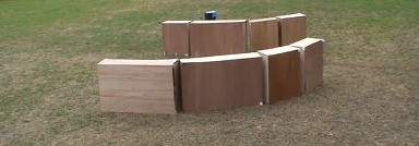
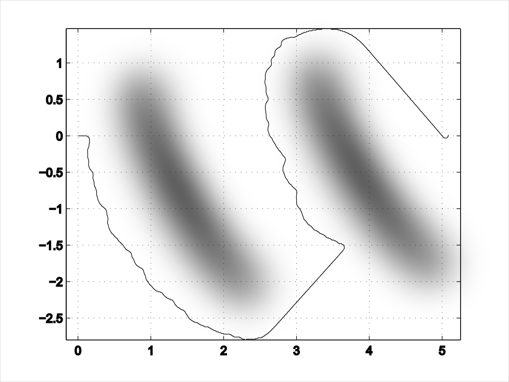
Figure 7.5: (a,b,c) Sequence of images obtained from real world experiments; (d) The trajectory of the robot, obtained through odometry.

7.6 Summary

The problem of safe navigation of a Dubins-car like robot to a target through a maze-like environment has been considered and a new bio-inspired control law has been proposed. The algorithm alternates between the pure pursuit navigation to the target and the sharpest turns away from the obstacle, with the latter being activated only at a short distance from obstacle and only if this distance decreases. Via computer simulations and experiments with real robots, it has been shown that this law constitutes an effective target-seeking strategy that can be realized even in complex maze-like environments.

Chapter 8 Convergent Reactive Navigation using Tangent Tracking

In previous chapters it was assumed that a finite sensor range was available to the vehicle. In this chapter it is assumed that instead of range information, the vehicle has knowledge of the relative heading of visible obstacle edges surrounding the vehicle. This is more similar to what would be obtained from a vision sensor.

The advantage of using a tangent sensor is that under certain conditions, the vehicle is able to follow the minimum length path. In this chapter, firstly the problem of global shortest path planning to a steady target in a known environment is considered. It is assumed that the environment contains a number of potentially non-convex obstacles, which have constraints imposed on their maximum curvature.

Secondly, a randomized navigation algorithm is propoposed, for which it can be shown that the robot will reach the target with probability $1$, while avoiding collision with the obstacles. The robot studied in this chapter is a unicycle like vehicle, described by the standard nonholonomic model with a hard constraint on the angular velocity.

Unlike many other papers on this area of robotics which present heuristic based navigation strategies, mathematically rigorous analysis is available for the navigation algorithm proposed in this chapter. Moreover, it should be pointed out that many other papers on this topic (see e.g. [302, 148, 147, 199]) do not assume non holonomic constraints on robot’s motion, which is a severe limitation in practice. The performance of this real-time navigation strategy is confirmed with extensive computer simulations and outdoor experiments with a Pioneer P3-DX mobile wheeled robot.

All proofs of mathematical statements are omitted here; they are available in the original manuscript [289].

The body of this chapter is organized as follows. In Sec. 8.1 the problem is formally defined, and in Sec. 8.2 the optimal off-line paths are described. A on-line navigation method is presented in Sec. 8.3. Simulations and experiments are presented in Secs. 8.4 and 8.5. Finally, brief conclusions are given in Sec. 8.6.

8.1 Problem Statement

A Dubins-type vehicle travelling at constant speed in the plane is considered, which has its maximum angular velocity limited by a given constant. The model of the vehicle is given as follows:

$$\begin{array}[]{l}\dot{x}=v\cos\theta\\ \dot{y}=v\sin\theta\\ \dot{\theta}=u\in[-u_{M},u_{M}]\end{array},\qquad\begin{array}[]{l}x(0)=x_{0}\\ y(0)=y_{0}\\ \theta(0)=\theta_{0}.\end{array}$$ (8.1)

Here $(x,y)$ is the vector of the vehicle’s Cartesian coordinates, $\theta$ gives its orientation, $v$ and $u$ are the speed and angular velocity, respectively. The maximal angular velocity $u_{M}$ is given. The robot satisfies the standard non-holonomic constraint:

$$|u(t)|\leq u_{M}$$ (8.2)

Also, the minimum turning radius of the robot is given by:

$$R_{min}=\frac{v}{u_{M}}.$$ (8.3)

Any path $(x(t),y(t))$ of the robot (8.1) is a plane curve satisfying the following constraint on its so-called average curvature (see [79]). Let $P(s)$ be this path parametrized by arc length; it is assumed the following contraint applies:

$$\|P^{\prime}(s_{1})-P^{\prime}(s_{2})\|\leq\frac{1}{R_{min}}|s_{1}-s_{2}|.$$ (8.4)

Notice that the constraint (8.4) on average curvature is used because the standard definition of curvature from differential geometry is not suitable (see e.g. [321]), since the curvature may not exist at some points of the robot’s trajectory.

There is a steady point-wise target ${T}$ and several disjoint obstacles $D_{1},\ldots,D_{k}$ in the plane. Let the safety margin $d_{0}>0$ be given. The objective is to drive the vehicle to the target through the obstacle-free part of the plane while keeping the safety margin.

Let $D$ be a closed set, $p$ be a point in the plain. Introduce the distance $\rho(D,p)$ given by:

$$\rho(D,p):=\min_{q\in D}\|p-q\|.$$

is set to zero if $p\in D$.

The following definition defines the neighborhood set of a point:

Definition 8.1.1

For $d_{0}>0$, the $d_{0}-$neighborhood of the domain $D\subset{\bf R}^{2}$ is the set formed by all points at the distance $\leq d_{0}$ from $D$, i.e., ${\cal N}[D,d_{0}]$ $:=$ $\{p\in{\bf R}^{2}:\rho(D,p)\leq$ $d_{0}\}$

The correct behavior of the system is defined as follows:

Definition 8.1.2

A path $p(t)=(x(t),y(t))$ of the robot (8.1) is said to be target reaching with obstacle avoidance if there exists a time $t_{f}>0$ such that $p(t_{f})={T}$ and $p(t)$ does not belong to ${\cal N}[D_{i},d_{0}]$ for all $i,t\in[0,t_{f}]$.

There are several assumptions which can now be made about the obstacle set:

Assumption 8.1.1

For all $i$ the set ${\cal N}[D_{i},d_{0}]$ is a closed, bounded, connected and linearly connected set. The sets ${\cal N}[D_{i},d_{0}]$ and ${\cal N}[D_{j},d_{0}]$ do not overlap for any $i\neq j$. For all $i$ the boundary $\partial D_{i}$ of the obstacle $D_{i}$ is a closed, non-self-intersecting analytic curve. For all $i$ the boundary $\partial D_{i}(d_{0})$ of the set ${\cal N}[D_{i},d_{0}]$ is a closed, non-self-intersecting analytic curve with curvature $k_{i}(p)$ at any point $p$ satisfying $|k_{i}(p)|\leq\frac{1}{R_{min}}$.

It is obvious that if Assumption 8.1.1 does not hold, target reaching with obstacle avoidance may be impossible (see e.g. Fig. 8.1).

Figure 8.1: Conditions for reaching the target.

It is also assumes that the initial position $p(0)=(x(0),y(0))$ of the robot is far enough from the obstacles and the target:

Assumption 8.1.2

The following inequalities hold: $\rho({\cal T},p(0))$ $\geq$ $8R_{min}$ and $\rho({\cal N}[D_{i},$ $d_{0}],p(0))$ $\geq$ $8R_{min}$ for all $i$. The robot initial heading $\theta(0)$ is not tangent to any boundary $\partial D_{i}(d_{0})$.

There are two circles with the radius $R_{min}$ that cross the initial robot position $p(0)$ and tangent to the robot initial heading $\theta(0)$. These are labeled initial circles.

8.2 Off-Line Shortest Path Planning

In this section, the shortest or minimum length target reaching paths with obstacle avoidance is described.

Definition 8.2.1

A straight line $L$ is said to be a tangent line if one of the following conditions holds:

1. The line $L$ is simultaneously tangent to two boundaries $\partial D_{i}(d_{0})$ and $\partial D_{j}(d_{0})$ where $i\neq j$.

2. The line $L$ is tangent to a boundary $\partial D_{i}(d_{0})$ on two different points.

3. The line $L$ is simultaneously tangent to a boundary $\partial D_{i}(d_{0})$ and an initial circle.

4. The line $L$ is tangent to a boundary $\partial D_{i}(d_{0})$ and crosses the target ${T}$.

5. The line $L$ is tangent to an initial circle and crosses the target ${T}$.

Points of boundaries $\partial D_{i}(d_{0})$ and initial circles belonging to tangent lines are called tangent points. Consider only finite segments of tangent lines such that their interiors do not overlap with any boundary $\partial D_{i}(d_{0})$. The segments of tangent lines of types $1)$ and $2)$ are called $(OO)-$segments, the segments of tangent lines of type $3)$ are called $(CO)-$segments, the segments of tangent lines of type $4)$ are called $(OT)-$segments, and the segments of tangent lines of type $5)$ are called $(CT)-$segments. Furthermore, only segments that do not intersect the interiors of the initial circles are considered.

Definition 8.2.2

A segment of a boundary $\partial D_{i}(d_{0})$ between two tangent points is called $(B)-$segment if curvature is non-negative at any point of this segment (see Fig. 8.2). A segment of an initial circle between the initial robot position $p(0)$ and a tangent point is called $(C)-$segment (see Fig. 8.3).

Figure 8.2: A $(B)-$segment.

Figure 8.3: A $(C)-$segment.

Now the main result of this section may be presented:

Theorem 8.2.1

Suppose that Assumptions 8.1.1 – 8.1.2 hold. Then there exists a shortest (minimum length) target reaching path with obstacle avoidance. Furthermore, a shortest target reaching path consists of $n\geq 2$ segments $S_{1},S_{2},\ldots,S_{n}$ such that if $n=2$ then $S_{1}$ is a $(C)-$segment and $S_{2}$ is a $(CT)-$segment. If $n\geq 3$ then $S_{1}$ is a $(C)-$segment, $S_{2}$ is a $(CO)-$segment and $S_{n}$ is a $(OT)-$segment. If $n>3$ and $3\leq k\leq n-1$ then any $S_{k}$ is either $(OO)-$segment or $(B)-$segment.

Figure 8.4: An example of the tangent graph, with a target point $T$.

8.3 On-Line Navigation

In this section, the case of sensor based on-line navigation is considered, where the robot does not know the location of the target and the obstacles a priori. The robot is equipped with a vision type sensor which is able to determine coordinates of the target and points of the boundaries $\partial D_{i}(d_{0})$ if the straight line segment connecting the robot current coordinates and the point of interest does not intersect any obstacle $D_{i}$ (see Fig. 8.5).

Figure 8.5: Vision sensor model of the robot.

Definition 8.3.1

When the robot moves along the boundary of an obstacle or an initial circle and reaches a tangent point, it can leave the boundary and move along the corresponding straight line edge of the tangent graph if its heading is equal to direction of this edge (see Fig. 8.6a). In this case, the robot is said to have reached an exit tangent point. (A case when the robot cannot leave the boundary at a tangent point is shown on Fig. 8.6b). Furthermore, if the straight line edge corresponding to this exit tangent point is an $(OT)$ or $(CT)$ segment, then this point is called an exit tangent point of $T-$type. Otherwise, if the straight line edge corresponding to this exit tangent point is an $(OO)$ or $(CO)$ segment, this point is called an exit tangent point of $O-$type.

Figure 8.6: Conditions for a tangent segment to be transversed.

Let $0<p<1$ be a given number. To solve this problem, the following probabilistic navigation algorithm is proposed:

A1: The robot starts to move along any of two initial circles.

A2: When the robot moving along an obstacle boundary or an initial circles reaches an exit tangent point of $T-$type, it starts to move along the corresponding $(OT)$ or $(CT)$ segment.

A3: When the robot moves along an obstacle boundary or an initial circle and reaches an exit tangent point of $O-$type, with probability $p$ it starts to move along the corresponding $(CO)$ or $(OO)$ segment, and with probability $(1-p)$ it continues to move along the boundary.

A4: When the robot moves along a $(CO)$ or $(OO)$ segment and reaches a tangent point on an obstacle boundary, it starts to move along the obstacle boundary.

Now the main result of this section may be presented:

Theorem 8.3.1

Suppose that Assumptions 8.1.1 – 8.1.2 hold. Then for any $0<p<1$, the algorithm A1–A4 with probability $1$ defines a target reaching path with obstacle avoidance.

8.4 Simulations

In this section, computer simulations of the reactive navigation algorithm A1–A4 are presented. This navigation strategy was realized as a sliding mode control law, by switching between a boundary following approach proposed in [230], and the pure pursuit navigation approach (see e.g. [291]). The navigation law can be expressed as follows:

$$u(t)=\left\{\begin{array}[h]{cc}\pm u_{M}&R1\\ \Gamma sgn\left[\varphi_{tan}(t)\right]u_{M}&R2\\ \Gamma sgn\left[\dot{d}_{min}(t)+X(d_{min}(t)-d_{0})\right]u_{M}&R3\\ \end{array}\right.\\$$ (8.5)

$$R1\rightarrow R2 : CO\text{ or }CT\text{ detected}$$

$$R2\rightarrow R3 : d_{min}(t)<d_{trig},\dot{d}_{min}(t)<0$$

$$R3\rightarrow R2 : \left\{\begin{array}[]{l}OT\text{ detected}\\ OO\text{ detected, probability }p\end{array}\right.$$ (8.8)

This navigation law is a rule for switching between three separate modes $R1-R3$. Initially mode $R1$ is active, and transitions to other modes are determined by equation (8.4). Mode $R1$ describes motion along the initial circle with maximal actuation. Mode $R2$ describes pursuit navigation, where $\varphi_{tan}(t)$ is defined as the angle between the vehicle’s heading and a line segment connecting the vehicle and currently tracked tangent edge (see equation (8.11)). Mode $R3$ describes boundary following behaviour, where the control calculation is based on the minimum distance to the nearest obstacle, defined as $d_{min}(t)$. This control law is subject to some restrictions which are inherited from [230], however these are satisfied due to the assumptions in Sec. 8.1. The variable $\Gamma$ is defined as $+1$ if the obstacle targeted is on the left of the tangent being tracked, $-1$ if it is on the right. A constant $d_{trig}>d_{0}$ is also introduced which determines when the control system transitions to boundary following mode [230]. The saturation function $X$ is defined as follows:

$$X(r)=\left\{\begin{array}[h]{cc}lr&|r|<k\\ lk\ sgn(r)&otherwise\\ \end{array}\right.$$ (8.10)

Here $l$ and $k$ are tunable constants. Because of any potential chattering in the output, once it is decided to not pursue a tangent, there is a short pause until tangent following can potentially be engaged again.

Remark 8.4.1

Notice that it follows from (8.1) that the robot’s trajectory is differentiable. This and Assumption 8.1.1 imply that the function $d_{min}(t)$ is continuous, however, in the case on a non-convex obstacle, the function $d_{min}(t)$ may be non-differentiable for some $t$. It does not really matter in practice, in these computer simulations and experiments with a real robot, the first order difference approximation of $\dot{d}_{min}(t)$ in the equation (8.5) is used.

In these simulations and experiments, the robot is assumed to posess a LiDAR-type device, which informs the vehicle of the distance from the vehicle to obstacle in a finite number of directions around the obstacle. The length of these detection rays are defined by $\eta_{i}$, where $\eta_{0}$ refers to a detection ray directly in front of the vehicle. The angular spacing between successive rays is defined $\Delta\theta$. In this case a tangent in front of the vehicle is detected by monitoring $|\Delta\eta_{0}|$ for any changes beyond some threshold $d_{thresh}$. The transversal direction can be determined by comparing the immediately adjacent obstacle detections; $\Gamma:=\text{\bf sgn}(\eta_{1}-\eta_{-1})$.

To calculate the error parameter $\varphi_{tan}$, a point $T_{int}$ is defined as an intermediate target. This is calculated by iteration of the following steps:

1) Initially when $R2$ is engaged, the $T_{int}$ is set to be a constant offset from the detected tangent point:

$$T_{int}=\left[\begin{array}[]{c}x(t)+cos(\theta(t)+i\Delta\theta+\Gamma\tan^{-1}(d_{0}/d_{cen}(t)))\\ y(t)+sin(\theta(t)+i\Delta\theta+\Gamma\tan^{-1}(d_{tar}/d_{cen}(t)))\end{array}\right]$$ (8.11)

with $i:=0$.

2) $\varphi_{tan}$ is calculated by finding the angle between the vehicle heading and a line connecting the vehicle and $T_{int}$.

3) In subsequent time steps a successive tangent point is found; a search occurs for the appropriate $i$ so that $\eta_{i}-\eta_{i+\Gamma}>d_{thresh}$ (so the same transversal direction as the stored intermediate target is maintained), and also has the smallest Euclidean distance to $T_{int}$. The point is calculated using equation (8.11).

Remark 8.4.2

While this calculation calls for an estimate of position to be available to the robot, this estimate only needs to be accurate for a relatively short time between control updates. Thus in the studied case, robot odometry is sufficient since robot odometry gives an accurate estimate over short time intervals.

$u_{max}$	$1.3rads^{-1}$
$v$	$1.5ms^{-1}$
$d_{tar}$	$5m$

$d_{trig}$	$10m$
$l$	$0.33$
$k$	$15m$

$p$	$0.7$
$d_{thresh}$	$10m$

Table 8.1: Simulation parameters for tangent-following controller.

Figure 8.7: Simulation with a simple environment.

Figure 8.8: Simulation with a challenging environment.

Figure 8.9: Simulation with a more challenging environment.

The following simulation was carried out with the unicycle model (8.1) and the navigation law updated at 10 Hz. Parameters used for simulations may be found in Table 8.1. In Figs 8.7, 8.8 and 8.9, it can be seen that the robot converges to the target without any problems, as expected. Different sequences of random numbers would of course lead to different paths around the obstacles.

8.5 Experiments

In this section, an implementation of the reactive navigation algorithm A1–A4 is presented. Experiments were carried out with a Pioneer P3-DX mobile robot. A LiDAR device with an angular resolution of $1^{o}$ was used to detect tangents directly ahead of the robot as well as obstacles in the vicinity of the robot. In the scenario tested the vehicle was not provided with a target, rather it was allowed to patrol the area indefinitely. Odometry information available from the robot was used over a single time step to compensate for the movement of the previously calculated tangent point relative to the vehicle, as explained in the previous section (see Remark 5.1). Range readings over a maximum threshold $R_{max}$ were truncated, in order to prevent any object outside the test area from influencing the results. Parameters used for experiments are shown in Table 8.2.

Measures were also included to reduce control chattering, which can cause detrimental effects when using real robots [327]. The signum function of equation (8.5) was replaced by a saturation function - equation (8.10) with $l=k=1$), and the standard low level controller on the robot was modified to filter high frequency control inputs.

$v$	$0.25ms^{-1}$
$d_{tar}$	$1m$
$d_{trig}$	$1.5m$

$l$	$0.1$
$k$	$1.0m$
$p$	$0.7$

$R_{max}$	$6m$
$d_{thresh}$	$1m$

Table 8.2: Experimental parameters for tangent-following controller.

Figure 8.10: Sequence of images showing the experiment.

The vehicle successfully navigates around the obstacles without collision, as indicated in Fig. 8.10.

8.6 Summary

The shortest (minimal in length) path for a unicycle-like mobile robot in a known environment is described, which contains smooth (possibly non-convex) obstacles. Furthermore, a reactive randomized algorithm for robot navigation in unknown environments is proposed. The performance of this algorithm has been confirmed by computer simulations and outdoor experiments with a Pioneer P3-DX mobile wheeled robot.

Chapter 9 Nonlinear Sliding Mode Control of an Agricultural Tractor

This chapter considers the problem of automatic path tracking by autonomous farming vehicles subject to wheel slips, which are characteristic for agricultural applications. The control law used is similar to the one employed in Chapt. 3 to regulate the position of a unicycle-type vehicle. Simulations compare the performance of this mixed nonlinear-sliding mode control law with both a pure sliding mode control law and another control law proposed in the literature. Real world experiments confirm the applicability and performance of the proposed guidance approach.

9.1 Introduction

Automatic guidance of agricultural vehicles is a widely studied problem in robotics. Such automatic systems are aimed at replacement of human beings in tedious or hazardous operations, and improve productivity while reducing work hardness. Driver assistance devices and automatic steering systems have attracted considerable interest (see e.g. [153, 271]). The reported systems provide satisfactory performance if the motion is nearly pure rolling without slip – wheel slips usually causing visible performance degradation. Unfortunately, slipping effects commonly occur during agricultural tasks since the farming terrain is often non-smooth and undulating, and the vehicle is affected by disturbances from the towed implements interacting with the ground.

There is an extensive literature on path following control of wheeled vehicles in the no-slip circumstances, see e.g. [38, 45, 267]. Even in this case, the problem is rather challenging. Due to the nonholonomic nature, the system cannot be asymptotically stabilized by a smooth time-invariant feedback [43]. Slip effects can be incorporated into this analysis if exact knowledge of the slipping parameters is available [248]. Slipping has also been modeled as fast dynamics, with a singular perturbation approach being used to achieve robust tracking under sufficiently small sliding [67, 193]. Asymptotic tracking has been achieved for slightly curved reference paths using a time varying controller [192]. Adaptive control has been proposed in the form of adaptive back-stepping and adaptive re-scheming of the desired path [185, 92, 93, 187]. A differential flatness approach has been applied to a car-like robot controlled by both steering and front-wheel drive speed, however rear wheel drive vehicles are mostly employed in agricultural applications [5]. A MPC element has been proposed to account for actuator delay when added to a control law [187]. Kinematic control law in combination with dynamic observers estimating slip parameters have been used to achieve improved path tracking accuracy [190, 191, 90].

Due to the well-known benefits, such as stability under large disturbances and robustness against system uncertainties, the sliding mode approach attracts an increasing interest in the area of agricultural vehicles control. A discrete-time sliding mode control has been proposed for trajectory tracking in the presence of skidding effects [63]. The sliding mode approach has also been used to achieve global lateral stabilization via steering actuation only [127]. Here the drive speed was assumed constant and the slipping effects were represented by additive disturbances in the ideal kinematic model, both in the original and in the transformed chained forms. The ideal kinematic equations can also be modified to include slip-induced biases in the steering angle and drive speed [82]. Assuming full actuation, this chapter reports successful use of the combined sliding mode and back-stepping techniques to achieve both lateral and longitudinal stabilization. A similar problem has been treated along the lines of the singular perturbation approach, and the problem was solved using a second order sliding mode control [126, 67]. However, for some agricultural applications, the precise longitudinal stabilization is of minor importance, in which case the only-steering control is a reasonable option.

The characteristic feature of the above works is the lack of concern for the actual steering capabilities of the vehicle. The stability of path tracking is guaranteed only under the implicit and unjustified assumption that the outputs of the proposed sophisticated nonlinear controller always obey the mechanical steering angle limit. This is definitely plausible in favorable circumstances. Unfortunately, wheel slippage, large lateral disturbances and sharp contortions in the reference path may require the vehicle to operate near the steering angle limit, and this may lead to excessively large controller outputs and thus violation of the above assumption. This is a likely cause for systematic occasional degradation of the tracking accuracy observed for existing laws.

From the more general perspective, there is only limited literature available about stabilization and tracking of nonholonomic wheeled vehicles with input saturations. For nonholonomic systems in chained form, discontinuous controllers obeying a given bound and stabilizing an equilibrium have been obtained [205, 8]. A passivity-based approach has been applied to stabilize equilibria of special controllable drift-less systems using a time-varying smooth state feedback controller [196]. Semi-global practical stabilizing control schemes for wheeled robots with two steering wheels and one castor wheel have also been proposed [348]. However, all these works did not treat path tracking. This issue has been addressed using passivity-based, saturated, Lipschitz continuous, time-varying feedback laws for unicycles with forward and turning velocity bounds [143]. Trajectory tracking controllers for nonholonomic robots with fixed-wing UAV-like input constraints and experimental results on their performance are also available [274]. The characteristic feature of these works is the use of unnecessary and non-conservative bounds on controller outputs, which in general does not permit the controller to employ the full range of the vehicle’s steering capabilities and may cause performance degradation in challenging circumstances. Another restriction is that these works assume pure wheels rolling without slipping. Off-road path tracking with both wheel slip and explicit concern for steering saturation has been addressed, using a model predictive algorithm for the longitudinal speed adjustment. This enables the main steering controller to be decoupled and be borrowed from [186, 190, 191], which can adaptively cope with contortions of the reference path during cornering in the face of wheel slip and steering angle limit. However even in this work, the design of the steering controller still neglects this limit.

To fill this gap, in this chapter the problem of globally stable tracking of an arbitrarily curved path via bounded steering only is considered – the nominal drive speed is constant and the controller must ensure that the steering angle bound is always satisfied. Following [93, 188, 239, 91], the slipping effects are modeled via biases of the steering angle and vehicle velocity in the ideal kinematic equations, where they are treated as bounded uncertainties. To design a controller, a sliding mode approach is employed. Unlike the previous research, the requirements to the sliding surface that are imposed by the steering angle limit are explicitly disclosed. To fully use the steering capabilities of the vehicle, the optimal surface among those satisfying these requirements is found – this surface minimizes the maximal steady-state error. Furthermore, the proposed sliding mode control laws do not artificially impede the steering angle within the given limits. Two control laws are examined and compared. The first of them is a pure sliding-mode controller that formally requests only limit values of the steering angle. As was discovered via simulation tests and experiments, this controller may cause an oscillatory behavior in some cases. So it was used as a theoretical platform for design of the second law that combines a smooth nonlinear control with switching in the sliding-mode fashion between reduced limits determined only by the need to reject the slipping effects. The smooth control is in fact the equivalent control for the first law [339]. More precisely, since computation of the equivalent control requires unknown slip parameters, a reasonable approximation is used.

The applicability and performance of the proposed control law is validated via computer simulations and real world testing using an agricultural vehicle.

All proofs of mathematical statements are omitted here; they are available in the original manuscript [220].

The body of this chapter is organized as follows. Secs. 9.2 and 9.3 introduce the problem setup and the employed kinematic model. Sec. 9.4 offers the study of sliding surfaces; the proposed control laws are discussed in Secs. 9.5 and 9.6. Sec. 9.7 presents the simulation results, and experimental results are presented in Sec. 9.9. Finally, brief conclusions are given in Sec. 9.10.

9.2 Problem Statement

A planar wheeled mobile robot modeled as a bicycle with front steering is considered. It is controlled by the front wheels steering angle and travels with the constant rotating angular velocity of the rear wheels. The objective is to follow a given reference path as close as possible. To describe the robot motion, the relative vehicle-fixed normally oriented Cartesian coordinate system with the $x$-axis directed along the vehicle centerline from rear to front is introduced, along with the following variables (see Fig. 9.1):

• $\mathfrak{F}$ – the center of the front wheels axle;

• $\mathfrak{R}$ – the center of the rear wheels axle;

• $s$ – the curvilinear abscissa of the point on the reference path that is closest to $\mathfrak{R}$, the path is oriented so that $s$ ascends in the required motion direction;

• $r(s)\in\mathbb{R}^{2}$ – a regular parametric representation of the reference path in the world frame;

• $[T(s),N(s)]$ – the Frenet frame of the path at $r(s)$: $T(s)$ is the unit positively oriented tangential vector, $N(s)$ is the unit normal, the frame is normally oriented;

• $\varkappa(s)$ – the signed curvature of the reference path: $\varkappa=\left\langle T^{\prime};N\right\rangle$, where ^′ is differentiation with respect to $s$ and $\left\langle\cdot;\cdot\right\rangle$ is the standard inner product in the plane $\mathbb{R}^{2}$;

• $z$ – the $N$-coordinate of $\mathfrak{R}$ in the Frenet frame;

• $\vec{V}$ – the velocity of the point $\mathfrak{R}$ in the world frame;

• $\vec{V}_{\text{F}}$ – the velocity of the point $\mathfrak{F}$ in the world frame;

• $v$ – the speed of the point $\mathfrak{R}$, i.e., $v=\|\vec{V}\|$;

• $\varphi$ – the rear wheel slip angle, i.e., the angular polar coordinate of $\vec{V}$ in the relative coordinate system;

• $\theta$ – the angular polar coordinate of the tangential vector $T(s)$ in the relative coordinate system;

• $\delta$ – the steering angle of the front wheels;

• $\delta_{\max}$ – the maximal steering angle: $\delta\in[-\delta_{\max},\delta_{\max}]$;

• $\beta$ – the steering angle bias due to sliding;

• $L$ – the vehicle wheelbase;

• $v_{\text{rw}}$ – the driving speed: $v_{\text{rw}}=\rho\cdot\omega_{\text{r}}$, where $\rho$ is the radius of the rear wheel and $\omega_{\text{r}}$ is its angular velocity;

• $v_{\text{rw}}^{\text{s}}$ – the bias of the driving speed due to wheels slip, i.e., the projection of the velocity of the rear wheel point of contact with the ground on the vehicle centerline.

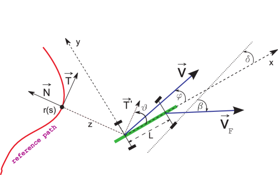
Figure 9.1: Basic variables and constants.

The objective is to design a controller such that

$$z\to 0\qquad\text{as}\quad t\to\infty.$$

To this end, the vehicle is equipped with sensors that ensure access to the positional $z$ and angular $\theta$ errors of the path following. There also is an access to the path curvature $\varkappa(s)$.

Direct measurement of the slip parameters $\varphi,\beta$, and $v_{\text{rw}}^{\text{s}}$ is hardly possible at a reasonable cost (see e.g., [319]). So they are treated as bounded system uncertainties:

$$|\varphi|\leq\overline{\varphi},\quad|\beta|\leq\overline{\beta},\quad\left|v_{\text{rw}}^{\text{s}}\right|\leq\overline{v}.$$ (9.1)

It is assumed that the wheels slip can reverse neither the translational nor, under the maximum steering angle, angular directions of the vehicle motion:

$$\overline{v}<v_{\text{rw}},\qquad\overline{\beta}<\delta_{\max}.$$ (9.2)

In agricultural applications, the biases $\varphi,\beta$ are usually small ($\approx$ several degrees) [91]. For technical reasons, it is assumed:

$$\overline{\varphi}<\pi/2,\qquad\overline{\beta}<\pi/2.$$ (9.3)

Through not required, indirect on-line estimates $\widehat{\varphi}$ and $\widehat{\beta}$ of $\varphi$ and $\beta$, may be available, with the errors:

$$\left|\varphi-\widehat{\varphi}\right|\leq\overline{\varphi}_{\text{est}},\qquad\left|\beta-\widehat{\beta}\right|\leq\overline{\beta}_{\text{est}}.$$ (9.4)

If estimation is not carried out, $\widehat{\varphi}:=\widehat{\beta}:=0$ and so $\overline{\varphi}_{\text{est}}=\overline{\varphi},\overline{\beta}_{\text{est}}=\overline{\beta}$. The estimates are supposed to be improvable via neither annihilation nor saturation at the bound from Eq.(9.1):

$$\overline{\varphi}_{\text{est}}\leq\overline{\varphi},\quad\overline{\beta}_{\text{est}}\leq\overline{\beta},\quad|\widehat{\varphi}|\leq\overline{\varphi},\quad|\widehat{\beta}|\leq\overline{\beta}.$$ (9.5)

It is also assumed that $\varphi,\widehat{\varphi},\beta,\widehat{\beta},v_{\text{rw}}^{\text{s}}$ continuously depend on time $t$.

9.3 Kinematic Model

Basic assumptions are given as follows:

Assumption 9.3.1

The reference path is $C^{1}$-smooth and $C^{2}$-piece-wise smooth regular curve. The curvature of the reference path is upper bounded:

$$\overline{\varkappa}:=\sup_{s}|\varkappa(s)|<\infty.$$ (9.6)

Assumption 9.3.2

The vehicle is capable of tracking the reference path: the path curvature radius at any point is no less than the minimal turning radius $R=\frac{L}{\tan\delta_{\max}}$ of the vehicle. Moreover, the associated strict inequality holds:

$$\overline{\varkappa}<\varkappa_{\text{v}}:=R^{-1}=L^{-1}\tan\delta_{\max}.$$ (9.7)

Vehicle maneuvers are examined at distances not exceeding the curvature radius of the reference path:

$$|z|\leq\overline{\varkappa}^{-1}\lambda$$ (9.8)

Here $0<\lambda<1$ is a given parameter. Hence the point on the path that is closest to $\mathfrak{R}$ is well defined and smoothly depends on the vehicle position. The kinematic equations given by the following lemma are borrowed from [239, 91, 188, 141]:

Lemma 9.3.1

The vehicle kinematic model is as follows:

$$\dot{s}=\frac{v\cos(\theta-\varphi)}{1-\varkappa(s)z},\;\dot{z}=-v\sin(\theta-\varphi),\;v=\frac{v_{\text{rw}}+v_{\text{rw}}^{\text{s}}}{\cos\varphi},$$ (9.9)

$$\dot{\theta}=\varkappa(s)\frac{v\cos(\theta-\varphi)}{1-\varkappa(s)z}-\frac{v}{L}\left[\tan(\delta+\beta)-\tan\varphi\right].$$ (9.10)

9.4 Desired Dynamics

This chapter is concerned with relations of the form:

$$\theta=\chi(z)+\widehat{\varphi}.$$ (9.11)

It is assumed that $\chi(\cdot)$ is an odd ascending continuous piece-wise smooth function such that $\frac{d\chi}{dz}(z\pm 0)>0$ whenever $-\mu<\chi(z)<\mu:=\chi(\lambda/\overline{\varkappa})$ (see Fig. 9.2). A simple sample employed here is the linear function with saturation: $\chi(z):=\gamma z$ if $|z|\leq\Delta$ and $\chi(z):=\mu\text{\bf sgn}(z)$ otherwise. Here $\mu:=\gamma\Delta$ and $\gamma>0,0<\Delta\leq\lambda/\overline{\varkappa}$ are design parameters.

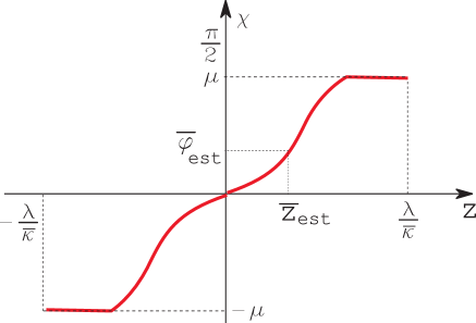
Figure 9.2: The desired relation $\theta=\chi(z)$.

9.4.1 Conditions for Robustly Stable Path Tracking

The first lemma characterizes the positional error caused by the errors in estimation of the wheels slip parameters.

Lemma 9.4.1

Let the motion starts in the domain Eq.(9.8),

$$\overline{\varphi}_{\text{est}}<\mu:=\chi\left(\lambda/\overline{\varkappa}\right)<\pi/2-\overline{\varphi}_{\text{est}},$$ (9.12)

and let $\overline{z}_{\text{est}}$ denote the unique root of the equation $\chi(\overline{z}_{\text{est}})=\overline{\varphi}_{\text{est}}$. Whenever Eq.(9.11) is maintained during the motion, the vehicle remains in the domain Eq.(9.8) and the positional error $|z|$ of the path following monotonically decays to $\overline{z}_{\text{est}}$. This decay either is asymptotical $|z(t)|\xrightarrow{t\to\infty}\overline{z}_{\text{est}},|z(t)|>\overline{z}_{\text{est}}\;\forall t$ or is completed for a finite time $\exists t_{\ast}:|z(t)|\leq\overline{z}_{\text{est}}\;\forall t\geq t_{\ast}$. In any case, the decay is at no less than the exponential rate:

$$|z(t)|\leq\overline{z}_{\text{est}}+ce^{-\gamma\left(v_{\text{rw}}-\overline{v}\right)t},\qquad\gamma:=\frac{d\chi}{dz}(\overline{z}_{\text{est}}+0).$$ (9.13)

9.4.2 Feasibility of the Desired Dynamics

Restrictions on the vehicle steering angle may make maintenance of relation Eq.(9.11) unrealistic. To disclose the conditions under which this is not the case, the following is introduced:

Definition 9.4.1

Relation Eq.(9.11) is said to be nominally maintainable in the domain Eq.(9.8) if whenever it is achieved $S:=\theta-\chi(z)-\widehat{\varphi}=0$ at a vehicle position from this domain, it can be maintained by a proper choice of the front wheels steering angle: $\exists\delta\in[-\delta_{\max},\delta_{\max}]:\dot{S}(\delta)=0$.

It is assumed here that the choice of $\delta$ is based on not only the measured data $z,\theta,\varkappa(s)$ and available estimates $\widehat{\varphi},\widehat{\beta}$ but also on access to the slip uncertainties $\varphi,\beta,v^{s}_{\text{rw}}$. It will be shown that conditions necessary for maintainability of Eq.(9.11) in these idealized circumstances are ‘almost sufficient’ for its maintainability in the realistic case where the above uncertainties are unknown.

Lemma 9.4.2

Relation Eq.(9.11) is nominally maintainable in the region Eq.(9.8) if

$$\varkappa_{\text{v,u}}:=\frac{\tan(\delta_{\max}-\overline{\beta})}{L}-\frac{\tan\overline{\varphi}}{L}-\frac{\overline{d\widehat{\varphi}}}{v_{\text{wr}}-\overline{v}}-\frac{2\overline{\varkappa}}{1-\lambda}\overline{\varphi}_{\text{est}}\\ \geq\frac{\overline{\varkappa}\cos[\chi(z)+\overline{\varphi}_{\text{est}}]}{1-\overline{\varkappa}z}+\frac{d\chi}{dz}(z\pm 0)\sin\left[\chi(z)+\overline{\varphi}_{\text{est}}\right]$$ (9.14)

for all $z\in[0,\lambda/\overline{\varkappa}]$, where

$$\overline{d\widehat{\varphi}}\geq\sup_{t}|\frac{d\widehat{\varphi}}{dt}(t)|$$ (9.15)

is an available upper bound of the estimate derivative.

9.5 Sliding Mode Control with Maximal Actuation

The simplest sliding mode control law can be expressed as follows:

$$\delta=\delta_{\max}\text{\bf sgn}(S),\qquad S:=\theta-\chi(z)-\widehat{\varphi}.$$ (9.16)

Let $\mathfrak{D}$ denote the set of points $\zeta\in\mathbb{R}^{2}$ for which Eq.(9.8) holds and the distance from $\zeta$ to the reference path $\mathfrak{P}$ is not furnished by an end-point of $\mathfrak{P}$ if the path is not a closed curve.

To state the results in the case where $S(0)\neq 0$, consider the motions of the vehicle driven by $\delta\equiv\delta_{\max}\text{\bf sgn}S(0)$ from the initial state in the absence and presence of the wheels slip, respectively; the values attributed to the second motion are marked by $\widetilde{\phantom{x}}$. The vector $\zeta(t)$ of the vehicle absolute Cartesian coordinates runs over the initial circle $C^{\text{in}}$ (of the radius $R$ given by Eq.(9.8)) for $T:=2\pi R/v_{\text{rw}}$ time units. Let $d_{\text{dev}}$ denote the maximal positional deviation $\max_{t\in[0,2T]}\|\zeta(t)-\widetilde{\zeta}(t)\|$ that may be caused by the wheels slip under the given constraints Eq.(9.1). The initial disc $D^{\text{in}}$ is that encircled by the initial circle $C^{\text{in}}$.

Assumption 9.5.1

The initial position of the vehicle lies in the domain $\mathfrak{D}$. Moreover, if $S(0)\neq 0$, this domain covers the $d_{\text{dev}}$-neighborhood $D_{\ast}$ the initial disc $D^{\text{in}}$.

Let $\alpha$ be the maximal angular discrepancy between them that may be caused for $t\in[0,2T]$ by slipping limited according to Eq.(9.1):

Assumption 9.5.2

The angular deviation $\alpha<\pi$ if $S(0)\neq 0$

There exists a function $\chi(\cdot)$ for which Eq.(9.14) holds with the strict inequality sign as well – for $z\in\left[0,\lambda/\overline{\varkappa}\right]$:

$$\varkappa_{\text{v,u}}>\frac{\overline{\varkappa}\cos[\chi(z)+\overline{\varphi}_{\text{est}}]}{1-\overline{\varkappa}z}+\frac{d\chi}{dz}(z\pm 0)\sin\left[\chi(z)+\overline{\varphi}_{\text{est}}\right].$$ (9.17)

Proposition 9.5.1

Let Assumptions 9.5.1 and 9.5.2 hold and the controller Eq.(9.16) employ the function $\chi(\cdot)$ satisfying Eq.(9.17). Then the vehicle driven by this controller converges to the reference path at no less than the exponential rate and then tracks this path with the precision $\overline{z}_{\text{est}}$ – Eq.(9.13) holds, where $\overline{z}_{\text{est}}$ is the root of the equation $\chi(\overline{z}_{\text{est}})=\overline{\varphi}_{\text{est}}$.

9.6 Sliding Mode Control with Reduced Actuation

The sliding mode control law Eq.(9.16) requests highly frequent oscillations of the steering angle between the extreme values $-\delta_{\max}$ and $\delta_{\max}$. In practice, such a steering pattern may not only seem strange but also be unrealistic since the turn of the front wheels between the extreme angles may require excessive effort and time. In fact, this pattern merely serves as a machinery to generate the equivalent control [339], i.e., that driving the system over the sliding surface $S:=\theta-\chi(z)-\widehat{\varphi}=0$. In the ideal situation of pure rolling without wheels slipping, this machinery is not required since the equivalent control can be directly computed from the measurements. In the face of the wheel slips, its use is motivated by the lack of access to the required slip parameters $\varphi,\beta$. However, since these uncertainties are usually small (at most several degrees according to [91]) in practical applications, beating them with the maximal steering angles looks superfluous.

In this section, a control algorithm that combines the sliding mode control at the reduced amplitude $\underline{\delta}<\delta_{\max}$ with direct computation of the reasonable approximation of the equivalent control is examined. This approximation results from substitution of $\widehat{\varphi},\widehat{\beta},v_{\text{rw}}$ in place of $\varphi,\beta,v$, respectively:

$$\delta=-\widehat{\beta}+\arctan\left[\tan\widehat{\varphi}+L\Xi\right],\quad\text{where}\quad\Xi:=\\ \frac{\varkappa(s)\cos(\theta-\widehat{\varphi})}{1-\varkappa(s)z}+\frac{d\chi}{dz}(z)\sin(\theta-\widehat{\varphi})-\frac{1}{v_{\text{rw}}}\frac{d\widehat{\varphi}}{dt}.$$ (9.18)

So far as the equivalent control is reasonable only on the sliding surface $S=0$, these controls are mixed so that the participation of the equivalent control decays as $|S|\uparrow$.

Though the idea is to make the amplitude of control oscillations small, it should be large enough to cope with slipping. To specify its choice, start with the following:

Lemma 9.6.1

Let Eq.(9.17) hold. Then for $z\in Z:=\left[-\frac{\lambda}{\overline{\varkappa}},\frac{\lambda}{\overline{\varkappa}}\right]$,

$$\lim_{\sigma\to 0}\left[\mu_{\sigma}(z)+\eta_{\sigma}(z)\right]+\frac{\tan\overline{\varphi}}{L}<\overline{\varkappa}_{\text{v}}:=\frac{\tan(\delta_{\max}-\overline{\beta})}{L},\\ \text{\rm where}\quad\eta_{\sigma}(z):=\sup_{|S|\leq\sigma}|\Xi|,\\ \mu_{\sigma}(z):=\sup_{|S|\leq\sigma}\left|v^{-1}\dot{S}+\frac{\tan[\delta+\beta]-\tan\varphi}{L}-\Xi\right|,$$ (9.19)

the limit exists, is uniform over $z\in Z$, and $\mu_{\sigma}(\cdot),\eta_{\sigma}(\cdot)$ are continuous functions. Here $S=\theta-\chi(z)-\widehat{\varphi}$ and $\sup$ is over $\theta,\varphi,\widehat{\varphi},d\widehat{\varphi}/dt,\beta,\widehat{\beta},\delta,v$ that along with the condition $|S|\leq\sigma$, satisfy the uncertainty constraints Eq.(9.1), Eq.(9.4), Eq.(9.5), Eq.(9.15).

Lemma 9.6.1 permits us to pick $\sigma>0,\varepsilon>0$, and a continuous function $\underline{\varkappa}(z)$ such that whenever $|z|\leq\lambda/\overline{\varkappa}$,

$$\overline{\varphi}_{\text{est}}+\sigma<\chi(\lambda/\overline{\varkappa});\\ \mu_{\sigma}(z)+\eta_{\sigma}(z)+\frac{\tan\overline{\varphi}}{L}\leq\overline{\varkappa}_{\text{v}}-\varepsilon,\quad\varkappa_{\text{v}}>\underline{\varkappa}(z)\geq\mu_{\sigma}(z)\\ +\frac{\sin\overline{\varphi}_{\text{est}}}{L\cos^{2}\overline{\varphi}}+\tan\delta_{\max}-\tan(\delta_{\max}-\overline{\beta}_{\text{est}})+\varepsilon.$$ (9.20)

A continuous function $p(c,z),c\geq 0$ is picked such that:

$$p(0,z)=\underline{\varkappa}(z),\;p(c,z)=\varkappa_{\text{v}}\quad\forall c\geq\sigma,\quad p(c,z)\in[\underline{\varkappa}(z),\varkappa_{\text{v}}]\quad\forall c\geq 0.$$ (9.21)

Finally, the following control law is introduced:

$$\delta:=\boldsymbol{SAT}\left[\arctan\Upsilon-\widehat{\beta}\right],\quad\text{where}\\ \Upsilon:=\frac{\varkappa_{\text{v}}-p(|S|,z)}{\varkappa_{\text{v}}-\underline{\varkappa}(z)}\big{(}\tan\widehat{\varphi}+L\Xi\big{)}+Lp(|S|,z)\text{\bf sgn}S,$$ (9.22)

$S:=\theta-\chi(z)-\widehat{\varphi}$, $\Xi$ is given by Eq.(9.18), and $\boldsymbol{SAT}$ is saturation at the maximal steering angle: $\boldsymbol{SAT}(\delta):=\delta$ if $|\delta|\leq\delta_{\max}$ and $\boldsymbol{SAT}(\delta):=\delta_{\max}$ otherwise.

Proposition 9.6.1

Let Assumptions 9.5.1, 9.5.2 hold and the controller Eq.(9.22) employs the functions $\chi(\cdot)$ and $\underline{\varkappa}(\cdot)$ satisfying Eq.(9.17) and Eq.(9.20). Then the vehicle driven by this controller converges to the reference path at no less than the exponential rate and then tracks this path with the precision $\overline{z}_{\text{est}}$: Eq.(9.13) holds, where $\overline{z}_{\text{est}}$ is the root of the equation $\chi(\overline{z}_{\text{est}})=\overline{\varphi}_{\text{est}}$.

9.7 Simulations

Simulations were carried out to evaluate the two control laws (with the maximal and reduced actuation, respectively) on the kinematic model of the vehicle specified in Lemma 9.3.1. To emulate difficult off-road conditions, the model was subjected to randomly varying side-slip parameters $\varphi$ and $\beta$. These were independently drawn from the uniform Bernoulli distribution over $\{-0.05,+0.05\}$ with a sampling period of $10s$. In addition to the upper limit on the steering angle, steering dynamics were also added to the system - the steering angle was not allowed to change faster than a rate of $1.0rads^{-1}$. This was done to better model the actual steering capabilities of autonomous tractors. A time step of $0.05s$ was used to update the control law. A reference trajectory consisting of line and circle segments was generated as a sequence of way-points, with the values of $z$, $\theta$, and $\chi$ being calculated by tracking the perpendicular projection of the vehicle onto the trajectory. The circular segments had a radius of $5m$. The following user-selectable functions $\chi(z)$ and $p(|S|,z)$ were used:

$$\chi(z):=sign(z)\cdot\min\left\{\frac{\mu|z|}{\Delta},\mu\right\},\quad p(|S|,z):=\min\{\underline{\varkappa}+\frac{|z|\cdot(\varkappa_{\text{v}}-\underline{\varkappa})}{\sigma},\varkappa_{\text{v}}\}.$$

$v_{rw}$	$1ms^{-1}$
$\delta_{max}$	$0.57rad$
$L$	$1.69m$

$\mu$	$1.3rad$
$\Delta$	$1.2m$

$\sigma$	$0.2m$
$\underline{\varkappa}$	$0.05m^{-1}$

Table 9.1: Control parameters used during simulation.

The remaining relevant parameters are indicated in Table 9.1.

Typical results obtained for the non-linear controller with reduced actuation (see Sec. 9.6) are presented in Figs. 9.3, 9.4, 9.5, 9.6 and 9.7. The spatial tracking error does not exceed $12cm$, whereas the orientation error almost always lies within $[-0.1rad,0.1rad]$, which features good enough performance in the face of two $0.05rad$ actuation errors ($\varphi$ and $\beta$) due to wheels slipping.

Typical results obtained for the simpler controller introduced in Sec. 9.5 are shown in Figs. 9.8, 9.9 and 9.10. Even in Fig. 9.8, it is visible that the performance is worse than for the controller from Sec. 9.6. This is fleshed out by Figs. 9.9 and 9.10, which display systematic maximal spatial error $\approx 45cm$ and angular error $\approx 0.4rad$. As was discovered via extended simulation tests, the degradation of performance of the controller from Sec. 9.5 is mostly due to the extra un-modeled steering dynamics. In particular, increasing the upper limit on the rate of steering $\dot{\delta}$ typically caused decay of the above errors. In the case where this rate is not limited, the spatial tracking error typically did not exceed $7cm$, which is even better than for the controller with the reduced actuation. This provides an evidence that the controller from Sec. 9.5 can be viewed as a worthwhile option if the vehicle is equipped with high-speed high-torque steering servo. However, this is not the case for most autonomous agricultural tractors nowadays due to a variety of reasons, including the hardware cost.

In the above simulation tests, the tractor speed was moderate. In the next test, performance of the closed-loop system was examined in the case of rather high (for agricultural vehicles) speed $\approx 10.8km/h$. The parameters used for this simulation are given in Table 9.2. Typical results obtained for the non-linear controller with reduced actuation (see Sec. 9.6) are presented in Figs. 9.11 and 9.12. The spatial tracking error does not exceed $18cm$, whereas the orientation error almost always lies within $[-0.15rad,0.15rad]$. This exhibits only slight performance degradation as compared with operation at a moderate speed (see Figs. 9.3, 9.4, 9.5, and 9.6) and demonstrates a good enough overall performance at both moderate and high speeds.

$v_{rw}$	$3ms^{-1}$
$\delta_{max}$	$0.7rad$
$L$	$1.69m$

$\mu$	$2.7rad$
$\Delta$	$2.2m$

$\sigma$	$0.4m$
$\underline{\varkappa}$	$0.01m^{-1}$

Table 9.2: Control parameters used during high speed simulation test.

In the discussed experiments, saturation of the steering angle rarely occurred. The next simulation test illuminates the controller performance in the case of systematic visible control saturation. In this experiment, the tractor was slightly slowed down and traveled at the speed $v=0.7ms^{-1}$, and the steering angle limit was reduced to $\delta_{\max}=0.45rad\approx 30^{\circ}$, which is only $\approx 7^{\circ}$ grater than the value necessary to perfectly track the path. The other parameters are shown in Table 9.3.

$v_{rw}$	$0.7ms^{-1}$
$\delta_{max}$	$0.45rad$
$L$	$1.69m$

$\mu$	$1.0rad$
$\Delta$	$0.4m$

$\sigma$	$0.5m$
$\underline{\varkappa}$	$0.01m^{-1}$

Table 9.3: Control parameters used during low speed simulation.

The trajectory did not visibly alter as compared with Fig. 9.3, whereas the offset errors and steering angle are displayed in Fig. 9.13. In spite of systematic saturation of the control signal, the controller demonstrated good performance, with the spatial and angular errors being no more than $9cm$ and $0.1rad$, respectively. As was found out via extra simulation tests, slowing down the tractor makes the closed-loop system more amenable to saturation. This is worthwhile of attention since some agricultural operations are performed at very low speeds.

Thus the simulation tests have shown that both controllers behaved as expected. However, the controller with reduced actuation displays a significant advantage in terms of stability and performance in the face of steering dynamics, which was the rationale for its introduction in Sec. 9.6.

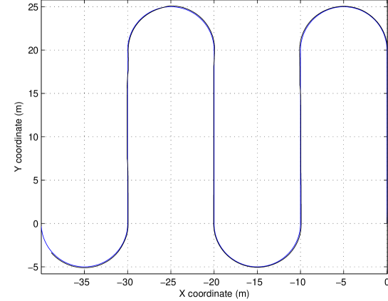
Figure 9.3: Simulations using the reduced actuation controller.

Figure 9.4: Offset error from the trajectory when using the reduced actuation controller.

Figure 9.5: Heading error obtained when using the reduced actuation controller.

Figure 9.6: Steering angle requested when using the reduced actuation controller.

Figure 9.7: Rate of change of the heading error obtained when using the reduced actuation controller.

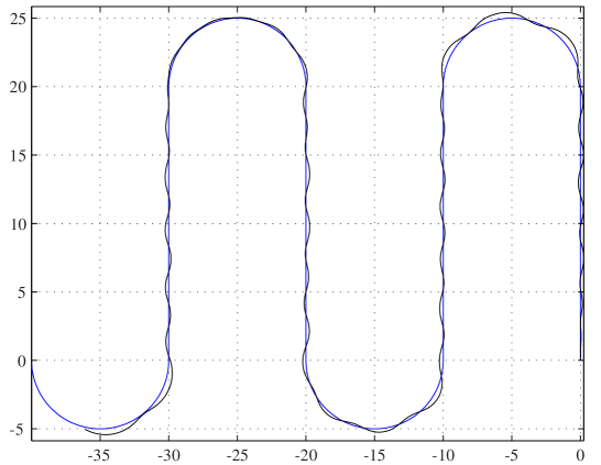
Figure 9.8: Simulations using the maximum actuation controller.

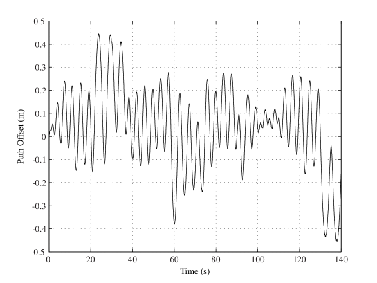
Figure 9.9: Offset error from the trajectory when using the maximum actuation controller.

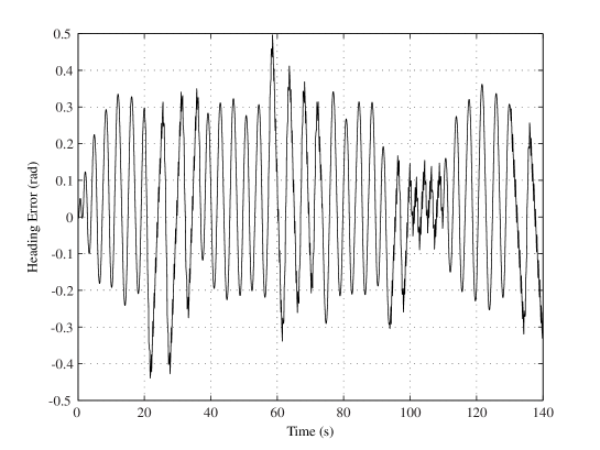
Figure 9.10: Heading error obtained when using the maximum actuation controller.

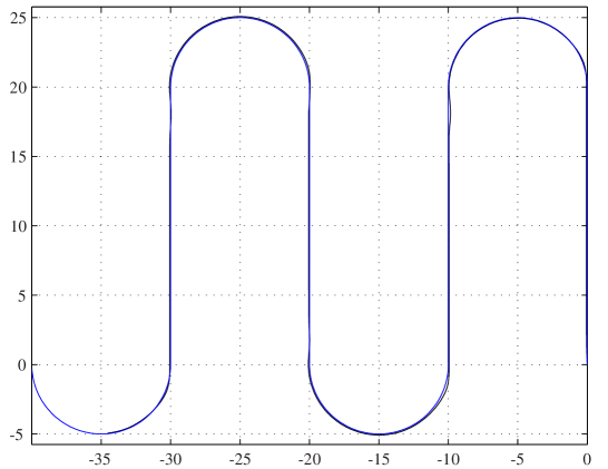
Figure 9.11: Simulations using the reduced actuation controller at high speed.

Figure 9.12: Performance of the reduced actuation controller at high speed.

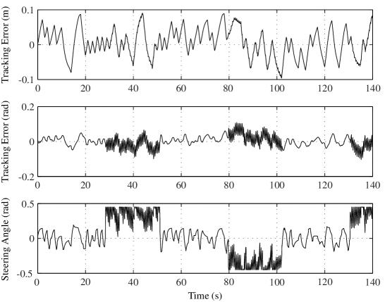
Figure 9.13: Offset errors and steering angle for the reduced actuation controller.

For a comparative study, the adaptive and predictive controller from [189] was chosen, which is among those with the best reported performances in off-road conditions. The simulation setup was basically borrowed from the previous subsection. The parameters of the adaptive controller were taken from [189]; the sideslip observer was not implemented to provide a more distilled comparison of the control laws themselves. The tractor wheelbase and steering dynamics were taken from [189], through the tractor speed was different; the speed is given in Table 9.4.

$v_{rw}$	$0.7ms^{-1}$
$\delta_{max}$	$0.7rad$
$L$	$2.75m$

$\mu$	$1.1rad$
$\Delta$	$0.2m$

$\sigma$	$0.5m$
$\underline{\varkappa}$	$0.01m^{-1}$

Table 9.4: Control parameters used during comparison test.

The two compared laws were tested against identical sequences of random slip parameters and sensor noises; $1000$ sequences were randomly generated and used in respective tests. Since the main concern of this chapter is about systematic occasional degradation of the tracking accuracy, the maximal spatial deviation from the reference path was chosen as the basic performance index for a given test. However, the root mean square (RMS) deviation was also taken into account. The diagrams in Figs. 9.14 and 9.15 show the number of tests (the vertical axis) with a given value of the performance index (the horizontal axis). It follows that the proposed controller provides $\approx 50\%$ of performance improvement on average, at least in the considered specific circumstances.

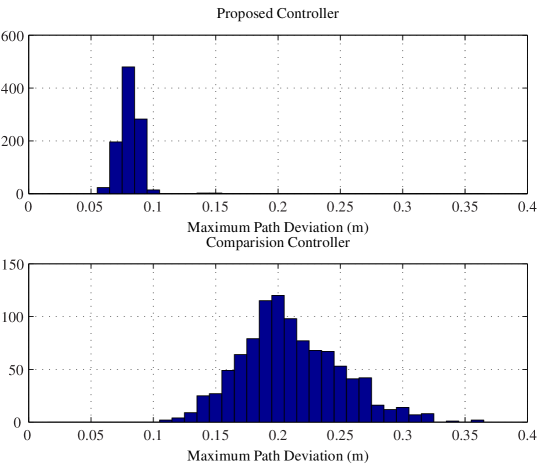
Figure 9.14: Comparative distribution of the maximal path deviation.

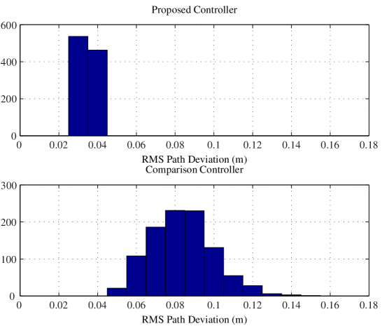
Figure 9.15: Comparative distribution of RMS path deviation.

9.8 Specifications of the Agricultural Vehicle

The controller was implemented on a fully autonomous compact agricultural tractor (see Fig. 9.16) developed at the University of New South Wales, Sydney, Australia. The tractor is fully custom instrumented and automated with the integration of a complete sensor suite and the accompanying software [81]. The base tractor was a John Deere 4210 Compact Utility Tractor [144].

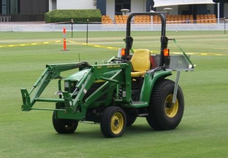
Figure 9.16: Autonomous tractor used for testing.

The control inputs to the tractor are the steering control signal and the propulsion control signal. The tractor’s propulsion system is driven by a hydrostatic transmission system, which allows the control of the speed through the control of its swash plate. The swash plate can be controlled through electronic means by directly applying the required voltage by interfacing to the built-in computer of the tractor. This facilitated a non-invasive means of controlling the vehicle speed. Two separate analog voltages, generated by the on-board computer (note that the built-in and on-board are two different computers), one for forward motion and another for reverse motion are used to control the forward and reverse speeds of the tractor. These two voltage channels correspond to the forward pedal and reverse pedal on the tractor. All other logic to take care of unacceptable scenarios such as both pedals being pressed at the same time or a pedal voltage exceeding its range are provided by the built-in computer of the tractor.

The automation of the steering however did not have the same ease of interfacing. Hence it was necessary to mount an additional actuator on the steering system. There was no positive coupling between the steered position of the wheels and the steering column angular position. Hence the mounting of a separate steering sensor was necessary. A non-linear relationship exists between the steering sensor position and the actual steered angle of the front wheels. A standard well tuned PI controller was implemented to control the steering. The desired steering is specified as the desired steering sensor position. Such a command can easily be generated to correspond a desired steered angle through a simple table look-up. The steering control system operates very well with a speed of response an order higher than the speed of response of the tractor motion.

Within limits (as determined by the manually controlled gear position), the speed of the tractor can be automatically controlled. The speed is obtained by averaging the rate of change of the encoder counts of the left and right hand rear wheel encoders. The rear wheels have an external diameter of 0.9 m. and the encoders generate 40000 counts per revolution. The on-board computer’s time stamp is used to calculate the actual speed in m/s.

9.8.1 Safety Subsystem

The safety subsystem is centered around the built-in computer’s halt mode that is wired to the seat switch. A simple re-triggerable one shot timer circuit mimics the seat switch signal, also known as the watch-dog signal, and when active selects the propulsion signals generated by the on-board computer instead of those generated by the pedals. The re-triggering of the timer must take place every 128 ms. or less, or else the watchdog signal will become inactive thereby switching all propulsion signals to the manual pedals. This requires the pedals to be pressed afresh to effect motion. If a pedal is not pressed or a driver is not present the tractor will be halted.

The control software is written in such a manner that if any of the critical software modules fail then the watchdog will be disabled. In addition an operator at the remote console may also choose to disable the watchdog signal.

9.8.2 Sensors

The tractor is equipped with a rich set of sensors. To measure its global position and orientation two GPS systems, both with 2 cm. RTK accuracy are available. Other sensors include an encoder each for the two rear wheels and a steering position sensor sensing the displacement of the steering system’s power cylinder. For communication between individual on-board components and the remote station outside the tractor, an Ethernet network is established and connected to an access point with a high gain antenna capable of 300m line-of-sight Wi-Fi communication.

9.8.3 Software

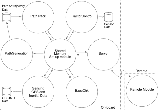
Figure 9.17: Software architecture.

A complete suite of software is put in place to take care of a variety of tasks. In addition to the on-board software modules, an additional module must run on a remote client. The data communication between the external client and the tractor’s on-board computer takes place via the earlier mentioned Wi-Fi network. The remote module predominantly control the watchdog signal in addition to the mode selection and remote control.

The software modules are shown in Fig. 9.17. Each circle represents a software module. Each link shows the data flow and the cylinders represent disk storage. The mode of operation of the tractor is chosen by the remote module through buttons on a joystick attached to the remote computer. The tractor can operate in one of three modes, (i) Path generation, (ii) Remote control and (iii) Autonomous control. Depending on the mode of operation various different software modules move onto the critical path. Based on the mode chosen the ExecChk module sequentially executes the required modules and monitors the live execution of all required modules adhering to the stipulated precedence. If any of the critical modules fail, the ExecChk module will initiate a shutdown. If the ExecChk itself fails, it will be detected by all other modules. In that situation, the TractorControl module will disable the watchdog signal. As an additional safety measure, the human operator stands guard of the watchdog signal at the remote station.

The PathGen module can generate a path of a predefined shape to align with the tractor’s current position and orientation. Obviously, for this to function the GPS readings must be available hence the GPS module must run before PathGen can be run. The SharedMem module facilitates data exchange between modules. The Server module maintain contact with the remote module and receives the mode select, watchdog signal and remote control commands. Sensing module acquires GPS and inertial data. Two separate sub-modules, one for GPS and one for the IMU are used within it due to their different data rates. The PathTrack module executes high level control algorithms. The TractorControl module carries out the low level control of the steering and propulsion while recording all low level sensor data.

9.9 Experiments

The dimensions of the experimental test trajectory were identical to the simulated scenario. The controller parameters for the experiment are shown in Table 9.5. The average speed of the tractor during the test was approximately $1.9km/h$. No filtering was done on the raw GPS measurements, which is acceptable due the high noise resistance of sliding mode control laws (the main type of error observed in the results is not attributable to random noise, but rather systematic offsets). The GPS receivers were evenly and equally spaced $0.230m$ behind the center of the rear axle, and the position and orientation of the rear axle was calculated directly based on this assumption.

The steering angle requested by the controller was used as the set-point for the steering controller specified in the previous section. The steering dynamics can be approximated by a rate limit, and while it was not accurately characterized a full transition of the steering between the steering limits was observed to take up to one second (dependent on vehicle speed). The mismatch between the actual steering dynamics and those assumed during the the theoretical development were found to not cause malfunction of the control system provided the tractor speed was not too large – for lower speeds, the delay in changing the steering angle has a lesser effect on the tractors state. More information about possible solutions to this problem are discussed in [83].

The results of the tractor test are shown in Figures 9.18, 9.19, 9.20 and 9.21, where it may be seen the tractor behaved as expected. In Fig. 9.21, the actual steering angle of the tractor is shown. It follows that the system operates near the mechanical steering angle limit, which is approximately equal to $0.6rad$.

The highest measured path offset error obtained was approximately $0.4m$, whereas the RMS error was $0.3199m$ and the RMS heading error was $0.2918rad$. There are some systematic errors when tracking straight path segments, and these are most likely caused by systematic errors in the measurement system. They could likely be eliminated by introducing some type of adaptive observer, however that is outside the scope of this chapter.

$\delta_{max}$	$0.5rad$
$L$	$1.69m$
$\mu$	$0.3rad$

$\Delta$	$0.15m$
$\sigma$	$0.5m$
$\underline{\varkappa}$	$0.05m^{-1}$

Table 9.5: Control parameters used for experiments.

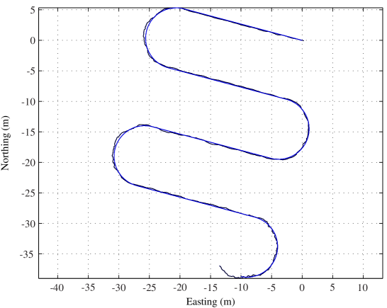
Figure 9.18: Trajectory obtained during the experiment.

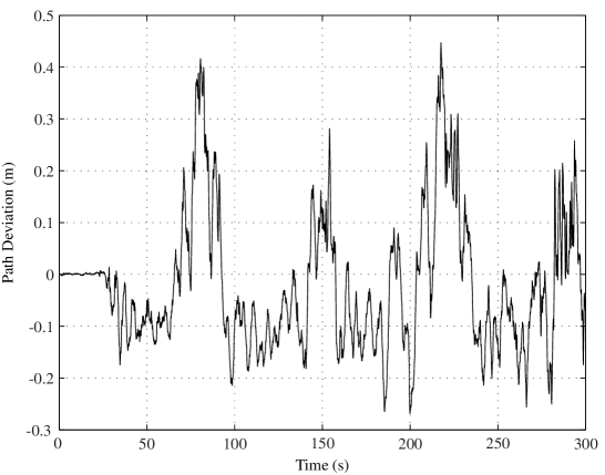
Figure 9.19: Path offset error obtained during the experiment.

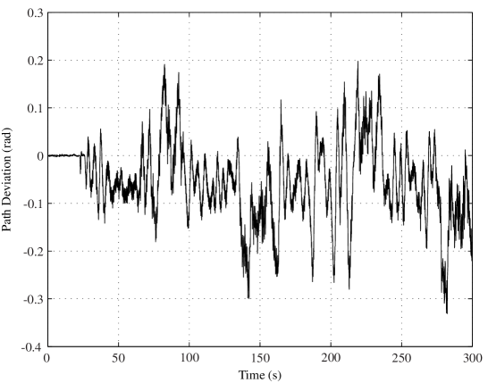
Figure 9.20: Heading error obtained during the experiment.

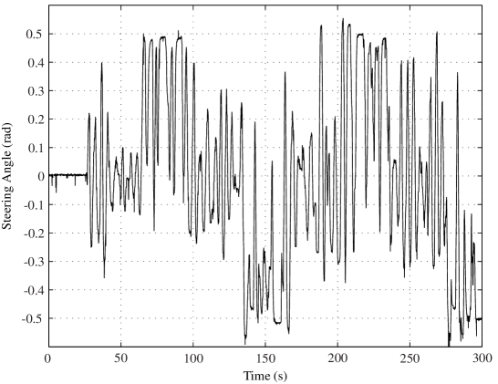
Figure 9.21: Actual steering angle of the tractor obtained during the experiment.

The experiment was undertaken on a very rough field, with the amplitude of undulation up to $15.0cm$. Though direct comparison with other controllers under similar circumstances is highly troublesome since every ”rough” field has its own individual features (which can be hardly described and reproduced in details), the observed tracking error is comparable with the best results reported in the literature.

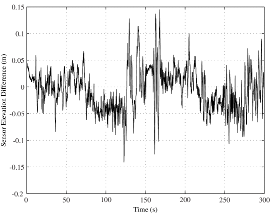
Figure 9.22: Difference in measured elevation between the two GPS sensors.

9.10 Summary

Two approaches for control of farm tractors in the presence of slippage are presented. One of them uses maximal actuation of the vehicle, whereas fluctuation of the control input is reduced with the aid of a smooth nonlinear control law for the other. Simulation studies showed that the nonlinear controller produced more stable trajectories with lower control efforts as compared to the pure sliding mode controller. Experiments were also carried out on a real agricultural vehicle, which confirmed the real world viability of the proposed control system.

Chapter 10 Boundary Following using Minimal Information

The boundary following method proposed in Chapt. 4 relies on numerous obstacle detections in order to successfully track the boundary of an obstacle. In this chapter, an alternative method is proposed, which is based on only the distance along and the reflection angle of the ray perpendicular to the vehicle centerline. Such a situation holds if the measurements are supplied by several range sensors rigidly mounted to the vehicle body at nearly right angles from its centerline, or by a single sensor scanning a similarly narrow sector. This perception scheme is used in some applications to reduce the complexity, cost, weight, and energy consumption of the sensor system and to minimize detrimental effects of mechanical external disturbances on the measurements.

This approach retains many of the advantages of the method proposed in Chapt. 4, such as provably correct behaviour, and no requirement for measurement of the boundary curvature. The main difference is that a equidistant curve from the boundary is tracked at constant speed, whereas the method in Chapt. 4 exhibits no fixed speed and offset from the boundary (which may make it unsuitable for certain applications). In addition, the method proposed in this chapter has very low computational requirements, and can be expressed as a simple sliding mode control law. The main disadvantage is that global assumptions are present which place bounds on the obstacle curvature (however these are unavoidable given the reduced amount of information available). Also, deficit of sensor data makes most of known navigation solutions inapplicable. This gives rise to special challenges, like inability to detect a threat of head-on collision in certain situations (see Fig. 10.3).

This chapter proposes a novel sliding-mode navigation strategy that does not employ curvature estimates and homogeneously handles both concavities and convexities of the followed boundary, as well as transitions between them. This strategy asymptotically steers the vehicle to the pre-specified distance to the boundary and afterwards ensures stable maintenance of this distance. In addition, mathematically rigorous justification results for non-local convergence of the proposed strategy are available. In doing so, possible abrupt jumps of the sensor readings are taken into account. Furthermore, much attention is given to revealing requirements to the global geometry of the boundary that make it possible to avoid front-end collisions with it based on only side view sensors, thus making extra front-view sensors superfluous. The convergence and performance of the proposed navigation and guidance law are confirmed by computer simulations and real world tests with a Pioneer P3-DX robot, equipped with a SICK LMS-200 LiDAR sensor.

All proofs of mathematical statements are omitted here; they are available in the original manuscript [222].

The body of this chapter is organized as follows. In Sec. 10.1 the problem is formally defined, and in Sec. 10.2 the main assumptions are described. A summary of the main results are in Sec. 10.3. Simulations and experiments are presented in Secs. 10.4 and 10.5. Finally, brief conclusions are given in Sec. 10.6.

10.1 Problem Statement

A Dubins-type vehicle travels in the plane with the constant speed $v$. It is controlled by the angular velocity $u$ limited by a given constant $\overline{u}$. There also is a domain $D$ with a smooth boundary $\partial D$ in the plane. The objective is to drive the vehicle over the equidistant curve of the domain $D$ separated from it by the pre-specified distance $d_{0}$ (see Fig. 10.1(a)). The vehicle is equipped with a narrow-aperture range sensor directed perpendicularly to the vehicle centerline and to the left. This sensor provides the distance $d$ from the vehicle to the nearest point of $D$ in the sensed direction (see Fig. 10.1(b)).

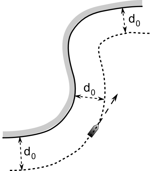
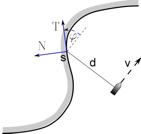
Figure 10.1: (a) Motion over the equidistant curve; (b) Vehicle with a rigidly mounted range sensor.

The scan within the aperture and processing of the collected data provides the vehicle with access to the angle $\varphi$ from its forward centerline to the tangential direction of the boundary at the reflection point. Whenever the sensor does not detect the obstacle, $d:=\infty,\varphi:=0$.

Apart from stable maintenance of the motion over the equidistant curve, it is required to ensure transition to this motion from a given initial state. In doing so, the vehicle must not collide with the boundary $\partial D$. The distance from the boundary if defined as follows:

$$\text{\bf dist}\,[r,D]:=\min_{r^{\prime}\in D}\|r-r^{\prime}\|$$ (10.1)

The distance from the vehicle location $r$ to the boundary should constantly exceed the given safety margin $d_{-}<d_{0}$.

The kinematics of the considered vehicles are classically described by the following equations:

$$\begin{array}[]{l}\dot{x}=v\cos\theta,\\ \dot{y}=v\sin\theta,\par\par\end{array},\quad\dot{\theta}=u\in[-\overline{u},\overline{u}],\quad\begin{array}[]{l}\boldsymbol{r}(0)=\boldsymbol{r}_{0}\not\in D\\ \theta(0)=\theta_{0}\end{array}.$$ (10.2)

Here $x,y$ are the coordinates of the vehicle in the Cartesian world frame, whereas $\theta$ gives its orientation, the angular velocity $u$ is the control parameter (see Fig. 10.2(a)). (The set of initial states $\boldsymbol{r}_{0}\not\in D$ for which the problem has a solution will be specified later on in Theorem 10.3.1.)

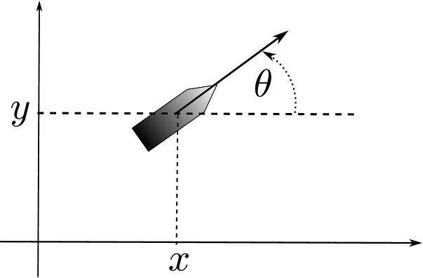
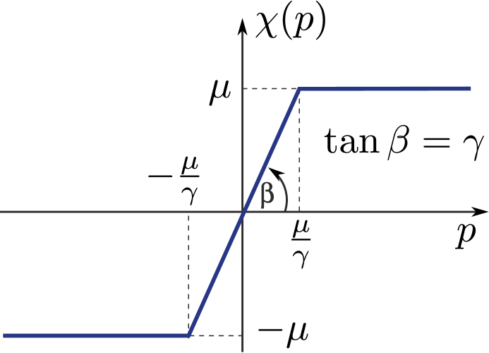
Figure 10.2: (a) Planar vehicle; (b) Linear function with saturation.

In the case at hand, the minimal turning radius is given by:

$$R=v/\overline{u}.$$ (10.3)

In this chapter, the following navigation law is examined:

$$u=\left\{\begin{array}[]{l}-\overline{u}\;\text{if}\;S:=\varphi+\chi[d-d_{0}]\leq 0\\ u_{+}:=\min\left\{\overline{u};vd^{-1}\right\}\;\text{if}\;S>0\end{array}\right..$$ (10.4)

Here $\chi(\cdot)$ is a linear function with saturation:

$$\chi(p):=\begin{cases}\gamma p&\text{if}\;|p|\leq\mu/\gamma\\ \text{\bf sgn}(p)\mu&\text{otherwise}\end{cases}.$$ (10.5)

The gain coefficient $\gamma>0$ and the saturation level $\mu\in\left(0,\frac{\pi}{2}\right)$ are design parameters (see Fig. 10.2(b)).

10.2 Main Assumptions

For the control objective to be achievable, the vehicle should be capable of tracking the $d_{0}$-equidistant curve of the boundary $\partial D$. However this is impossible if this curve contains cusp singularities, so far as any path of the unicycle Eq.(10.2) is everywhere smooth. Such singularities are typically born whenever the boundary contains concavities and the required distance $d_{0}$ exceeds the critical value, which is equal to the minimal curvature radius of the concavity parts of the boundary [15]. Moreover, even if there are no singularities, the equidistant curve should not be much contorted since the robot is able to trace only curves whose curvature radius exceeds Eq.(10.3). These observations are detailed in the conditions necessary for the $d_{0}$-equidistant curve to be trackable by the robot that are given by Lemmas 3.1 and 3.2 from [230]. Being slightly enhanced by putting the uniformly strict inequality sign in place of the non-strict one, they come to the following nearly unavoidable assumption:

Assumption 10.2.1

The following inequalities hold:

$$R_{\varkappa}^{+}(D):=\inf_{r\in\partial D:\varkappa(r)>0}R_{\varkappa}>R-d_{0},\quad R_{\varkappa}^{-}(D):=\inf_{r\in\partial D:\varkappa(r)<0}R_{\varkappa}>d_{0}+R$$ (10.6)

and the curvature is bounded $K:=\displaystyle{\sup_{r\in\partial D}}|\varkappa(r)|<\infty$.

Here $\varkappa=\varkappa(r)$ is the signed curvature of $\partial D$ at $r$, $R_{\varkappa}:=|\varkappa|^{-1}$ is the curvature radius, and $\inf$ over the empty set is defined to be $+\infty$. The signed curvature is non-negative on convexities of the boundary and negative on concavities.

As is illustrated in Fig. 10.3, the sensor system of the vehicle is deficient in capability of on-line detection of head-on collisions with the domain $D$. In the absence of extra forward-view sensors, a partial remedy may be systematic full turns to accomplish environment mapping within the entire vicinity of the vehicle given by the sensor range, which however consumes extra resources and may be unacceptable. If no special measures are taken to explore the forward direction, collisions can be excluded only due to special geometric properties of the obstacle $D$. They should guarantee a certain amount of free forward space on the basis of circumstances sensible in the side direction. These guarantees should cover the entire operational zone including the transient.

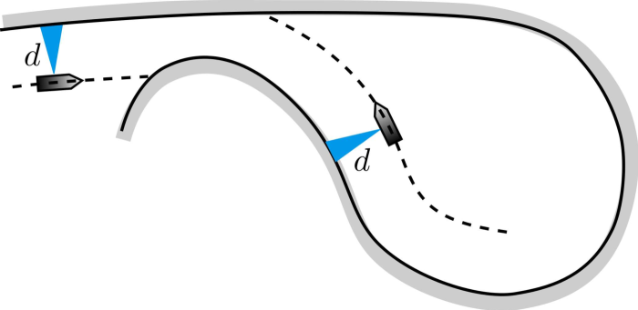
Figure 10.3: Insufficiency of the side sensor to ensure safety.

Local guarantees of such a kind are given by Eq.(10.6). To highlight this, the outer normal ray to $\partial D$ (rooted at $r\in\partial D$) is denote by $\mathscr{N}(r)$. Also, the point of $\mathscr{N}(r)$ at the distance $L$ from $r$ is denoted by $r(L)$. Then the second inequality from Eq.(10.6) implies that some piece $\partial_{s}D$ of $\partial D$ surrounding $r$ does not intersect the open disk of the radius $d_{0}+R$ centered at $r(d_{0}+R)$ [15], as is illustrated in Fig. 10.4. In turn, this implies that first, the smaller disk of the radius $R$ centered at $r(d_{0}+R)$ is separated from $\partial_{s}D$ by a distance of not less than $d_{0}>d_{-}$ and second, the smaller open disk $\mathfrak{D}(r,d_{0})$ of the radius $d_{0}$ centered at $r(d_{0})$ does not intersect $\partial_{s}D$. Now these guarantees are extended on the entire boundary and operational zone, which is assumed to be upper limited $d\leq d_{\ast}$ by a constant $d_{\ast}$:

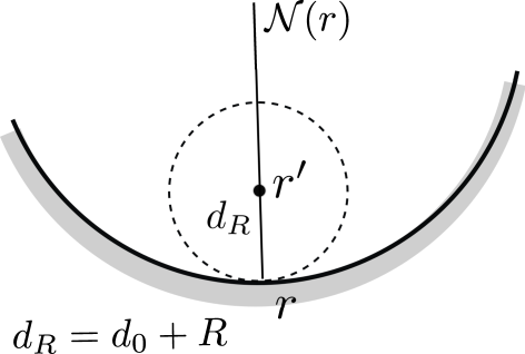
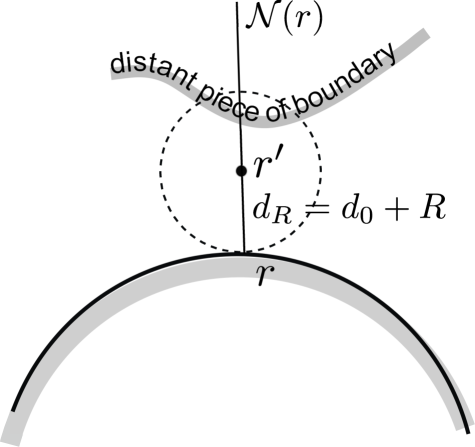
Figure 10.4: A disk free of collision with the local part of the boundary.

Assumption 10.2.2

The following two claims hold:

1. For any $r\in\partial D$, the open disk $\mathfrak{D}(r,d_{0})$ is disjoint with the entire boundary $\partial D$;

2. There exist $d_{\ast}>d_{0}$ and $\eta>0$ such that for any $r\in\partial D$, the set $Q(r,0)$ introduced by Fig. 10.5(a) is separated from the boundary $\partial D$ by a distance of not less than $d_{-}+\eta$; see Fig. 10.5(b).

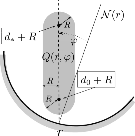
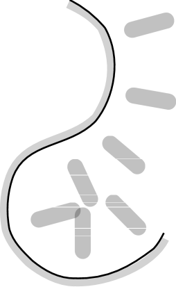
Figure 10.5: (a) The set $Q(r,\varphi)$; (b) Assumption 10.2.2.

It follows from Fig. 10.5(a) that $d_{-}+\eta<d_{0}$.

Finally it is assumed that the distance to $D$ is locally controllable when operating at the safety margin $d_{-}$: it can be maintained constant, increased, and decreased by selecting respective controls. As was shown in [230], this is equivalent to the following enhancement of the first inequality from Eq.(10.6):

Assumption 10.2.3

The following inequality holds:

$$R_{\varkappa}^{+}(D)+d_{-}>R.$$ (10.7)

The similar condition $R_{\varkappa}^{-}(D)>d_{-}+R$ for the concavity parts $\varkappa<0$ of the boundary follows from the second inequality in Eq.(10.6) since $d_{0}>d_{-}$.

Due to Eq.(10.6), Eq.(10.7), there exists $\mu\in\left(0,\frac{\pi}{2}\right)$ such that:

$$R_{\varkappa}^{+}(D)\cos\mu+d_{-}>R,$$ (10.8)

$$R_{\varkappa}^{-}(D)\cos\mu>R+d_{0}.$$ (10.9)

The parameter $\eta_{\ast}\in(0,\eta)$ may be picked, where $\eta$ is taken from (ii) of Assumption 10.2.2, and by decreasing $\mu$ if necessary, ensure the following property, which is possible thanks to Assumption 10.2.2:

Property 10.2.1

For any $r\in\partial D$ and $\varphi\in[-\mu,\mu]$, the following two claims hold:

1. For any point $r^{\prime}$ such that $\|r^{\prime}-r\|\leq d_{0}$ and the angle subtended by $r^{\prime}-r$ and the normal $\mathscr{N}(r)$ equals $\varphi$,

   • the straight line segment with the end-points $r$ and $r^{\prime}$ has only one point $r$ in common with $\partial D$;

   • the distance from $r^{\prime}$ to $\partial D$ is no less than $d_{-}$ provided that $\|r^{\prime}-r\|\geq d_{-}+\eta_{\ast}$;

2. the set $Q(r,\varphi)$ is separated from the boundary $\partial D$ by a distance of not less than $d_{-}+\eta_{\ast}$.

Finally, the variable $[s]_{+}$ is set to $\max\{s,0\}$, and $\gamma$ is picked so that:

$$\gamma<\frac{R_{\varkappa}^{+}(D)\cos\mu-[R-d_{-}]_{+}}{R_{\varkappa}^{+}(D)[R-d_{-}]_{+}\sin\mu}\;\text{if}\;R>d_{-},$$ (10.10a)

$$\gamma<\frac{R_{\varkappa}^{-}(D)\cos\mu-(R+d_{0})}{(R+d_{0})R_{\varkappa}^{-}(D)\sin\mu},$$ (10.10b)

$$\gamma<\frac{\cos\mu}{(R+d_{0})\sin\mu}.$$ (10.10c)

This choice is possible, since the right-hand sides of all inequalities are positive due to Eq.(10.8) and Eq.(10.9).

If the boundary $\partial D$ is compact, inequalities Eq.(10.6)–Eq.(10.10b) can be checked in the point-wise fashion. In doing so, any inequality involving $R_{\varkappa}^{+}(D)$ should be checked at any point $r\in\partial D$ of convexity $\varkappa(r)>0$ with substituting $R_{\varkappa}(r)$ in place of $R_{\varkappa}^{+}(D)$. Similarly, any inequality involving $R_{\varkappa}^{-}(D)$ should be checked at any point $r\in\partial D$ of concavity $\varkappa(r)<0$ with substituting $R_{\varkappa}(r)$ in place of $R_{\varkappa}^{-}(D)$.

10.3 Summary of Main Results

When examining convergence of the control law, it is assumed that the initial state is in the set $\mathscr{V}$ of all states $r\not\in D,\theta$ for which the domain is visible. Let $d(r,\theta)$ denote the corresponding measurement $d$.

The set $\mathfrak{C}$ of initial states $r,\theta$ from which convergence to the required equidistant curve can be theoretically guaranteed is composed of three parts $\mathfrak{C}_{0},\mathfrak{C}_{-}$, and $\mathfrak{C}_{+}$. They contain initial states with $S=0,S<0$, and $S>0$, respectively, where $S$ is defined in Eq.(10.4):

$$\mathfrak{C}_{0}:=\Big{\{}(r,\theta)\in\mathscr{V}:S=0\;\text{and}\;d_{-}+\eta_{\ast}\leq d\leq d_{\ast}\Big{\}}.$$ (10.11)

To introduce $\mathfrak{C}_{-}$, attention is first paid to the following:

Lemma 10.3.1

Under the control law Eq.(10.4), motion with $S<0$ necessarily terminates with arrival at $S=0$, provided that the vehicle does not collide with the domain $D$.

Let $C^{-}_{r,\theta}$ be the circle of radius Eq.(10.3) traced clockwise from the initial state $r,\theta$ and $(r_{\ast},\theta_{\ast})$ be the first position on this circle that either belongs to $D$ or is such that $S=0$. By Lemma 10.3.1, this position does exist. Let also $\widehat{C}^{-}_{r,\theta}$ denote the arc of $C^{-}_{r,\theta}$ between these two positions, and $\textbf{dist}(A,B):=\inf_{r\in A,r^{\prime}\in B}\|r-r^{\prime}\|$ denote the distance between the sets $A$ and $B$. The second part of the set $\mathfrak{C}$ is given by:

$$\mathfrak{C}_{-}:=\Big{\{}(r,\theta)\in\mathscr{V}:S<0,\quad\textbf{dist}[\widehat{C}^{-}_{r,\theta},D]\geq d_{-},\\ \text{and}\quad d(r_{\ast},\theta_{\ast})\geq d_{-}+\eta_{\ast}\Big{\}}.$$ (10.12)

Introduction of the last part $\mathfrak{C}_{+}$ is prefaced by the following:

Lemma 10.3.2

Under the control law Eq.(10.4) and for initial states with $S>0$, there may be the following three scenarios:

1. With maintaining $S>0$, the safety margin is violated;

2. With respecting the safety margin and maintaining $S>0$, the vehicle arrives at a position where the view of $D$ becomes obstructed by another part of $D$; at this moment, $S$ abruptly jumps down at a negative value;

3. With respecting the safety margin and maintaining both the view of $D$ unobstructed and $S>0$, the vehicle arrives at $S=0$.

While $S>0$, the vehicle moves counter-clockwise over the circle of the radius $d$ centered at the reflection point (which does not move) whenever $d>R$. Otherwise it moves with the maximal turning rate $\overline{u}$ over a circle of radius Eq.(10.3).

Finally the set $\mathfrak{C}_{+}$ is introduced, which contains all initial states $(r,\theta)\in\mathscr{V}$ for which the following claims hold:

• Scenario i) from Lemma 10.3.2 does not hold and $S(0)>0$;

• In the case ii) from Lemma 10.3.2, the vehicle arrives at a state from the set $\mathfrak{C}_{-}$ when $S$ becomes negatives

• In the case iii) from Lemma 10.3.2, the vehicle arrives at a state from the set $\mathfrak{C}_{0}$ when $S$ becomes zero.

Now the main result of the chapter may be stated:

Theorem 10.3.1

Let Assumptions 10.2.1–10.2.3 be true and in Eq.(10.4), the parameters be chosen so that Eq.(10.8)–Eq.(10.10c) and Property 10.2.1 hold. If the initial state lies in the set $\mathfrak{C}:=\mathfrak{C}_{0}\cup\mathfrak{C}_{-}\cup\mathfrak{C}_{+}$, the vehicle driven by the navigation and guidance law Eq.(10.4) does not lose track of the domain $D$, respects the safety margin, and asymptotically follows the boundary of $D$ at the required distance: $d(t)\to d_{0},\varphi(t)\to 0$ as $t\to\infty$.

10.4 Simulations

Simulations were performed using the perfect kinematic model of the vehicle Eq.(10.2). To estimate the angle $\varphi$, the tangent at the reflection point was approximated by the secant between this point and another point slightly in front; the angular separation between these points was $9$ deg. The control law was updated with the sampling period of $0.1s$. Other parameters used for simulation are shown in Table 10.1.

$\overline{u}$	$45.8deg/s$
$v$	$0.3m/s$
$\mu$	$57.3deg$

$\gamma$	$171.9deg/m$
$d_{0}$	$1.0m$

Table 10.1: Simulation parameters for fixed-sensor boundary following controller.

In the first simulation test, the domain $D$ fits the maneuverability of the robot: the minimal turning radius of the vehicle exceeds the radius required for perfectly tracking the boundary of $D$ with the requested margin $d_{0}$. Fig. 10.6 shows that after a short transient, the proposed control law provides a visibly perfect motion over the desired equidistant curve and successfully copes with both convexities and concavities of the obstacle, as well as with transitions from convexities to concavities and vice versa.

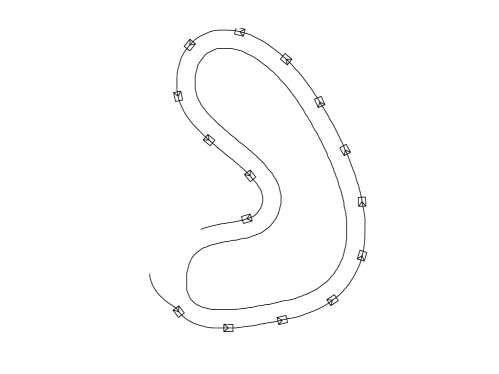
Figure 10.6: Simulations with a simple boundary.

Figs. 10.7 and 10.8 provide a closer look at the boundary following errors. After the transient is completed ($t\gtrapprox 18sec$), the error in the true distance to the obstacle Eq.(10.1) does not exceed $1cm$, whereas the error in the estimated angular discrepancy $\varphi$ between the tangent at the reflection point and the vehicle centerline does not exceed $12.6^{\circ}$. However, this good exactness proceeds from taking into account only the non-idealities that are due to control sampling and numerical evaluation of the relative tangent angle.

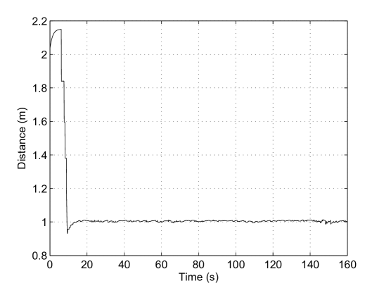
Figure 10.7: Distance to the obstacle during simulation.

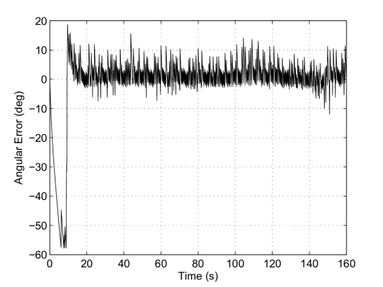
Figure 10.8: Estimated relative tangent angle $\varphi$ during simulation.

The second group of simulation tests provides deeper insights into the effects of real-live non-idealities on the performance of the closed-loop system. These tests were carried out in the previous scene with additionally taking into account sensor and actuator noises and un-modeled dynamics. To this end, a bounded random and uniformly distributed offset was added to every relevant quantity at each control update. Specifically, the noises added to $d$ and $\varphi$ were $0.3m$ and $17.2^{\circ}$, respectively; the noise added to the control signal was $11.5deg/s$, and the control signal was not allowed to change faster than $4rads^{-2}$. These are relatively large noises that would be unlikely met for typical modern sensors and actuators. The test was repeated several times, each with its own realization of the random noises. Ten typical results are depicted in Fig. 10.9. They show that the control objective is still achieved with the distance error $\leq 0.3m$. Since this is the accuracy of the distance sensor, the result seems to be more than satisfactory.

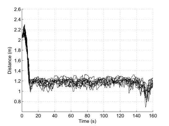
Figure 10.9: Distance to obstacle during simulations with actuator dynamics and sensor noises.

The purpose of the next test is to examine the performance of the algorithm in the case when the obstacle boundary $\partial D$ contains points where the vehicle is absolutely incapable of maintaining the required distance $d_{0}$ to $D$ because of the limited turning radius (see Fig. 10.10) – to move over the equidistant curve, the vehicle should turn sharper than feasible. Though the main theoretical results of the work are not concerned with this case, it may be hypothesized that if these points constitute only a small piece of the boundary, the overall behavior of the closed-loop system remains satisfactory. To verify this hypothesis and reveal details, the obstacle depicted in Fig. 10.11 is considered, for which concavities do contain the afore-mentioned points.

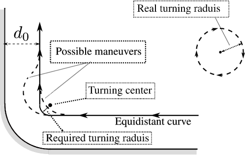
Figure 10.10: Unavoidable disturbance of the distance to $D$ because of the limited turning radius.

The related results are shown in Figs. 10.11, 10.12 and 10.13. All abrupt local both falls of the distance $d$ in Fig. 10.12 and deviations of the angle $\varphi$ from $0$ in Fig. 10.13 hold at $t\approx 90,130,190,300,340,400,490sec$ when the vehicle passes points where it is absolutely incapable to maintain the distance to $D$ at the level $d_{0}$. However, the algorithm demonstrates a good capability of quickly recovering after these unavoidable distance errors, and except for the related short periods of time and the initial transient, keeps the distance error within a very small bound of $1cm$ and always maintains the margin of safety at the level $\geq 0.3m$. This good overall performance is illustrated by Fig. 10.11, where the vehicle’s path looks like nearly perfect except for few very local violations of the required distance, with the most of them being hardly visible. The worst distance error is observed when passing the left upper concavity in Fig. 10.11. This concavity is similar to that from Fig. 10.10 – it is of the right-angle type. Such concavities are challenging for vehicles equipped with only side-view sensors. For example, when perfectly following the horizontal part of the equidistant curve from Fig. 10.10, the vehicle with side-view sensor is incapable to detect the need for turn until the reflection point leaves the flat part of the boundary. Even if the vehicle performs the sharpest turn after this, its forward advancement towards the vertical part of the boundary may be nearly equal to the minimal turning radius Eq.(10.3) (which holds if in Fig. 10.10, the ‘requested turning radius’ is close to $0$). For the vehicle examined in the simulation tests, the minimal turning radius amounts to $0.375m$. So theoretically the distance to the obstacle may be reduced to $1m-0.375m=0.625m$ when passing the above concavity. Practically it reduces to $\approx 0.3m$, where the difference is basically caused by errors in numerical evaluation of the tangent angle $\varphi$. Except for this troublesome concavity, the control law ensures the safety margin of $\geq 0.6m$ according to Fig. 10.12.

Figure 10.11: Simulation with a tight boundary.

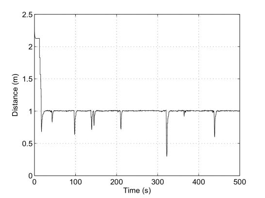
Figure 10.12: Distance to the obstacle during simulation.

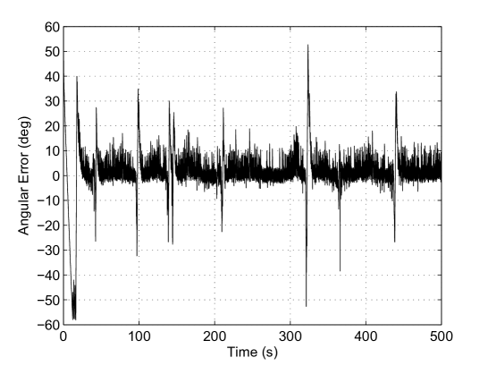
Figure 10.13: Estimated relative tangent angle $\varphi$ during simulation.

In this test like in the first one, only non-idealities related to control sampling and numerical evaluation of the relative tangent angle were taken into account. Simulations were also carried out to test the additional effect of un-modeled dynamics, sensor noise, and actuator noise on the performance of the closed-loop system in the environment from Fig. 10.11. All these phenomena were modeled like in the second group of simulations. Ten typical results corresponding to various realizations of the random noises are depicted in Fig. 10.14. Similarly to the second group of simulations, the distance accuracy degradation is approximately equal to the error of the distance sensor, which seems to be the fair price for using imperfect sensors. The vehicle still successfully follows the boundary without collision with the obstacle.

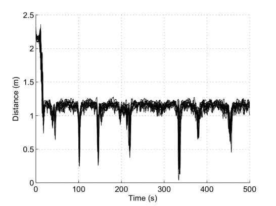
Figure 10.14: Distance to the obstacle during simulations with actuator dynamics and sensor noises.

The next series of simulation tests were aimed at illustration of the algorithm performance in environments with many obstacles. The objective of the algorithm is to follow the boundary of the selected obstacle $D_{0}$ despite presence of the others. According to the above discussion, it does follow the boundary provided that firstly, the view of $D_{0}$ is not obstructed and secondly, the assumptions of Theorem 10.3.1 are satisfied, in particular, the boundary of $D_{0}$ is everywhere smooth. The first requirement can be typically met by picking the desired distance of boundary following $d_{0}$ small enough as compared with spacing between obstacles. So the focus in the tests was on following boundaries with fractures (see Fig. 10.15).

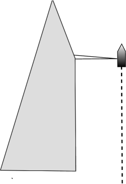
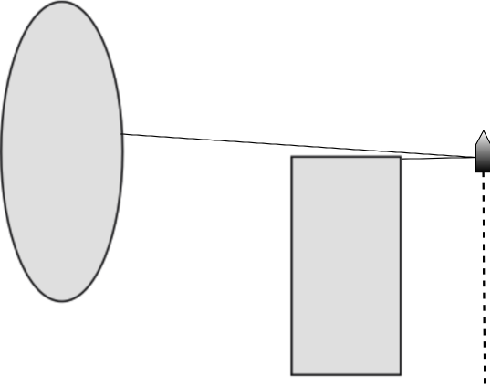
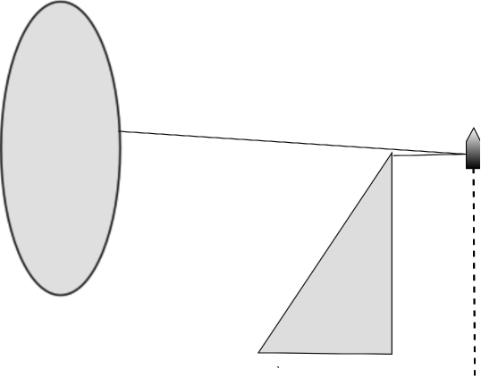
Figure 10.15: Following boundaries with fracture points.

At the fracture point, the tangent $T$ to the boundary and the angle $\varphi$ between $T$ and the vehicle centerline, which is used in the control law Eq.(10.4), are strictly speaking undefined. So the employed method to access $\varphi$ may be puzzled at fractures, with the outcome being dependent on the method. In these experiments, the tangent $T$ was approximated by the secant between the points $\boldsymbol{r}_{\ast}$ and $\boldsymbol{r}_{+}$ of incidence of the perpendicular ray $R_{\ast}$ and a ray $R_{+}$ slightly in front, respectively. When arriving at a fracture point, this method implies an abrupt increase of $\varphi$. Let for simplicity the vehicle perfectly follow the boundary $d\equiv d_{0},\varphi\equiv 0$ prior to this event. Then the angle becomes positive $\varphi>0$. By Eq.(10.4), this causes vehicle rotation about $\boldsymbol{r}_{\ast}$ at the distance $d_{0}$ from $\boldsymbol{r}_{\ast}$; see Fig. 10.16.

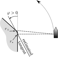
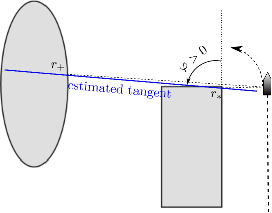
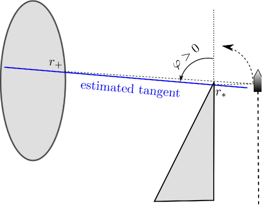
Figure 10.16: Rotation about $\boldsymbol{r}_{\ast}$.

This rough analysis gives a first evidence that the vehicle maintains following the boundary of the obstacle at hand, as is desired.

Figure 10.17: Following a fractured boundary in a cluttered environment.

Similar results with a slightly worse performance are obtained in the case where the ‘preceding’ ray $R_{+}$ is replaced by a ray $R_{-}$ slightly behind $R_{\ast}$, and the distance $d$ in the perpendicular direction is computed as $d:=\min\{d_{\ast},d_{-}\}$, where $d_{-}$ and $d_{\ast}$ are the distances along the respective rays; see Fig. 10.18. The idea to compute the distance to the nearest obstacle as the minimum of available distances along two close rays conforms to common sense. If it is illogically set to the maximum of them, the vehicle correctly passes obtuse fractures but for right and acute ones, starts circular motion about the farthest incidence point in accordance with Eq.(10.4), thus switching to a bypass of the competing obstacle; see Fig. 10.19.

Figure 10.18: Following a fractured boundary with the use of the ‘following’ ray $R_{-}$.

Figure 10.19: Following a fractured boundary in the case where illogically $d:=\max\{d_{\ast},d_{-}\}$.

Simulations were also carried out to compare the performance of the proposed navigation method with that from [158]. The latter algorithm employs the boundary curvature. By following [158], a geometric estimate of this curvature was used in these simulations. It results from drawing a circle through three boundary points detected by three close rays; the main perpendicular ray and two auxiliary rays on either side of the main one. The lengths to the boundary along every detection ray were corrupted by iid noises uniformly distributed over the very small interval $[-5mm,5mm]$. The same noises affected the two-point approximation of the tangent to the boundary for the control law proposed in this chapter. To enhance the difference, the both methods were equally challenged by not pre-filtering the noisy measurements. The simulation scenario was the obtuse corner from Fig. 10.17. The parameters of the controller from [158] were taken to be $\varkappa_{M}:=0.6;\varepsilon:=0.4;\varepsilon_{2}=0.2;\mu=1;\mu_{2}=5;\mu_{3}=5$, which meets the guidelines given in [158]. All simulation tests started at a common position, which corresponds to perfectly following the boundary at the required distance $d_{0}$. The tests were repeated $500$ times with individual realizations of the noises; for each test, the maximal (over the experiment) deviation from the desired distance to the boundary $\max_{t}|d(t)-d_{0}|$ was recorded.

The overall results are demonstrated by the histogram in Fig. 10.20, which shows the number of experiments with a given maximal deviation. The displayed better performance of the proposed method is presumably due to getting rid of the second derivative property (the boundary curvature) in the control law, which is particularly sensitive to both the distance measurement noises and violations of the boundary smoothness.

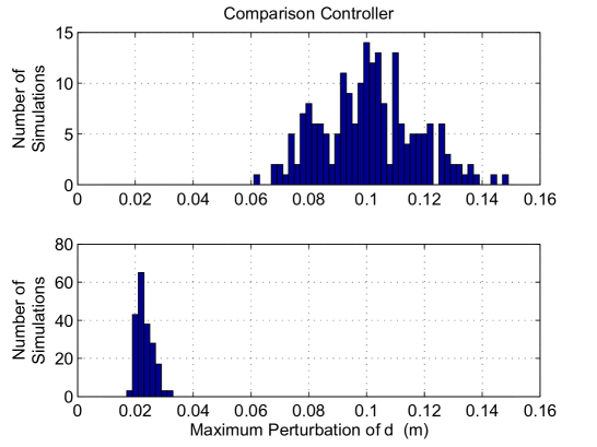
Figure 10.20: Distribution of the maximum distance error for two boundary following methods.

10.5 Experiments

Experiments were performed with a Pioneer P3-DX mobile robot, equipped with a SICK LMS-200 LiDAR device. The controller was slightly modified by continuous approximation of the nominal law Eq.(10.4):

$$u_{\text{act}}:=\text{\bf sgn}(u)\cdot\min\{|u|,\lambda|S|\}$$

Here $u$ is given by Eq.(10.4) and $\lambda$ is a tunable parameter; $\lambda=2$ in the experiments. Continuous approximation in a boundary layer is a common approach in practical implementation of discontinuous control laws [339, 84, 327], basically aimed at chattering elimination.

The control requested by the navigation law was forwarded as the desired steering input to the ARIA library associated with the robot (version 2.7.4). The control was updated at the rate of $0.1s$, and the angle between the two rays used to determine the secant that approximates the tangent to the obstacle boundary was set to be $10$ deg. The parameters used in testing are shown in Table 10.2.

$\overline{u}$	$28.6deg/s$
$v$	$0.2ms^{-1}$
$\mu$	$57.3deg$

$\gamma$	$171.9deg/m$
$d_{0}$	$0.5m$

Table 10.2: Experimental parameters for fixed-sensor boundary following controller.

The path obtained is shown in Fig. 10.21 and is captured by manually marking the position of the robot on the video frames. Both the video and Fig. 10.21 demonstrate that the robot behaves as expected, successfully circling the obstacle with both concavities and convexities without collision and with a safety margin $\geq 0.46cm$. The related tracking measurements are displayed in Figs. 10.22 and 10.23. As is seen in Fig. 10.22, the deviation of the distance measurement $d$ from the desired value $0.5m$ is always within the interval $[-4.0cm,+6.0cm]$ and moreover, is typically in $[-1.0cm,+3.0cm]$, except for several very short jumps out of this smaller range. However after these jumps, the vehicle quickly recovers. Except for the respective short periods of time, the distance error typically does not exceed $3.0cm$, with the dangerous deviation from the required distance towards the obstacle being no more than $1cm$. As is seen in Fig. 10.23, the estimate of the boundary relative tangential angle $\varphi$ is subject to a significant amount of noise. This is due to amplifying the noise in the distance measurement during numerical evaluation of $\varphi$ via approximation of the tangent by the secant between two close points of the boundary. This approximation also appeared to be sensitive to small angular perturbations accompanying the motion of the vehicle. Even with these detrimental effects, the controller has demonstrated the good ability to achieve the desired outcome.

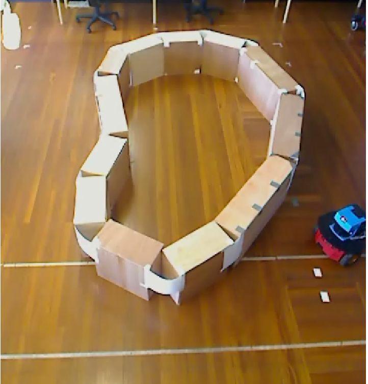
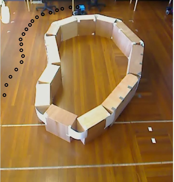
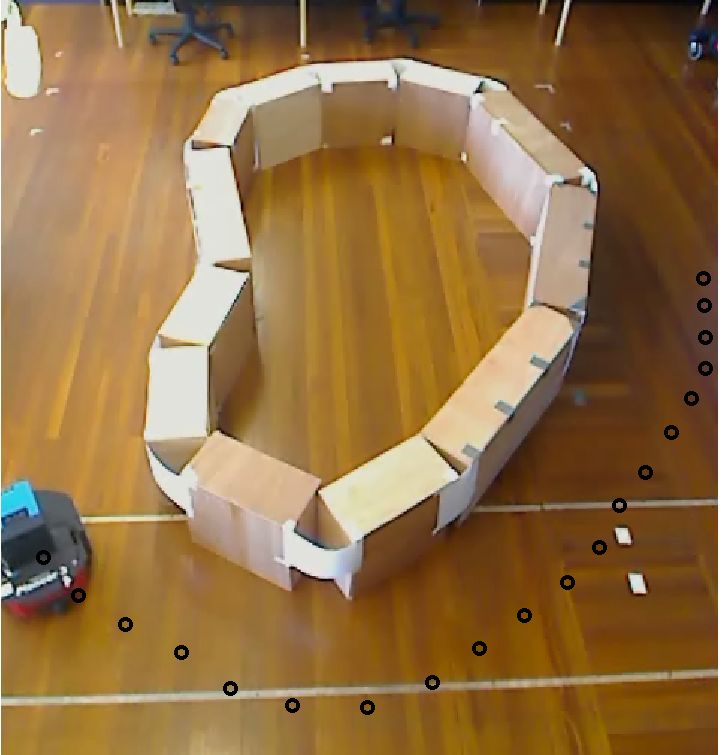
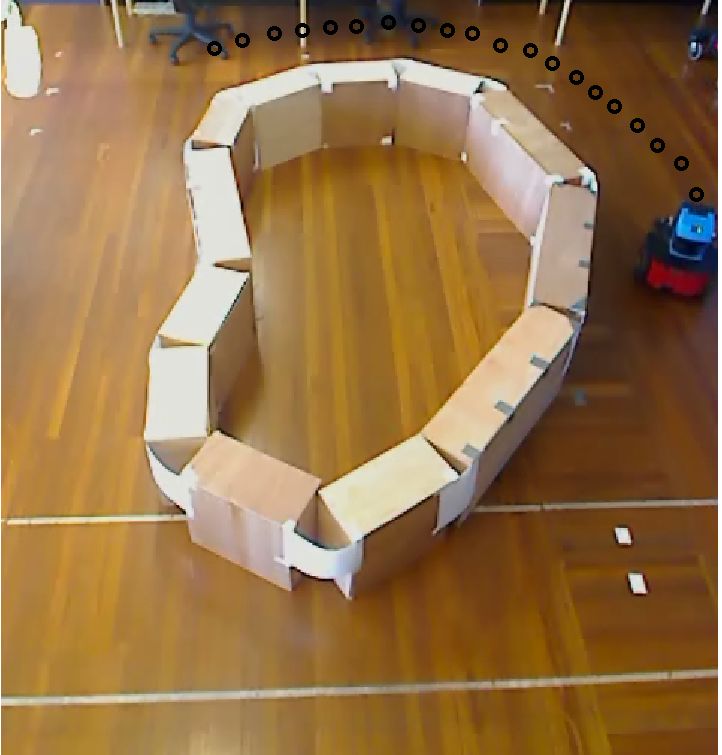
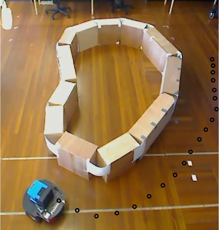
Figure 10.21: Sequence of images showing the experiment.

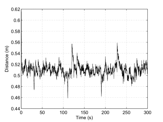
Figure 10.22: Distance measurement $d$ during the experiment.

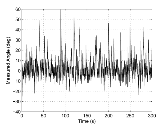
Figure 10.23: Estimate of the relative tangent angle $\varphi$ during the experiment.

The objective of the second experiment was to test the effect of a thin obstacle for which the obstacle curvature assumptions adopted in the theoretical part of the chapter are heavily violated at the end of the obstacle. The results are shown in Figs. 10.24–10.26. In accordance with explanatory remarks on Fig. 10.17, passing the obstacle end is accompanied with detection of a different and farther obstacle, as can be seen in Fig. 10.25, which displays the farthest distance detected within the employed narrow beam of detection rays for illustration purposes. However due to the reasons disclosed at the end of Sec. 10.4, the robot successfully copes with the thin obstacle and behaves as expected.

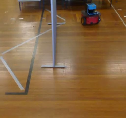
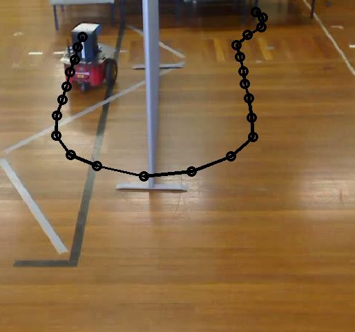
Figure 10.24: Sequence of images showing the experiment (thin obstacle).

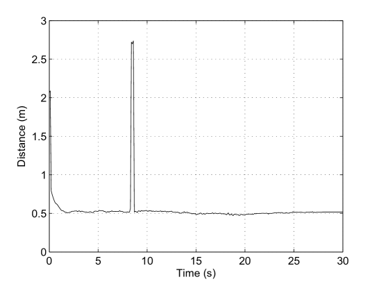
Figure 10.25: Distance measurement during the experiment with a thin obstacle.

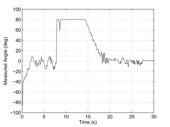
Figure 10.26: Estimate of the relative tangent angle $\varphi$ during the experiment with a thin obstacle.

Figs. 10.27–10.29 present typical results of experiments in more cluttered environments. As compared with the previous experiments, the speed of the robot was reduced to $0.05ms^{-1}$ to make its minimal turning radius Eq.(10.3) smaller less than spacing between the obstacles. It can be seen that the robot correctly navigates around the selected obstacle despite the presence of the others.

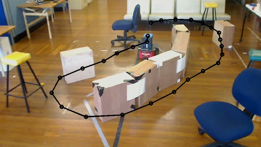
Figure 10.27: Sequence of images showing the experiment (cluttered environment).

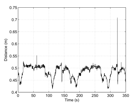
Figure 10.28: Distance measurement during the experiment in the cluttered environment.

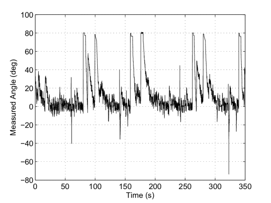
Figure 10.29: Estimate of the relative tangent angle $\varphi$ during the experiment in the cluttered environment.

10.6 Summary

In this chapter, a novel approach for navigating an unmanned unicycle-like vehicle along an obstacle boundary is proposed. It deals with the situation where knowledge of the boundary is related to a single detection ray directed perpendicularly to the vehicle centerline. A sliding mode navigation law is proposed, which is able to drive the vehicle at a fixed distance from this boundary. Computer simulations and experimental results with a real wheeled robot confirm the viability of the method.

Chapter 11 Extremum Seeking Navigation in a Scalar Field

In this chapter, a method for driving a vehicle to the maximal point of a scalar environmental field is proposed. The main advantage of the proposed method is that it requires estimation of neither the spatial or temporal derivatives of the field value, yet convergence to the maximal point can be proven under certain assumptions. Simulations and experimental results are given to confirm the viability of the proposed method.

11.1 Introduction

The chapter addresses the problem of driving a single robot to the maximizer of an unknown scalar environmental field. For example, this may be thermal, magnetic, electric, or optical field; or concentration of a chemical, physical, or biological agent. Some examples of missions where this problem is of interest include environmental studies, geological exploration, detecting and localizing the source of hazardous chemical, vapor, radiation emission, or also the pursuit of a moving target. In the last case, the objective is to approach the target and follow it with a pre-specified margin. Apart from source seeking/localizing [360, 264, 61], this problem is often referred to as gradient climbing/ascent [253, 35, 17, 46], which highlights the common kinematic control paradigm – try to align the velocity vector of the robot with the field gradient.

Recent surveys on extremum seeking control methods and algorithms are available [164, 76]. A good deal of related research was concerned with gradient climbing based on direct on-line gradient estimation. This approach is especially beneficial for mobile sensor networks thanks to collaborative field measurements in many locations and data exchange [264, 253, 35, 17, 108, 247]. However, even in this scenario, data exchange degradation may require each robot in the team to operate autonomously over considerable time. Similar algorithms can be basically used for a single robot equipped with several sensors that are distant enough from each other and thus provide the field values at several essentially diverse locations. In any case, multiple vehicle/sensor scenario means complicated and costly hardware.

The lack of multiple sensor data can be compensated via exploring multiple nearby locations by “dithering” the position of the single sensor during special maneuvers, which may be excited by probing high-frequency sinusoidal [46, 360, 61, 62] or stochastic [198] inputs. A similar in spirit approach is extremum seeking by means of many robots performing biased random walks [238] or by two robots with access to relative positions of each other and rotational actuation [87]. These methods rely, either implicitly or explicitly, on systematic side exploration maneuvers to collect rich enough data. Another approach limits the field gradient information to only the time-derivative of the measured field value obtained by numerical differentiation [17, 235, 22, 231], and partly employs switching controllers [235, 231]. These give rise to concerns about amplification of the measurement noises and chattering.

The common feature of the previous research is that it dealt with only steady fields. However in real world, environmental fields are almost never steady and often cannot be well approximated by steady fields, whereas the theory of extremum seeking for dynamic fields lies in the uncharted territory. As a particular case, this topic includes the problem of navigation and guidance of a mobile robot towards an unknowingly maneuvering target based on a single measurement that decays as the sensor goes away from the target, like the strength of the infrared, acoustic, or electromagnetic signal, or minus the distance to the target. Such navigation is of interest in many areas [16, 104, 232]; it carries a potential to reduce the hardware complexity and cost and improve target pursuit reliability. A solution for such problem in the very special case of the unsteady field – minus the distance to an unknown moving Dubins-like target – was proposed and justified in [232]. However the results of [232] are not applicable to more general dynamic fields.

Contrary to the previous research, this chapter addresses the source seeking problem for general dynamic fields. In this context, it justifies a new kinematic control paradigm that offers to keep the velocity orientation angle proportional to the discrepancy between the field value and a given linear ascending function of time, as opposed to conventionally trying to align the velocity vector with the gradient. This control law is free from evaluation of any field-derivative data, uses only finite gains instead of switching control, and demands only minor memory and computational robot’s capacities, being reactive in its nature. Mathematically rigorous justification of convergence and performance of this control law is available in the case of a general dynamic field. In particular, it may be shown that the closed-loop system is prone to monotonic, non-oscillatory behavior during the transient to the source provided that the controller parameters are properly tuned. Recommendations are available for the choice of these parameters under which the robot inevitably reaches the desired vicinity of the moving field maximizer in a finite time and remains there afterwards. The applicability and performance of the control law are confirmed via extensive computer simulations and experiments with a real wheeled robot.

For complex dynamical systems, kinematic control is often the first step in controller design whose objective is to generate the velocity reference signal. The next step is to design a controller that tracks this signal by means of forces and torques. This two-stage design works well in many situations, including these experiments, and is especially popular in the face of uncertainties in the dynamics loops.

An algorithm similar to ours has been proposed which uses the estimated time-derivative of the measurement [22]. Also, this approach only considered a steady harmonic field, the performance during the transient and the behavior after reaching a vicinity of the maximizer were not addressed even for general harmonic fields, and the convergence conditions were partly implicit by giving no explicit bound on some entities that were assumed sufficiently large.

All proofs of mathematical statements are omitted here; they are available in the original manuscript [221].

The body of this chapter is organized as follows. In Sec. 11.2 the problem is formally defined, and in Sec. 11.3 the the main assumptions are described. The main results are outlined in Sec. 11.4. Simulations and experiments are presented in Secs. 11.5 and 11.6. Finally, brief conclusions are given in Sec. 11.7.

11.2 Problem Statement

A planar point-wise robot traveling in a two-dimensional workspace is considered. The robot is controlled by the time-varying linear velocity $\vec{v}$ whose magnitude does not exceed a given constant $v$. The workspace hosts an unknown scalar time-varying field $D(t,\boldsymbol{r})\in\mathbb{R}$, where $t$ is time, $\boldsymbol{r}:=(x,y)^{\top}$, and $x,y$ are the absolute Cartesian coordinates in the plane $\mathbb{R}^{2}$. The objective is to drive the robot to the point $\boldsymbol{r}^{0}(t)$ where $D(t,\boldsymbol{r})$ attains its maximum over $\boldsymbol{r}$ and then to keep it in a vicinity of $\boldsymbol{r}^{0}(t)$, thus displaying the approximate location of $\boldsymbol{r}^{0}(t)$. The on-board control system has access only to the field value $d(t):=D[t,\boldsymbol{r}(t)]$ at the robot current location $\boldsymbol{r}(t)=[x(t),y(t)]^{\top}$. No data about the derivatives of $D$ are available; in particular, the robot is aware of neither the partial derivatives of $D(\cdot)$ nor the time-derivative $\dot{d}$ of the measurement $d$.

The kinematic model of the robot is as follows:

$$\dot{\boldsymbol{r}}=\vec{v},\qquad\boldsymbol{r}(0)=\boldsymbol{r}_{\text{in}}\qquad\|\vec{v}\|\leq v,$$ (11.1)

The problem is to design a controller that drives the robot into the desired vicinity $V_{\star}(t)$ of the time-varying maximizer $\boldsymbol{r}^{0}(t)$ in a finite time $t_{0}$ and then $t\geq t_{0}$ keeps the robot within $V_{\star}(t)$.

In this chapter, the following control algorithm is examined:

$$\vec{v}(t)=v\vec{e}\Big{\{}\mu\big{[}d(t)-v_{\ast}t\big{]}+\theta_{0}\Big{\}},\;\text{where}\;\vec{e}(\theta):=\left(\begin{smallmatrix}\cos\theta\\ \sin\theta\end{smallmatrix}\right)$$ (11.2)

Here the variables $v_{\ast},\mu>0,\theta_{0}\in\mathbb{R}$ are tunable parameters. Implementation of this algorithm requires access to an absolute direction, which may be obtained for example from a compass.

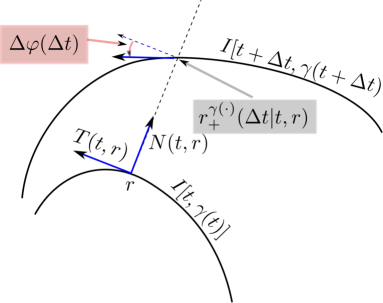
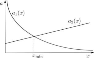
Figure 11.1: (a) Two close isolines; (b) The graphs of $a_{i}(x)$.

To discuss this control law, the following notations and quantities characterizing the moving field $D(\cdot)$ are needed:

• $\left\langle\cdot;\cdot\right\rangle$ – the standard inner product in the plane;

• $\Phi_{\beta}=\left(\begin{smallmatrix}\cos\beta&-\sin\beta\\ \sin\beta&\cos\beta\end{smallmatrix}\right)$ – the matrix of counter-clockwise rotation through angle $\beta$;

• $\nabla=\left(\begin{smallmatrix}\frac{\partial}{\partial x}\\ \frac{\partial}{\partial y}\end{smallmatrix}\right)$ – the spatial gradient;

• $D^{\prime\prime}$ – the spatial Hessian, i.e., the matrix of the second derivatives with respect to $x$ and $y$;

• $I(t,\gamma):=\{\boldsymbol{r}:D(t,\boldsymbol{r})=\gamma\}$ – the spatial isoline, i.e., the level curve of $D(t,\cdot)$ with the field level $\gamma$;

• $[T,N]=[T(t,\boldsymbol{r}),N(t,\boldsymbol{r})]$ – the Frenet frame of the spatial isoline $I[t,\gamma]$ with $\gamma:=D(t,\boldsymbol{r})$ at the point $\boldsymbol{r}$, i.e., $N(t,\boldsymbol{r})=\frac{\nabla D(t,\boldsymbol{r})}{\|\nabla D(t,\boldsymbol{r})\|}$ and the unit tangent vector $T(t,\boldsymbol{r})$ is oriented so that when traveling on $I[t,\gamma]$ one has the domain of grater values $G_{t}^{\gamma}:=\{\boldsymbol{r}^{\prime}:D(t,\boldsymbol{r}^{\prime})>\gamma\}$ to the left;

• $\varkappa$ – the signed curvature of the spatial isoline;

• $\boldsymbol{r}_{+}^{\gamma(\cdot)}(\Delta t|t,\boldsymbol{r})$ – the nearest (to $\boldsymbol{r}$) point of intersection between the ordinate axis of the Frenet frame and the displaced isoline $I[t+\Delta t,\gamma(t+\Delta t)]$, where the smooth function $\gamma(\cdot)$ is such that $\gamma(t)=D(t,\boldsymbol{r})$; see Fig. 11.1(a);

• $p^{\gamma(\cdot)}(\Delta t|t,\boldsymbol{r})$ – the ordinate of $\boldsymbol{r}_{+}^{\gamma(\cdot)}(\Delta t|t,\boldsymbol{r})$;

• $\lambda^{\gamma(\cdot)}(t,\boldsymbol{r})$ – the front velocity of the spatial isoline: $\lambda^{\gamma(\cdot)}(t,\boldsymbol{r}):=\lim_{\Delta t\to 0}$ $\frac{p^{\gamma(\cdot)}(\Delta t|t,\boldsymbol{r})}{\Delta t};$ if $\gamma(\cdot)\equiv\text{const}$ ($=D(t,\boldsymbol{r})$), the upper index ^γ(⋅) is dropped in the last three notations;

• $\alpha(t,\boldsymbol{r})$ – the front acceleration of the spatial isoline $I[t,\gamma],\gamma:=D(t,\boldsymbol{r})$:

  $$\alpha(t,r):=\lim_{\Delta t\to 0}\frac{\lambda[t+\Delta t,\boldsymbol{r}_{+}(\Delta t)]-\lambda[t,\boldsymbol{r}]}{\Delta t},\qquad\boldsymbol{r}_{+}(\Delta t):=\boldsymbol{r}_{+}(\Delta t|t,\boldsymbol{r});$$ (11.3)

• $\Delta\varphi(\Delta t|t,\boldsymbol{r})$ – the angular displacement of $T[t+\Delta t,\boldsymbol{r}_{+}(\Delta t)]$ with respect to $T[t,\boldsymbol{r}]$; see Fig. 11.1(a);

• $\omega(t,\boldsymbol{r})$ – the angular velocity of rotation of the spatial isoline $I[t,\gamma],\gamma:=D(t,\boldsymbol{r})$, i.e., $\omega(t,\boldsymbol{r}):=\lim_{\Delta t\to 0}\frac{\Delta\varphi(\Delta t|t,\boldsymbol{r})}{\Delta t}$;

• $\rho(t,\boldsymbol{r})$ – the density of isolines at time $t$ at point $\boldsymbol{r}$: $\rho(t,\boldsymbol{r}):=\lim_{\Delta\gamma\to 0}\frac{\Delta\gamma}{q(\Delta\gamma|t,\boldsymbol{r})},$ where $q(\Delta\gamma|t,\boldsymbol{r})$ is the ordinate of the nearest (to $\boldsymbol{r}$) point of intersection between the ordinate axis of the Frenet frame $[T(t,\boldsymbol{r}),N(t,\boldsymbol{r})]$ and the close isoline $I(t|t,\gamma+\Delta\gamma),\gamma:=D(t,\boldsymbol{r})$;

• $v_{\rho}(t,\boldsymbol{r})$ – the evolutional (proportional) growth rate of the above density at time $t$ at point $\boldsymbol{r}$:

  $$v_{\rho}(t,\boldsymbol{r}):=\frac{1}{\rho(t,\boldsymbol{r})}\lim_{\Delta t\to 0}\frac{\rho[t+\Delta t,\boldsymbol{r}_{+}(\Delta t)]-\rho(t,\boldsymbol{r})}{\Delta t};$$ (11.4)

• $\tau_{\rho}(t,\boldsymbol{r})$ – the tangential (proportional) growth rate of the isolines density at time $t$ at point $\boldsymbol{r}$:

  $$\tau_{\rho}(t,r):=\frac{1}{\rho(t,\boldsymbol{r})}\lim_{\Delta s\to 0}\frac{\rho(t,r+T\Delta s)-\rho(t,r)}{\Delta s};$$ (11.5)

• $n_{\rho}(t,\boldsymbol{r})$ – the normal (proportional) growth rate of the isolines density at time $t$ at point $\boldsymbol{r}$:

  $$n_{\rho}(t,r):=\frac{1}{\rho(t,\boldsymbol{r})}\lim_{\Delta s\to 0}\frac{\rho(t,r+N\Delta s)-\rho(t,r)}{\Delta s}.$$ (11.6)

• $\omega_{\nabla}(t,\boldsymbol{r})$ – the angular velocity of the gradient $\nabla D$ rotation at time $t$ at point $\boldsymbol{r}$.

11.3 Main Assumptions

Local extrema are allowed but only in a ”vicinity” $Z_{\text{near}}$ of the maximizer and at the outskirts $Z_{\text{far}}$, where the field is not assumed even smooth. In the intermediary $Z_{\text{reg}}$, the field is smooth and has no critical points and thus local extrema. To make the problem tractable, $Z_{\text{near}}$ is assumed to lie within the desired vicinity $V_{\star}$ of the maximizer, whereas the initial location is in $Z_{\text{reg}}\cup Z_{\text{near}}$. The controller should keep the robot in $Z_{\text{reg}}$ until reaching $V_{\star}$, thus avoiding detrimental effects of local extrema. To reduce the amount of technicalities, it is also assumed that the zones $Z_{\text{near}},Z_{\text{far}}$, $Z_{\text{reg}}$, and $V_{\star}$ are separated by isolines. This requirement can usually be met by properly reducing $Z_{\text{reg}}$ and $V_{\star}$, if necessary. To encompass theoretical distributions like $D(\boldsymbol{r})=c/\|\boldsymbol{r}-\boldsymbol{r}^{0}(t)\|$ or $D(\boldsymbol{r})=-c\ln\|\boldsymbol{r}-\boldsymbol{r}^{0}(t)\|$ and their sums, the field is allowed to be undefined at finitely many moving exceptional points. This is addressed in the following:

Assumption 11.3.1

There exist smooth $\gamma_{-}(t)<\gamma_{\star}(t)<\gamma_{+}(t)\in\mathbb{R}$ and continuous functions $\boldsymbol{r}_{1}(t),\ldots,\boldsymbol{r}_{k}(t)\in\mathbb{R}^{2}$ of time $t$ such that the following statements hold:

1. On $Z_{\text{reg}}:=\{(t,\boldsymbol{r}):\gamma_{-}(t)\leq D(t,\boldsymbol{r})\leq\gamma_{+}(t)\}$, the distribution $D(\cdot)$ is identical to a $C^{2}$-smooth function defined on a larger and open set, and $\nabla D(t,\boldsymbol{r})\neq 0$;

2. At any time $t$, the spatial isoline $I[t,\gamma_{-}(t)]$ is a Jordan curve that encircles $I[t,\gamma_{+}(t)]$;

3. At any time $t$, the points $\boldsymbol{r}_{1}(t),\ldots,\boldsymbol{r}_{k}(t)$ lie inside $I[t,\gamma_{+}(t)]$;

4. In the domain $Z_{\text{near}}:=\{(t,\boldsymbol{r}):\boldsymbol{r}\,\text{is inside}\,I[t,\gamma_{+}(t)]\,\text{and}\,\boldsymbol{r}\neq\boldsymbol{r}_{j}(t)\;\forall j\}$, the field $D(\cdot)$ takes values greater than $\gamma_{+}(t)$, converges to a finite or infinite limit $L_{j}(t)$ as $\boldsymbol{r}\to\boldsymbol{r}_{j}(t)$ for any $t$ and $j$, and is continuous in both $Z_{\text{near}}$ and its outer boundary $\{(t,\boldsymbol{r}):\boldsymbol{r}\in I[t,\gamma_{+}(t)]\}$;

5. In the domain $Z_{\text{far}}:=\{(t,\boldsymbol{r}):\boldsymbol{r}\,\text{is outside}\,I[t,\gamma_{-}(t)]\}$, the field $D(\cdot)$ is everywhere defined, takes values lesser than $\gamma_{-}(t)$, and is continuous in both $Z_{\text{far}}$ and its boundary $\{(t,\boldsymbol{r}):\boldsymbol{r}\in I[t,\gamma_{-}(t)]\}$;

6. The desired vicinity of the maximizer has the form $V_{\star}(t)=\{\boldsymbol{r}:D[t,\boldsymbol{r}(t)]\geq\gamma_{\star}(t)\}$;

7. For $t=0$, the initial location $\boldsymbol{r}_{\text{\rm in}}$ lies in the domain of $D(\cdot)$ and inside $I[0,\gamma_{-}(0)]$ (i.e., $D[0,\boldsymbol{r}_{\text{\rm in}}]>\gamma_{-}(0)$).

The next assumption is typically fulfilled in real world, where physical quantities take bounded values:

Assumption 11.3.2

There exists constants $b_{\omega}^{\nabla}$, $b_{\aleph}$ for $\aleph=\rho,\lambda,\omega,\varkappa,v,\alpha,n,\tau$ and $\gamma^{0}_{+},\overline{\gamma}$ such that

$$\begin{array}[]{l}|\rho|\leq b_{\rho},\;|\lambda|\leq b_{\lambda},\;|\omega|\leq b_{\omega},\;|\omega_{\nabla}|\leq b_{\omega}^{\nabla},\\ |\varkappa|\leq b_{\varkappa},\;|v_{\rho}|\leq b_{v},\;|\alpha|\leq b_{\alpha},\;|\tau_{\rho}|\leq b_{\tau},\;|n_{\rho}|\leq b_{n}\end{array}\;\forall(t,\boldsymbol{r})\in Z_{\text{reg}};\\ \gamma_{+}(t)\leq\gamma^{0}_{+},|\dot{\gamma}_{i}(t)|\leq\overline{\gamma}\quad\forall t,i=\pm,\star.$$ (11.7)

The only assumption about the robot capacity with respect to the field is that the mobility of the former exceeds that of the latter: in the main operational zone $Z_{\text{reg}}$, the maximal speed of the robot is greater than the front speed of the concerned isoline of the field: $v>|\lambda(t,\boldsymbol{r})|$. Moreover, if the level $\gamma_{-}(\cdot)$ or $\gamma_{\star}(\cdot)$ is not constant, the robot is capable to remain inside the moving isoline $I[t,\gamma_{-}(t)]$ and inside $I[t,\gamma_{\star}(t)]$.

All afore-mentioned strict inequalities are protected from degradation as time progresses. To quanify this the notation $f\ntriangleright g$ in $Z$ is used to express that $\exists\varepsilon>0:f(t,\boldsymbol{r})\geq g(t,\boldsymbol{r})+\varepsilon\;\forall(t,\boldsymbol{r})\in Z$; the relation $\ntriangleleft$ is defined likewise.

Assumption 11.3.3

The following inequalities hold:

$$\rho(t,\boldsymbol{r})\ntriangleright 0,\quad v\ntriangleright|\lambda(t,\boldsymbol{r})|+\rho^{-1}\overline{\gamma},\;\quad\text{\rm in}\;Z_{\text{reg}};\qquad\gamma_{-}(t)\ntriangleleft\gamma_{\star}(t)\ntriangleleft\gamma_{+}(t)\quad\text{\rm in}\;[0,\infty).$$ (11.8)

11.4 Summary of Main Results

The first theorem shows that the control objective can always be achieved by means of the control law Eq.(11.2):

Theorem 11.4.1

Suppose that Assumptions 11.3.1–11.3.3 hold. Then there exist parameters $v_{\ast},\mu,\theta_{0}$ of the controller Eq.(11.2) such that the following claim holds:

1. The controller Eq.(11.2) brings the robot to the desired vicinity of a maximizer in a finite time $t_{0}$ and keeps it there afterwards: $\boldsymbol{r}(t)\in V_{\star}(t)$ for $t\geq t_{0}$.

Moreover, for any compact domain $D\subset\mathbf{int}\{\boldsymbol{r}:(0,\boldsymbol{r})\in Z_{\text{reg}}\}$, there exist common values of the parameters for which (i) holds whenever the initial location $\boldsymbol{r}_{\text{\rm in}}\in D$.

The remainder of the section is devoted to discussion of controller parameters tuning. The parameters $\theta_{0},v_{\ast}$ in Eq.(11.2) are chosen prior to $\mu$. Whereas $\theta_{0}$ is arbitrary, $v_{\ast}$ is chosen so that:

$$v\ntriangleright|\lambda|+\rho^{-1}v_{\ast}\quad\text{in}\quad Z_{\text{reg}},\qquad v_{\ast}>\overline{\gamma},$$ (11.9)

This is possible thanks to Eq.(11.8). The choice of $\mu$ is prefaced by picking constants $\Delta_{\nabla}>0$ and $\Delta_{\gamma}>0$ such that

$$\rho(t,\boldsymbol{r})\geq\Delta_{\nabla}\quad\forall(t,\boldsymbol{r})\in Z_{\text{reg}},\quad\gamma_{-}(t)+\Delta_{\gamma}\leq\gamma_{\star}(t)\leq\gamma_{+}(t)-\Delta_{\gamma},\\ D[0,\boldsymbol{r}_{\text{\rm in}}]\geq\gamma_{-}(0)+\Delta_{\gamma}/2,$$ (11.10)

This is possible by the same argument. The parameter $\mu$ is chosen so that for some $k=1,2,\ldots$,

$$\mu(v_{\ast}-\overline{\gamma})\ntriangleright-2\omega-\varkappa v_{T}+2\frac{\tau_{\rho}\overline{\gamma}}{\rho}+2\frac{v_{\rho}\overline{\gamma}}{v_{T}\rho}-\frac{\alpha}{v_{T}}+\frac{n_{\rho}\overline{\gamma}^{2}}{v_{T}\rho^{2}},$$ (11.11a)

$$\text{where}\;v_{T}:=\pm\sqrt{v^{2}-\left[\lambda+\rho^{-1}\overline{\gamma}\right]^{2}},\quad\text{in}\quad Z_{\text{reg}};$$

$$\mu\ntriangleright\frac{\omega+\tau_{\rho}(\lambda-v)}{\rho(v-\lambda)-v_{\ast}}\quad\text{in}\quad Z_{\text{reg}};$$ (11.11b)

$$\mu(v_{\ast}-\overline{\gamma})>\left\{\begin{array}[]{l}a_{1}(k):=2b^{\nabla}_{\omega}\left[1+\frac{1}{k}\right]+2v\sqrt{b_{\varkappa}^{2}+b_{\tau}^{2}}\left[2+\frac{1}{k}\right],\\ a_{2}(k):=2b_{\rho}\frac{(2k+1)v+2\pi(k+1)\left(b_{\lambda}+\Delta_{\nabla}^{-1}\overline{\gamma}\right)}{\Delta_{\gamma}}\end{array}\right..$$ (11.11e)

The following theorem ensures the correct behaviour is exhibited by the robot:

Theorem 11.4.2

Suppose that Assumptions 11.3.1–11.3.3 hold and the controller parameters satisfy Eq.(11.9) and Eq.(11.11a)–Eq.(11.11e). Then (i) from Theorem 11.4.1 is true.

11.5 Simulations

Simulations were carried out with the point-wise robot Eq.(11.1) driven by the control law Eq.(11.2). The numerical values of the parameters used for simulations are shown in Table 11.1 (where $u_{d}$ is the unit of measurement of $d=D(t,\boldsymbol{r})$ and the controller parameters were chosen according to recommendations from Theorem 11.4.2). The control was updated with a sampling time of $0.1s$.

$v$	$1m/s$
$v_{*}$	$0.299u_{d}/s$

$\mu$	$0.8rad/u_{d}$
$\theta_{0}$	$1.5rad$

Table 11.1: Simulation parameters for extremum-seeking controller.

Fig. 11.2 displays the results of tests in a linear field with the orientation angle of $0.5$ rad and the ascension rate of $0.3m^{-1}$; the grey intensity is proportional to the field value. The steady state angular error may be computed to be $\approx 0.082rad$. Fig. 11.2 shows that the heading converges to approximately $0.582rad$, thus displaying a good match.

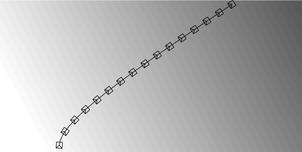
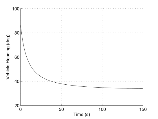
Figure 11.2: Behavior in a linear field; (a) Path; (b) Robot’s orientation.

Fig. 11.3 presents the results of tests in an unsteady field with a moving source. The source $\boldsymbol{r}^{0}(t)$ moves to the right at the speed of $0.3ms^{-1}$, $D(t,\boldsymbol{r})$ is a radial field corrupted by two plain waves and is given by:

$$D(t,\boldsymbol{r})=-0.8\cdot\lVert\boldsymbol{r}-\boldsymbol{r}^{0}(t)\rVert+5\cdot\left[\sin(0.05\cdot x)+\sin(0.05\cdot y)\right].$$

As can be seen, the robot converges to the source (whose path is depicted by the solid black line) and then wheels around it in a close proximity, thus displaying its current location and highlighting its displacement. ‘Wheeling’ commences when the robot achieves the desired vicinity of the source and is unavoidable since the robot’s speed exceeds that of the source.

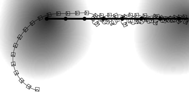
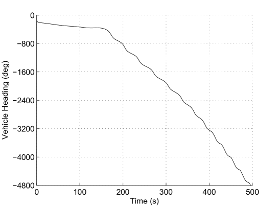
Figure 11.3: Seeking a moving source; (a) Path; (b) Robot’s orientation.

In Fig. 11.4, the same simulation setup was used, except measurement noise and kinematic constraints were added. The robot’s heading was not allowed to change faster than $0.5rads^{-1}$, which in fact transforms Eq.(11.1) into the non-holonomic Dubins-car model since the robot’s speed is constant by Eq.(11.2). The field readings were corrupted by a random additive noise uniformly distributed over the interval $[-2.5,2.5]$. It may be seen that nearly the same behavior is observed.

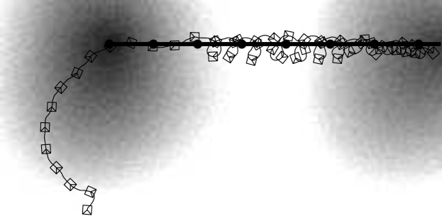
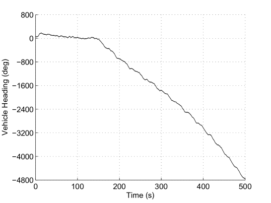
Figure 11.4: Seeking a moving source under measurement noise and kinematic constraints; (a) Path; (b) Robot’s orientation.

In Fig. 11.5, the plain waves were enhanced to produce a large number of local maxima and the source was stopped: the updated field distribution is given by:

$$D(t,\boldsymbol{r})=-0.8\cdot\lVert\boldsymbol{r}-\boldsymbol{r}^{0}\rVert+10\cdot\left[\sin(1.0\cdot x)+\sin(1.0\cdot y)\right].$$

Fig. 11.5 shows that despite the local maxima, the vehicle stills converges to the source of the distribution. This is in a sharp contrast to the pure gradient ascent method for which every local maximum constitutes a trap. A presumable reason for this property of the proposed algorithm is that it needs special tuning to be trapped by a small enough vicinity of a maximizer. Whenever it is tuned for a specific vicinity ”size”, it demonstrates the capability to go through and escape from smaller traps. A detailed analysis of this interesting and promising property is a subject of future research.

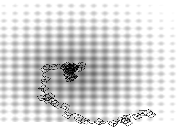
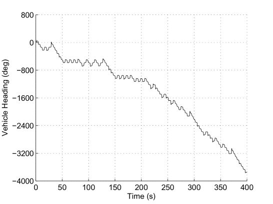
Figure 11.5: Seeking a source in the presence of multiple local maxima; (a) Path; (b) Robot’s orientation.

Simulations were also carried out for a realistic model of a time varying field caused by a constant-rate emanation of a certain substance (such as heat or gas) from a moving point-wise source and its subsequent diffusion in an isotropic two-dimensional medium. In many cases, this process is described by the heat equation $\partial D/\partial t=\rho\Delta D+\delta[\boldsymbol{r}-\boldsymbol{r}^{0}(t)]$. Here $\Delta$ is the spatial Laplacian, $\rho=16000m^{2}s^{-1}$ is the diffusion rate, $\delta$ is the spatial Dirac delta-function, $\boldsymbol{r}^{0}(t)$ is the source location, and the emanation rate was set to unity. The field distribution was calculated prior to navigation tests by the finite difference method. In doing so, the time and space steps were $0.001s$ and $4m$, respectively; the results were stored with the sampling rate $1s$. During the navigation test, the distribution value was obtained through trilinear interpolation over spatial and temporal variables. To initialize the distribution, the source stayed still for the first $100s$ and only then commenced motion. The vehicle turning rate was bounded by $0.5rads^{-1}$. The results of these simulations are shown in Fig. 11.6. It may be seen that the robot solves the source seeking task.

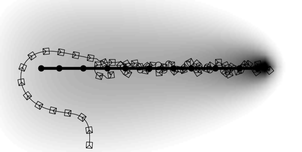
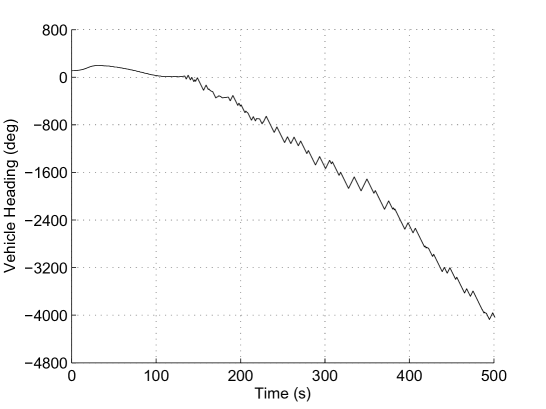
Figure 11.6: Seeking a moving diffusion source; (a) Path; (b) Robot’s orientation.

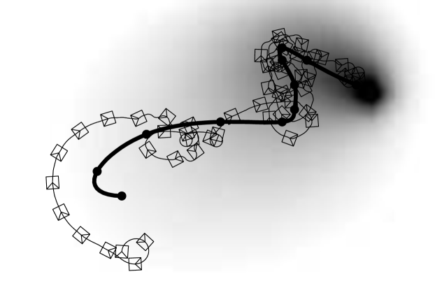
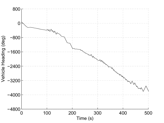
Figure 11.7: Seeking an irregularly moving diffusion source; (a) Path; (b) Robot’s orientation.

11.6 Experiments

Experiments were carried out with an Activ-Media Pioneer 3-DX differential drive wheeled robot using its on-board PC and the Advanced Robot Interface for Applications (ARIA 2.7.2), which is a C++ library providing an interface to the robot s angular and translational velocity set-points.

The origin of the reference frame was co-located with the center of the robot in its initial position, its ordinate axis is directed towards the viewer in Figs. 11.8, 11.11, and 11.14. Three scenarios were tested:

• A steady virtual point-wise source was located at the point with coordinates $(0,3.5)m$ in Fig. 11.8. The experiment was run for $175s$.

• A virtual point-wise source moved from the point with the coordinates $(0,3.5)m$ with a constant translational velocity $(0,-0.02)ms^{-1}$ outwards the viewer in Fig. 11.11. The experiment was run for $175s$ so that the final position of the source coincided with the origin of the reference frame.

• A virtual point-wise source moved at the constant speed $0.02ms^{-1}$ from the same point along the piece-wise linear path through the points $(0,3.5)m$, $(0.6,2.5)m$, $(-0.6,1.0)m$ and $(0,0)m$ in Fig. 11.14. The experiment was run for $213s$.

The path of the source is displayed in Fig. 11.11 by a long black tape, and in Fig. 11.14 by a long gray tape. The examined field was minis the distance to the source, which was accessed via odometry, whereas the source motion was virtual and emulated by computer. The orientation of the robot $\theta_{act}(t)$ was also captured via odometry.

The parameters used in the experiments are shown in Table 11.2.

$v$	$0.15m/s$
$v_{\ast}$	$0.12u_{d}/s$

$\mu$	$4.0rad/u_{d}$
$\theta_{0}$	$0rad$

Table 11.2: Experimental parameters for extremum-seeking controller.

The control law was updated at the rate of $0.1s$. The control law Eq.(11.2) was used as a generator of the velocity reference signal. Tracking of the generated velocity profile was accomplished by means of simple PD controllers.

Typical experimental results are presented on Figs. 11.8–11.16. In these experiments, like in the others, the robot successfully reached the source and then tracked it until the end of the experiment. In Figs. 11.9, 11.12, and 11.15, the final maximum steady state distance to the source is upper bounded by $0.5m$. This approximately equals the radius of the desired margin $R_{\star}$ employed in computation of the controller parameters, which was chosen with regard to the turning capacity of the robot at the selected speed.

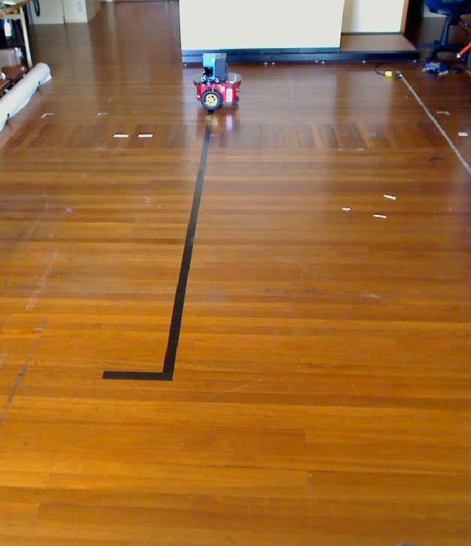
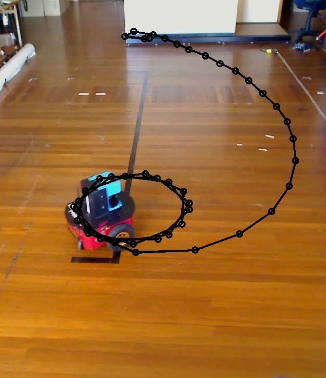
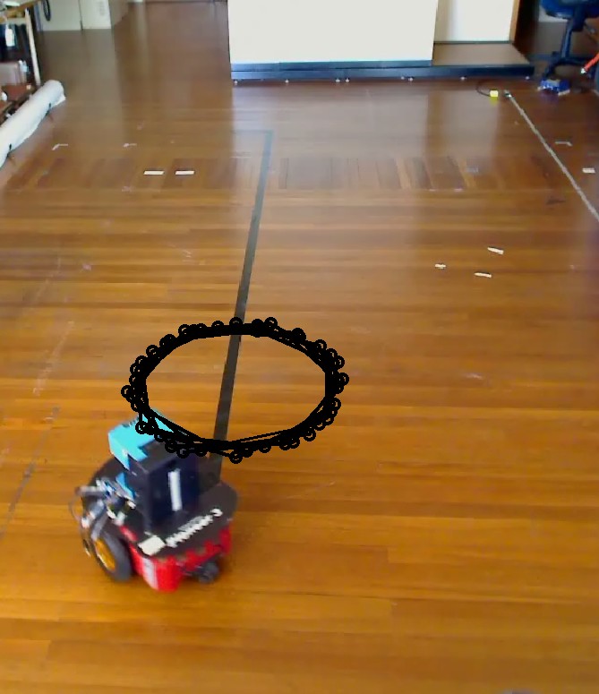
Figure 11.8: Sequence of images showing the experiment.

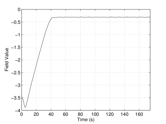
Figure 11.9: Evolution of the field value over the experiment. Field value is in metres.

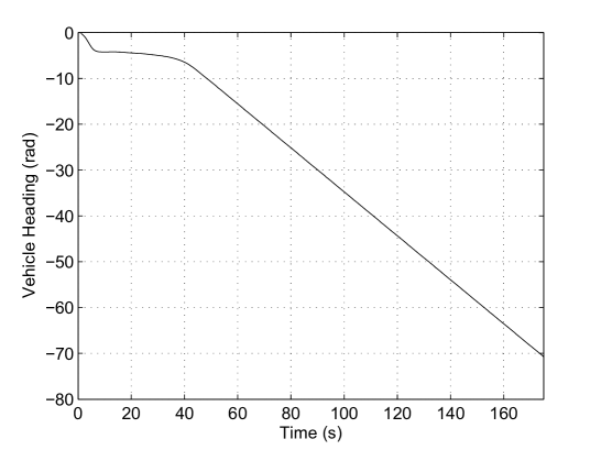
Figure 11.10: Evolution of the vehicle orientation over the experiment.

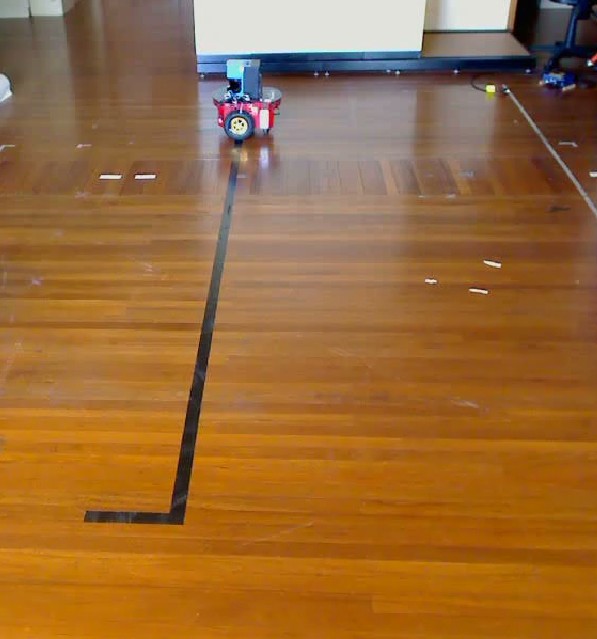
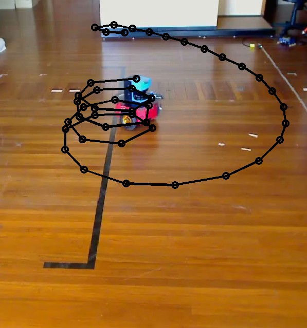
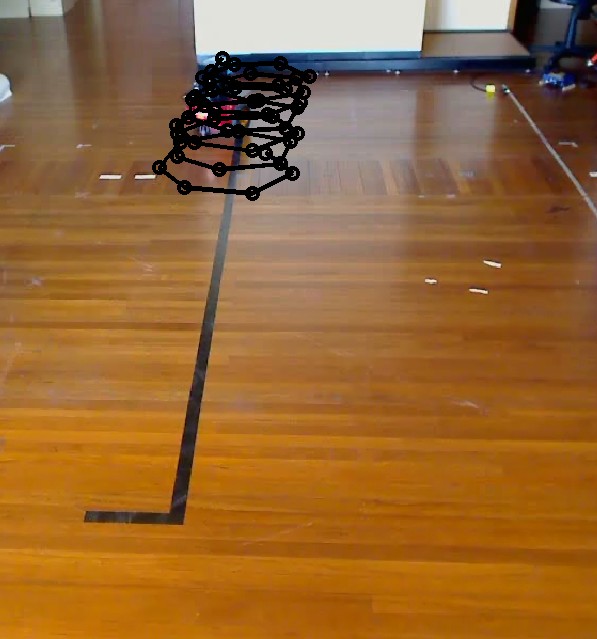
Figure 11.11: Sequence of images showing the experiment (moving field).

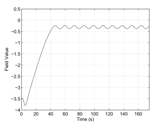
Figure 11.12: Evolution of the field value over the experiment. Field value is in metres.

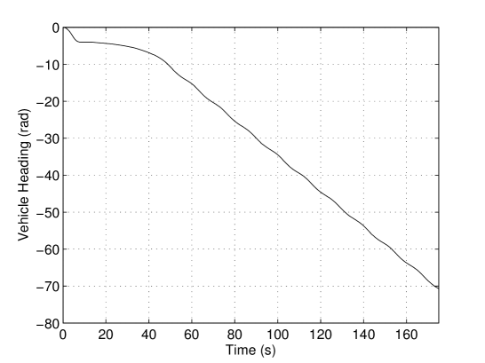
Figure 11.13: Evolution of the vehicle orientation over the experiment.

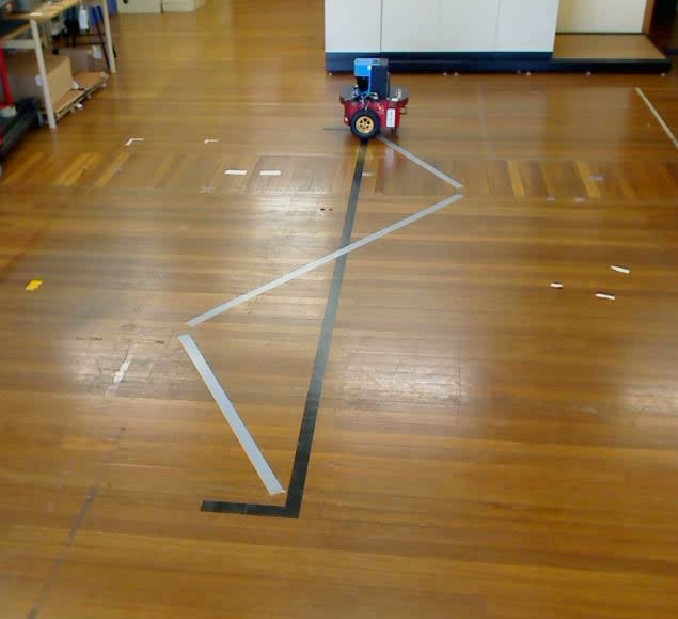
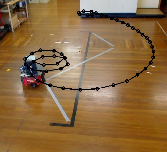
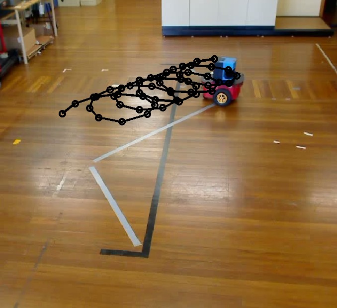
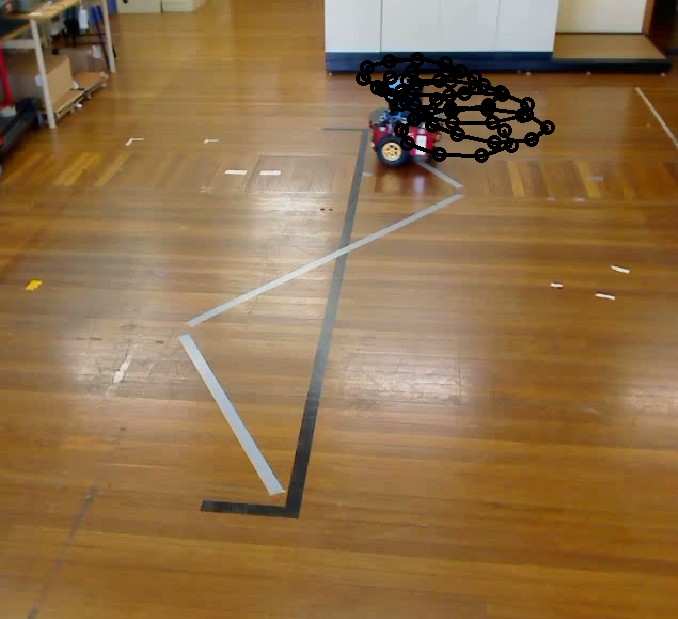
Figure 11.14: Sequence of images showing the experiment (irregularly moving field).

Figure 11.15: Evolution of the field value over the experiment. Field value is in metres.

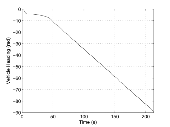
Figure 11.16: Evolution of the vehicle orientation over the experiment.

11.7 Summary

A single kinematically controlled mobile robot traveling in a planar region supporting an unknown and unsteady field distribution is considered, where only the current value of the field is known to the robot. A reactive navigation strategy is presented that drives the robot towards the time-varying location where the field distribution attains its spatial maximum and then keeps the robot in the pre-specified vicinity of that point. The applicability and performance of the proposed guidance approach are confirmed by extensive simulation tests and experiments with a real wheeled robot.

Chapter 12 Tracking the Level Set of a Scalar Field

This chapter introduces a method for tracking a specified level set or isoline of an environmental scalar field. To achieve this, a sliding mode control law is designed which can provably achieve the desired behaviour, given set of assumptions about the field. Simulations and experimental results are given to confirm the viability of the proposed method.

12.1 Introduction

Recent environmental disasters have highlighted the need for effective tools capable of timely detection, exploration, and monitoring of environmental boundaries. Some of these distributed phenomena can be observed as a whole using large scale sensors. However, there are many scenarios where such observation is troublesome, the quantity can only be realistically measured using local sensors in a point-wise fashion at a particular location (see e.g. [49, 128, 195]). Observation by means of a distributed network of static sensors typically requires high deployment density and considerable computational and communication loads to provide good accuracy [197, 252]. More effective use of sensors is achieved in mobile networks, where each sensor explores many locations. This is especially beneficial whenever the interest is focused not so much on the entire distributed phenomenon as on some dependent structure of a lower dimension, like the boundary of an oil spill or radioactively contaminated area. To derive this benefit, the mobile sensor should be equipped with a motion control system by which it can detect and track this structure.

Recently, such problems have gained much interest in control community. Among their basic setups, there is tracking of environmental level sets: the robot should reach and then track the curve where an unknown scalar field assumes a specific value and which is thus the boundary of the area with greater values. In doing so, the control law should use only point-wise field measurements along the robot path.

Many works in this area assume access to the field gradient or even higher derivatives data such as the curvature of the isoline (see e.g. [213, 317, 361, 138]). Some examples include gradient-based contour estimation by mobile sensor networks [213, 31, 317], centralized control laws originating from the ‘snake’ algorithms in image segmentation [213, 31], cooperative distribution of the sensors over the estimated contour with minimal latency [317], artificial potential approach based on direct access to the gradient [138], collaborative estimation of the gradient and Hessian of the noise-corrupted field as the basis for driving the center of a rigid formation of multiple sensors along a level curve [361]. However derivative-dependent data is often unavailable, whereas its estimation requires access to the field values at several nearby locations. Even in the multiple sensor scenario, such access may be degraded by limitations on communication and may require ineffective concentration of sensors into a compact cluster.

A single mobile sensor with access to only point field values is the main target for gradient-free approaches (see e.g. [20, 154, 49, 13]). Control via switches between two steering angles depending on whether the current field value is above or below the threshold have been proposed [364, 145]. Similar approach with a larger set of alternatives has been applied to an underwater vehicle equipped with a profile sonar [20]. These methods typically result in a zigzagging behavior and rely in effect on systematic side exploration maneuvers to collect rich enough data. A method to control an unmanned aerial vehicle has been proposed based on segmentation of the infrared local images of a forest fire [50]. These works are based, more or less, on heuristics and provide no rigorous and completed justification of the proposed control laws. A linear PD controller fed by the current field value has been proposed for steering a unicycle-like vehicle along a level curve of a field given by a radial harmonic function, and a local convergence result was established for a vehicle with unlimited control range [21]. A sliding mode control method for tracking environmental level sets without gradient estimation was offered in [233].

The characteristic feature of the previous research is that it dealt with only steady fields, which means that the reference level curve does not move or deform. However in real world, environmental fields are almost never steady and often cannot be well approximated by steady fields, whereas the theory of tracking the level sets for dynamic fields lies in uncharted territory. As a particular case, this topic includes navigation and guidance of a mobile robot towards an unknowingly maneuvering target and further escorting it with a pre-specified margin on the basis of a single measurement that decays as the sensor goes away from the target, like the strength of the infrared, acoustic, or electromagnetic signal, or minus the distance to the target. Such navigation is of interest in many areas [16, 104, 232]; it carries a potential to reduce the hardware complexity and cost and improve target pursuit reliability. The mathematically rigorous analysis of a navigation law for such problem was offered in [232] in the very special case of the unsteady field – the distance to an unknowingly moving Dubins-like target. However the results of [232] are not applicable to more general dynamic fields.

The navigation strategy considered in this chapter develops some ideas set forth in [233]; in particular, spatial gradient estimates and systematic exploration maneuvers are not employed. However in [233], only the case of static fields was examined. In this work, it is shown that those ideas remain viable for much more general scenarios with dynamic fields. Conditions necessary for a Dubins-like vehicle to be capable of tracking the moving and deforming level set of a dynamic field are established. It is shown that whenever slight and partly unavoidable enhancements of these necessary conditions hold, the problem can be solved by the proposed controller. This is done by means of a mathematically rigorous non-local convergence result, which contains recommendations on the controller parameters tuning.

All proofs of mathematical statements are omitted here; they are available in the original manuscript [219].

The body of this chapter is organized as follows. In Sec. 12.2 the problem is formally defined, in Sec. 12.3 the the main assumptions are described. The main results are outlined in Sec. 12.4. Simulations and experiments are presented in Secs. 12.5 and 12.6. Finally, brief conclusions are given in Sec. 12.7.

12.2 Problem Statement

A planar mobile robot is considered, which travels with a constant speed $v$ and is controlled by the time-varying angular velocity $u$ limited by a given constant $\overline{u}$. The robot’s workspace hosts an unknown and time-varying scalar field $D(t,\boldsymbol{r})\in\mathbb{R}$. Here $\boldsymbol{r}:=(x,y)^{\top}$ is the vector of the absolute Cartesian coordinates $x,y$ in the plane $\mathbb{R}^{2}$ and $t$ is time. The objective is to steer the robot to the level curve $D(t,\boldsymbol{r})=d_{0}$ where the distribution assumes a given value $d_{0}$ and to ensure that the robot remains on this curve afterwards, circulating along it at the given absolute speed $v$. The on-board control system has access to the distribution value $d(t):=D(t,x,y)$ at the vehicle current location $x=x(t),y=y(t)$ and is capable to access the rate $\dot{d}(t)$ at which this measurement evolves over time $t$. However, neither the partial derivative $D^{\prime}_{t}$, nor $D^{\prime}_{x}$, nor $D^{\prime}_{y}$ is accessible.

The kinematic model of the robot is as follows:

$$\begin{array}[]{l}\dot{x}=v\cos\theta,\\ \dot{y}=v\sin\theta,\end{array},\quad\dot{\theta}=u,\quad|u|\leq\overline{u},\quad\begin{array}[]{l}x(0)=x_{\text{in}}\\ y(0)=y_{\text{in}}\end{array},\quad\theta(0)=\theta_{\text{in}},$$ (12.1)

Here $\theta$ gives the robot orientation. It is required to design a controller that ensures the convergence $D[t,x(t),y(t)]\to d_{0}$ as $t\to\infty$. In this chapter, the following navigation law is examined:

$$u(t)=-\text{\bf sgn}\{\dot{d}(t)+\chi[d(t)-d_{0}]\}\bar{u},\qquad d(t)=D[t,x(t),y(t)],$$ (12.2)

Here $\chi(\cdot)$ is a linear function with saturation:

$$\chi(p):=\begin{cases}\gamma p&\text{if}\;|p|\leq\delta\\ \text{\bf sgn}(p)\mu&\text{otherwise}\end{cases},\qquad\mu:=\gamma\delta.$$ (12.3)

The gain coefficient $\gamma>0$ and the saturation threshold $\delta>0$ are design parameters.

For the discontinuous control law Eq.(12.2), the desired dynamics [339] is given by $\dot{d}(t)=-\chi[d(t)-d_{0}]$.

12.3 Main Assumptions

The notation describing the field is taken from Chapt. 11. The conditions employed in this chapter are described by the following:

Proposition 12.3.1

Suppose that the robot moves so that it remains on the required isoline $D[t,r(t)]\equiv d_{0}$ and in a vicinity of this isoline, the function $D(\cdot,\cdot)$ is twice continuously differentiable and $\nabla D(\cdot,\cdot)\neq 0$. Then at any time the front speed of the isoline at the robot location does not exceed the speed of the robot

$$\left|\lambda[t,r(t)]\right|\leq v,$$ (12.4)

the robot’s velocity

$$\vec{v}=v\vec{e},\qquad\vec{e}:=\left(\begin{array}[]{c}\cos\theta\\ \sin\theta\end{array}\right)$$ (12.5)

has the form

$$\vec{v}=\lambda N\pm T\sqrt{v^{2}-\lambda^{2}},$$ (12.6)

and the following inequality is true

$$\left|\pm 2\omega+\frac{\alpha}{\sqrt{v^{2}-\lambda^{2}}}+\varkappa\sqrt{v^{2}-\lambda^{2}}\right|\leq\overline{u}.$$ (12.7)

In $\pm$, the sign $+$ is taken if the robot travels along the isoline in the positive direction (i.e., so that the domain $\{\boldsymbol{r}:D(t,\boldsymbol{r})>d_{0}\}$ is to the left), and $-$ is taken otherwise.

For the control objective to be attainable, Eq.(12.4) and Eq.(12.7) should hold at the current location of the robot at any time. Since this location is not known in advance, it is reasonable to extend this requirement on all points on the isoline. However, some form of controllability is also required to make the objective of driving the robot to the pre-specified isoline realistic. For example, the robot should be capable of moving from a given isoline $I(t,d_{\ast})$ to the area of larger field values $\{\boldsymbol{r}:D(t,\boldsymbol{r})>d_{\ast}\}$, as well as to that of smaller ones. Since remaining on the isoline implies $\dot{d}=0$, this property means that the sign of the second derivative $\ddot{d}$ can be made both positive and negative by respective choices of feasible controls $u\in[-\overline{u},\overline{u}]$.

It is assumed that such controllability holds in the entire zone of the robot’s maneuver $\mathcal{M}$, which is characterized by the extreme values $d_{-}\leq d_{+}$ taken by the field in this zone:

$$\mathcal{M}:=\{(t,\boldsymbol{r}):d_{-}\leq D(t,\boldsymbol{r})\leq d_{+}\}$$ (12.8)

It is also assumed this contains the required isoline $d_{-}\leq d_{0}\leq d_{+}$. Finally, it is assumed that the above strict inequalities do not degrade as time progresses or location $\boldsymbol{r}$ goes to infinity. As a result, the following assumption is arrived at:

Assumption 12.3.1

The field $D(\cdot,\cdot)$ is twice continuously differentiable in the domain Eq.(12.8) and there exist constants $\Delta_{\lambda}>0$ and $\Delta_{u}>0$ such that the following enhanced analogs of Eq.(12.4) and Eq.(12.7) hold:

$$\left|\lambda\right|\leq v-\Delta_{\lambda},\quad\left|\pm 2\omega+\frac{\alpha}{\sqrt{v^{2}-\lambda^{2}}}+\varkappa\sqrt{v^{2}-\lambda^{2}}\right|\leq\overline{u}-\Delta_{u}\qquad\forall(t,r)\in\mathcal{M},$$ (12.9)

where the second inequality is true with the both signs in $\pm$.

Since the trajectory of the robot is smooth, it is natural to exclude isoline singularities:

Assumption 12.3.2

The field has no spatial singularities $\nabla D\neq 0$ in the domain Eq.(12.8), and this property does not degrade as time progresses: there exists $b_{\rho}>0$ such that $\rho(t,\boldsymbol{r})=\|\nabla D(t,\boldsymbol{r})\|\geq b_{\rho}^{-1}\;\forall(t,\boldsymbol{r})\in\mathcal{M}$.

The next assumption is typically fulfilled in real world, where physical quantities take bounded values:

Assumption 12.3.3

There exist constants $b_{\lambda},b_{\tau},b_{n},b_{\varkappa},b_{v},b_{\alpha}$ such that the following inequalities hold:

$$|\lambda|\leq b_{\lambda},\quad|\tau_{\rho}|\leq b_{\tau},\quad|n_{\rho}|\leq b_{n},\quad|\varkappa|\leq b_{\varkappa},\quad|v_{\rho}|\leq b_{v},\quad|\alpha|\leq b_{\alpha}\qquad\forall(t,r)\in\mathcal{M}.$$ (12.10)

The last assumption is partly underlaid by the fact that under the control law Eq.(12.2) with properly tuned parameters, the vehicle initially moves with $u\equiv\pm\overline{u}$ over an initial circle $C_{\pm}^{\text{in}}$, which is defined as the related path starting with the given initial data from Eq.(12.1). It is required that these circles lie in the operational zone Eq.(12.8), along with the encircled disc’s $D_{\pm}^{\text{in}}$ (also called initial). Furthermore, there exists some initial time interval during which the average angular speed of the spatial gradient rotation is less than the maximal turning rate of the robot. This leads to the following:

Assumption 12.3.4

There exists a natural $k$ such that during the time interval $\left[0,T_{k}\right],$ $T_{k}$ $:=$ $\frac{2\pi k}{\overline{u}}$, (a) the gradient $\nabla D(t,\boldsymbol{r}_{\text{in}}),\boldsymbol{r}_{\text{in}}:=(x_{\text{in}},y_{\text{in}})^{\top}$ rotates through an angle that does not exceed $2\pi(k-1)$ and (b) the both initial disc’s lie in the domain Eq.(12.8), i.e., $[0,T_{k}]\times D_{\pm}\subset\mathcal{M}$.

12.4 Summary of Main Results

The main theoretical result may now be stated:

Theorem 12.4.1

Suppose that Assumptions 12.3.1–12.3.4 hold and the parameters $\gamma,\mu=\gamma\delta$ of the controller Eq.(12.2) satisfy the following inequalities, where $\mu_{\ast}$ $:=$ $b_{\rho}\mu$ and $\sigma(\mu_{\ast})$ $:=$ $\sqrt{\Delta_{\lambda}^{2}-2v\mu_{\ast}-\mu^{2}_{\ast}}$:

$$0<\mu_{\ast}<\sqrt{v^{2}+\Delta_{\lambda}^{2}}-v,\quad\left(3b_{\tau}+\frac{b_{\varkappa}+2b_{v}+\gamma+b_{n}\mu_{\ast}}{\sigma(\mu_{\ast})}+\frac{b_{\alpha}}{\sigma(\mu_{\ast})^{3}}\right)\mu_{\ast}<\Delta_{u}.$$ (12.11)

Then the robot driven by the navigation law Eq.(12.2) achieves the control objective $d(t)\xrightarrow{t\to\infty}d_{0}$ and moves in the domain Eq.(12.8).

12.5 Simulations

Simulations were carried out with the Dubins-like robot Eq.(12.1) driven by the control law Eq.(12.2). The numerical values of the parameters used for simulations are shown in Table 12.1, where $u_{d}$ is the unit of measurement of $d=D(t,\boldsymbol{r})$ and the controller parameters were chosen based on recommendations from Theorem 12.4.1. The control was updated with the sampling time of $0.1s$.

$v$	$1m/sec$
$\mu$	$0.5u_{d}/sec$
$\gamma$	$0.04sec^{-1}$

Table 12.1: Simulation parameters for level set tracking controller.

Figs. 12.1 and 12.1 present the results of tests in the moving radial field

$$D(t,\boldsymbol{r})=70-0.8\cdot\lVert\boldsymbol{r}-\boldsymbol{r}^{0}(t)\rVert,$$

where the source $\boldsymbol{r}^{0}(t)$ moves to the right at the speed of $0.3m/sec$. Fig. 12.1 demonstrates successful convergence to the desired field value $d_{0}=30$. Fig. 12.1 shows the related path of the robot; in Figs. 12.1, 12.2 and 12.3, the position of the field source is depicted by the solid black line. Since the isoline of the unsteady radial field at hand is a circle undergoing a constant velocity displacement, the robot that moves with a constant speed and does not leave this isoline should trace a cycloid (either curtate or prolate). As can be seen in Fig. 12.1, it does trace a prolate cycloid-like path, up to the transient.

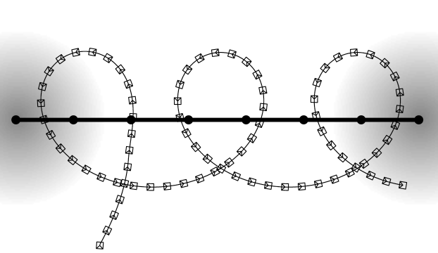
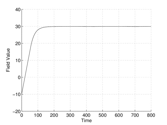
Figure 12.1: Simulations with an unsteady radial field; (a) Path; (b) Robot’s orientation. Time is in seconds, field value is in arbitrary units.

In Figs. 12.2 and 12.2, the effect of the measurement noise was examined in a similar simulation setup. Specifically, the measurements $d(t)$ and $\dot{d}(t)$ were individually corrupted by random additive noises uniformly distributed over the intervals $[-2.5u_{d},2.5u_{d}]$ and $[-2.0u_{d}/sec,2.0u_{d}/sec]$, respectively. The scalar field was corrupted by sinusoidal plane waves:

$$D(t,\boldsymbol{r})=70-0.8\cdot\lVert\boldsymbol{r}-\boldsymbol{r}^{0}(t)\rVert+5\cdot\left[\sin(0.05\cdot x)+\sin(0.05\cdot y)\right].$$

Figs. 12.2 and 12.2 show that the control objective is still achieved with a good exactness, though the path becomes less regular.

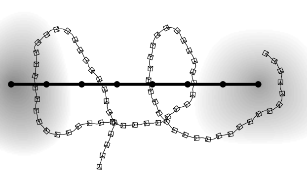
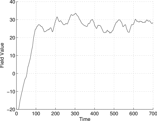
Figure 12.2: Simulations with measurement noise; (a) Path; (b) Robot’s orientation. Time is in seconds, field value is in arbitrary units.

Simulations were also carried out for a more realistic model of a time-varying field caused by a constant-rate emanation of a certain substance, which was taken to be the same as that in Chapt. 11. The results of these simulations are shown Figs. 12.3 and 12.3, where the source of diffusion undergoes irregular motion depicted by the solid black curve in Fig. 12.3. The small impulse in the field value at $\approx 600s$ is a result of breaking the limitations revealed by Proposition 12.3.1. As can be seen, the control objective is still achieved with a good accuracy.

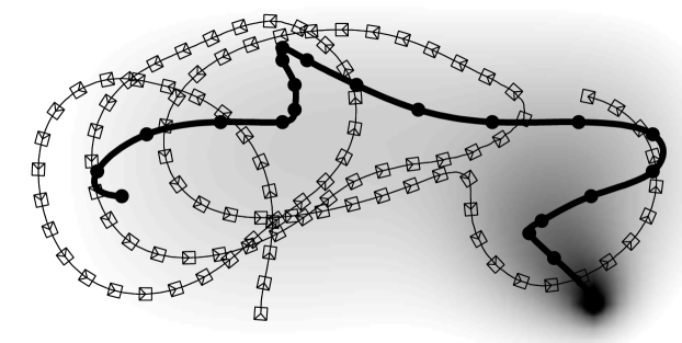
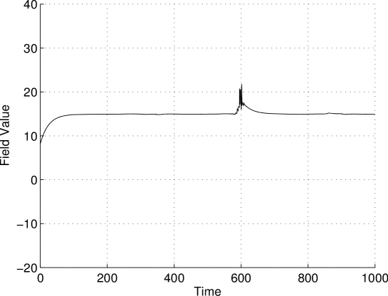
Figure 12.3: Simulations with a heat source; (a) Path; (b) Robot’s orientation. Time is in seconds, field value is in arbitrary units.

12.6 Experiments

Experiments were carried out with an Activ-Media Pioneer 3-DX wheeled robot using its on-board PC and the Advanced Robot Interface for Applications (ARIA 2.7.2), which is a C++ library providing an interface to the robot s angular and translational velocity set-points.

The origin of the reference frame was co-located with the center of the robot in its initial position, its ordinate axis is directed towards the viewer in Figs. 12.4 and Eq.(12.6). In two groups of experiments, a virtual point-wise source of the scalar field moved, respectively, as follows:

1. The source moved from the point with the coordinates $(0,3.5)m$ with a constant translational velocity $(0,-0.02)ms^{-1}$ outwards the viewer in Fig. 12.4. The experiment was run for $175s$ so that the final position of the source coincided with the origin of the reference frame.

2. The source moved at the constant speed $0.02ms^{-1}$ from the same initial position along a piece-wise linear path through the points $(0,3.5)m$, $(0.6,2.5)m$, $(-0.6,1.0)m$ and $(0,0)m$; the motion was still outwards the viewer in Fig. 12.6. The experiment was run for $213s$.

The path of the source is displayed in Fig. 12.4 by a long black tape, and in Fig. 12.6 by long gray tape. The examined field was minus the distance to the moving source, which was accessed via odometry, whereas the source motion was virtual and emulated by computer.

The parameters used in the experiments are shown in Table 12.2.

$v$	$0.15m/s$
$\gamma$	$0.2s^{-1}$

$\mu$	$0.12m/s$
$d_{0}$	$-0.8m$

Table 12.2: Experimental parameters for level set tracking controller.

In the control law Eq.(12.2), the signum function $\text{\bf sgn}(\cdot)$ was replaced by a linear function with saturation $\text{\bf sat}\,(S):=\text{\bf sgn}(S)\cdot\text{min}\{10\cdot|S|,\bar{u}\}$ with $\bar{u}=1.0$. The control law was updated at the rate of $0.1s$.

Typical results of experiments from the first and second groups are presented on Figs. 12.4, 12.5 and 12.6, 12.7, respectively. The desired field value is indicated by the thick black line in Figs. 12.5 and 12.7. In these experiments, like in the others, the robot successfully arrives at the desired field value and then maintains it until the end of the experiment. By Figs. 12.5 and 12.7, the steady state tracking error approximately equals $0.1m$.

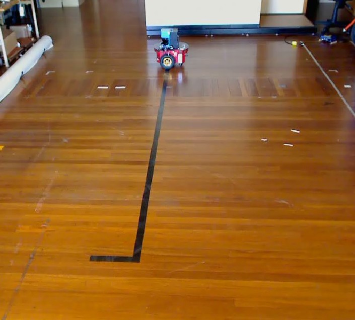
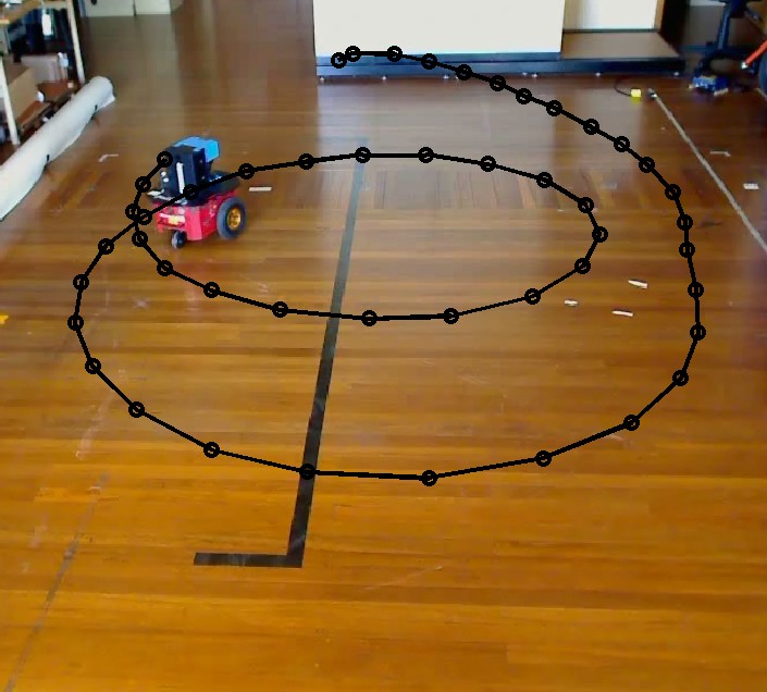
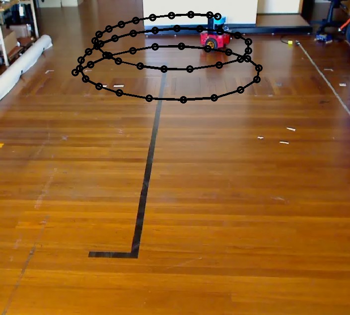
Figure 12.4: Sequence of images showing the experiment.

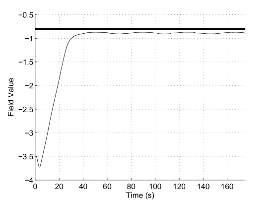
Figure 12.5: Evolution of the field value over the experiment. Field value is in metres.

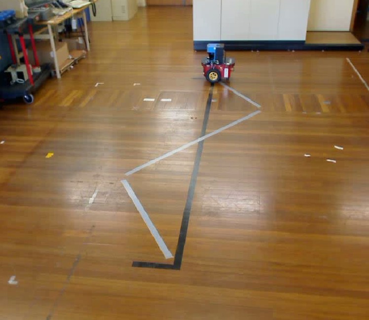
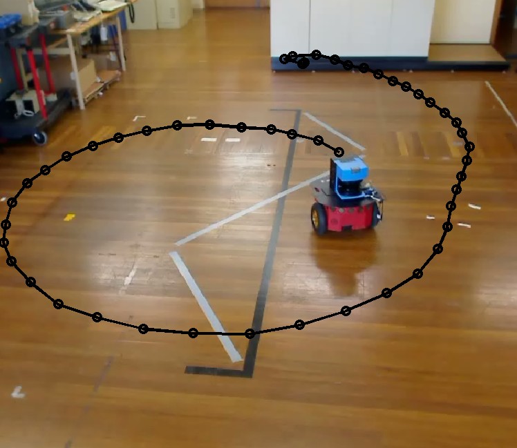
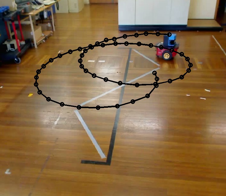
Figure 12.6: Sequence of images showing the experiment.

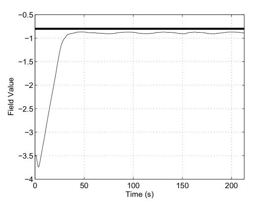
Figure 12.7: Evolution of the field value over the experiment. Field value is in metres.

12.7 Summary

The chapter presented a sliding-mode control law that drives a single non-holonomic Dubins-car like vehicle to the moving and deforming level curve of an unknown and time-varying scalar field distribution and ensures its ultimate circulation along this curve. The vehicle travels at a constant speed and is controlled by the turning radius; the sensor data are limited to the distribution value at the vehicle current location. This proposed control law does not employ gradient estimation and is non-demanding with respect to both motion and computation. Its performance was confirmed by computer simulations and experiments with real robots.

Chapter 13 Decentralized Target Capturing Formation Control

In this chapter a decentralized formation control problem is discussed, where the aim is to drive a group of vehicles into an equidistant formation along a circle, which is centred on a given target point. Sensor information is limited to scalar measurements about the target and surrounding vehicles. Simulations and experimental results are given to confirm the viability of the proposed method.

13.1 Introduction

A typical objective in multiagent systems research is to drive a team of vehicles to a pre-specified formation. Formation control is one of the basic technologies that enables multiple vehicles to cover large operational areas and accomplish complex tasks [297]. Although a rigorous stability analysis of such systems is generally an extremely hard task, partly due to time-varying topology of the information flows [95], some theoretical results have been obtained.

Recently, a substantial body of research was devoted to designs of control strategies that drive multiple vehicles to a capturing formation around a target object (see e.g. [211, 309, 212, 297, 160, 151, 298, 150, 86, 152, 159, 162, 354, 299, 335, 51, 125, 175]. This is motivated by various practical applications such as security and rescue operations, explorations in hazardous terrestrial or marine environments, deployments of mobile sensor networks, and patrolling missions using multiple unmanned vehicles [211, 212, 297]. In fact, the maneuver itself consists in enclosing and grasping. The former is to enclose the target object while approaching it, whereas the latter is to grasp the object by driving the vehicles to an optimal configuration around it, which is typically the equal spacing formation. Basically, the both objectives should be achieved in a decentralized fashion.

A decentralized capturing kinematic control law for multiple point-wise planar vehicles was proposed in [162]. This law follows the gradient decent approach and employs only local data at any agent (about the target and angularly closest neighbors). A distributed motion coordination strategy for multiple Hilare-type robots in cooperative hunting operations has been proposed and presents arguments supporting local stability of the closed-loop system [354].

Conditions have been established under which simple decentralized linear control laws can drive a team of identical linear planar fully actuated agents into a given target-centric formation [335]. However, the target is assumed to obey a known and favorable for the capturing task escaping rule, which is hardly realistic for most target-capturing scenario.

Several algorithms are inspired by the cyclic pursuit animal behavior [211, 309, 212]. Though the pure cyclic pursuit typically results in rendezvous for linear models, it was shown that in the nonlinear case (planar unicycle-like models), identical multiple vehicles can assemble a locally stable circular formation under certain circumstances [211, 212]. For non-identical unicycles and control gains, necessary conditions for the existence of a circular equilibrium have been obtained [309]. However, the resultant circle parameters (the center and radius) are not under control and are not related to a specific target, and not much was established about the global convergence of the proposed algorithms. By modifying the cyclic pursuit strategy, a distributed cooperative control scheme for capturing a target in 3D space by a team of velocity-controlled identical point-mass vehicles has been proposed [160]. This result was generalized for the case of under-actuated identical stable vehicles with common dynamics described by a linear MIMO model [159].

A serious limitation of all pursuit-based approaches is that they assume a fixed ring-like information-flow graph. More general and time-varying information-flow topologies have been examined, where a control strategy can proposed that drives a set of identical under-actuated planar unicycles into a cyclic formation [297]. However, the center of this formation is out of control and is not concerned with a particular target. Algorithms for enclosing a given moving target by a set of fully actuated planar kinematically controlled and identical but having an identity unicycles have been proposed for the case of general fixed communication topology with some special properties [151, 150]. This result was extended on a time-varying topology and kinematically controlled point-mass vehicles in 3D space [152] and planar dynamically controlled ones with inaccurate target information [299] or information exchange uncertainty [284]. The information graph may also be assumed independent of the control law, and the required properties are treated as granted [297, 151, 150, 152, 299]. However, in many cases this graph is determined by the current locations of the vehicles, along with their limited visibility or communication ranges, and so its properties essentially depend on the control laws driving the vehicles.

A scenario with position-dependent information graph has been considered for identical and indistinguishable kinematically controlled point-mass vehicles [125]. Each of them has access to the positions of the target and two neighbors, which are the angularly closest predecessor and follower in the circular order around the moving target, irrespective of their metric distances from the sensor. This does not match the capabilities of most sensors, for which the visibility of an object may essentially depend on this distance, whereas the angular discrepancy with respect to a third party (target) position does not matter.

All aforementioned works assume no limitations on both the control range and the distance sensible by the vehicle, which can hardly be qualified as realistic, and neglects the important issue of collision avoidance. Realistic models of sensors were examined in [51], where the visibility region of the vehicle is the union of a disc sector and a full disc of a smaller radius, which are associated with a narrow aperture long-distance sensor and an omnidirectional short distance one. For a steady target and a team of identical under-actuated unicycles with unlimited control ranges and full observation, including the mutual orientation of the vehicles, this approach proposes decentralized control laws and shows that they transform the desired uniform capturing configuration into a locally stable equilibrium of the closed-loop system. However, no rigorous results on global stability or collision avoidance are provided.

The issue of collision avoidance has also been addressed [86, 298, 175]. A control strategy has been proposed which drives a team of fully actuated unconstrained unicycles with all-to-all communication capability to a prescribed distance to a steady target, while avoiding collisions with each other [86]. However uniform distribution of the vehicles around the target is not ensured. A decentralized control rule was offered and shown to drive kinematically controlled and labeled point-mass unit-speed planar robots into an uniform circular formation around a steady beacon while avoiding collisions with each other and obstacles [298]. However, this rule handles the team with only three agents, which is a severe limitation. Another approach addresses both limited control range and collision avoidance [175]. This considers a team of identical and unlabeled unicycle-like planar vehicles and is basically focused on the capturing maneuver within a vicinity of a steady beacon, where the vehicles are assumed to acquire all-to-all visibility. The vehicles are kinematically controlled and fully actuated, with the ability to both stop, immediately reverse the direction of the motion, and track an arbitrarily contorted path. The proposed control strategy asymptotically steers the vehicles at the desired distance to the beacon and uniformly distributes them around it, with the speed of formation rotation about the beacon being unprescribed. Collision avoidance is guaranteed only if initially the vehicles lie on distinct rays issued from the target.

Thus the combination of realistic limited both control and sensor ranges was not addressed in the literature; moreover for realistic sensor models [51], no rigorous non-local convergence results were offered. Such results taking into account the issue of collision avoidance were established only for the team of three agents [298] or under the restricted assumption about the all-to-all communication [175]. Furthermore, all above references assume that both the line-of-sight angle (bearing) and the relative distance (range) of visible objects are available to the controller. However, the problem of range-only based navigation is critical for many areas such as wireless networks, unmanned vehicles and surveillance services [16, 104]. Many sensors typical for these areas, like sonars or range-only radars, provide only the relative distance between the sensor and the object. Range-only based navigation has a potential to reduce the hardware complexity and cost. However this benefit is undermined by the lack of suitable control design techniques.

In this chapter, a decentralized control strategy is described which drives a team of unlabeled and kinematically controlled planar non-holonomic Dubins-like vehicles into an equi-spaced circular formation at a given distance from a steady target. Unlike all papers in the area except for [175], the velocity range is limited, however unlike [175], the speed is not only upper but also lower bounded by a given constant so that the vehicle cannot stop or immediately reverse the direction of the motion. The speed lower bound provides an additional challenge since it causes restriction of the paths along which the vehicle can travel to the curves with upper limited curvatures. Another distinction from [175] is that the vehicles are not identical and the angular velocity of the formation rotation about the target is pre-specified.

The crucial difference of the approach described in this chapter from the entire previous research in the area is that first, the proposed navigation algorithm is based on range-only measurements; and second, the distance to a companion vehicle is accessible only when it lies within a given disc sector centered at the sensor (see Fig. 13.1(a)), which would hold for rigidly mounted narrow aperture distance sensors. It follows that dangerous sideways convergence of two vehicles may be undetectable by each of them, and this provides an additional challenge in design of the control law – it should exclude convergence in ‘invisible’ directions. It is assumed that the distance to the target is constantly available to any vehicle, which would hold if the target is endowed with a beacon facility or its visibility essentially exceeds that of the vehicles.

A sliding mode control strategy inspired by some ideas from [327] is proposed and shown to solve the problem. It may be proven via rigorous mathematical analysis that under some minor and partly unavoidable technical assumptions, the control objective is achieved without fail. It is possible to show that despite of range-only measurements, not only the required angular velocity but also the direction of the formation rotation about the target are ensured.

The applicability of the proposed controller is confirmed by computer simulations and experiments with real robots. In the extensive literature on the multi-vehicle coordination, real-world tests have been scarcely concerned up to now, especially with respect to the particular problem treated in this chapter. Accordingly, there is still considerable potential research that should be done on developing the practical aspects of these implementations. Such tests are particularly important since un-modeled system dynamics are a classical reason for control malfunction.

All proofs of mathematical statements are omitted here; they are available in the original manuscript [359].

The body of this chapter is organized as follows. In Sec. 13.2 the problem is formally defined, and in Sec. 13.3 the main analytical results are outlined. Simulations and experiments are presented in Secs. 13.4 and 13.5. Finally, brief conclusions are given in Sec. 13.6.

13.2 Problem Statement

In this chapter, a team of $N$ autonomous unicycle-like robots are considered, enumerated by $i\in[0:N-1]$. They travel in the plane with time-varying turning radii and longitudinal speeds limited by known constants; the speed is bounded from not only above but also below by positive constants. There also is a point-wise target or beacon $\boldsymbol{\mathscr{T}}$ in the plane. The objective is to drive all robots to the circle of the pre-specified radius $R$ centered at the target, to uniformly distribute them along this circle, and to maintain this formation afterwards. The number $N$ is known to every robot, and the formation should rotate with the prescribed angular velocity $\omega$.

To accomplish the mission, robot $i$ has access to the distance $d_{i\to\boldsymbol{\mathscr{T}}}$ from its center-point to the target. It also has access to the distance $d_{i}$ to the nearest companion robot among those from its visibility region. This is the sector between the arc and two radii of the circle of the given radius $r^{\text{vis}}_{i}>0$ centered at the robot, both radii are at the given angular distance $\lambda_{i}\in(0,\pi/2)$ from the forward centerline ray of the robot; see Fig. 13.1(a). Whenever there are no robots in this region, $d_{i}:=\infty$.

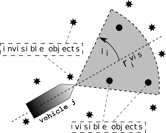
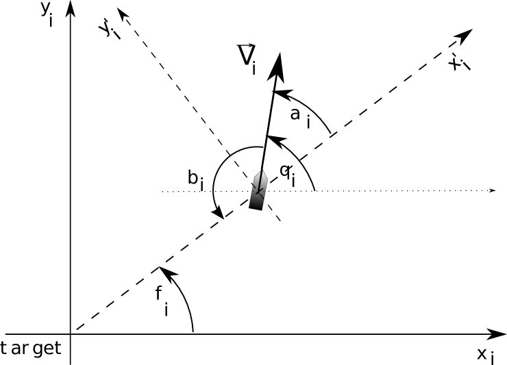
Figure 13.1: (a) The sensor capability of the robot; (b) Coordinate frames and variables; (c) The saturation function.

The following unicycle-like robot model is employed:

$$\begin{array}[]{r c l}\dot{x_{i}}&=&v_{i}\cos{\theta_{i}}\\ \dot{y_{i}}&=&v_{i}\sin{\theta_{i}}\end{array},\quad\begin{array}[]{l}\dot{\theta_{i}}=u_{i},\\ |u_{i}|\leq\overline{u}_{i},\underline{v}\,_{i}\leq v_{i}\leq\overline{v}_{i}.\end{array}$$ (13.1)

Here $x_{i},y_{i}$ are the Cartesian coordinates of the $i$th robot in the world frame centered at the target and $\theta_{i}$ gives the orientation of the robot (see Fig. 13.1(b)). The angular $u_{i}$ and longitudinal velocities $v_{i}$ are the controls; the bounds $\overline{u}_{i}>0,0<\underline{v}\,_{i}<\overline{v}_{i}$ are given. For the problem to be realistic, the required angular velocity $\omega$ of the formation rotation should be such that $\underline{v}\,_{i}\leq|\omega|R\leq\overline{v}_{i},|\omega|\leq\overline{u}_{i}$. This is slightly enhanced by assuming that:

$$\underline{v}\,_{i}<|\omega|R<\overline{v}_{i},\qquad|\omega|<\overline{u}_{i}\qquad\forall i.$$ (13.2)

To simplify the subsequent formulas, it is also assumed that the formation should rotate about the target counter-clockwise $\omega>0$.

In this chapter, the following simple switching control strategy is employed:

$$\left[\begin{array}[]{c}v_{i}\\ u_{i}\end{array}\right]:=\left[\begin{array}[]{c}\Psi_{i}(d_{i})\\ \overline{u}_{i}\text{\bf sgn}\left\{\dot{d}_{i\to\boldsymbol{\mathscr{T}}}+v_{i}\text{\bf sat}^{b_{i}}_{-b_{i}}\left[\big{(}m_{i}[d_{i\to\boldsymbol{\mathscr{T}}}-R]\big{)}\right]\right\}\end{array}\right].$$ (13.3)

Here the parameters $m_{i},b_{i}>0$ and the functions $\Psi_{i}(d)\in[\underline{v}_{i},\overline{v}_{i}]$ are chosen by the designer of the controller subject to requirements to be disclosed further.

The desired angular velocity $\omega$ of the formation will be taken into account by the requirements to $\Psi_{i}(\cdot)$. Note that the control law Eq.(13.3) produces only feasible controls $v_{i}\in\big{[}\underline{v}_{i},\overline{v}_{i}\big{]},|u_{i}|\leq\overline{u}_{i}$.

13.3 Summary of Main Results

In this section the control law Eq.(13.3) is demonstrated to achieve the control objective. This holds if apart from Eq.(13.2), another natural assumption is satisfied and the controller parameters are properly tuned:

Assumption 13.3.1

Under the uniform distribution over the required circle, every robot has at least one companion in its visibility region (see Fig. 13.2(a)):

$$\lambda_{i}>\Delta_{\ast}:=\frac{\pi}{N},\qquad r^{\text{vis}}_{i}>2R\sin\Delta_{\ast}.$$ (13.4)

To specify the choice of the speed gain functions $\Psi_{i}(\cdot)$ in Eq.(13.3), the following is introduced:

Definition 13.3.1

The function $g(\cdot)$ defined on $E\subset$ $[-\infty,+\infty]$ is said to be uniformly Hölder continuous is there exists $c\in[0,+\infty)$ and $\alpha\in(0,1]$ such that $|g(t^{\prime\prime})-$ $g(t^{\prime})|$ $\leq$ $c|t^{\prime\prime}-t^{\prime}|^{\alpha}$ for all $t^{\prime\prime},t^{\prime}\in E\cap\mathbb{R}$.

The choice of $\Psi_{i}(\cdot)$ proceeds from $\omega$ and two auxiliary velocity parameters $v_{i,\ast},v^{\ast}_{i}$ chosen so that:

$$\underline{v}_{i}\leq v_{i,\ast}<\omega R<v^{\ast}_{i}<\min\big{\{}\overline{u}_{i}R;\overline{v}_{i}\big{\}}.$$ (13.5)

Such choice is feasible thanks to Eq.(13.2). As $v_{i,\ast},v^{\ast}_{i}$ are picked, the choices of the controller parameters $\Psi_{i}(\cdot)$ and ($m_{i},b_{i}$) for the speed and steering gains, respectively, become independent of each other.

Requirement 13.3.1

The maps $\Psi_{i}(\cdot):[0,+\infty]\to[v_{i,\ast},v^{\ast}_{i}]$ are uniformly Hölder continuous and such that

1. $\Psi_{i}(d)=R\omega\;\forall d\in[0,d^{0}];\displaystyle{\inf_{d\geq d^{0}+\varepsilon}}\Psi_{i}(d)>R\omega\;\forall\varepsilon>0$, where $d^{0}:=2R\sin\frac{\pi}{N}$ is the distance between any two neighboring robots under their uniform distribution over the desired circle;

2. whenever $i\neq j$, the equation $\Psi_{i}(d)=\Psi_{j}(d)$ has no roots on $(d^{0},2R]$.

An example of the functions satisfying this requirement is as follows:

$$\Psi_{i}(d_{i}):=\text{\bf sat}^{v_{i}^{\ast}}_{v_{i,\ast}}\left[R\omega+k_{i}\left[d_{i}-2R\sin\frac{\pi}{N}\right]_{+}\right].$$ (13.6)

Here $[s]_{+}:=\max\{x,0\}$, whereas $k_{i}>0$ are tunable parameters and $k_{i}\neq k_{j}\;\forall i\neq j,\;k_{i}<k_{j}\Rightarrow v_{i}^{\ast}<v_{j}^{\ast}.$

The proposed controller in fact employs the reduced speed range $[v_{i,\ast},v^{\ast}_{i}]\subset[\underline{v}_{i},\overline{v}_{i}]$. As will be shown, the closer this range to $\omega R$, the larger the estimated convergence domain.

The choice of the steering gain parameters is subjected to the following limitations:

$$0<b_{i}<1,\qquad 0<m_{i}<\frac{\sqrt{1-b_{i}^{2}}}{b_{i}}\left[\frac{\overline{u}_{i}}{v^{\ast}_{i}}-\frac{1}{R}\right]\qquad i\in[0:N-1],$$ (13.7)

Here the right-hand side of the last inequality is positive due to the last inequality from Eq.(13.5). Such choice is always possible – chosen $b_{i}$, all small enough $m_{i}$ are feasible.

To state the main results of the chapter, the rotating normally oriented Cartesian frame RCF_i is introduced, which is centered at the target with the abscissa axis directed towards robot $i$ (see Fig. 13.1(b)). Let $\varphi_{i}$ stand for the angle from the abscissa axis of the world frame to that of RCF_i, with the anticlockwise angles being positive. The correct behaviour of the system is defined as follows:

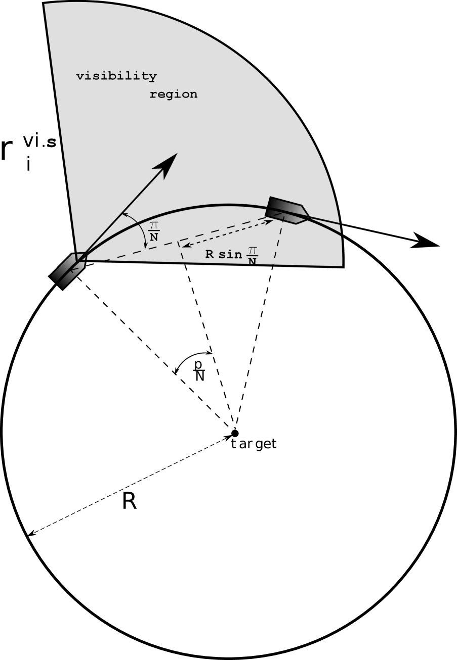
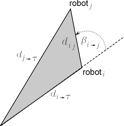
Figure 13.2: (a) Visibility region under uniform distribution; (b) Relative polar coordinates.

Definition 13.3.2

The cumulative trajectory of the team of $N$ robots is said to be target capturing if

$$d_{i\to\boldsymbol{\mathscr{T}}}(t)\to R,\qquad\dot{\varphi_{i}}(t)\to\omega\ \quad\text{\rm as}\quad t\to\infty\quad\forall i\in[0:N-1],$$ (13.8)

vehicle-to-target collisions are excluded $d_{i\to\boldsymbol{\mathscr{T}}}(t)>0\;\forall t,i$, and the robots can be enumerated so that

$$\varphi_{i\oplus 1}(t)-\varphi_{i}(t)\to 2\Delta_{\ast}=\frac{2\pi}{N}\quad\text{\rm as}\quad t\to\infty.$$ (13.9)

Here and throughout $\oplus$ denotes the addition modulus $N$. It is underscored that this enumeration should be static – it does not alter as time progresses.

The following theorem is the first main result of the chapter:

Theorem 13.3.1

Suppose that Assumption 13.3.1 and Eq.(13.2) hold and the controller parameters satisfy Requirement 13.3.1 and Eq.(13.7). Then the control law Eq.(13.3) gives rise to a target capturing trajectory whenever the robots are initially far enough from the target:

$$d_{i\to\boldsymbol{\mathscr{T}}}(0)>4r^{\ast}_{i}-2r_{i,\ast}+\frac{1}{\frac{1}{r^{\ast}_{i}}-\frac{m_{i}b_{i}}{\sqrt{1-b_{i}^{2}}}}\quad\forall i\in[0:N-1],\quad\text{\rm where}\quad r^{\ast}_{i}:=\frac{v^{\ast}_{i}}{\overline{u}_{i}},r_{i,\ast}:=\frac{v_{i,\ast}}{\overline{u}_{i}}.$$ (13.10)

Theorem 13.3.1 ignores the issue of possible collisions between the vehicles. It is tacitly taken for granted that the collisions are resolved by an extra controller. Moreover, this controller does not essentially corrupt the trajectories implemented under the proposed control law. However, under a mild additional assumption, the proposed control strategy automatically prevents inter-vehicle distance converging to zero:

Proposition 13.3.1

Suppose that the assumptions of Theorem 13.3.1 are true, the gain coefficients $m_{i},b_{i}$ in Eq.(13.3) are taken common for all robots, and the initial distance $d_{ij}(0)$ between any pair of robots $i\neq j$ is large enough

$$d_{ij}(0)>3\pi(\overline{v}_{i}+\overline{v}_{j})\max_{\nu=1,\ldots,N}\overline{u}_{\nu}^{\,-1}.$$ (13.11)

Then the inter-vehicle collisions are excluded: $d_{ij}(t)>0\;\forall t,i$.

13.4 Simulations

To verify the correct operation of the proposed control law, the system was simulated in a range of scenarios. The control was updated with a sampling period of 0.01 s. The vehicle and controller parameters are shown in Table 13.1. The closed loop trajectories for each vehicle are shown in Fig. 13.3, which displays the expected behavior of the vehicles: they converge to the desired circle around the target, while equalizing the inter-vehicle distances.

$\omega$	$\frac{\pi}{8}rads^{-1}$
$R$	$3m$
$\overline{u}_{i}$	$1.5rads^{-1}$

$k_{i}$	$10s^{-1}$
$v_{i}^{*}$	$3ms^{-1}$
$v_{i,*}$	$2ms^{-1}$

$m_{i}$	$2m^{-1}$
$b_{i}$	$0.5$

$\lambda_{i}$	$\frac{\pi}{2}rad$
$r_{i}^{vis}$	$10m$

Table 13.1: Simulation parameters for target-capturing controller.

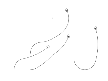
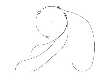
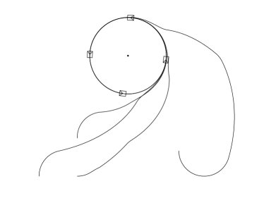
Figure 13.3: Simulations with four vehicles converging to equal spacing around a target.

This is confirmed by Figures 13.4 and 13.5. The first of them shows that the distance from each vehicle to the target converges to the prescribed value $3m$. The initial orientation of the vehicle determines whether this convergence is monotonic or not - the vehicle initially oriented away from the target unexpectedly experiences a temporary increase in the target distance, while the others do not. Fig. 13.5 shows that eventually the angle subtended around the target increases at nearly the desired rate $\omega=\frac{\pi}{8}rads^{-1}$, with nearly equal spacing between vehicles.

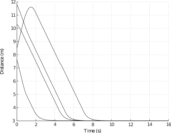
Figure 13.4: Distance to the target for each of the four vehicles in Fig. 13.3.

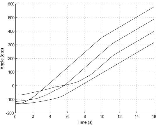
Figure 13.5: Angle subtended from the target for each of the four vehicles in Fig. 13.3.

The system was also tested in a situation where the target moves. Though this case is not covered by Theorem 13.3.1, Fig. 13.6 demonstrates that the control law still ensures the desired behavior. Since the target is slowly moving to the left, the final paths of the vehicles unexpectedly resemble cycloids.

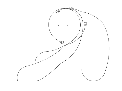
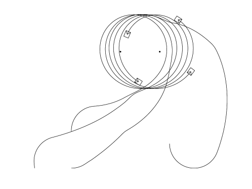
Figure 13.6: Simulations with enclosing and grasping of a moving target.

The choice Eq.(13.6) of the function $\Psi_{i}(d_{i})$ in the control law Eq.(13.3) assumes that the team size $N$ is known. If this size is unknown, the control law can be modified so that this information is not required:

$$\Psi_{i}(d_{i}):=\text{\bf sat}^{v_{i}^{\ast}}_{v_{i,\ast}}\left[kd_{i}\right]$$ (13.12)

Contrary to Eq.(13.6), the gain $k$ is common for all vehicles here. Theoretical analysis of this control law, including recommendations on the choice of the controller parameters, is outside of the scope of this discussion and is a topic of ongoing research. For this preliminary simulation testing of this law, the parameters used in the test are given in Table 13.2. Simulations showed that the system still behaves in a similar manner as before: the vehicles converge to the desired circle centered at the target, while equalizing the inter-vehicle spacing. A typical simulation result is shown in Figure 13.7, where initially three vehicles converge to an uniform formation, which is proceeded by an extra vehicle joining the team, causing rearrangement of the uniform formation.

$k$	$0.25s$
$v_{i}^{*}$	$4ms^{-1}$
$v_{i,*}$	$1ms^{-1}$

$m_{i}$	$1m^{-1}$
$b_{i}$	$0.125$

Table 13.2: Simulation parameters for target-capturing with unknown team size.

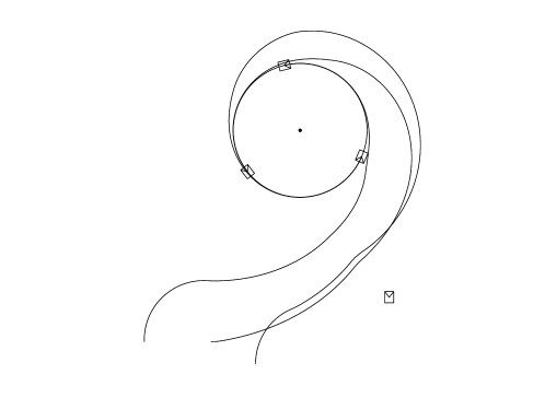
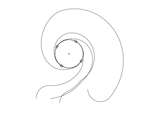
Figure 13.7: Simulations with addition of vehicles during the target capturing maneuver.

13.5 Experiments

Experiments were carried out with three pioneer P3-DX mobile robots to show real-time applicability of the proposed control system. A SICK LMS-200 laser range-finding device was used to detect the vehicles and target. This device has a nominal accuracy of $15mm$ along each detection ray, however the accuracy may be significantly worse in real world circumstances. The range sensor was rotated 45 deg to the left to provide a better view of the target. The algorithm for determining the position of the target and companion vehicles is as follows:

• The detected points were segmented into clusters by identifying consecutive detection points with an Euclidean separation smaller than $0.2m$. The resultant sequence of points was filtered based on the distance between the edges of the cluster. In the experiment, the cutoff was set so that the cluster diameter was between $0.1m$ and $0.4m$.

• The distance from the vehicle to the cluster was taken to be the distance along the detection ray bisecting the edges of the cluster. The clusters were filtered based on this distance and a cutoff was set so that this measurement was under $3m$ in the experiment. The closest cluster was taken to be the target, and the next closest cluster to the right of the target was taken to be the next vehicle.

At each control update, the speed and turning rate of the low level wheel controllers were set in accordance with the output of the navigation algorithm. The control was updated with a period of $0.2s$. The values of the parameters used in the experiments are listed in Fig. 13.3.

It is common to implement chattering reduction in sliding mode control systems by smooth approximation of the signum function, and this can be achieved using a linear function with saturation. However this may cause static error of the turning rate, thus entailing a tracking error. As an alternative, the steering control (commissioned to navigate the robot to the desired distance to the target point) was approximated by replacing $\overline{u}_{i}\text{\bf sgn}$ in the second line from Eq.(13.3) by the function from Figure 13.8, where $S_{\max}$ is an upper estimate of the absolute value of the function in the curly brackets from Eq.(13.3) in the domain where this function is negative and the concerned sat is not saturated. In this experiment, $S_{\max}$ was taken to be $1.0ms^{-1}$. According to Figure 13.8, this uniquely determines the slope of the function on the negative ray of the abscissa axis; on the positive ray, the slope is the same. Such choice does not influence the equilibrium turning rate, thus eliminating the above static error issue.

Figure 13.8: Saturation function used to reduce chattering during the experiment.

$N$	3
$\overline{u}_{i}$	$1.5rads^{-1}$
$\lambda_{i}$	$\frac{\pi}{2}$

$r_{i}^{vis}$	$10m$
$v_{i}^{*}$	$0.1ms^{-1}$
$v_{i,*}$	$0.2ms^{-1}$

$\omega$	$\frac{\pi}{25}rads^{-1}$
$R$	$1m$

$k_{i}$	$0.06s^{-1}$
$m_{i}$	$0.2m^{-1}$
$b_{i}$	$0.05$

Table 13.3: Experimental parameters for target-capturing controller.

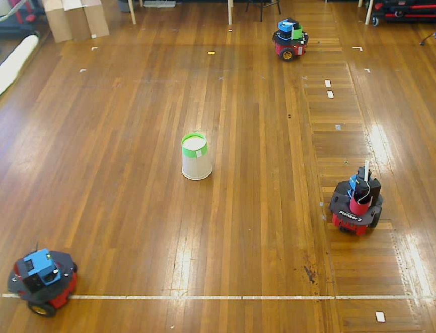
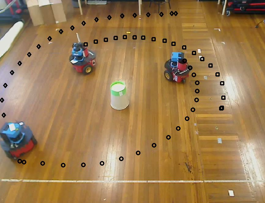
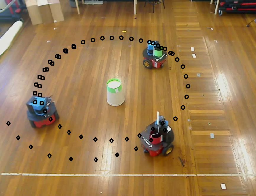
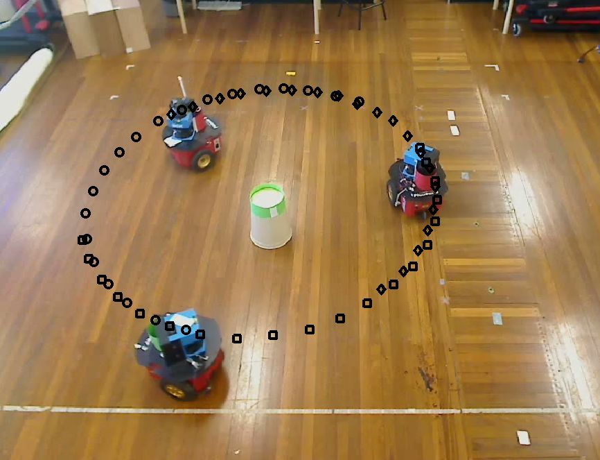
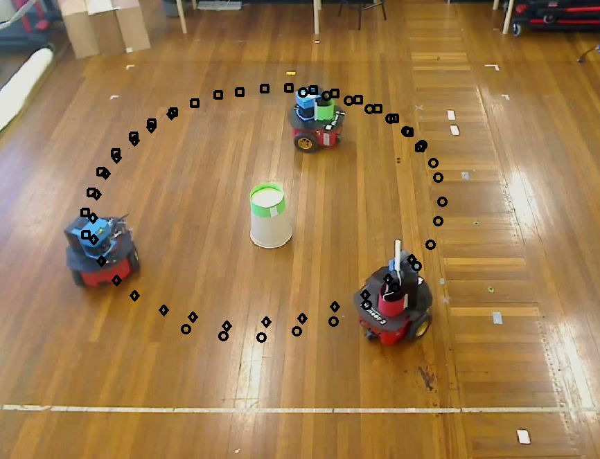
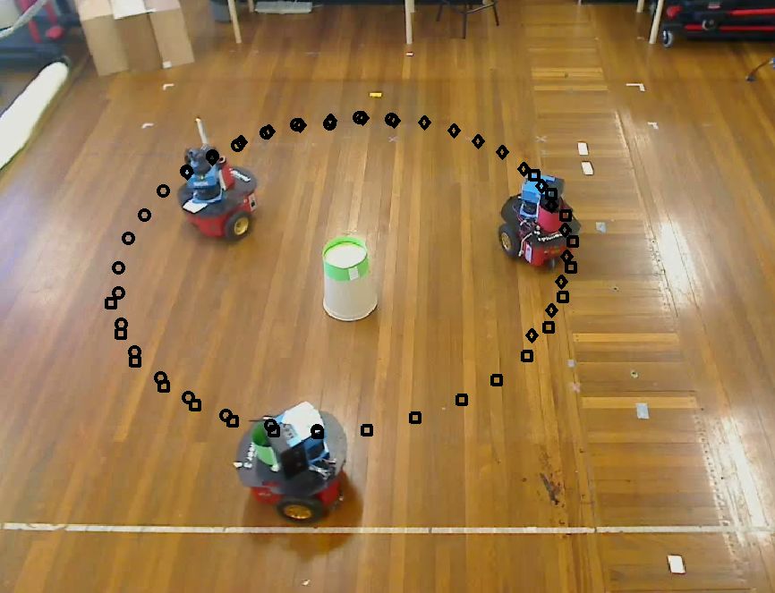
Figure 13.9: Sequence of images showing the experiment.

Figure 13.10: Distance to the center during the experiment.

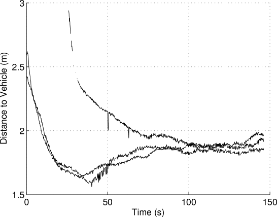
Figure 13.11: Distance to the nearest visible robot.

A sequence of images obtained during the experiment is shown in Fig. 13.9, where the positions of the robots were manually marked in the video frames. Figures 13.10 and 13.11 demonstrate convergence to the required formation and confirm real-life applicability of the proposed control law.

13.6 Summary

In this chapter the problem of capturing a target using a team of decentralized non-holonomic vehicles was investigated, where the objective is to drive all vehicles to the circle of the prescribed radius centered at the target with uniform separation. If every vehicle has access to the distance to the target and the distances to the companions from the given disc sector centered at this vehicle, it may be shown that the objective is achieved. The performance of the control law is illustrated by computer simulations and experiments with real robots.

Chapter 14 Conclusions

This report is concerned with provable collision avoidance of multiple autonomous vehicles operating in unknown environments. The main contributions of this work are a novel MPC-based strategy applicable to multiple vehicle systems (see Chapt. 5), along with an approach to navigation problems where information about the obstacle is described by a ray-based sensor model (see Chapt. 4).

The decentralized coordination of multiple vehicle systems is a relatively recent area of research, and the approach described in this report provides some advantages over other proposed solutions to this problem. In particular it allows vehicles to simultaneously update trajectories, use a sign-board based communication model, and avoid artificial limitations to the magnitude of trajectory alterations. Through it currently only works with simplified planning algorithms of the type proposed in Chapt. 3, it seems to be a useful approach for practical implementations in vehicles.

Concurrent use of both a ray-based sensor model, and a realistic vehicle kinematic model to achieve boundary following has been previously proposed, but is limited to the use of a single detection ray. The application of MPC to boundary following problems proposed in this report is original, and has many desirable properties such as adaptable speed and offset distance. Additionally, while assumptions about the obstacle are unavoidable, these are likely more general than previously proposed approaches. It seems that combined sensor and MPC-based navigation is an approach which could be useful for many applications in the future.

An additional contribution of this work is a proposed extension to allow deadlock avoidance in Chapt. 6. While only applicable to only two vehicles, the proposed idea is novel since all previously proposed deadlock avoidance systems either rely on intractable centralized coordination, discrete graph-based state abstractions, or an obstacle free workspace. Showing local deadlock avoidance for even two vehicles seems to be a useful property for a navigation law.

The local reactive navigation strategy proposed in Chapt. 3 is based on a combination of simplified planning algorithms and robust MPC, and some of the details involved make it original. The method is applicable to both holonomic and unicycle vehicle models with bounded acceleration and disturbance. Many simulations and real world tests throughout this report confirm the viability of the proposed methods. While Chapts. 3 to 6 are all based on the same basic control structure, solving a generalised problem with multiple vehicles and limited sensor data was not attempted, and this would be the logical next step to extend this work.

In most cases analytical justification for showing the correct behavior of the proposed methods was offered. This type of justification is becoming increasing important in robotics research. Properties such as provable collision avoidance under disturbance are generally only easily provable using robust MPC, however these often require significant computation and communication capabilities, making real time use more difficult. This is especially apparent in the development of micro UAV vehicles, which have limited resources available. It is hoped the approaches described in this report provide a suitable trade-off between tractability, optimality and robustness.

In addition to collision avoidance, task achievement is a desirable attribute to prove. In Chapt. 4 complete transversal of the obstacle and finite completion time is shown. If high level navigation system functions can be delegated to low level controllers without significant complication, it may increase the overall durability of the system (it seems likely that high level decision making system are slower and more likely to fail in the real world).

Lastly, Chapts. 7 to 13, provide simulations and real world testing performed to validate a variety of other navigation systems. The contributions are listed as follows:

• Chapt. 7 solves the problem of reactively avoiding obstacles and provably converging to a target using very limited scalar measurements. The advantage of the proposed method is that it can be analytically shown to have the correct behavior, despite the extremely limited sensor information assumed to be available.

• Chapt. 8 provides a method for reactively avoiding obstacles and provably converging to a target using a tangent sensor. The advantage of the proposed method is that it explicitly allows for the kinematics of the vehicle.

• Chapt. 9 achieves a method for path following with side slip allowance suitable for an agricultural vehiclele. The advantage of the proposed method is that it explicitly allows for steering angle limits, and it has been shown to have good comparative performance in certain situations.

• Chapt. 10 contributes a method which allows the boundary of an obstacle to be followed using only a rigid range sensor. The advantage of the proposed method is that it provides a single contiguous controller, and is analytically correct at transitions from concave to convex boundary segments.

• Chapt. 11 provides a novel method for seeking the maximal point of a scalar environmental field. The advantage of the proposed method is that it des not require any type of derivative estimation, and it may be analytically proven to be correct in the case of time–varying environmental fields.

• Chapt. 12 achieves a new approach of tracking level sets of an environmental field. The advantage of the proposed method is that it may be analytically proven to be correct in the case of time–varying environmental fields.

• Chapt. 13 achieves a novel method of decentralized formation control for a group of robots. The advantage of the proposed method is that it only requires local sensor information, allows for vehicle kinematics and does not require communication between vehicles.

Future Work

The work in this report opens up a number of future research problems as follows:

• Deadlock avoidance. In Chapt. 6, the deadlock avoidance problem for a pair of vehicles was explored. While an approach applicable to an arbitrary number of vehicles would extremely non-trivial, it remains an open question as to whether decentralized MPC approaches can be extended to cover this case. Also, a version which do not require the use of a navigation function could be useful, through this may rely on Bug type behavior and would complicate analysis.

• Broader robustness analysis. Noise and model disturbance was not considered in Chapts. 4 or 6. Through it may complicate the analysis, employing the full robust MPC technique from Chapt. 3 should be possible.

• Navigation system unification. Currently the navigation system in Chapts. 5 and 6 has not been unified with the navigation system in Chapt. 4. A system which coordinates multiple vehicles while taking sensor constraints into account may be possible, however it may complicate subsequent analysis.

• Trajectory planning heuristic. When designing incomplete trajectory planning systems, the design of the set of possible trajectories is largely heuristic, and could be tuned for better performance. A wider range of possible trajectory shapes has previously been considered [37], through there is no evidence this is the best possible choice. A possible avenue of research would be to apply some global optimization method to determine the best possible set of trajectories to consider for a particular class of scenarios. One possible advantage is that the trajectory planner may favor vehicle positions which provide a marginally more informative view of the obstacle.

• Extensions to 3D. There is no reason why the navigation framework presented here cannot be extended to a three dimensional workspace. In these cases the tractability of the trajectory planner becomes a much more critical issue, so simplified planning approaches would be well suited to this problem.

• Other navigation tasks. A highly active area of research currently is formation control of a group of vehicles [350]. The multiplexed MPC framework was recently extended to achieve collision avoidance, successfully achieving decentralized, robust formation control [350]. It may be possible to extend the approach proposed in Chapt. 3 to formation control problems, while retaining the relevant advantages.

• Potential field methods for acceleration bounded vehicles. As mentioned in Chapt. 2, the problem of achieving collision avoidance using an APF method for acceleration bounded vehicles has not been fully solved. Through it seems unlikely an APF method would achieve the same closed loop performance as MPC, solution to this problem may be useful to provide more objective comparisons between the methods.

Chapter 15 Simulations with a Realistic Helicopter Model

This appendix outlines preliminary simulations that were carried out with a realistic helicopter model.

15.1 Helicopter Model

In order to further test the proposed navigation approach, the basic navigation approach was also tested against a realistic helicopter model [107, 106]. The helicopter model is based on an autonomous 8.2 kg helicopter with a main rotor diameter of $1.52m$, based on a Hirobo Eagle helicopter with conventional main rotor and tail rotor configuration. The Eagle, described further in [7] is electrically propelled and instrumented with differential GPS, Inertial Measurement Unit and an on-board autopilot.

The simulation combines a linearized rotor aerodynamic model with non-linear rigid body equations. A non-linear thrust and rotor inflow model is also incorporated, involving an iterative scheme to simultaneously solve for the induced down wash velocity through the rotor and the corresponding thrust. This approach produces a minimum complexity model which captures the essential dynamics of the helicopter. Balancing simulation fidelity against practicality, a simulation has been created that is capable of simulating the following effects:

• Exact non-linear rigid body equations of motion;

• Wind gusts and turbulence;

• First order main rotor flapping dynamics;

• Hover, rear-wards, sideways and forward flight;

• Dynamic effects of the Bell-Hiller stabilizer bar;

• Fuselage and tail-plane aerodynamic forces;

• Approximate servo dynamics; and

• Sensor lags, filtering, offsets and noise.

The main rotor forces and moments are controlled by the collective and cyclic pitch channels. The collective pitch control varies the average blade incidence of all of the blades. Increasing the collective pitch control results in an increased angle of attack of each blade and a subsequent increase in main rotor thrust. Decreasing the collective pitch has the opposite effect. The vertical motion of the helicopter is thus controlled by varying the collective pitch.

In order to achieve pitching and rolling moments, the orientation or tilt of the rotor disk is changed by applying pitch that varies cyclically, once per revolution. Increasing the blade pitch on one side of the rotor disk and decreasing it on the opposite side causes the path of the blade tips, known as the Tip Path Plane (TPP) to be tilted. Since the thrust vector acts essentially perpendicular to the TPP, this can be used to change the trim of the helicopter.

To simplify debugging, the simulation is divided into a number of blocks and subsystems. On the highest level, the simulation consists of an aerodynamics subsystem, sensor subsystem, sensor fusion block and controller subsystem as shown in Fig. 15.1. Most of the computational blocks have been implemented as C code S-functions. A detailed discussion on the principles behind this model can be found in [106].

Initial adjustments of the simulation were made to match the trim control settings of the simulation to the collective pitch, aileron and elevator settings observed from flight test. The simulation was validated against actual flight test data using frequency response techniques based on chirp and doublet waveforms.

A commonly used scheme for controlling a helicopter is used for this part of the controller and consists of an attitude feedback inner loop implemented as a PD controller, combined with a PI based velocity outer loop. This scheme effectively deals with the problem of the helicopter being under-actuated. In the inner loop, cyclic pitch is used to control the helicopter pitch and roll attitude. For the outer loop controller, the desired pitch and roll attitude is set in response to the velocity error using PI feedback.

The gains were tuned systematically using trial and error to converge on an acceptable solution. In the first instance, the attitude control loop was tuned independently by turning off the outer loop and stopping the integration of velocity and position in the dynamics block. Once satisfactory stability was demonstrated, the outer loop was re-activated and the velocity gains were then tuned.

The main inputs to this system are the desired velocities in the longitudinal and lateral directions, and the desired heading. Height and heading were controlled using separate PID control of collective pitch and tail rotor pitch respectively. A constant height above ground was maintained by the collective pitch PID controller.

15.2 Testing

To interface the proposed navigation law with the low level controllers in the helicopter model, the desired velocity in the longitudinal and lateral directions were set to $[v_{long},$ $v_{lat}]$ $=$ $R(-\theta(k))\cdot v^{*}(1|k)$, where $R(\cdot)$ is the $2\times 2$ rotation matrix converting the coordinates from the world frame to the relative helicopter reference frame. The desired heading was set to $\theta(1|k)$.

Figure 15.1: Block view of the helicopter model under test.

For all these simulations, the controller refresh rate of 5 Hz was used. The parameters used for control can be found in Table 15.1.

$u_{max}$	$1.9ms^{-2}$
$u_{p}$	$1.5ms^{-2}$
$u_{sp}$	$1.0ms^{-2}$

$d_{tar}$	$5m$
$v_{max}$	$4.5ms^{-1}$
$\gamma_{0}$	$10$

Table 15.1: Simulation parameters for collision avoidance with a realistic helicopter vehicle model.

Figure 15.2: Simulations with a realistic helicopter model.

Fig. 15.2 indicates the simulated helicopter was successfully able to navigate a cluttered environment using the proposed method. This introductory experiment gives promising results for using the proposed method to navigate real world helicopters.

Bibliography

- [1] Y. Abe and M. Yoshiki. Collision avoidance method for multiple autonomous mobile agents by implicit cooperation. In Proceedings of the IEEE/RSJ International Conference on Intelligent Robots and Systems, volume 3, pages 1207–1212, Maui, HI, USA, 2001.
- [2] H. Abelson and A. A. diSessa. Turtle Geometry. MIT Press, Cambridge, 1980.
- [3] P. Abichandani, G. Ford, H. Y. Benson, and M. Kam. Mathematical programming for multi–vehicle motion planning problems. In Proceedings of the IEEE International Conference on Robotics and Automation, pages 3315–3322, St Paul, MN, USA, 2012.
- [4] S. Adinandra, E. Schreurs, and H. Nijmeijer. A practical model predictive control for a group of unicycle mobile robots. In Proceedings of the 4th IFAC Conference on Nonlinear Model Predictive Control, volume 4, pages 472–477, Leeuwenhorst, Netherlands, 2012.
- [5] S. K. Agrawal and J. C. Ryu. Trajectory planning and control of a car–like mobile robot with slip using differential flatness. In Proceedings of the International Conference on Robotics and Automation, Pasadena, CA, USA, 2008.
- [6] M. A. Ahmadi-Pajouh, F. Towhidkhah, S. Gharibzadeh, and M. Mashhadimalek. Path planning in the hippocampo–prefrontal cortex pathway: An adaptive model based receding horizon planner. Medical Hypotheses, 68(6):1411–1415, 2007.
- [7] B. Ahmed, H. R. Pota, and M. Garratt. Flight control of a rotary wing UAV–a practical approach. In Proceedings of the 47th IEEE Conference on Decision and Control, pages 5042–5047, Cancun, Mexico, 2008.
- [8] M. Alamir and N. Marchand. Constrained minimum–time–oriented feedback control for the stabilization of nonholonomic systems in chained form. Journal of Optimization Theory and Applications, 118(2):229–244, 2003.
- [9] A. Albagul and Wahyudi. Dynamic modeling and adaptive traction control for mobile robots. In Proceedings of the 30th Annual Conference of IEEE Industrial Electronics Society, volume 1, pages 614–620, Busan, Korea, 2004.
- [10] J. Alonso-Mora, A. Breitenmoser, P. Beardsley, and R. Siegwart. Reciprocal collision avoidance for multiple car–like robots. In Proceedings of the 2012 IEEE International Conference on Robotics and Automation, pages 360–366, St Paul, MN, USA, 2012.
- [11] D. Althoff, J. Kuffner, D. Wollherr, and M. Buss. Safety assessment of robot trajectories for navigation in uncertain and dynamic environments. Autonomous Robots, 32(3):285–302, 2012.
- [12] J. C. Alvarez, A. Shkel, and V. Lumelsky. Accounting for mobile robot dynamics in sensor–based motion planning: experimental results. In Proceedings of the IEEE International Conference on Robotics and Automation, volume 3, pages 2205–2210, Lueven, Belgium, 1998.
- [13] S. B. Andersson. Curve tracking for rapid imaging in AFM. IEEE Transactions on Nanobioscience, 6(4):354–361, 2007.
- [14] L. Armesto, V. Girbes, M. Vincze, S. Olufs, and P. Munoz-Benavent. Mobile robot obstacle avoidance based on quasi–holonomic smooth paths. In Advances in Autonomous Robotics, volume 7429 of Lecture Notes in Computer Science, pages 244–255. Springer Berlin–Heidelberg, 2012.
- [15] V. I. Arnold. The Theory of Singularities and its Applications. The Press Syndicate of the University of Cambridge, Cambridge, second edition, 1993.
- [16] A. Arora, P. Dutta, and S. Bapat. A line in the sand: A wireless sensor network for target detection, classification, and tracking,. Computer Networks, 45(6):605–634, 2004.
- [17] R. Bachmayer and N. E. Leonard. Vehicle networks for gradient descent in a sampled environment. In Proceedings of the 41st IEEE Conference on Decision and Control, pages 113–117, Las Vegas, NV, USA, 2002.
- [18] R. Balakrishna and A. Ghosal. Modeling of slip for wheeled mobile robots. IEEE Transactions on Robotics and Automation, 11(1):126–132, 1995.
- [19] D. J. Balkcom, P. A. Kavathekar, and M. T. Mason. Time–optimal trajectories for an omni–directional vehicle. The International Journal of Robotics Research, 25(10):985–999, 2006.
- [20] C. Barat and M. J. Rendas. Benthic boundary tracking using a profiler sonar. In Proceedings of the IEEE/RSJ International Conference on Intelligent Robots and Systems, volume 1, pages 830–835, Las Vegas, NV, USA, 2003.
- [21] D. Baronov and J. Baillieul. Reactive exploration through following isolines in a potential field. In Proceedings of the American Control Conference, pages 2141–2146, New York, NY, USA, 2007.
- [22] D. Baronov and J. Baillieul. Autonomous vehicle control for ascending/descending along a potential field with two applications. In Proceedings of the American Control Conference, pages 678–683, Seattle, WA, USA, 2008.
- [23] K. E. Bekris, D. K. Grady, M. Moll, and L. E. Kavraki. Safe distributed motion coordination for second–order systems with different planning cycles. The International Journal of Robotics Research, 31(2):129–150, 2012.
- [24] K. E. Bekris, K. I. Tsianos, and L. E. Kavraki. Safe and distributed kinodynamic replanning for vehicular networks. Mobile Networks and Applications, 14(3):292–308, 2009.
- [25] F. Belkhouche. Reactive path planning in a dynamic environment. IEEE Transactions on Robotics, 25(4):902–911, 2009.
- [26] C. Belta, A. Bicchi, M. Egerstedt, E. Frazzoli, E. Klavins, and G. J. Pappas. Symbolic planning and control of robot motion [grand challenges of robotics]. IEEE Robotics Automation Magazine, 14(1):61–70, 2007.
- [27] C. Belta, V. Isler, and G. J. Pappas. Discrete abstractions for robot motion planning and control in polygonal environments. IEEE Transactions on Robotics, 21(5):864–874, 2005.
- [28] A. Bemporad and D. Barcelli. Decentralized model predictive control. Lecture Notes in Control and Information Sciences, 406:149–178, 2010.
- [29] A. Bemporad, M. D. Marco, and A. Tesi. Sonar–based wall–following control of mobile robots. ASME Journal of Dynamic Systems, Measurement and Control, 122(1):226–230, 2000.
- [30] S. Bereg and D. Kirkpatrick. Curvature–bounded traversals of narrow corridors. In Proceedings of the 21st Annual Symposium on Computational Geometry, pages 278–287, Pisa, Italy, 2005.
- [31] A. L. Bertozzi, M. Kemp, and D. Marthaler. Determining environmental boundaries: Asynchronous communication and physical scales. In V. Kumar, N. E. Leonard, and A. S. Morse, editors, Cooperative Control, pages 25–42. Springer–Verlag, Berlin, 2004.
- [32] E. Besada-Portas, L. de la Torre, J. M. de la Cruz, and B. de Andres-Toro. Evolutionary trajectory planner for multiple UAVs in realistic scenarios. IEEE Transactions on Robotics, 26(4):619–634, 2010.
- [33] G. Bevan, H. Gollee, and J. O’reilly. Automatic lateral emergency collision avoidance for a passenger car. International Journal of Control, 80(11):1751–1762, 2007.
- [34] A. Bicchi, G. Casalino, and C. Santilli. Planning shortest bounded–curvature paths for a class of nonholonomic vehicles among obstacles. Journal of Intelligent and Robotic Systems, 16(4):387–405, 1996.
- [35] E. Biyik and M. Arcak. Gradient climbing in formation via extremum seeking and passivity–based coordination rules. In Proceedings of the 46th IEEE Conference on Decision and Control, pages 3133–3138, New Orleans, LA, USA, 2007.
- [36] L. Blackmore, M. Ono, and B. C. Williams. Chance–constrained optimal path planning with obstacles. IEEE Transactions on Robotics, 27(6):1080–1094, 2011.
- [37] J.-L. Blanco, J. Gonzalez, and J.-A. Fernandez-Madrigal. Extending obstacle avoidance methods through multiple parameter–space transformations. Autonomous Robots, 24(1):29–48, 2008.
- [38] A. M. Bloch. Nonholonomic mechanics and control. Springer–Verlag, NY, 2003.
- [39] N. W. Bode, A. J. Wood, and D. W. Franks. Social networks and models for collective motion in animals. Behavioral Ecology and Sociobiology, 65(2):117–130, 2011.
- [40] F. Bonin-Font, A. Ortiz, and G. Oliver. Visual navigation for mobile robots: A survey. Journal of Intelligent and Robotic Systems, 53(3):263–296, 2008.
- [41] V. Boquete, R. Garcia, R. Barea, and M. Mazo. Neural control of the movements of a wheelchair. Journal of Intelligent and Robotic Systems, 25(3):213–226, 1999.
- [42] S. Bouraine, T. Fraichard, and H. Salhi. Provably safe navigation for mobile robots with limited field–of–views in dynamic environments. Autonomous Robots, 32(3):267–283, 2012.
- [43] R. W. Brockett. Asymptotic stability and feedback stabilization. In R. W. Brockett, J. Millmann, and H. Sussman, editors, Differential Geometric Control Theory, pages 181–191. Birkhauzer, Boston, 1983.
- [44] A. Brooks, T. Kaupp, and A. Makarenko. Randomised MPC–based motion–planning for mobile robot obstacle avoidance. In Proceedings of the 2009 IEEE International Conference on Robotics and Automation, pages 397–402, Kobe, Japan, 2009.
- [45] F. Bullo and A. D. Lewis. Geometric control of mechanical systems. Springer–Verlag, NY, 2005.
- [46] E. Burian, D. Yoeger, A. Bradley, and H. Singh. Gradient search with autonomous underwater vehicle using scalar measurements. In Proceedings of the IEEE Symposium on Underwater Vehicle Technology, pages 86–98, Monterey, CA, 1996.
- [47] J. M. Camhi and E. N. Johnson. High–frequency steering maneuvers mediated by tactile cues: Antennal wall–following in the cockroach. The Journal of Experimental Biology, 202(5):631–643, 1999.
- [48] R. Carelli and E. O. Freire. Corridor navigation and wall–following stable control for sonar–based mobile robots. Robotics and Autonomous Systems, 45(3):235–247, 2003.
- [49] D. W. Casbeer, D. B. Kingston, R. W. Beard, T. W. McLain, S. M. Li, and R. Mehra. Cooperative forest fire surveillance using a team of small unmanned air vehicles. International Journal of System Sciences, 36(6):351–360, 2006.
- [50] D. W. Casbeer, S. M. Li, R. W. Beard, T. W. McLain, and R. K. Mehra. Forest fire monitoring using multiple small UAVs. In Proceedings of the 2005 American Control Conference, volume 5, pages 3530–3535, Minneapolis, MA, USA, 2005.
- [51] N. Ceccarelli, M. DiMarco, A. Garulli, and A. Giannitrapani. Collective circular motion of multi–vehicle systems. Automatica, 44(12):3025–3035, 2008.
- [52] D. E. Chang, S. C. Shadden, J. E. Marsden, and R. Olfati-Saber. Collision avoidance for multiple agent systems. In Proceedings of the 42nd IEEE Conference on Decision and Control, volume 1, pages 539–543, Maui, HI, USA, 2003.
- [53] T. M. Cheng and A. V. Savkin. A distributed self-deployment algorithm for the coverage of mobile wireless sensor networks. IEEE Communications Letters, 13(11):877–879, 2009.
- [54] T. M. Cheng and A. V. Savkin. Decentralized control for mobile robotic sensor network self-deployment: Barrier and sweep coverage problems. Robotica, 29(2):283–294, 2011.
- [55] T. M. Cheng and A. V. Savkin. Self-deployment of mobile robotic sensor networks for multilevel barrier coverage. Robotica, 30(4):661–669, 2012.
- [56] T. M. Cheng, A. V. Savkin, and F. Javed. Decentralized control of a group of mobile robots for deployment in sweep coverage. Robotics and Autonomous Systems, 59(7–8):497–507, 2011.
- [57] H. Chitsaz, S. M. LaValle, D. J. Balkcom, and M. T. Mason. Minimum wheel–rotation paths for differential–drive mobile robots. The International Journal of Robotics Research, 28(1):66–80, 2009.
- [58] H. Choset, K. M. Lynch, S. Hutchinson, G. Kantor, W. Burgard, L. E. Kavraki, and S. Thrun. Principles of Robot Motion: Theory, Algorithms and Implementations. MIT Press, Englewood Cliffs, NY, 2005.
- [59] W. Chung, S. Kim, M. Choi, J. Choi, H. Kim, C.-B. Moon, and J.-B. Song. Safe navigation of a mobile robot considering visibility of environment. IEEE Transactions on Industrial Electronics, 56(10):3941–3950, 2009.
- [60] S. Cifuentes, J. M. Giron-Sierra, and J. Jimenez. Robot navigation based on discrimination of artificial fields: Application to single robots. Advanced Robotics, 26(5–6):605–626, 2012.
- [61] J. Cochran and M. Krstic. Nonholonomic source seeking with tuning of angular velocity. IEEE Transactions on Automatic Control, 54(4):717–731, 2009.
- [62] J. Cochran, A. Siranosian, N. Ghods, and M. Krstic. 3D source seeking for underactuated vehicles without position measurement. IEEE Transactions on Robotics, 25(1):117–129, 2009.
- [63] M. L. Corradini and G. Orlando. Experimental testing of a discrete time sliding mode controller for trajectory tracking of a wheeled mobile robot in the presence of skidding effects. Journal of Robotic Systems, 19:177–188, 2002.
- [64] R. V. Cowlagi and P. Tsiotras. Hierarchical motion planning with dynamical feasibility guarantees for mobile robotic vehicles. IEEE Transactions on Robotics, 28(2):379–395, 2012.
- [65] R. Cui, B. Gao, and J. Guo. Pareto–optimal coordination of multiple robots with safety guarantees. Autonomous Robots, 32(3):189–205, 2012.
- [66] N. Dadkhah and B. Mettler. Survey of motion planning literature in the presence of uncertainty: Considerations for UAV guidance. Journal of Intelligent and Robotic Systems, 65(1):233–246, 2012.
- [67] B. D’Andrea-Novel, G. Campion, and G. Bastin. Control of wheeled mobile robots not satisfying ideal constraints: a singular perturbation approach. International Journal of Robust and Nonlinear Control, 5:243–267, 1995.
- [68] J. De Schutter, T. De Laet, J. Rutgeerts, W. Decra, R. Smits, E. Aertbelian, K. Claes, and H. Bruyninckx. Constraint–based task specification and estimation for sensor–based robot systems in the presence of geometric uncertainty. The International Journal of Robotics Research, 26(5):433–455, 2007.
- [69] M. Defoort, A. Kokosy, T. Floquet, W. Perruquetti, and J. Palos. Motion planning for cooperative unicycle–type mobile robots with limited sensing ranges: A distributed receding horizon approach. Robotics and Autonomous Systems, 57(11):1094–1106, 2009.
- [70] M. Defoort, J. Palos, A. Kokosy, T. Floquet, and W. Perruquetti. Performance–based reactive navigation for non–holonomic mobile robots. Robotica, 27(2):281–290, 2009.
- [71] V. Desaraju and J. How. Decentralized path planning for multi–agent teams with complex constraints. Autonomous Robots, 32(4):385–403, 2012.
- [72] R. Diankov and J. Kuffner. Randomized statistical path planning. In Proceedings of the 2007 IEEE/RSJ International Conference on Robots and Systems, San Diego, CA, USA, 2007.
- [73] D. V. Dimarogonas and K. J. Kyriakopoulos. Decentralized navigation functions for multiple robotic agents with limited sensing capabilities. Journal of Intelligent and Robotic Systems, 48(3):411–433, 2007.
- [74] D. V. Dimarogonas and K. J. Kyriakopoulos. Connectedness preserving distributed swarm aggregation for multiple kinematic robots. IEEE Transactions on Robotics, 24(5):1213–1223, 2008.
- [75] D. V. Dimarogonas, S. G. Loizou, K. J. Kyriakopoulos, and M. M. Zavlanos. A feedback stabilization and collision avoidance scheme for multiple independent non–point agents. Automatica, 42(2):229–243, 2006.
- [76] D. Dochain, M. Perrier, and M. Guay. Extremum seeking control and its application to process and reaction systems: a survey. Mathematics and Computers in Simulation, 82(3):369–380, 2011.
- [77] B. Douillard, D. Fox, F. Ramos, and H. Durrant-Whyte. Classification and semantic mapping of urban environments. The International Journal of Robotics Research, 30(1):5–32, 2011.
- [78] N. E. Du Toit and J. W. Burdick. Robot motion planning in dynamic, uncertain environments. IEEE Transactions on Robotics, 28(1):101–115, 2012.
- [79] L. E. Dubins. On curves of minimal length with a constraint on average curvature and with prescribed initial and terminal positions and tangents. American Journal of Mathematics, 79(3):497–516, 1957.
- [80] H. Durrant–Whyte and T. Bailey. Simultaneous localization and mapping: part I. IEEE Robotics and Automation Magazine, 13(2):99–110, 2006.
- [81] R. Eaton, J. Katupitiya, A. Cole, and C. Meyer. Architecture of an automated agricultural tractor: Hardware, software and control systems. In Proceedings of the IFAC World Congress, volume 16, pages 97–102, Barcelona, Spain, 2005.
- [82] R. Eaton, J. Katupitiya, H. Pota, and K. W. Siew. Robust sliding mode control of an agricultural tractor under the influence of slip. In Proceedings of the IEEE/ASME International Conference on Advanced Intelligent Mechatronics, Singapore, 2009.
- [83] R. Eaton, H. Pota, and J. Katupitiya. Path tracking control of agricultural tractors with compensation for steering dynamics. In Proceedings of the IEEE Conference on Decision and Control, pages 7357–7362, Shanghai, China, 2009.
- [84] C. Edwards, C. E. Fossas, and L. F. (Eds.). Advances in variable structure and sliding mode control. Springer Berlin, 2006.
- [85] S. W. Ekanayake and P. N. Pathirana. Formations of robotic swarm: An artificial force based approach. International Journal of Advanced Robotic Systems, 6(1):7–24, 2009.
- [86] M. A. ElKamel, L. Beji, and A. Abichou. A strategy for unicycle’s formation control based oninvariance principle. In Proceedings of the 1st Mediterranean Conference on Intelligent Systems and Automation, volume 1019, pages 498–502, Annaba, Algeria, 2008.
- [87] Y. Elor and A. M. Bruckstein. Two–robot source seeking with point measurements. Theoretical Computer Sciences, 457:76–85, 2012.
- [88] F. Fahimi, C. Nataraj, and H. Ashrafiuon. Real–time obstacle avoidance for multiple mobile robots. Robotica, 27(2):189–198, 2009.
- [89] B. R. Fajen. Steering toward a goal by equalizing taus. Journal of Experimental Psychology: Human Perception and Performance, 27(4):953–968, 2001.
- [90] H. Fang, L. Dou, J. Chen, R. Lenain, B. Thuilot, and P. Martinet. Robust anti–sliding control of autonomous vehicles in presence of lateral disturbances. Control Engineering Practice, 19(5):468–478, 2011.
- [91] H. Fang, R. Fan, B. Thuilot, and P. Martinet. Trajectory tracking control of farm vehicles in presence of sliding. Robotics and Autonomous Systems, 54(10):828–839, 2006.
- [92] H. Fang, R. Lenain, B. Thuilot, and P. Martinet. Robust adaptive control of automatic guidance of farm vehicles in the presence of sliding. In Proceedings of the International Conference on Robotics and Automation, pages 3113–3118, Barcelona, Spain, 2005.
- [93] H. Fang, F. Ruixia, B. Thuilot, and P. Martinet. Trajectory tracking control of farm vehicles in presence of sliding. Journal of Robotic Systems, 54:828–839, 2006.
- [94] M. Farrokhsiar and H. Najjaran. An unscented model predictive control approach to the formation control of nonholonomic mobile robots. In Proceedings of the IEEE International Conference on Robotics and Automation, pages 1576–1582, St Paul, MN, USA, 2012.
- [95] J. A. Fax and R. M. Murray. Information flow and cooperative control of vehicles formations. In Proceedings of the 15th IFAC World Congress, Barcelona, Spain, 2002.
- [96] J. L. Fernandez, R. Sanz, J. A. Benayas, and A. R. Diaguez. Improving collision avoidance for mobile robots in partially known environments: the beam curvature method. Robotics and Autonomous Systems, 46(4):205–219, 2004.
- [97] P. Fiorini and Z. Shiller. Time optimal trajectory planning in dynamic environments. In Proceedings of the IEEE International Conference on Robotics and Automation, pages 1553–1558, Minneapolis, MN, USA, 1996.
- [98] P. Fiorini and Z. Shiller. Motion planning in dynamic environments using velocity obstacles. International Journal of Robotics Research, 17(7):760–772, 1998.
- [99] G. Flierl, D. Grunbaum, S. Levin, and D. Olson. From individuals to aggregations: The interplay between behavior and physics. Journal of Theoretical Biology, 196(4):397–454, 1999.
- [100] A. Foka and P. Trahanias. Probabilistic autonomous robot navigation in dynamic environments with human motion prediction. International Journal of Social Robotics, 2(1):79–94, 2010.
- [101] D. Fox, W. Burgard, and S. Thrun. The dynamic window approach to collision avoidance. IEEE Robotics and Automation Magazine, 4(1):23–33, 1997.
- [102] A. Fujimori, M. Teramoto, P. N. Nikiforuk, and M. M. Gupta. Cooperative collision avoidance between multiple mobile robots. Journal of Robotic Systems, 17(7):347–363, 2000.
- [103] Y. Gabriely and E. Rimon. CBUG: a quadratically competitive mobile robot navigation algorithm. IEEE Transactions on Robotics, 24(6):1451–1457, 2008.
- [104] A. Gadre and D. J. Stilwell. Toward underwater navigation based on range measurements from a single location. Proceedings of IEEE International Conference on Robotics and Automation, pages 4472–4477, 2004.
- [105] M. Galicki. Collision–free control of an omni–directional vehicle. Robotics and Autonomous Systems, 57(9):889–900, 2009.
- [106] M. Garratt. Biologically inspired vision and control for an autonomous flying vehicle. Ph.D. dissertation, Australian National University, 2007.
- [107] M. A. Garratt, B. Ahmed, and H. R. Pota. Platform enhancements and system identification for control of an unmanned helicopter. In Proceedings of the International Conference on Control, Automation, Robotics and Vision, pages 1981–1986, Singapore, 2006.
- [108] V. Gazi and K. M. Passino. Stability analysis of social foraging swarms. IEEE Transactions on System, Man, and Cybernetics, 54(1):539–557, 2004.
- [109] S. S. Ge and Y. J. Cui. Dynamic motion planning for mobile robots using potential field method. Autonomous Robots, 13(3):207–222, 2002.
- [110] S. S. Ge, X. Lai, and A. A. Mamun. Boundary following and globally convergent path planning using instant goals. IEEE Transactions on Systems, Man, and Cybernetics, Part B: Cybernetics, 35(2):240–254, 2005.
- [111] S. S. Ge, X. Lai, and A. A. Mamun. Sensor–based path planning for nonholonomic mobile robots subject to dynamic constraints. Robotics and Autonomous Systems, 55(7):513–526, 2007.
- [112] T. Gecks and D. Henrich. Sensor–based online planning of time–optimized paths in dynamic environments. In T. Krager and F. M. Wahl, editors, Advances in Robotics Research, pages 53–63. Springer Berlin–Heidelberg, 2009.
- [113] R. W. Ghrist and D. E. Koditschek. Safe cooperative robot dynamics on graphs. SIAM Journal on Control and Optimization, 40(5):1556–1575, 2002.
- [114] A. Girard, A. S. Howell, and J. K. Hedrick. Border patrol and surveillance missions using multiple unmanned air vehicles. In Proceedings of the 43th IEEE Conference on Decision and Control, pages 620–625, Paradise Island, Bahamas, 2004.
- [115] A. Giridhar and P. R. Kumar. Distributed clock synchronization over wireless networks. In Proceedings of the 45th IEEE Conference on Decision and Control, San Diego, CA, USA, 2006.
- [116] C. Goerzen, Z. Kong, and B. Mettler. A survey of motion planning algorithms from the perspective of autonomous UAV guidance. Journal of Intelligent and Robotic Systems, 57(1–4):65–100, 2009.
- [117] M. Gomez, R. V. Gonzalez, T. Martinez–Marin, D. Meziat, and S. Sanchez. Optimal motion planning by reinforcement learning in autonomous mobile vehicles. Robotica, 30(2):159–170, 2012.
- [118] R. Gonzalez, M. Fiacchini, J. Guzman, and T. Alamo. Robust tube–based MPC for constrained mobile robots under slip conditions. In Proceedings of the 48th IEEE Conference on Decision and Control, pages 5985–5990, Shanghai, China, 2009.
- [119] R. Gonzalez, M. Fiacchini, J. L. Guzman, T. Alamo, and F. Rodriguez. Robust tube–based predictive control for mobile robots in off–road conditions. Robotics and Autonomous Systems, 59(10):711–726, 2011.
- [120] L. Gracia and J. Tornero. Kinematic modeling and singularity of wheeled mobile robots. Advanced Robotics, 21(7):793–816, 2007.
- [121] L. Gracia and J. Tornero. Kinematic modeling of wheeled mobile robots with slip. Advanced Robotics, 21(11):1253–1279, 2007.
- [122] A. Grancharova, E. I. Gratli, and T. A. Johansen. Distributed MPC–based path planning for UAVs under radio communication path loss constraints. In Proceedings of the IFAC Conference on Embedded Systems, Computational Intelligence and Telematics in Control, pages 254–259, Wurzburg, Germany, 2012.
- [123] E. Gratli and T. Johansen. Path planning for UAVs under communication constraints using SPLAT! and MILP. Journal of Intelligent and Robotic Systems, 65(1):265–282, 2012.
- [124] W. E. Green and P. Y. Oh. Optic–flow–based collision avoidance. IEEE Robotics and Automation Magazine, 15(1):96–103, 2008.
- [125] J. Guo, G. Yan, and Z. Lin. Local control strategy for moving–target–enclosing under dynamically changing network topology. Systems and Control Letters, 59(10):654–661, 2010.
- [126] F. Hamerlain, K. Achour, T. Floquet, and W. Perruquetti. Higher order sliding mode control of wheeled mobile robots in the presence of sliding effects. In Proceedings of the 44th IEEE Conference on Decision and Control and the European Control Conference, pages 1959–1963, Seville, Spain, 2005.
- [127] F. Hao, R. Lenain, B. Thuilot, and P. Martinet. Sliding mode control of automatic guidance farm vehicles in the presence of sliding. In Proceedings of the International Symposium on Robotics and Automation, pages 582–587, Queretaro, Mexico, 2004.
- [128] A. T. Hayes, A. Martinoli, and R. M. Goodman. Distributed odor source localization. IEEE Sensors Journal, 2(3):260–271, 2002.
- [129] E. G. Hernandez–Martinez and E. Aranda–Bricaire. chapter Convergence and collision avoidance in formation control: A survey of the artificial potential functions approach. InTech, 2011.
- [130] G. M. Hoffmann and C. J. Tomlin. Decentralized cooperative collision avoidance for acceleration constrained vehicles. In Proceedings of the 47th IEEE Conference on Decision and Control, pages 4357–4363, Cancun, Mexico, 2008.
- [131] S. Horn and K. Janschek. A set–based global dynamic window algorithm for robust and safe mobile robot path planning. Proceedings of the 41st International Symposium on Robotics and the 6th German Conference on Robotics, 2010.
- [132] M. Hoy. Deadlock resolution for navigation of wheeled robots in continuous state-space. In Proceedings of the International Conference on Automation, Robotics, Control and Vision, Guangzhou, China, 2012.
- [133] M. Hoy. A method of boundary following by a wheeled mobile robot based on sampled range information. In Journal of Intelligent and Robotic Systems [accepted], 2013.
- [134] M. Hoy, A. S. Matveev, M. Garratt, and A. V. Savkin. Collision free navigation of an autonomous unmanned helicopter in unknown urban environments: Sliding mode and MPC approaches. Robotica, 30(4):537–550, 2012.
- [135] M. Hoy, A. S. Matveev, and A. V. Savkin. Algorithms for collision free navigation of mobile robots in complex cluttered environments: A survey [submitted]. Robotica.
- [136] M. Hoy, A. S. Matveev, and A. V. Savkin. Collision free cooperative navigation of multiple wheeled robots in unknown cluttered environments. Robotics and Autonomous Systems, 60(10):1253–1266, 2012.
- [137] S. Hrabar, G. S. Sukhatme, P. Corke, K. Usher, and J. Roberts. Combined optic–flow and stereo–based navigation of urban canyons for a UAV. In Proceedings of the IEEE/RSJ International Conference on Intelligent Robots and Systems, pages 3309–3316, Alberta, Canada, 2005.
- [138] M. A. Hsieh, S. Loizou, and V. Kumar. Stabilization of multiple robots on stable orbits via local sensing. In Proceedings of the IEEE Conference on Robotics and Automation, pages 2312–2317, Roma, Italy, 2007.
- [139] L. Huang. Wall–following control of an infrared sensors guided wheeled mobile robot. International Journal of Intelligent Systems Technologies and Applications, 7(1):106–117, 2009.
- [140] W. H. Huang, B. R. Fajen, J. R. Fink, and W. H. Warren. Visual navigation and obstacle avoidance using a steering potential function. Robotics and Autonomous Systems, 54(4):288–299, 2006.
- [141] V. T. Huynh, J. Katupitiya, N. M. Kwok, and R. P. Eaton. Derivation of an error model for tractor–trailer path tracking. In Proceedings of the IEEE International Conference on Intelligent Systems and Knowledge Engineering, pages 60–66, Hangzhou, China, 2010.
- [142] M. Jager and B. Nebel. Decentralized collision avoidance, deadlock detection, and deadlock resolution for multiple mobile robots. In Proceedings of the IEEE/RSJ International Conference on Intelligent Robots and Systems, volume 3, pages 1213–1219, Maui, HI, USA, 2001.
- [143] Z. Jiang, E. Lefeber, and H. Nijmeijer. Saturated stabilization and tracking of a nonholonomic mobile robot. Systems and Control Letters, 42(5):327–332, 2001.
- [144] John Deere and Company. John Deere 4210 Compact Utility Tractor. http://www.deere.com/, 2012.
- [145] A. Joshi, T. Ashley, Y. R. Huang, and A. L. Bertozzi. Experimental validation of cooperative environmental boundary tracking with on–board sensors. In Proceedings of the American Control Conference, pages 2630–2635, St Louis, MO, USA, 2009.
- [146] V. Kallem, A. T. Komoroski, and V. Kumar. Sequential composition for navigating a nonholonomic cart in the presence of obstacles. IEEE Transactions on Robotics, 27(6):1152–1159, 2011.
- [147] I. Kamon, E. Rimon, and E. Rivlin. Tangentbug: A range–sensor–based navigation algorithm. The International Journal of Robotics Research, 17(9):934–953, 1998.
- [148] I. Kamon and E. Rivlin. Sensory–based motion planning with global proofs. IEEE Transactions on Robotics and Automation, 13(6):814–822, 1997.
- [149] S. Karaman and E. Frazzoli. Sampling–based algorithms for optimal motion planning. The International Journal of Robotics Research, 30(7):846–894, 2011.
- [150] H. Kawakami and T. Namerikawa. Consensus filter based target–enclosing strategies for multiple nonholonomic vehicles. In Proceedings of the 47th IEEE Conference on Decision and Control, pages 2282–2287, Cancun, Mexico, 2008.
- [151] H. Kawakami and T. Namerikawa. Virtual structure based target–enclosing strategies for nonholonomic agents. In Proceedings of the 17th IEEE International Conference on Control Applications, pages 1043–1048, San Antonio, TX, USA, 2008.
- [152] H. Kawakami and T. Namerikawa. Cooperative target–capturing strategy for multi–vehicle systems with dynamic network topology. In Proceedings of the 2009 American Control Conference, pages 635–640, St Louis, MO, USA, 2009.
- [153] R. Keicher and H. Seufert. Automatic guidance for agricultural vehicles in Europe. Computers and Electronics in Agriculture, 25(1):169–194, 2000.
- [154] M. Kemp, A. L. Bertozzi, and D. Marthaler. Multi–UUV perimeter surveillance. In Proceedings of the IEEE/OES Autonomous Underwater Vehicles Conference, pages 102–107, Sebasco, ME, USA, 2004.
- [155] F. Kendoul. Survey of advances in guidance, navigation, and control of unmanned rotorcraft systems. Journal of Field Robotics, 29(2):315–378, 2012.
- [156] C. W. Kim, J. M. Tanchoco, and P. Koo. Deadlock prevention in manufacturing systems with AGV systems: Banker’s algorithm approach. Journal of Manufacturing Science and Engineering, 119(4B):849–854, 1997.
- [157] D. H. Kim and S. Shin. New repulsive potential functions with angle distributions for local path planning. Advanced Robotics, 20(1):25–48, 2006.
- [158] J. Kim, F. Zhang, and M. Egerstedt. Curve tracking control for autonomous vehicles with rigidly mounted range sensors. Journal of Intelligent and Robotic Systems, 56(2):177–197, 2009.
- [159] T. Kim, S. Hara, and Y. Hori. Cooperative control of multi–agent dynamical systems in target–enclosing operations using cyclic pursuit strategy. International Journal of Control, 83(10):2040–2052, 2010.
- [160] T. Kim and T. Sugie. Cooperative control for target–capturing task based on a cyclic pursuit strategy. Automatica, 43(8):1426–1431, 2007.
- [161] N. Y. Ko and R. G. Simmons. The lane–curvature method for local obstacle avoidance. In Proceedings of the 1998 IEEE/RSJ International Conference on Intelligent Robots and Systems, volume 3, pages 1615–1621, Victoria, Canada, 1998.
- [162] Y. Kobayashi and S. Hosoe. Cooperative enclosing and grasping of an object by decentralized mobile robots using local observation. International Journal of Social Robotics, 4(1):19–32, 2011.
- [163] S. Koenig and M. Likhachev. Fast replanning for navigation in unknown terrain. IEEE Transactions on Robotics, 21(3):354–363, 2005.
- [164] G. Kowadlo and R. A. Russell. Robot odor localization: a taxonomy and survey. The International Journal of Robotics Research, 27(8):869–894, 2008.
- [165] K. Kozlowski. Robot Motion and Control. Springer, 2009.
- [166] E. Kreiszig. Differential Geometry. Dover, NY, 1991.
- [167] P. Krishnamurthy and F. Khorrami. GODZILA: a low–resource algorithm for path planning in unknown environments. Journal of Intelligent and Robotic Systems, 48(3):357–373, 2007.
- [168] A. Krontiris and K. E. Bekris. Using minimal communication to improve decentralized conflict resolution for non–holonomic vehicles. In Proceedings of the 2011 IEEE/RSJ International Conference on Intelligent Robots and Systems, pages 3235–3240, San Francisco, CA, USA, 2011.
- [169] J. K. Kuchar and L. C. Yang. A review of conflict detection and resolution modeling methods. IEEE Transactions on Intelligent Transportation Systems, 1(4):179–189, 2000.
- [170] H. Kurniawati, Y. Du, D. Hsu, and W. S. Lee. Motion planning under uncertainty for robotic tasks with long time horizons. The International Journal of Robotics Research, 30(3):308–323, 2011.
- [171] Y. Kuwata and J. P. How. Cooperative distributed robust trajectory optimization using receding horizon MILP. IEEE Transactions on Control Systems Technology, 19(2):423–431, 2011.
- [172] Y. Kuwata, A. Richards, T. Schouwenaars, and J. P. How. Distributed robust receding horizon control for multi-vehicle guidance. IEEE Transactions on Control Systems Technology, 15(4):627–641, 2007.
- [173] E. Lalish and K. Morgansen. Distributed reactive collision avoidance. Autonomous Robots, 32(3):207–226, 2012.
- [174] E. Lalish, K. A. Morgansen, and T. Tsukamaki. Decentralized reactive collision avoidance for multiple unicycle–type vehicles. In Proceedings of the American Control Conference, pages 5055–5061, Seattle, WA, USA, 2008.
- [175] Y. Lan, G. Yan, and Z. Lin. Distributed control of cooperative target enclosing based on reachability and invariance analysis. Systems and Control Letters, 59(7):381–389, 2010.
- [176] R. A. Langer, L. S. Coelho, and G. H. Oliveira. K–bug–a new bug approach for mobile robot’s path planning. In Proceedings of the IEEE International Conference on Control Applications, pages 403–408, Singapore, 2007.
- [177] W. Langson, I. Chryssochoos, S. V. Rakovic, and D. Q. Mayne. Robust model predictive control using tubes. Automatica, 40(1):125–133, 2004.
- [178] L. Lapierre and B. Jouvencel. Robust nonlinear path–following control of an AUV. IEEE Journal of Oceanic Engineering, 33(2):89–102, 2008.
- [179] L. Lapierre and R. Zapata. A guaranteed obstacle avoidance guidance system. Autonomous Robots, 32(3):177–187, 2012.
- [180] L. Lapierre, R. Zapata, and P. Lepinay. Combined path–following and obstacle avoidance control of a wheeled robot. The International Journal of Robotics Research, 26(4):361–375, 2007.
- [181] F. Large, C. Lauger, and Z. Shiller. Navigation among moving obstacles using the NLVO: Principles and applications to intelligent vehicles. Autonomous Robots, 19(2):159–171, 2005.
- [182] B. Lau, C. Sprunk, and W. Burgard. Kinodynamic motion planning for mobile robots using splines. In Proceedings of the IEEE/RSJ International Conference on Intelligent Robots and Systems, pages 2427–2433, St Louis, MO, USA, 2009.
- [183] D. N. Lee. Guiding movements by coupling taus. Ecological Psychology, 10(3–4):221–250, 1998.
- [184] H. Lee, V. I. Utkin, and A. Malinin. Chattering reduction using multiphase sliding mode control. International Journal of Control, 82(9):1720–1737, 2009.
- [185] R. Lenain, B. Thuilot, C. Cariou, and P. Martinet. Adaptive control for car–like vehicles guidance relying on RTK GPS: Rejection of sliding effects in agricultural applications. In Proceedings of the International Conference on Robotics and Automation, pages 115–120, Taipei, Taiwan, 2003.
- [186] R. Lenain, B. Thuilot, C. Cariou, and P. Martinet. Model predictive control for vehicle guidance in presence of sliding: Application to farm vehicles path tracking. In Proceedings of the IEEE International Conference on Robotics and Automation, pages 885–890, Barcelona, Spain, 2005.
- [187] R. Lenain, B. Thuilot, C. Cariou, and P. Martinet. High accuracy path tracking for vehicles in presence of sliding: Application to farm vehicle automatic guidance for agricultural tasks. Autonomous Robots, 21(1):79–97, 2006.
- [188] R. Lenain, B. Thuilot, C. Cariou, and P. Martinet. Mobile robot control in presence of sliding: Application to agricultural vehicle path tracking. In Proceedings of the 45th IEEE Conference on Decision and Control, pages 6004–6009, San Diego, CA, USA, 2006.
- [189] R. Lenain, B. Thuilot, C. Cariou, and P. Martinet. Adaptive and predictive path tracking control for off–road mobile robots. European Journal of Control, 13(4):419–439, 2007.
- [190] R. Lenain, B. Thuilot, C. Cariou, and P. Martinet. Mixed kinematic and dynamic sideslip angle observer for accurate control of fast off–road mobile robots. Journal of Field Robotics, 27(2):181–196, 2010.
- [191] R. Lenain, B. Thuilot, O. Hach, and P. Martinet. High–speed mobile robot control in off–road conditions: a multi–model based adaptive approach. In Proceedings of the 2011 IEEE International Conference on Robotics and Automation, pages 6143–6149, Shanghai, China, 2011.
- [192] W. Leroquais and B. D’Andrea-Novel. Modeling and control of wheeled mobile robots not satisfying ideal velocity constraints. In Proceedings of the 35th IEEE Conference on Decision and Control, pages 1437–1442, Kobe, Japan, 1996.
- [193] W. Leroquais and B. D’Andrea-Novel. Vibrational control of wheeled mobile robots not satisfying ideal velocity constraints: the unicycle case. In Proceedings of the European Control Conference, Brussels, Belgium, 1997.
- [194] W. A. Lewinger, M. S. Watson, and R. D. Quinn. Obstacle avoidance behavior for a biologically–inspired mobile robot using binaural ultrasonic sensors. Proceedings of the IEEE/RSJ International Conference on Intelligent Robots and Systems, 2006.
- [195] A. Lilienthal and T. Duckett. Creating gas concentration gridmaps with a mobile robot. In Proceedings of the IEEE/RSJ Conference on intelligent Robots and Systems, pages 118–123, Las Vegas, NV, USA, 2003.
- [196] W. Lin. Global asymptotic stabilization of general nonlinear systems with stable free dynamics via passivity and bounded feedback. Automatica, 32(6):915–924, 1996.
- [197] J. Liu, P. Cheung, L. Guibas, and F. Zhao. A dual–space approach to tracking and sensor management in wireless sensor networks. In Proceedings of the ACM International Workshop on Wireless Sensor Networks and Applications, Atlanta, GA, USA, 2002.
- [198] S. Liu and M. Krstic. Stochastic source seeking for nonholonomic unicycle. Automatica, 48(9):1443–1453, 2010.
- [199] Y. H. Liu and S. Arimoto. Path planning using a tangent graph for mobile robots among polygonal and curved obstacles. The International Journal of Robotics Research, 11(4):376–382, 1992.
- [200] S. G. Loizou and K. J. Kyriakopoulos. Navigation of multiple kinematically constrained robots. IEEE Transactions on Robotics, 24(1):221–231, 2008.
- [201] A. S. Lopez, R. Zapata, and M. A. Osorio-Lama. Sampling–based motion planning: A survey. Computacion y Sistemas, 12(1):5–24, 2008.
- [202] E. M. Low, I. R. Manchester, and A. V. Savkin. A biologically inspired method for vision–based docking of wheeled mobile robots. Robotics and Autonomous Systems, 55(10):769–784, 2007.
- [203] V. Lumelsky and S. Tiwari. An algorithm for maze searching with azimuth input. In Proceedings of the IEEE Conference on Robotics and Automation, pages 111–116, San Diego, CA, USA, 1991.
- [204] V. J. Lumelsky and T. Skewis. Incorporating range sensing in the robot navigation function. IEEE Transactions on Systems, Man and Cybernetics, 20(5):1058–1069, 1990.
- [205] J. Luo and P. Tsiotras. Control design for chained–form systems with bounded inputs. Systems and Control Letters, 39(2):123–131, 2000.
- [206] L. Magni, D. Raimondo, and F. Allgower. Nonlinear model predictive control: towards new challenging applications. Springer, 2009.
- [207] S. Manca, A. Fagiolini, and L. Pallottino. Decentralized coordination system for multiple AGVs in a structured environment. In Proceedings of the 18th IFAC World Congress, Milano, Italy, 2011.
- [208] I. R. Manchester and A. V. Savkin. Circular navigation missile guidance with incomplete information and uncertain autopilot model. Journal of Guidance, Control, and Dynamics, 27(6):1076–1083, 2004.
- [209] I. R. Manchester and A. V. Savkin. Circular navigation guidance law for precision missile/target engagement. Journal of Guidance, Control, and Dynamics, 29(2):1287–1292, 2006.
- [210] G. Manor and E. Rimon. High–speed navigation of a uniformly braking mobile robot using position–velocity configuration space. In Proceedings of the IEEE International Conference on Robotics and Automation, pages 193–199, St Paul, MN, USA, 2012.
- [211] J. A. Marshall, M. E. Broucke, and B. A. Francis. Formations of vehicles in cyclic pursuit. IEEE Transactions on Automatic Control, 49(11):1963–1974, 2004.
- [212] J. A. Marshall, M. E. Broucke, and B. A. Francis. Pursuit formations of unicycles. Automatica, 42(1):3–12, 2006.
- [213] D. Marthaler and A. L. Bertozzi. Tracking environmental level sets with autonomous vehicles. In S. Butenko, R. Murphey, and P. M. Pardalos, editors, Recent Developments in Cooperative Control and Optimization, volume 3. Kluwer Academic Publishers, Boston, 2003.
- [214] A. Martinelli. The odometry error of a mobile robot with a synchronous drive system. IEEE Transactions on Robotics and Automation, 18(3):399–405, 2002.
- [215] A. Masoud. Kinodynamic motion planning. IEEE Robotics and Automation Magazine, 17(1):85–99, 2010.
- [216] A. Masoud. A harmonic potential approach for simultaneous planning and control of a generic UAV platform. Journal of Intelligent and Robotic Systems, 65(1):153–173, 2012.
- [217] S. Mastellone, D. M. Stipanovic, C. R. Graunke, K. A. Intlekofer, and M. W. Spong. Formation control and collision avoidance for multi–agent non–holonomic systems: Theory and experiments. The International Journal of Robotics Research, 27(1):107–126, 2008.
- [218] F. Mastrogiovanni, A. Sgorbissa, and R. Zaccaria. Robust navigation in an unknown environment with minimal sensing and representation. IEEE Transactions on Systems, Man, and Cybernetics, Part B: Cybernetics, 39(1):212–229, 2009.
- [219] A. S. Matveev, M. Hoy, A. M. Anisimov, and A. V. Savkin. Tracking deforming environmental level sets of dynamic fields without gradient estimation by a wheeled mobile robot [submitted]. Robotics and Autonomous Systems.
- [220] A. S. Matveev, M. Hoy, J. Katupitiya, and A. V. Savkin. Nonlinear sliding mode control of an unmanned agricultural tractor in the presence of sliding and control saturation. Robotics and Autonomous Systems, 61(9):973– 987, 2013.
- [221] A. S. Matveev, M. Hoy, and A. V. Savkin. Extremum seeking navigation without derivative estimation of a mobile robot in a dynamic environmental field [submitted]. IEEE Transactions on Control System Technology.
- [222] A. S. Matveev, M. Hoy, and A. V. Savkin. Proofs of the technical results justifying a biologically inspired algorithm for reactive navigation of nonholonomic robots in maze–like environments. Online; http://arxiv.org/abs/1111.4767, 2011.
- [223] A. S. Matveev, M. Hoy, and A. V. Savkin. A method for reactive navigation of nonholonomic robots in maze–like environments. Automatica, 49(5):1268– 1274, 2013.
- [224] A. S. Matveev, M. Hoy, and A. V. Savkin. The problem of boundary following by a unicycle–like robot with rigidly mounted sensors. Robotics and Autonomous Systems, 61(3):312–327, 2013.
- [225] A. S. Matveev and A. V. Savkin. Qualitative Theory of Hybrid Dynamical Systems. Birkhauser, Boston, 2000.
- [226] A. S. Matveev and A. V. Savkin. The problem of state estimation via asynchronous communication channels with irregular transmission times. IEEE Transactions on Automatic Control, 48(4):670–676, 2003.
- [227] A. S. Matveev and A. V. Savkin. An analogue of shannon information theory for detection and stabilization of via noisy discrete communication channels. SIAM Journal on Control and Optimization, 46(4):1323–1367, 2007.
- [228] A. S. Matveev and A. V. Savkin. Shannon zero error capacity in the problems of state estimation and stabilization via noisy communication channels. International Journal of Control, 80(2):241–255, 2007.
- [229] A. S. Matveev and A. V. Savkin. Estimation and Control over Communication Networks. Birkhauser, Boston, 2009.
- [230] A. S. Matveev, H. Teimoori, and A. V. Savkin. A method for guidance and control of an autonomous vehicle in problems of border patrolling and obstacle avoidance. Automatica, 47(3):515–514, 2011.
- [231] A. S. Matveev, H. Teimoori, and A. V. Savkin. Navigation of a unicycle–like mobile robot for environmental extremum seeking. Automatica, 47(1):85–91, 2011.
- [232] A. S. Matveev, H. Teimoori, and A. V. Savkin. Range–only measurements based target following for wheeled mobile robots. Automatica, 47(1):177–184, 2011.
- [233] A. S. Matveev, H. Teimoori, and A. V. Savkin. Method for tracking of environmental level sets by a unicycle–like vehicle. Automatica, 48(9):2252–2261, 2012.
- [234] A. S. Matveev, C. Wang, and A. V. Savkin. Real–time navigation of mobile robots in problems of border patrolling and avoiding collisions with moving and deforming obstacles. Robotics and Autonomous Systems, 60(6):769–788, 2012.
- [235] C. G. Mayhew, R. G. Sanfelice, and A. R. Teel. Robust hybrid source–seeking algorithms based on directional derivatives and their approximations. In Proceedings of the 47th IEEE Conference on Decision and Control, pages 1735–1740, Cancun, Mexico, 2008.
- [236] D. Q. Mayne, E. C. Kerrigan, E. J. van Wyk, and P. Falugi. Tube–based robust nonlinear model predictive control. International Journal of Robust and Nonlinear Control, 21(11):1341–1353, 2011.
- [237] D. Q. Mayne and S. Rakovic. Model predictive control of constrained piecewise affine discrete–time systems. International Journal of Robust and Nonlinear Control, 13(3–4):261–279, 2003.
- [238] A. Mesquita, J. Hespanha, and K. Astrom. Optimotaxis: a stochastic multi–agent optimization procedure with point measurements. In M. Egersted and B. Mishra, editors, Hybrid Systems: Computation and Control, volume 4981, pages 358–371. Springer–Verlag, Berlin, 2008.
- [239] A. Micaelli and C. Samson. Trajectory tracking for unicycle–type and two–steering wheels mobile robots. Technical Report INRIA: Technical Report No: 2097, Institut national de recherche en informatique et en automatique, 1993.
- [240] J. Minguez and L. Montano. The ego–kinodynamic space: collision avoidance for any shape mobile robots with kinematic and dynamic constraints. In Proceedings of the 2003 IEEE/RSJ International Conference on Intelligent Robots and Systems, volume 1, pages 637–643, Las Vegas, NV, USA, 2003.
- [241] J. Minguez and L. Montano. Nearness diagram (ND) navigation: Collision avoidance in troublesome scenarios. IEEE Transactions on Robotics and Automation, 20(1):45–59, 2004.
- [242] J. Minguez and L. Montano. Sensor–based robot motion generation in unknown, dynamic and troublesome scenarios. Robotics and Autonomous Systems, 52(4):290–311, 2005.
- [243] J. Minguez and L. Montano. Extending collision avoidance methods to consider the vehicle shape, kinematics, and dynamics of a mobile robot. IEEE Transactions on Robotics, 25(2):367–381, 2009.
- [244] P. Moghadam, W. S. Wijesoma, and J. F. Dong. Improving path planning and mapping based on stereo vision and lidar. In Proceedings of the International Conference on Control, Automation, Robotics and Vision, Hanoi, Vietnam, 2008.
- [245] F. Mondada and E. Franzi. Biologically inspired mobile robot control algorithms. Proceedings of the NFP–PNR 23 Symposium, pages 47–60, 1993.
- [246] L. Montesano, J. Minguez, and L. Montano. Modeling dynamic scenarios for local sensor–based motion planning. Autonomous Robots, 25(3):231–251, 2008.
- [247] B. J. Moore and C. C. de Wit. Source seeking via collaborative measurements by a circular formation of agents. In Proceedings of the American Control Conference, pages 6417–6422, Baltimore, MD, USA, 2010.
- [248] I. Motte and G. Campion. A slow manifold approach for the control of mobile robots not satisfying the kinematic constraints. IEEE Transactions on Robotics and Automation, 16:875–880, 2000.
- [249] L. Muratet, S. Doncieux, Y. Briere, and J. Meyer. A contribution to vision–based autonomous helicopter flight in urban environments. Robotics and Autonomous Systems, 50(4):195–209, 2005.
- [250] J. Ng and T. Braunl. Performance comparison of bug navigation algorithms. Journal of Intelligent and Robotic Systems, 50(1):73–84, 2007.
- [251] T. Nishi, M. Ando, and M. Konishi. Distributed route planning for multiple mobile robots using an augmented lagrangian decomposition and coordination technique. IEEE Transactions on Robotics, 21(6):1191–1200, 2005.
- [252] R. Nowak and U. Mitra. Boundary estimation in sensor networks: Theory and methods. In Proceedings of the 2nd International Workshop on Information Processing in Sensor Networks, Palo Alto, CA, USA, 2003.
- [253] P. Ogren, E. Fiorelli, and N. E. Leonard. Cooperative control of mobile sensor networks: Adaptive gradient climbing in a distributed environment. IEEE Transactions on Automatic Control, 49(8):1292–1301, 2004.
- [254] P. Ogren and N. Leonard. A tractable convergent dynamic window approach to obstacle avoidance. Proceedings of IEEE International Conference on Intelligent Robots and Systems, 2002.
- [255] P. Ogren and N. E. Leonard. A convergent dynamic window approach to obstacle avoidance. IEEE Transactions on Robotics, 21(2):188–195, 2005.
- [256] T. Ohki, K. Nagatani, and K. Yoshida. Local path planner for mobile robot in dynamic environment based on distance time transform method. Advanced Robotics, 26(14):1623–1647, 2012.
- [257] C. Ordonez, E. G. Collins, M. F. Selekwa, and D. D. Dunlap. The virtual wall approach to limit cycle avoidance for unmanned ground vehicles. Robotics and Autonomous Systems, 56(8):645–657, 2008.
- [258] L. Pallottino, A. Bicchi, and E. Frazzoli. Probabilistic verification of decentralized multi–agent control strategies: a case study in conflict avoidance. In Proceedings of the 2007 American Control Conference, pages 170–175, New York, NY, USA, 2007.
- [259] L. Pallottino, V. G. Scordio, A. Bicchi, and E. Frazzoli. Decentralized cooperative policy for conflict resolution in multi-vehicle systems. IEEE Transactions on Robotics, 23(6):1170–1183, 2007.
- [260] J. M. Park, D. W. Kim, Y. S. Yoon, H. J. Kim, and K. S. Yi. Obstacle avoidance of autonomous vehicles based on model predictive control. Proceedings of the Institution of Mechanical Engineers, Part D: Journal of Automobile Engineering, 223(12):1499–1516, 2009.
- [261] P. N. Pathirana, N. Bulusu, A. V. Savkin, and S. Jha. Node localization using mobile robots in delay-tolerant sensor networks. IEEE Transactions on Mobile Computing, 4(3):285–296, 2005.
- [262] J. Peng and S. Akella. Coordinating multiple robots with kinodynamic constraints along specified paths. The International Journal of Robotics Research, 24(4):295–310, 2005.
- [263] S. Petti and T. Fraichard. Partial motion planning framework for reactive planning within dynamic environments. In Proceedings of the AAAI International Conference on Advanced Robotics, Barcelona, Spain, 2005.
- [264] B. Porat and A. Neohorai. Localizing vapor–emitting sources by moving sensors. IEEE Transactions on Signal Processing, 44(4):1018–1021, 1996.
- [265] Z. Qu, J. Wang, and C. E. Plaisted. A new analytical solution to mobile robot trajectory generation in the presence of moving obstacles. IEEE Transactions on Robotics, 20(6):978–993, 2004.
- [266] R. L. Raffard, C. J. Tomlin, and S. P. Boyd. Distributed optimization for cooperative agents: application to formation flight. In Proceedings of the 43rd IEEE Conference on Decision and Control, volume 3, pages 2453–2459, Paradise Island, Bahamas, 2004.
- [267] R. Rajamani. Vehicle dynamics and control. Springer–Verlag, NY, 2006.
- [268] S. V. Rakovic, E. C. Kerrigan, K. I. Kouramas, and D. Q. Mayne. Invariant approximations of the minimal robust positively invariant set. IEEE Transactions on Automatic Control, 50(3):406–410, 2005.
- [269] A. T. Rashid, A. A. Ali, M. Frasca, and L. Fortuna. Multi–robot collision–free navigation based on reciprocal orientation [on-line]. Robotics and Autonomous Systems, 2012.
- [270] J. A. Reeds and L. A. Shepp. Optimal paths for a car that goes both forwards and backwards. Pacific Journal of Mathematics, 145(2):367–393, 1990.
- [271] J. F. Reid, Q. Zhang, N. Noguchi, and M. Dickson. Agricultural automatic guidance research in North America. Computers and Electronics in Agriculture, 25:155–167, 2000.
- [272] J. Ren, K. A. McIsaac, and R. V. Patel. Modified newton’s method applied to potential field–based navigation for mobile robots. IEEE Transactions on Robotics, 22(2):384–391, 2006.
- [273] J. Ren, K. A. McIsaac, and R. V. Patel. Modified newton’s method applied to potential field–based navigation for nonholonomic robots in dynamic environments. Robotica, 26(1):117–127, 2008.
- [274] W. Ren, J. S. Sun, R. W. Beard, and T. W. McLain. Nonlinear tracking control for nonholonomic mobile robots with input constraints: An experimental study. In Proceedings of the 2005 American Control Conference, pages 4923–4928, Portland, OR, USA, 2005.
- [275] S. Reveliotis and E. Roszkowska. Conflict resolution in multi–vehicle systems: A resource allocation paradigm. In Proceedings of the IEEE International Conference on Automation Science and Engineering, pages 115–121, Washington, DC, USA, 2008.
- [276] S. A. Reveliotis and E. Roszkowska. Conflict resolution in free–ranging multi-vehicle systems: A resource allocation paradigm. IEEE Transactions on Robotics, 27(2):283–296, 2011.
- [277] A. Richards and J. P. How. Robust stable model predictive control with constraint tightening. In Proceedings of the American Control Conference, Minneapolis, MN, USA, 2006.
- [278] A. Richards and J. P. How. Robust variable horizon model predictive control for vehicle maneuvering. International Journal of Robust and Nonlinear Control, 16(7):333–351, 2006.
- [279] A. Richards and J. P. How. Robust distributed model predictive control. International Journal of Control, 80(9):1517–1531, 2007.
- [280] G. P. Roussos, G. Chaloulos, K. J. Kyriakopoulos, and J. Lygeros. Control of multiple non–holonomic air vehicles under wind uncertainty using model predictive control and decentralized navigation functions. In Proceedings of the 47th IEEE Conference on Decision and Control, pages 1225–1230, Cancun, Mexico, 2008.
- [281] M. Rubagotti, D. M. Raimondo, A. Ferrara, and L. Magni. Robust model predictive control with integral sliding mode in continuous–time sampled–data nonlinear systems. IEEE Transactions on Automatic Control, 56(3):556–570, 2010.
- [282] R. Sanz-Cortiella, J. Llorens-Calveras, J. R. Rosell-Polo, E. Gregorio-Lopez, and J. Palacin-Roca. Characterisation of the LMS200 laser beam under the influence of blockage surfaces: Influence on 3D scanning of tree orchards. Sensors, 11(3):2751–2772, 2011.
- [283] B. M. Sathyaraj, L. C. Jain, A. Finn, and S. Drake. Multiple UAVs path planning algorithms: A comparative study. Fuzzy Optimization and Decision Making, 7(3):257–267, 2008.
- [284] K. Sato and N. Maeda. Target–enclosing strategies for multi–agent using adaptive control strategy. In Proceedings of the 2010 IEEE International Conference on Control Applications, pages 1761–1766, Yokohama, Japan, 2010.
- [285] A. V. Savkin. Coordinated collective motion of groups of autonomous mobile robots: Analysis of Vicsek’s model. IEEE Transactions on Automatic Control, 49(6):981–983, 2004.
- [286] A. V. Savkin. Analysis and synthesis of networked control systems: topological entropy, observability, robustness, and optimal control. Automatica, 42(1):51–62, 2006.
- [287] A. V. Savkin and T. M. Cheng. Detectability and output feedback stabilizability of nonlinear networked control systems. IEEE Transactions on Automatic Control, 52(4):730–735, 2007.
- [288] A. V. Savkin and R. J. Evans. Hybrid Dynamical Systems. Controller and Sensor Switching Problems. Birkhauser, Boston, 2002.
- [289] A. V. Savkin and M. Hoy. Reactive and the shortest path navigation of a wheeled mobile robot in cluttered environments. Robotica, 31(2):323–330, 2012.
- [290] A. V. Savkin, F. Javed, and A. S. Matveev. Optimal distributed blanket coverage self-deployment of mobile wireless sensor networks. IEEE Communications Letters, 16(6):949–951, 2012.
- [291] A. V. Savkin and H. Teimoori. Bearings–only guidance of a unicycle–like vehicle following a moving target with a smaller minimum turning radius. IEEE Transactions on Automatic Control, 55(10):2390–2395, 2010.
- [292] A. V. Savkin and C. Wang. A reactive algorithm for safe navigation of a wheeled mobile robot among moving obstacles. In Proceedings of the IEEE Multi–Conference on Systems and Control, Dubrovnik, Croatia, 2012.
- [293] A. V. Savkin and C. Wang. A simple biologically-inspired algorithm for collision free navigation of a unicycle-like robot in dynamic environments with moving obstacles. Robotica, 31(6):993–1001, 2013.
- [294] C. Schlegel. Fast local obstacle avoidance under kinematic and dynamic constraints for a mobile robot. In Proceedings of the 1998 IEEE/RSJ International Conference on Intelligent Robots and Systems, volume 1, pages 594–599, Victoria, Canada, 1998.
- [295] E. Scholte and M. E. Campbell. Robust nonlinear model predictive control with partial state information. IEEE Transactions on Control Systems Technology, 16(4):636–651, 2008.
- [296] P. O. Scokaert and D. Q. Mayne. Min–max feedback model predictive control for constrained linear systems. IEEE Transactions on Automatic Control, 43(8):1136–1142, 1998.
- [297] R. Sepulchre, D. A. Paley, and N. E. Leonard. Group coordination and cooperative control of steered particles in the plane. In K. Y. Pettersen, J. T. Gravdahl, and H. Nijmeijer, editors, Lecture Notes in Control and Information Sciences, volume 336, pages 217–232. Springer–Verlag, NY, 2006.
- [298] I. Shames, B. Fidan, and B. D. Anderson. Close target reconnaissance using autonomous UAV formations. In Proceedings of the 47th IEEE Conference on Decision and Control, pages 1729–1734, Cancun, Mexico, 2008.
- [299] R. Sharma, M. Kothari, C. N. Taylor, and I. Postlethwaite. Cooperative target–capturing with inaccurate target information. In Proceedings of the 2010 American Control Conference, pages 5520–5525, Baltimore, MD, USA, 2010.
- [300] R. Sharma, J. Saunders, and R. Beard. Reactive path planning for micro air vehicles using bearing–only measurements. Journal of Intelligent and Robotic Systems, 65(1):409–416, 2012.
- [301] C. Shi, Y. Wang, and J. Yang. A local obstacle avoidance method for mobile robots in partially known environment. Robotics and Autonomous Systems, 58(5):425–434, 2010.
- [302] Z. Shiller. Online suboptimal obstacle avoidance. The International Journal of Robotics Research, 19(5):480–497, 2000.
- [303] Z. Shiller, O. Gal, and E. Rimon. Safe navigation in dynamic environments. In Robot Design, Dynamics and Control, volume 524 of CISM Courses and Lectures, pages 225–232. Springer Vienna, 2010.
- [304] D. H. Shim, H. Chung, and S. S. Sastry. Conflict–free navigation in unknown urban environments. IEEE Robotics and Automation Magazine, 13(3):27–33, 2006.
- [305] D. H. Shim and S. Sastry. An evasive maneuvering algorithm for UAVs in see–and–avoid situations. In Proceedings of the American Control Conference, pages 3886–3891, Minneapolis, MN, USA, 2007.
- [306] J. Shin and H. J. Kim. Nonlinear model predictive formation flight. IEEE Transactions on Systems, Man, and Cybernetics Part A: Systems and Humans, 39(5):1116–1125, 2009.
- [307] A. M. Shkel and V. J. Lumelsky. Incorporating body dynamics into sensor–based motion planning: the maximum turn strategy. IEEE Transactions on Robotics and Automation, 13(6):873–880, 1997.
- [308] D. A. Shoenwald. AUVs: In space, air, water, and on the ground. IEEE Control Systems Magazine, 20(6):15–19, 2000.
- [309] A. Sinha and D. Ghose. Generalization of nonlinear cyclic pursuit. Automatica, 43(11):1954–1960, 2007.
- [310] E. A. Sisbot, L. F. Marin-Urias, R. Alami, and T. Simeon. A human aware mobile robot motion planner. IEEE Transactions on Robotics, 23(5):874–883, 2007.
- [311] E. Siva and J. M. Maciejowski. Robust multiplexed MPC for distributed multi–agent systems. In Proceedings of the 18th IFAC World Congress, Milano, Italy, 2011.
- [312] E. Skafidas, R. J. Evans, A. V. Savkin, and I. R. Petersen. Stability results for switched controller systems. Automatica, 35(4):553–564, 1999.
- [313] I. Skrjanc and G. Klancar. Optimal cooperative collision avoidance between multiple robots based on Bernstein–Bezier curves. Robotics and Autonomous Systems, 58(1):1–9, 2010.
- [314] J. Snape, J. van den Berg, S. J. Guy, and D. Manocha. Independent navigation of multiple mobile robots with hybrid reciprocal velocity obstacles. In Proceedings of the IEEE/RSJ International Conference on Intelligent Robots and Systems, pages 5917–5922, St Louis, MO, USA, 2009.
- [315] J. Snape, J. van den Berg, S. J. Guy, and D. Manocha. The hybrid reciprocal velocity obstacle. IEEE Transactions on Robotics, 27(4):696–706, 2011.
- [316] M. V. Srinivasan, S. W. Zhang, J. S. Chahl, E. Barth, and S. Venkatesh. How honeybees make grazing landings on flat surfaces. Biological Cybernetics, 83(3):171 –183, 2000.
- [317] S. Srinivasan, K. Ramamritham, and P. Kulkarni. ACE in the hole: Adaptive contour estimation using collaborating mobile sensors. In Proceedings of the International Conference on Information Processing in Sensor Networks, pages 147–158, St Louis, MO, USA, 2008.
- [318] C. Stachniss and W. Burgard. An integrated approach to goal–directed obstacle avoidance under dynamic constraints for dynamic environments. In Proceedings of the 2002 IEEE/RSJ International Conference on Intelligent Robots and Systems, volume 1, pages 508–513, Lausanne, Switzerland, 2002.
- [319] J. Stephant, A. Charara, and D. Meizel. Experimental evaluation of side slip angle. In Proceedings of the International Symposium on Intelligent Autonomous Vehicles, pages 150–155, Lisboa, Portugal, 2004.
- [320] D. M. Stipanovic, P. F. Hokayem, M. W. Spong, and D. D. Siljak. Cooperative avoidance control for multiagent systems. Journal of Dynamic Systems, Measurement, and Control, 129(5):699–707, 2007.
- [321] D. J. Struik. Lectures on classical differential geometry. Courier Dover Publications, 1988.
- [322] T. H. Summers and J. Lygeros. Distributed model predictive consensus via the alternating direction method of multipliers. In Proceedings of the Allerton Conference on Communication, Control, and Computing, Monticello, IL, USA, 2012.
- [323] K. Sun, P. Ning, and C. Wang. Secure and resilient clock synchronization in wireless sensor networks. IEEE Journal on Selected Areas in Communications, 24(2):395–408, 2006.
- [324] S. Suri, E. Vicari, and P. Widmayer. Simple robots with minimal sensing: From local visibility to global geometry. The International Journal of Robotics Research, 27(9):1055–1067, 2008.
- [325] H. G. Tanner and A. Boddu. Multiagent navigation functions revisited [on-line]. IEEE Transactions on Robotics, 2012.
- [326] T. Tarnopolskaya, N. Fulton, and H. Maurer. Synthesis of optimal bang–bang control for cooperative collision avoidance for aircraft (ships) with unequal linear speeds. Journal of Optimization Theory and Applications, 155(1):115–144, 2012.
- [327] H. Teimoori and A. V. Savkin. A biologically inspired method for robot navigation in a cluttered environment. Robotica, 28(5):637–648, 2010.
- [328] H. Teimoori and A. V. Savkin. Equiangular navigation and guidance of a wheeled mobile robot based on range–only measurements. Robotics and Autonomous Systems, 58(2):203–215, 2010.
- [329] D. Thompson. On Growth and Form. Cambridge University Press, Cambridge, 1966.
- [330] J. M. Toibero, F. Roberti, and R. Carelli. Stable contour–following control of wheeled mobile robots. Robotica, 27(1):1–12, 2009.
- [331] C. Tomlin, G. J. Pappas, and S. Sastry. Conflict resolution for air traffic management: a study in multiagent hybrid systems. IEEE Transactions on Automatic Control, 43(4):509–521, 1998.
- [332] B. Tovar, R. Murrieta-Cid, and S. M. LaValle. Distance–optimal navigation in an unknown environment without sensing distances. IEEE Transactions on Robotics, 23(3):506–518, 2007.
- [333] W. Travis, A. T. Simmons, and D. M. Bevly. Corridor navigation with a LiDAR/INS kalman filter solution. In Proceedings of the IEEE Intelligent Vehicles Symposium, Tokyo, Japan, 2005.
- [334] C. Trevai, J. Ota, and T. Arai. Multiple mobile robot surveillance in unknown environments. Advanced Robotics, 21(7):729–749, 2007.
- [335] K. Tsumura, S. Hara, K. Sakurai, and T. H. Kim. Performance competition in cooperative capturing by multi–agent systems. In Proceedings of the 2010 IEEE International Conference on Control Applications, pages 2041–2046, Yokohama, Japan, 2010.
- [336] V. A. Tucker. The deep fovea, sideways vision and spiral flight paths in raptors. The Journal of Experimental Biology, 203(24):3745–3754, 2001.
- [337] I. Ulrich and J. Borenstein. VFH*: local obstacle avoidance with look–ahead verification. In Proceedings of the IEEE International Conference on Robotics and Automation, volume 3, pages 2505–2511, San Francisco, CA, USA, 2000.
- [338] USDoD. Unmanned aircraft systems roadmap, 2005–2030. Technical report, Office of the Secretary of Defense, Washington, 2005.
- [339] V. I. Utkin. Sliding Modes in Control Optimization. Springer–Verlag, Berlin, 1992.
- [340] M. Vaccarini and S. Longhi. Formation control of marine vehicles via real–time networked decentralized MPC. In Proceedings of the 17th Mediterranean Conference on Control and Automation, pages 428–433, Thessaloniki, Greece, 2009.
- [341] L. Valbuena and H. Tanner. Hybrid potential field based control of differential drive mobile robots. Journal of Intelligent and Robotic Systems [online], 2012.
- [342] J. van den Berg, S. J. Guy, M. Lin, and D. Manocha. Reciprocal n–body collision avoidance. In Proceedings of the International Symposium on Robotics Research, Lucerne, Switzerland, 2009.
- [343] J. van den Berg and M. Overmars. Planning time–minimal safe paths amidst unpredictably moving obstacles. The International Journal of Robotics Research, 27(11–12):1274–1294, 2008.
- [344] J. van den Berg, J. Snape, S. J. Guy, and D. Manocha. Reciprocal collision avoidance with acceleration–velocity obstacles. In Proceedings of the IEEE International Conference on Robotics and Automation, pages 3475–3482, Shanghai, China, 2011.
- [345] A. C. Victorino, P. Rives, and J.-J. Borrelly. Safe navigation for indoor mobile robots. part I: A sensor–based navigation framework. The International Journal of Robotics Research, 22(12):1005–1118, 2003.
- [346] A. V.Savkin and H. Teimoori. Decentralized navigation of groups of wheeled mobile robots with limited communication. IEEE Transactions on Robotics, 26(10):1099–1104, 2010.
- [347] Y. Wakasa, M. Arakawa, K. Tanaka, and T. Akashi. Decentralized model predictive control via dual decomposition. In Proceedings of the 47th IEEE Conference on Decision and Control, pages 381–386, Cancun, Mexico, 2008.
- [348] C. Wang. Semiglobal practical stabilization of nonholonomic wheeled mobile robots with saturated inputs. Automatica, 44(3):816–822, 2008.
- [349] C. Wang, A. V. Savkin, T. N. Nguyen, and H. T. Nguyen. A novel algorithm for safe navigation of intelligent robotic wheelchairs for severely disabled people in crowded dynamic environments [submitted].
- [350] Z. Weihua and T. H. Go. Robust decentralized formation flight control [online]. International Journal of Aerospace Engineering, 2011.
- [351] A. Widyotriatmo and K. Hong. Navigation function–based control of multiple wheeled vehicles. IEEE Transactions on Industrial Electronics, 58(5):1896–1906, 2011.
- [352] A. L. Wijesinha, Y. Song, M. Krishman, V. Mathur, J. Ahn, and V. Shyamasundar. Throughput measurement for UDP traffic in an IEEE 802.11g WLAN. In Proceedings of the Sixth International Conference on Software Engineering, Artificial Intelligence, Networking and Parallel/Distributed Computing and First ACIS International Workshop on Self–Assembling Wireless Networks, Towson, MD, USA, 2005.
- [353] A. Wu and J. How. Guaranteed infinite horizon avoidance of unpredictable, dynamically constrained obstacles. Autonomous Robots, 32(3):227–242, 2012.
- [354] H. Yamaguchi. A distributed motion coordination strategy for multiple nonholonomic mobile robots in cooperative hunting operations. Robotics and Autonomous Systems, 43(4):257–282, 2003.
- [355] K. Yang, S. Gan, and S. Sukkarieh. An efficient path planning and control algorithm for RUAV’s in unknown and cluttered environments. Journal of Intelligent and Robotic Systems, 57(1):101–122, 2010.
- [356] X. Yang, L. Alvarez, and T. Bruggemann. A 3D collision avoidance strategy for UAVs in a non–cooperative environment [online]. Journal of Intelligent and Robotic Systems, 2012.
- [357] T. Yata, L. Kleeman, and S. Yuta. Wall following using angle information measured by a single ultrasonic transducer. In Proceedings of the IEEE International Conference on Robotics and Automation, volume 2, pages 1590–1596, Leuven, Belgium, 1998.
- [358] Y. Yoon, J. Shin, H. J. Kim, Y. Park, and S. Sastry. Model–predictive active steering and obstacle avoidance for autonomous ground vehicles. Control Engineering Practice, 17(7):741–750, 2009.
- [359] A. Zakhar eva, A. S. Matveev, M. Hoy, and A. V. Savkin. A strategy for target capturing with collision avoidance for non–holonomic robots with sector vision and range–only measurements [accepted]. Robotica, 2013.
- [360] C. Zhang, D. Arnold, N. Ghods, A. Siranosian, and M. Krstic. Source seeking with non–holonomic unicycle without position measurement and with tuning of forward velocity. Systems and Control Letters, 56(3):245–252, 2007.
- [361] F. Zhang and N. E. Leonard. Cooperative control and filtering for cooperative exploration. IEEE Transactions on Automatic Control, 55(3):650–663, 2010.
- [362] Z. Zhang. Iterative point matching for registration of free–form curves and surfaces. International Journal of Computer Vision, 13(2):119–152, 1994.
- [363] C. Zheng, L. Li, F. Xu, F. Sun, and M. Ding. Evolutionary route planner for unmanned air vehicles. IEEE Transactions on Robotics, 21(4):609–620, 2005.
- [364] J. Zhipu and A. L. Bertozzi. Environmental boundary tracking and estimation using multiple autonomous vehicles. In Proceedings of the 46th IEEE Conference on Decision and Control, pages 4918–4923, New Orleans, LA, USA, 2007.
- [365] D. Zhou and T. Lai. An accurate and scalable clock synchronization protocol for IEEE 802.11–based multihop ad hoc networks. IEEE Transactions on Parallel and Distributed Systems, 18(12):1797–1808, 2007.
- [366] Y. Zhu, T. Zhang, J. Song, and X. Li. A new hybrid navigation algorithm for mobile robots in environments with incomplete knowledge. Knowledge–Based Systems, 27:302–313, 2012.
- [367] B. D. Ziebart, N. Ratliff, G. Gallagher, C. Mertz, K. Peterson, J. A. Bagnell, M. Hebert, A. K. Dey, and S. Srinivasa. Planning–based prediction for pedestrians. In Proceedings of the IEEE/RSJ International Conference on Intelligent Robots and Systems, pages 3931–3936, St Louis, MO, USA, 2009.