Spectral signature of oscillating slender tori surrounding
Kerr black holes

Abstract

Context. Some microquasars exhibit millisecond quasi-periodic oscillations (QPO) that are likely related to phenomena occuring in the immediate vicinity of the central black hole. Oscillations of accretion tori have been proposed to model these QPOs.

Aims. Here, we aim at determining the observable spectral signature of slender accretion tori surrounding Kerr black holes. We analyze the impact of the inclination and spin parameters on the power spectra.

Methods. Ray-traced power spectra of slender tori oscillation modes are computed in the Kerr metric.

Results. We show that the power spectral densities of oscillating tori are very sensitive to the inclination and spin parameters. This strong dependency of the temporal spectra on inclination and spin may lead to observable constraints of these parameters.

Conclusions. This work goes a step further in the analysis of the oscillating torus QPO model. It is part of a long-term study that will ultimately lead to comparison with observed data.

1 Introduction

Some microquasars exhibit millisecond high-frequency quasi-periodic oscillations (QPO) characterized by a narrow peak in the source power spectrum (see van der Klis, 2004; Remillard & McClintock, 2006, for a review). Their characteristic time scale is of the order of the Keplerian orbital period at the innermost stable circular orbit of the central $\approx 10\,M_{\odot}$ black hole. It is thus probable that they are related to strong-field general relativistic effects.

A variety of models have been developed over the years to account for this high-frequency variability. The nature of high-frequency QPOs and their association with the steep power-law state of luminous accretion discs is, however, still unclear. The quasi-periodic modulation to the X-ray flux could be generated, for instance, by matter blobs orbiting in the inner accretion disk at the Lense-Thirring precession frequency (Stella & Vietri, 1998; Cui et al., 1998). However, also intrinsic disk oscillations of a thin accretion disk (see Wagoner, 1999; Kato, 2001) or a warped disk (Fragile et al., 2001) may impart a modulation to the spectrum. Pointing out the 3:2 ratio between some QPOs in different black hole binaries, Abramowicz & Kluźniak (2001) have proposed a resonance model in which these pairs of QPOs are excited by the beat between the Keplerian and epicyclic frequencies of a particle orbiting around the central compact object. Schnittman & Bertschinger (2004) developed the first model that takes into account general relativistic ray-tracing. They considered a hot spot radiating isotropically on nearly circular equatorial orbits around a Kerr black hole. Tagger & Varnière (2006) advocate that QPOs in microquasars could be triggered by the Rossby wave instability in accretion disks surrounding a central compact object. For this model ray-traced light curves have recently been developed by Vincent et al. (2012).

The first study of a QPO model involving thick accretion structure (tori) was developed by Rezzolla et al. (2003) who showed that p-mode oscillation of a numerically computed accretion torus can generate QPOs. Ray-traced light curves and power spectra of this model where derived by Schnittman & Rezzolla (2006). Analytic torus models have the advantage of providing a framework in which all physical quantities are accessible throughout the accretion structure and at all times. The analysis of these in the context of QPOs has been initiated by Bursa et al. (2004) who performed simulations of ray-traced light curves and power spectra of an optically thin oscillating slender torus. This model took only into account simple vertical and radial sinusoidal motion of a circular cross-section torus (slender tori have nearly circular cross sections). In order to allow a more general treatment, a series of theoretical works where dedicated to developing a proper model of general oscillation modes of a slender or non-slender perfect-fluid hydrodynamical accretion torus (Abramowicz et al., 2006; Blaes et al., 2006; Straub & Šrámková, 2009).

This article is a follow-up of the recent analysis of Mazur et al. (2013) who investigated the observable signature of simple time-periodic deformations of a slender accretion torus. This analysis showed that different deformations lead to very different spectra. The aim of this article is to go further along the path leading to a fully realistic model of oscillating tori power spectra. Here, we consider realistic oscillation modes of slender tori (no longer simple deformations) as computed by Blaes et al. (2006); Straub & Šrámková (2009). Moreover, all compuations are performed in the Kerr metric whereas our previous study was restricted to Schwarzschild black holes. Our goal is to analyze the spectral signatures of the different oscillation modes and to investigate the effect of the black hole inclination and spin parameters on the power spectra.

Section 2 describes the equilibrium slender torus while Sect. 3 describes its oscillations. Sect. 4 shows the ray-traced light curves and power spectra of the oscillating torus, and Sect. 5 gives conclusions and prospects.

2 Equilibrium of a slender accretion torus

Spacetime is described by the Kerr metric in the Boyer-Lindquist spherical-like coordinates $(t,r,\theta,\varphi)$, with geometrical units $c=1=G$, and signature $(-,+,+,+)$. The line element has then the following form:

$$\mathrm{d}s^{2} = g_{tt}\mathrm{d}t^{2}+2g_{t\varphi}\mathrm{d}t\mathrm{d}\varphi+g_{rr}\mathrm{d}r^{2}+g_{\theta\theta}\mathrm{d}\theta^{2}+g_{\varphi\varphi}\rm{d}\varphi^{2}$$ (1)

$$= -\left(1-\frac{2Mr}{\Xi}\right)\,\mathrm{d}t^{2}-\frac{4Mra}{\Xi}\sin^{2}\theta\,\mathrm{d}t\,\mathrm{d}\varphi+\frac{\Xi}{\Delta}\,\mathrm{d}r^{2}$$

$$+\Xi\,\mathrm{d}\theta^{2}+\left(r^{2}+a^{2}+\frac{2Mra^{2}\sin^{2}\theta}{\Xi}\right)\sin^{2}\theta\,\mathrm{d}\varphi^{2},$$

where $M$ is the black hole mass, $a\equiv J/M$ its reduced angular momentum ($J$ being the black hole angular momentum), $\Xi\equiv r^{2}+a^{2}\cos^{2}\theta$ and $\Delta\equiv r^{2}-2Mr+a^{2}$.

In this spacetime, we consider an axisymmetric, non self-gravitating, perfect fluid, constant specific angular momentum, circularly orbiting accretion torus. This torus is assumed to be slender, meaning that its cross section diameter is small compared to its central radius.

2.1 Fluid motion

As the fluid follows circular geodesics, its 4-velocity can be written:

$$u^{\mu}=A\left(\eta^{\mu}+\Omega\xi^{\mu}\right),$$ (2)

where $\Omega$ is the fluid’s angular velocity, and $\eta^{\mu}$ and $\xi^{\mu}$ are the Killing vectors associated with stationarity and axisymmetry respectively. The constant $A$ is fixed by imposing the normalization of the 4-velocity, $u^{\mu}u_{\mu}=-1$.

As spacetime is stationary and axisymmetric, the specific energy $\mathcal{E}$ and specific angular momentum $\mathcal{L}$ defined as:

$$\mathcal{E} = -\eta^{\mu}u_{\mu}=-u_{t},$$ (3)

$$\mathcal{L} = \xi^{\mu}u_{\mu}=u_{\varphi},$$

are geodesic constants of motion.

The rescaled specific angular momentum $\ell$ is defined by

$$\ell\equiv\frac{\mathcal{L}}{\mathcal{E}}=-\frac{u_{\varphi}}{u_{t}}.$$ (4)

We assume this rescaled specific angular momentum to be constant throughout the torus:

$$\ell=\ell_{0}={\rm const}.$$ (5)

The 4-acceleration along a given circular geodesic followed by the fluid is:

$$a_{\mu}=u^{\nu}\nabla_{\nu}u_{\mu}=-\frac{1}{2\mathcal{U}}\partial_{\mu}\mathcal{U},$$ (6)

where $\mathcal{U}$ is the effective potential (see e.g. Abramowicz et al., 2006):

$$\mathcal{U}=g^{tt}-2\ell_{0}g^{t\varphi}+\ell_{0}^{2}g^{\varphi\varphi}.$$ (7)

The radial and vertical epicyclic frequencies for circular motion are related to the second derivatives of this potential:

$$\omega^{2}_{r} = \frac{1}{2}\frac{{\cal E}^{2}}{A^{2}\,g_{rr}}\left(\frac{\partial^{2}{\cal U}}{\partial r^{2}}\right),$$

$$\omega^{2}_{\theta} = \frac{1}{2}\frac{{\cal E}^{2}}{A^{2}\,g_{\theta\theta}}\left(\frac{\partial^{2}{\cal U}}{\partial\theta^{2}}\right).$$ (8)

In the Kerr metric, these epicyclic frequencies at the torus center are:

$$\omega^{2}_{r0} = \Omega_{0}^{2}\left(1-\frac{6}{r_{0}}+\frac{8a}{r_{0}^{3/2}}-\frac{3a^{2}}{r_{0}^{2}}\right),$$

$$\omega^{2}_{\theta 0} = \Omega_{0}^{2}\left(1-\frac{4a}{r_{0}^{3/2}}+\frac{3a^{2}}{r_{0}^{2}}\right),$$ (9)

where a subscript $0$ denotes, here and in the remaining of this article, the torus center.

2.2 Fluid thermodynamics

The fluid equation of state is:

$$p=K\rho^{(n+1)/n},\quad e=np+\rho$$ (10)

where $p$ is the pressure, $\rho$ the mass density, $e$ the energy density, $K$ the polytropic constant and $n$ the polytropic index.

The equation of conservation of energy-momentum leads to the relativistic Euler equation

$$-\frac{\partial_{\mu}p}{p+e}=\partial_{\mu}(\ln{\cal E}),$$ (11)

which has the first integral (Bernoulli equation),

$$H+\ln{\cal E}={\rm const},$$ (12)

where we have introduced the relativistic enthalpy

$$H=\int\frac{dp}{p+e}.$$ (13)

Following Abramowicz et al. (2006), let us define a dimensionless function $f(r,\theta)$ by

$$\frac{p}{\rho}=f(r,\theta)\,\frac{p_{0}}{\rho_{0}},$$ (14)

where $p_{0}$ and $\rho_{0}$ denote pressure and density at the center of the torus. Straub & Šrámková (2009) show that from the Bernoulli equation (Eq. 12) one obtains

$$f(r,\theta)=1-\frac{1}{nc^{2}_{s0}}\,\left(\ln{\cal E}-\ln{\cal E}_{0}\right),$$ (15)

where $c_{s0}$ is the central value of the sound speed:

$$c_{s}^{2}=\frac{\partial p}{\partial\rho}=\frac{n+1}{n}\left(\frac{p}{\rho}\right),$$ (16)

which is always negligible compared to $1$.

It is easy to derive that

$$\left(\frac{p}{p_{0}}\right)=f^{n+1},\leavevmode\nobreak\ \leavevmode\nobreak\ \left(\frac{\rho}{\rho_{0}}\right)=f^{n}.$$ (17)

The $f$ function takes constant values at isobaric and isodensity surfaces. In particular it vanishes at the surface of the torus. It will thus be called from now on surface function.

2.3 Surface function

Following Abramowicz et al. (2006) we introduce a new set of coordinates

$$x=\left(\sqrt{g_{rr}}\right)_{0}\left(\frac{r-r_{0}}{r_{0}}\right),\leavevmode\nobreak\ \leavevmode\nobreak\ y=\left(\sqrt{g_{\theta\theta}}\right)_{0}\left(\frac{\pi/2-\theta}{r_{0}}\right).$$ (18)

The dimensionless surface function defined in Eq. (15) can be expressed using these coordinates

$$f=1-\frac{1}{\beta^{2}}\left({\bar{\omega}}^{2}_{r0}\,x^{2}+{\bar{\omega}}^{2}_{\theta 0}\,y^{2}\right),$$ (19)

where

$${\bar{\omega}}_{r0}=\frac{\omega_{r0}}{\Omega_{0}},\quad{\bar{\omega}}_{\theta 0}=\frac{\omega_{\theta 0}}{\Omega_{0}}$$ (20)

and

$$\beta^{2}=\frac{2nc^{2}_{s0}}{r^{2}_{0}A^{2}_{0}\Omega^{2}_{0}}.$$ (21)

As shown by Abramowicz et al. (2006), this parameter is related to the torus thickness, and the $x$ and $y$ coordinates are of order $\beta$. A torus is slender when

$$\beta\ll 1.$$ (22)

We thus define a new set of order-unity coordinates

$${\bar{x}}=\frac{x}{\beta},\quad{\bar{y}}=\frac{y}{\beta},$$ (23)

and

$$f(\bar{x},\bar{y})=1-\left({\bar{\omega}}^{2}_{r0}\,{\bar{x}}^{2}+{\bar{\omega}}^{2}_{\theta 0}\,{\bar{y}}^{2}\right).$$ (24)

The equilibrium slender torus has therefore an elliptical cross-section (remember that the torus surface is given by the zeros of the surface function $f$).

3 Oscillations of a slender accretion torus

Following Straub & Šrámková (2009) we consider the five lowest-order oscillation modes with respect to the $\beta$ parameter for slender tori (in their article, these modes are labeled from $i=1$ to $i=5$):

• radial mode,

• vertical mode,

• X mode,

• plus mode,

• breathing mode.

This Section is devoted to computing the surface functions and matter 4-velocity of the slender accretion torus submitted to these five oscillation modes.

3.1 Surface functions

At a given point, the pressure in the oscillating torus $p^{\prime}$ differs from the pressure in the non-oscillating torus $p$ by the amount

$$\delta p\propto e^{i(m\varphi-\omega t)},$$ (25)

where $m=0,1,2,...$ is the azimuthal wave number, and $\omega$ is the frequency of oscillations. The physical pressure perturbation is the real part of the complex quantity above.

It is very useful to express this function in terms of the following quantity introduced by Papaloizou & Pringle (1984)

$$W=-\frac{\delta p}{A_{0}\rho\Omega_{0}\sigma},$$ (26)

where the kinematic quantities $A$ and $\Omega$ have been set to their central values, which is a sound assumption in the slender torus limit. Here $\sigma=\omega/\Omega_{0}-m$ is the rescaled mode eigenfrequency.

For any kind of perturbation, the pressure in the oscillating torus, $p^{\prime}=p+\delta p$, can be straightforwardly computed:

$$p^{\prime}=\rho_{0}\,f^{n}\left[\frac{p_{0}}{\rho_{0}}f-A_{0}\Omega_{0}W_{i}\sigma_{i}\right],$$ (27)

where $i$ labels the oscillation mode and $f$ is the unperturbed surface function satisfying $f^{n+1}=p/p_{0}$.

The expression of the perturbed surface function $f_{i}^{n+1}=p^{\prime}/p_{0}$ corresponding to oscillation mode $i$ is then to first order in the perturbation

$$f_{i}=f-\frac{1}{n+1}\frac{\rho_{0}}{p_{0}}A_{0}\Omega_{0}W_{i}\sigma_{i}.$$ (28)

Straub & Šrámková (2009) give the expressions of the $W_{i}$ functions:

$$W_{i}=a_{i}\,g_{i}(\bar{x},\bar{y})\,\mathrm{cos}\left(m\varphi-(\sigma_{i}+m)\Omega_{0}t\right)$$ (29)

where $a_{i}$ are order-unity normalization coefficients and $g_{i}$ is a known function of $\bar{x}$ and $\bar{y}$. The choice of normalization of Straub & Šrámková (2009) makes the $W_{i}$ functions of order unity, which is not adapted to our present treatment where these functions should be small corrections. We will thus write the general perturbed surface function according to

$$f_{i}(t,\bar{x},\bar{y})=f-\lambda\,\sigma_{i}\,a_{i}\,g_{i}(\bar{x},\bar{y})\,\mathrm{cos}\left(m\varphi-(\sigma_{i}+m)\Omega_{0}t\right)$$ (30)

where $\lambda$ is a chosen small parameter, and the other quantities appearing in the second term of the right-hand side are of order unity. The values of $\sigma_{i}$ are given in Tab. 2 of Straub & Šrámková (2009), while $a_{i}\,g_{i}(\bar{x},\bar{y})$ are given in their Tab. 1.

Table 1 of this article gives the expressions of the surface functions corresponding to all oscillation modes considered here.

Perturbation	Eigenfrequency $\sigma$	Surface function
Radial mode	$\sigma_{r}={\bar{\omega}}_{r0}$	$f-\lambda\,\sigma_{r}\,a_{r}\,{\bar{x}}\,\mathrm{cos}[m\varphi-(\sigma_{r}+m)\Omega_{0}t]$
Vertical mode	$\sigma_{\theta}={\bar{\omega}}_{\theta 0}$	$f-\lambda\,\sigma_{\theta}\,a_{\theta}\,{\bar{y}}\,\mathrm{cos}[m\varphi-(\sigma_{\theta}+m)\Omega_{0}t]$
X mode	$\sigma_{X}=\sqrt{{\bar{\omega}}^{2}_{r0}+{\bar{\omega}}^{2}_{\theta 0}}$	$f-\lambda\,\sigma_{X}\,a_{X}\,{\bar{x}}{\bar{y}}\,\mathrm{cos}[m\varphi-(\sigma_{X}+m)\Omega_{0}t]$
Plus mode	$\sigma_{+}$	$f-\lambda\,\sigma_{+}\,a_{+}\,(1+\omega_{41}{\bar{x}}^{2}+\omega_{42}{\bar{y}}^{2})\,\mathrm{cos}[m\varphi-(\sigma_{+}+m)\Omega_{0}t]$
Breathing mode	$\sigma_{br}$	$f-\lambda\,\sigma_{br}\,a_{br}\,(1+\omega_{51}{\bar{x}}^{2}+\omega_{52}{\bar{y}}^{2})\,\mathrm{cos}[m\varphi-(\sigma_{br}+m)\Omega_{0}t]$

Table 1: Perturbed surface functions (as defined by Eq. 30) for the various kinds of perturbations considered in this work. Here $\lambda$ is a small parameter scaling the perturbation strength. The eigenfrequencies $\sigma_{+}$ and $\sigma_{br}$, as well as the prefactors $\omega_{ij}$, have complicated expressions, functions of ${\bar{\omega}}_{r0}$ and ${\bar{\omega}}_{\theta 0}$, that can be found in Straub & Šrámková (2009). The normalization parameters $a_{i}$ are of order unity.

3.2 Perturbed fluid 4-velocity

As shown by Blaes et al. (2006), the fluid 4-velocity is given by the equations

$$u^{\mu}=u^{\mu}_{0}+\delta u^{\mu},$$ (31)

$$u^{\mu}_{0}=A_{0}(\eta^{\mu}+\Omega_{0}\xi^{\mu})$$

$$\delta u_{\mu}={\rm Re}\left\{\frac{{\rm i}\rho_{0}}{p_{0}+e_{0}}\left(\frac{\partial W}{\partial x^{\mu}}\right)\right\},\leavevmode\nobreak\ \leavevmode\nobreak\ \leavevmode\nobreak\ \mu=r,\theta$$

where $u_{0}^{\mu}$ is the equilibrium 4-velocity already defined in Eq. (2), which is assumed to be everywhere equal to its central value, in the slender torus limit.

The expressions of $u_{r}$ and $u_{\theta}$ are straightforwardly derived by using the expression of the $W$ function from Straub & Šrámková (2009). Table 2 gives these expressions for all oscillation modes.

As the torus is assumed to have a constant rescaled angular momentum $\ell_{0}$, the following relation holds between the perturbed temporal and azimuthal components of the 4-velocity:

$$u_{\varphi}=-\ell_{0}u_{t}.$$ (32)

Adding the normalization condition $u^{\mu}u_{\mu}=-1$, Eqs. (31) and (32) fully determine the fluid 4-velocity.

Perturbation	$u_{r}$	$u_{\theta}$
Radial mode	$-\mu\,\sqrt{g_{rr0}}\,a_{r}\,\mathrm{sin}[m\varphi-(\sigma_{r}+m)\Omega_{0}t]$	$0$
Vertical mode	$0$	$\mu\,\sqrt{g_{\theta\theta 0}}\,a_{\theta}\,\mathrm{sin}[m\varphi-(\sigma_{\theta}+m)\Omega_{0}t]$
X mode	$-\mu\,{\bar{y}}\,a_{X}\,\sqrt{g_{rr0}}\,\mathrm{sin}[m\varphi-(\sigma_{X}+m)\Omega_{0}t]$	$\mu\,{\bar{x}}\,a_{X}\,\sqrt{g_{\theta\theta 0}}\,\mathrm{sin}[m\varphi-(\sigma_{X}+m)\Omega_{0}t]$
Plus mode	$-2\,\mu\,a_{+}\,\omega_{41}\,{\bar{x}}\,\sqrt{g_{rr0}}\,\mathrm{sin}[m\varphi-(\sigma_{+}+m)\Omega_{0}t]$	$2\,\mu\,a_{+}\,\omega_{42}\,{\bar{y}}\,\sqrt{g_{\theta\theta 0}}\,\mathrm{sin}[m\varphi-(\sigma_{+}+m)\Omega_{0}t]$
Breathing mode	$-2\,\mu\,a_{br}\,\omega_{51}\,{\bar{x}}\,\sqrt{g_{rr0}}\,\mathrm{sin}[m\varphi-(\sigma_{br}+m)\Omega_{0}t]$	$2\,\mu\,a_{br}\,\omega_{52}\,{\bar{y}}\,\sqrt{g_{\theta\theta 0}}\,\mathrm{sin}[m\varphi-(\sigma_{br}+m)\Omega_{0}t]$

Table 2: Perturbed 4-velocity of the torus matter. Here $\mu$ is a small parameter that scales the perturbation strength. It is related to the small parameter $\lambda$ defined in Tab. 1 by $\mu\approx\lambda\,\sqrt{p_{0}/\rho_{0}}$.

3.3 Perturbations parameters

The torus central radius is fixed at the value that ensures the condition $\omega_{\theta 0}/\omega_{r0}=3/2$ in Schwarzschild metric. This translates to $r_{0}=10.8$. The torus central density and polytropic index are fixed at $\rho_{0}=1$, $n=1.5$. The polytropic constant is fixed at a value $K=10^{-4}$ that allows to get $\beta\ll 1$ (see Eq. 21).

The perturbation strengths $\lambda$ and $\mu$ defined in Tab. 1 and 2 can be shown to be related by the simple expression $\mu\approx\lambda\sqrt{p_{0}/\rho_{0}}$. There is thus only one parameter to choose, and we fix $\lambda=0.2$ throughout this article. This value is the largest one that allows the torus to remain slender for all times and all modes.

The mode number $m$ is fixed to $0$. This results in the torus being always axially symmetric and allows to compute easily its cross-section circumference as a function of time, as will be needed to compute its emission (see Sect 4.1).

The only free parameters that we will vary in this study for all different oscillation modes are:

• the black hole spin,

• the inclination angle.

The ranges of variation of all parameters are given in Tab. 3.

Parameter	Notation	Value
Black hole spin	$a$	$\{0;0.99\}$
Inclination angle	$i$	$\{5^{\circ};45^{\circ};85^{\circ}\}$
Torus central radius	$r_{0}$	$10.8$
Polytropic constant	$K$	$10^{-4}$
Polytropic index	$n$	$1.5$
Central density	$\rho_{0}$	$1$
Mode number	$m$	$0$
Perturbation strength	$\lambda$	$0.2$

Table 3: Values of parameters that describe our model for all five modes of oscillation.

4 Light curves and power spectra of the oscillating torus

4.1 Ray-tracing the oscillating torus

Light curves and power spectra of the oscillating tori are computed by using the open-source general relativistic ray-tracing code GYOTO(Vincent et al., 2011).

Null geodesics are integrated backward in time from a distant observer’s screen to the optically thick torus. The zero of the surface function is found numerically along the integrated geodesic and the fluid 4-velocity is determined by using Eqs. (31).

The torus is assumed to emit radiation isotropically in its rest frame. Among the five different oscillation modes investigated here, only three lead to a variation of the emitting surface: the radial mode and the plus and breathing modes. The radial mode leads to a change in $r_{0}$, with constant cross-section circumference $\mathcal{C}$. The plus and breathing modes give rise to a change in $\mathcal{C}$, with constant $r_{0}$. The emitting surface area being proportional to $r_{0}\times\mathcal{C}$ (as the azimuthal wavenumber $m=0$) these three modes lead to a change of emitting surface area. In order to take into account in the simplest way the resulting change in observed flux, we assume that the emitted intensity at the torus surface is

$$I_{\nu}=\left\{\begin{array}[]{l}1,\,\qquad\qquad\qquad\qquad\>\>\,\mathrm{vertical,X\>modes},\vspace{0.2cm}\\ r_{0}^{\mathrm{eq}}\mathcal{C}^{\mathrm{eq}}/r_{0}(t_{\mathrm{em}})\mathcal{C}(t_{\mathrm{em}}),\,\mathrm{radial,plus,breathing\>modes}\\ \end{array}\right.$$ (33)

where $t_{\mathrm{em}}$ is the time of emission and the superscript refers to equilibrium torus quantities. This choice boils down to assuming that the torus luminosity is constant. We have computed numerically the quantities $r_{0}(t)$ and $\mathcal{C}(t)$ as a function of time for all three modes, and interpolate to determine their values at any emission time.

Maps of specific intensity are computed with a resolution of $1000\times 1000$ pixels. The time resolution is of around $20$ snapshots per Keplerian period at the central radius of the torus. This choice is a balance between the necessity to use a high enough time resolution in order to compute accurate power spectral densities (PSD) and the computing time needed for the simulation. One light curve lasts in total $4.5$ Keplerian orbits at $r_{0}$, divided in $100$ snapshots, and needs a total computing time corresponding to $75$ h for one CPU.

4.2 Power spectra of torus oscillations

Power spectral densities are computed in the following way. Let $\delta t$ be the time step between two consecutively computed maps of specific intensity and $N$ be the total number of calculated maps. Let $F(t_{k})$ be the observed flux at observation time $t_{k}=k\delta t$. $F(t_{k})$ is simply the sum over all pixels of the intensity map. The power spectral density at frequency $f_{k}=k/(N\delta t)$ is defined as the square of the modulus of the fast Fourier transform of the signal, thus:

$$PSD(f_{k})=\left|\sum_{j=0}^{N-1}F(t_{j})\mathrm{exp}(2\pi ijk/N)\right|^{2}$$ (34)

4.3 Results and discussion

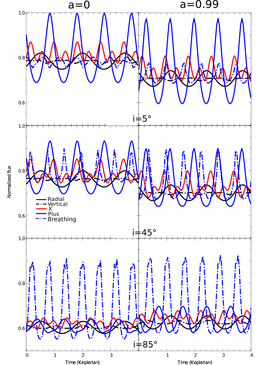
Figure 2: Light curves of a slender oscillating torus for spin $0$ (left column) or $0.99$ (right column) and inclination $5^{\circ}$ (upper row), $45^{\circ}$ (middle row) or $85^{\circ}$ (lower row). All five oscillation modes investigated in this article are represented on each panel (radial mode in solid black, vertical mode in dashed black, X mode in solid red, plus mode in solid blue and breathing mode in dashed blue). Times are in units of the Keplerian period at $r_{0}$ for spin $0$.

This Section shows the light curves and PSD of all five torus oscillation modes for two extreme values of spin, $a=0$ and $a=0.99$, and three values of inclinations $i=5^{\circ}$, $i=45^{\circ}$ and $i=85^{\circ}$. All other parameters are fixed to the values given in Tab. 3. Figs. 2 and 3 show respectively the light curves and PSD for all oscillation modes, spins and inclinations. Three effects are particularly important to explain the modulation of light curves and the corresponding amplitude of PSD:

• the general relativistic redshift effect that has an impact on the observed intensity: $I_{\nu}^{\mathrm{obs}}=g^{4}I_{\nu}^{\mathrm{em}}$ where $g=\nu^{\mathrm{em}}/\nu^{\mathrm{obs}}$ and $\nu^{\mathrm{em}}$ is related to the emitter’s 4-velocity,

• the time variation of the emitting area in the emitter’s frame $A_{\mathrm{em}}$, that is linked to the variation of the surface function, and the resulting change of emitted intensity (see Eq. 33),

• the time variation of the apparent torus area on the observer’s sky $A_{\mathrm{app}}$, that is a function of the variation of $A_{\mathrm{em}}$, of the bending of photons geodesics and of the inclination angle.

The vertical mode is relevant to determine the impact of the first effect. This mode has constant $A_{\mathrm{em}}$, and $A_{\mathrm{app}}$ is also barely varying for all inclinations. The light curve modulation is thus mainly due to the variation of the emitter’s 4-velocity. Given the extremely low level of modulation for this vertical mode, it appears that the effect of general relativistic redshift variation is negligible compared to the time variation of the emitting and the apparent torus areas.

The observed flux is essentially equal to the apparent area $A_{\mathrm{app}}$ of the torus multiplied by the observed intensity. Neglecting the redshift effect, the observed intensity varies due to the intrinsic variation of the emitted intensity which in turn is linked to the intrinsic variation of the emitted area $A_{\mathrm{em}}$. The total modulation depends on the respective weights of these effects.

4.3.1 Impact of inclination

The very strong dependence of the spectra on inclination shows that the most important effect is the variation of apparent area, which is the only inclination dependent effect. This can be quantified by comparing the variation of $A_{\mathrm{em}}$ and $A_{\mathrm{app}}$. Let us take the breathing mode at spin $0$ as an example. While the emitting area can vary up to $20\%$ during the course of the oscillation, the apparent area changes by $12\%$ for a face-on torus ($i=5^{\circ}$) and by $80\%$ for and edge-on torus ($i=85^{\circ}$), whereas the flux varies by $6\%$ at $5^{\circ}$ and $65\%$ at $85^{\circ}$, respectively. The variation of $A_{\mathrm{em}}$ (and subsequent inverse variation of emitted intensity) thus leads to somewhat restraining the effect of the variation of $A_{\mathrm{app}}$.

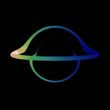
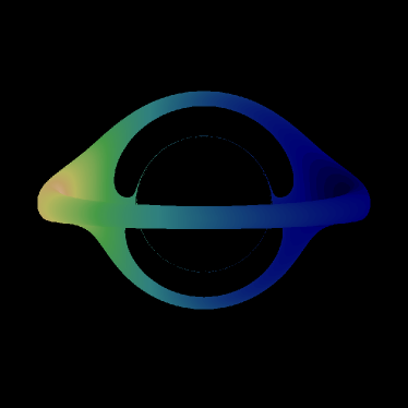
Figure 1: Breathing mode images at spin $0$ and inclination $85^{\circ}$. The two panels correspond to the two extreme values of the torus apparent area. The observed intensity of every pixel is reduced when the apparent size is bigger, as the emitted intensity decreases when the emitting area increases. Although it does not seem so from the torus apparent area variation, the torus remains slender at all times. These images are highly distorted by general relativistic effects.

Fig. 1 shows the two images of the breathing mode at $85^{\circ}$ of inclination corresponding to the extreme values of $A_{\mathrm{app}}$.

The plus and breathing modes are particularly sensitive to inclination. This is due to the fact that the torus cross-section is modified differently in the vertical and horizontal directions, where vertical refers to the direction orthogonal to the equatorial plane and horizontal inside the equatorial plane. The plus mode leads mainly to a horizontal motion whereas the breathing mode induces mainly a vertical movement. This ends up in the plus mode being more modulated at small inclinations as horizontal motions are more visible for a face-on observer. The opposite is true for the breathing mode.

The X mode is special in the sense that it is the only mode leading to a strong first harmonic whatever the inclination. This is due to the particular variation of the torus surface for this mode, that leads to two local maxima of apparent area $A_{\mathrm{app}}$ per Keplerian period. These two local maxima of $A_{\mathrm{app}}$ have different values, leading to different values of flux local maxima.

4.3.2 Impact of spin

The first difference due to the spin parameter is the value of the peak frequency, $\sigma_{i}$ (see Tab. 1), which is a function of spin. For instance, $\sigma_{+}$ varies from $1.03$ ($a=0$) to $1.2$ ($a=0.99$) in units of the Keplerian frequency. The breathing mode frequency varies less, going from $1.67$ ($a=0$) to $1.64$ ($a=0.99$). This spin-related difference of frequency is clearly visible in the upper and lower panels of Fig. 2.

Regarding the total power of the modulation, the most stringent difference is associated to the plus and breathing modes that always lead to a high-spin power greater or equal to the low-spin power. For instance, the plus mode at inclination $5^{\circ}$ has around $40\%$ more power at spin $0.99$ than at spin $0$. This increase in power with spin is dictated by the combined impact of the variation of emitting and apparent areas. Taking the plus mode as an example, its emitting area varies a bit less at higher spin while the apparent area at low inclination varies significantly more. These two effects lead to a higher modulation at higher spin.

Modes other than plus and breathing have comparable power at both spins due to the fact that the apparent area of the torus varies by a similar amount for the two spin values.

A third effect of the spin parameter is to change the relative values of the powers of different modes. For instance, the power ratio between the plus and breathing modes at inclination $5^{\circ}$ is of around $50$ at spin $0$ and $20$ at spin $0.99$. At inclination $85^{\circ}$ this ratio is evolving from $35$ to $10$. The dependence of this ratio with spin is mainly dictated by the evolution of the apparent area: the respective evolutions of $A_{\mathrm{app}}$ for the plus and breathing modes are more different at lower than at higher spin.

The conclusion of this analysis is that both inclination and spin have a clear impact on the power spectra. These parameters are key to determining the apparent area of the torus as a function of time, which itself dictates the modulation of the light curve. In particular, the plus and breathing modes are extremely sensitive to these two parameters:

• The peak frequency of their PSD is a function of spin;

• Plus mode has less power at higher inclination and breathing mode more power;

• Plus and breathing modes have more power at higher spins;

• The ratio of the breathing mode to plus mode powers is a function of spin and inclination.

These features may be used to constrain spin and inclination by fitting the theoretical spectra to observed QPO data. However, our model is still too simple to allow us putting this possibility to the test.

5 Conclusions and perspectives

This article is devoted to computing the spectral signature of the lowest order oscillation modes of slender accretion tori with constant angular momentum surrounding Kerr black holes.

We show how the ray-traced light curves and power spectral densities are regulated by the oscillation mode, the inclination and the spin parameter. The power of a given mode has a strong and non-linear dependence on spin and inclination. We find that both plus and breathing modes dominate the high spin regime at all inclinations. For low spin, either the plus or the breathing mode is dominating, with a strong dependence on the inclination parameter. Lower order modes are much less sensitive to changing the spin, but they still vary with the inclination. This may imply that depending on black hole spin and inclination of an X-ray binary system the observed high-frequency QPOs would be attributed to different oscillation modes. If true, then there would be no unique pair of modes that describes the observed 3:2 resonance in all black hole sources with QPOs. Rather, each black hole binary system would have its own characteristic mode combination which would be visible at its individual inclination and spin. However, we caution that our model is still too simple to draw any conclusions. How QPOs are excited and which oscillation modes are at work is at this point still unclear. Magneto-hydrodynamical simulations of radiation dominated accretion discs suggest on the one hand that the breathing mode is the strongest of the oscillation modes, but on the other hand that it is, like all higher order acoustic modes (but unlike the epicyclic modes), damped at a rate proportional to the disc scale height (see Blaes et al., 2011).

This work also highlights the importance of ray-tracing for computing power spectra of oscillating tori. Previous works have suggested that the 3:2 double peak may be due to a resonance between the radial and vertical modes (Abramowicz & Kluźniak, 2001), the radial and plus modes (Rezzolla et al., 2003) or the vertical and breathing modes (Blaes et al., 2006). The fact that the power exhibited by these modes is so different in our simulations (which is a consequence of ray-tracing, as the power is mainly linked with the variation of the torus apparent area) should be taken into account in these models.

A natural follow-up of this analysis will be to determine to what extent inclination and spin could be constrained by fitting this model to QPO data. In order to be able to answer this question, the oscillating torus model should be made more realistic. Future work will be devoted to developing general-relativistic magneto-hydrodynamics (GRMHD) simulations of non-equilibrium slender tori in order to determine which oscillation modes are the most likely to be triggered and with what strength.

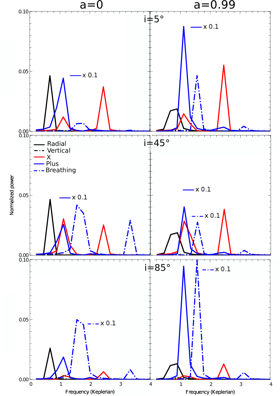
Figure 3: Power spectral density of a slender oscillating torus for spin $0$ (left column) or $0.99$ (right column) and inclination $5^{\circ}$ (upper row), $45^{\circ}$ (middle row) or $85^{\circ}$ (lower row). All five oscillation modes investigated in this article are represented on each panel (radial mode in solid black, vertical mode in dashed black – invisible because too weak, X mode in solid red, plus mode in solid blue and breathing mode in dashed blue). Note that some spectra are multiplied by $0.1$ for convenience. Frequencies are in units of the Keplerian frequency at $r_{0}$ for spin $0$.