Integral Reduction by Unitarity Method for Two-loop Amplitudes: A Case Study

Abstract:

In this paper, we generalize the unitarity method to two-loop diagrams and use it to discuss the integral bases of reduction. To test out method, we focus on the four-point double-box diagram as well as its related daughter diagrams, i.e., the double-triangle diagram and the triangle-box diagram. For later two kinds of diagrams, we have given complete analytical results in general $(4-2\epsilon)$-dimension.

1 Introduction

Currently, the focus of high energy physics is the LHC experiment. To understand the experiment data, we need to evaluate scattering amplitudes to high accuracy level required by data. Thus for most processes, the one-loop evaluation becomes necessary. In last ten years, enormous progress has been made in the computation of one-loop scattering amplitudes(see, for example, the references [1, 2, 3] and citations in the papers). However, for some processes in modern colliders, such as the process $gg\to\gamma\gamma$ which is an important background for searching the Higgs boson at the LHC, one-loop amplitudes do not suffice since their leading-order terms begin at one loop. Thus next-to-leading order corrections require the computation of two-loop amplitudes [4, 5, 6].

The traditional method for amplitude calculation is through the Feynman diagram. This method is well organized and has clear physical picture. It has also been implemented into many computer programs. However, with increasing of loop level or the number of external particles, the complexity of computation increases dramatically. Thus even with the most powerful computer available, many interesting processes related to LHC experiments can not be dealt by the traditional method.

To solve the challenge, many new methods(see books [7, 8, 9]) have been developed, such as IBP(integrate-by-part) method [10, 11, 12, 13, 14, 15, 16, 17, 18, 19](some new developments, see [20, 21, 22]), differential equation method [23, 24, 25, 26, 27, 28, 29, 30], MB(Mellin-Barnes) method [31, 32, 33, 34], etc. Among these methods, the reduction method [35, 36, 37, 38] is one of the most useful methods. More explicitly, the reduction of an amplitude means that any amplitude ${\cal A}$ can be expanded by bases(or ”master integral”) as

$${\cal A}=\sum_{i}c_{i}{\cal A}_{i}~{},~{}~{}~{}$$ (1)

with rational coefficients $c_{i}$. With this expansion, the amplitude calculation can be separated into two parts: (a) the evaluation of bases(or master integrals) at given loop order and (b) the determination of coefficients $c_{i}$ for a particular process. For the former part, it can be done once for all and the results can be applied to any process. Thus in the practical application, the latter part, i.e., the determination of coefficients, becomes the central focus of all calculations.

Unitarity method is an ideal tool to determine coefficients[39, 40, 41, 42, 43, 44, 45, 46, 47, 48, 49, 50, 51, 52, 53, 54]. With the expansion (1), if we perform unitarity cut on both sides, we will get

$$\Delta{\cal A}=\sum_{i}c_{i}\Delta{\cal A}_{i}~{}.~{}~{}~{}$$ (2)

So if both $\Delta{\cal A}$ and $\Delta{\cal A}_{i}$ can be evaluated analytically, and if different $\Delta{\cal A}_{i}$ has distinguishable analytic structure(which we will call the ”signature” of basis under the unitarity cut), we can compare both sides of (2) to determine coefficients $c_{i}$, analogous to the fact that if two polynomials of $x$ are equal, so are their coefficients of each term $x^{n}$. The unitarity method has been proven to be very successful in determining coefficients for one-loop amplitudes(see reviews [55, 56]). For some subsets of bases(such as box topology for one-loop and double-box topology for planar two-loop), more efficient method, the so called ”generalized unitarity method”(or ”maximum unitarity cut” or ”leading singularity”), has been developed [43, 57, 58, 59, 60, 61, 62, 63, 64, 65, 66, 67].

The applicability of reduction method is based on the valid expression of expansion (1). Thus the determination of bases becomes the first issue. From recent study, it is realized that there are two kinds of bases: the integrand bases and the integral bases. The integrand bases are algebraically independent rational functions before performing loop integration. For one-loop, the integrand bases have been determined by OPP[68]. For two-loop or more, the computational algebraic geometry method has been proposed to determine the integrand bases [69, 70, 71, 72, 73, 74, 75, 76, 77, 78, 79].

In general the number of integrand bases is larger than the number of integral bases, because after loop integration, some combinations of integrand bases may vanish. For one-loop amplitudes, the difference between these two numbers is not very significant. For example, the number of integral bases is one while the number of integrand bases is seven for triangle topology of renormalizable field theories[68]. However, for two-loop amplitudes, the difference could be huge. As we will show later, for double-triangle topology, there are only several integral bases, while the number of integrand bases is about one hundred for renormalizable field theories[78]. Thus the determination of integral bases for two-loop and higher-loop becomes necessary.

Although integrand bases can be determined systematically, the determination of integral bases is far from being completely solved. It is our attempt in this paper to find an efficient method to solve the problem. Noticing that in the unitarity method, the action $\Delta$ in (2) is directly acting on the integrated results, thus if the left hand side $\Delta{\cal A}$ can be analytically integrated for arbitrary inputs, we can classify independent distinguishable analytic structures from these results. Each structure should correspond to one integral basis. By this attempt we can determine integral bases.

In this paper, taking double-box topology and its daughter topologies as examples, we generalize unitarity method to two-loop amplitudes and try to determine the integral bases. Different from the maximal unitarity method[60], we cut only four propagators(the propagator with mixed loop momenta will not be touched). Comparing with maximal unitarity cut where solutions for loop momenta are complex number in general, our cut conditions guarantee the existence of real solutions for loop momenta, thus avoiding the affects from spurious integrations.

This paper is organized as follows. In section 2 we review the one-loop unitarity method and then generalize the scheme to two-loop. For two-loop, two sub-one-loop phase space integrations should be evaluated. In section 3, we integrate the first sub-one-loop integration of triangle topology. The result is used in section 4, where integration over the second sub-one-loop of triangle topology is performed. Results obtained in this section allow us to determine integral bases for the topology ${\cal A}_{212}$. Results in section 3 is also also used in section 5, where integration over the second sub-one-loop of box topology is performed, and the result can be used to determine integral bases for topology ${\cal A}_{213}$. In section 6, we briefly discuss the integral bases of topology ${\cal A}_{313}$ since results are well known for this topology. Finally, in section 7, a short conclusion is given.

Technical details of calculation are presented in Appendix. In Appendix A, some useful formulae for phase space integration are summarized. In Appendix B, the phase space integration is done for one-loop bubble, one-loop triangle and one-loop box topologies. In Appendix C, details of an integration for topology ${\cal A}_{313}$ are discussed.

2 Setup

In this section, we present some general discussions about the calculation done in this paper. Firstly, we review how to do the phase space integration in unitarity method illustrated by one-loop example. Then we set up the framework in unitarity method for two-loop topologies which are the starting point of this paper.

2.1 Phase space integration

The unitarity method has been successfully applied to one-loop amplitudes [39, 40, 41, 42, 43, 44, 45, 46, 47, 48, 49, 50, 51, 52, 53, 54] . Here we give a brief summary about the general $(4-2\epsilon)$-dimensional unitarity method[51, 52], which will be used later. Through this paper we use the metric $\eta_{\mu\nu}=(+,-,...,-)$ and QCD convention for spinors, i.e., $2k_{i}\cdot k_{j}\equiv\left\langle k_{i}|k_{j}\right\rangle\left[k_{j}|k_{i}\right]$.

For one-loop, the action $\Delta$ in (2) is realized by putting two internal propagators on-shell. More explicitly, let us consider the following most general input with massless internal propagators

$${\cal A}^{(a)}_{n} \equiv \int d^{4-2\epsilon}\widehat{\ell}{\cal I}_{n}^{(a)}=\int d^{4-2\epsilon}\widehat{\ell}{(2\widehat{\ell}\cdot T)^{a}\over\widehat{\ell}^{2}\prod_{i=1}^{n-1}(\widehat{\ell}-K_{i})^{2}}~{},~{}~{}~{}$$ (3)

where the inner momentum is in $(4-2\epsilon)$-dimensional space and all external momenta are in pure 4D space for our regularization scheme. The unitarity cut with intermediate flowing momentum $K$ is given by putting $\widehat{\ell}^{2}$ and $(\widehat{\ell}-K)^{2}$ on-shell, and we get the expression

$$\Delta{\cal A}^{(a)}_{n}=\int d^{4-2\epsilon}\widehat{\ell}{(2\widehat{\ell}\cdot T)^{a}\delta(\widehat{\ell}^{2})\delta((\widehat{\ell}-K)^{2})\over\prod_{i=1}^{n-2}(\widehat{\ell}-K_{i})^{2}}~{}.~{}~{}~{}$$ (4)

With two delta-functions, the original $(4-2\epsilon)$-dimensional integration is reduced to $(2-2\epsilon)$-dimensional integration. To carry out the remaining integration, we decompose $\widehat{\ell}$ as $\widehat{\ell}=\widetilde{\ell}+\mu$, where $\widetilde{\ell}$ is the pure 4D part while $\mu$ is the $(-2\epsilon)$-dimensional part[51], then the measure becomes

$$\int d^{4-2\epsilon}\widehat{\ell}\delta(\widehat{\ell}^{2})\delta((\widehat{\ell}-K)^{2})(\bullet)=\int d^{-2\epsilon}\mu\int d^{4}\widetilde{\ell}\delta(\widetilde{\ell}^{2}-\mu^{2})\delta((\widetilde{\ell}-K)^{2}-\mu^{2})(\bullet)~{}.~{}~{}~{}$$ (5)

Next, we split $\widetilde{\ell}$ into $\widetilde{\ell}=\ell+zK$ with $\ell^{2}=0$ to arrive

$$\int d^{4}\widetilde{\ell}\delta(\widetilde{\ell}^{2}-\mu^{2})\delta((\widetilde{\ell}-K)^{2}-\mu^{2})(\bullet)$$ (6)

$$= \int dzd^{4}\ell\delta(\ell^{2})(2\ell\cdot K)\delta(z^{2}K^{2}+2z\ell\cdot K-\mu^{2})\delta((1-2z)K^{2}-2\ell\cdot K)(\bullet)~{}.~{}~{}~{}$$

Having the form (6), we can use the following well known result of spinor integration[80]. Define null momentum as $\ell=t\lambda\widetilde{\lambda}$, then

$$\int d^{4}\ell\delta^{+}(\ell^{2})(\bullet)=\int_{0}^{+\infty}tdt\int\left\langle\lambda|d\lambda\right\rangle\left[\widetilde{\lambda}|d\widetilde{\lambda}\right](\bullet)~{}.~{}~{}~{}$$ (7)

Substituting (7) back to (6), we can use remaining two delta-functions to fix $t$ and $z$ as

$$z={1-\sqrt{1-u}\over 2}~{}~{},~{}~{}t={(1-2z)K^{2}\over\left\langle\lambda|K|\widetilde{\lambda}\right]}~{}~{},~{}~{}u\equiv{4\mu^{2}\over K^{2}}~{}.~{}~{}~{}$$ (8)

After above simplification, the integral (4) is transformed to the following spinor form

$$\Delta{\cal A}^{(a)}_{n} = \int d^{-2\epsilon}\mu\int\left\langle\lambda|d\lambda\right\rangle\left[\widetilde{\lambda}|d\widetilde{\lambda}\right]{(-)^{n-2}[(1-2z)K^{2}]^{a-n+3}\left\langle\lambda|R|\widetilde{\lambda}\right]^{a}\over\left\langle\lambda|K|\widetilde{\lambda}\right]^{a-n+4}\prod_{i=1}^{n-2}\left\langle\lambda|Q_{i}|\widetilde{\lambda}\right]}~{},~{}~{}~{}$$ (9)

where

$$R\equiv T+{z(2K\cdot T)\over(1-2z)K^{2}}K~{}~{},~{}~{}Q_{i}\equiv K_{i}+{z(2K\cdot K_{i})-K_{i}^{2}\over(1-2z)K^{2}}K~{}.~{}~{}~{}$$ (10)

To deal with the integral like $\int\left\langle\lambda|d\lambda\right\rangle\left[\widetilde{\lambda}|d\widetilde{\lambda}\right]f(\lambda,\widetilde{\lambda})$ when $f(\lambda,\widetilde{\lambda})$ is a rational function, the first step is to find a function $g(\lambda,\widetilde{\lambda})$ satisfying

$$\int\left\langle\lambda|d\lambda\right\rangle\left[\widetilde{\lambda}|d\widetilde{\lambda}\right]f(\lambda,\widetilde{\lambda})=\int\left\langle\lambda|d\lambda\right\rangle\left[d\widetilde{\lambda}|{\partial\over\partial\widetilde{\lambda}}\right]g(\lambda,\widetilde{\lambda})~{}.~{}~{}~{}$$ (11)

With $g(\lambda,\widetilde{\lambda})$, the integration is given algebraically by the sum of residues of holomorphic pole in $g(\lambda,\widetilde{\lambda})$[46]. In Appendix B, we summarize some general results of standard one-loop integrations using above technique. It is worth to mention that for two-loop, $f(\lambda,\widetilde{\lambda})$ might not be rational function. We will discuss how to deal with it later.

We also want to remark that under the framework of $(4-2\epsilon)$-dimensional unitarity method, coefficient of each basis will be polynomial of $\mu^{2}$(remembering the splitting $\widehat{\ell}=\widetilde{\ell}+\mu$). There are two ways to handle it. For the first way, one can further integrate $\int d^{-2\epsilon}\mu~{}(\mu^{2})^{n}$ to find coefficients depending on $\epsilon$. For the second way, we just keep $\mu^{2}$, but include the dimensional shifted scalar basis[42, 81], such as

$${\cal A}^{D=(4-2\epsilon)}[(\mu^{2})^{r}]\equiv\int d^{-2\epsilon}\mu d^{4}\widetilde{\ell}{(\mu^{2})^{r}\over(\widetilde{\ell}^{2}-\mu^{2})\prod_{i=1}^{n-1}((\ell-K_{i})^{2}-\mu^{2})}~{}.~{}~{}~{}$$ (12)

This is equivalent to

$${\cal A}^{D=(4-2\epsilon)}[(\mu^{2})^{r}]=-\epsilon(1-\epsilon)...(r-1-\epsilon){\cal A}^{D=(4+2r-2\epsilon)}[1]~{}.~{}~{}~{}$$ (13)

For one-loop, dimensional shifted bases are often used. In this paper we adapt the similar strategy, i.e., keeping the $\mu$-part and introducing the dimensional shifted bases.

2.2 Generalizing to two-loop case

In this subsection, we set up unitarity method for two-loop amplitudes, particularly for the attempt of determining integral bases.

The first problem is to decide which propagators should be cut. There are three kinds of propagators: (1) propagators depending on $\widehat{\ell}_{1}$ only; (2) propagators depending on $\widehat{\ell}_{2}$ only; (3) propagators depending on both $\widehat{\ell}_{1}$ and $\widehat{\ell}_{2}$. In principle, we can cut any propagators, but for simplicity, in this paper we will cut propagators of the first two kinds. For our choice, we cut two propagators of the first kind and two propagators of the second kind. With this arrangement, for each loop it is exactly the familiar unitarity method in one-loop case.

Next we set up notation for two-loop integral. The two internal momenta are denoted as $\widehat{\ell}_{1},\widehat{\ell}_{2}$ in $(4-2\epsilon)$-dimension, while all external momenta are in pure 4-dimension. We use $n_{1},n_{2},n_{12}$ to denote the number of each kind of propagators respectively. Then a general integrand with massless propagators can be represented by

$${\cal I}_{n_{1}n_{12}n_{2}}^{(a,b)}\equiv{(2\widehat{\ell}_{1}\cdot T_{1})^{a}(2\widehat{\ell}_{2}\cdot T_{2})^{b}\over[\widehat{\ell}_{1}^{2}\prod_{i=1}^{n_{1}-1}(\widehat{\ell}_{1}-K_{1i})^{2}][\widehat{\ell}_{2}^{2}\prod_{j=1}^{n_{2}-1}(\widehat{\ell}_{2}-K_{2j})^{2}][(\widehat{\ell}_{1}+\widehat{\ell}_{2})^{2}\prod_{t=1}^{n_{12}-1}(\widehat{\ell}_{1}+\widehat{\ell}_{2}-K_{t})^{2}]}~{}.~{}~{}~{}$$ (14)

The unitarity cut action $\Delta$ is then given by

$$\Delta{\cal A} = \int\prod_{i=1}^{2}d^{4-2\epsilon}\widehat{\ell}_{i}\left\{{\cal I}_{n_{1}n_{12}n_{2}}^{(a,b)}\prod_{i=1}^{2}\widehat{\ell}_{i}^{2}(\widehat{\ell}_{i}-K_{L_{i}})^{2}\right\}\prod_{i=1}^{2}\delta(\widehat{\ell}_{i}^{2})\delta((\widehat{\ell}_{i}-K_{L_{i}})^{2})~{}.~{}~{}~{}$$ (15)

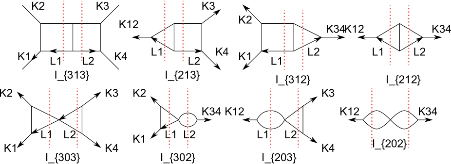
Figure 1: The unitarity cut of double box topology $I_{313}$ as well as its seven daughter topologies. The dashed red lines indicate cuts.

With above setup, we take a well studied example[20, 60, 61, 62, 63, 64, 65, 66], i.e., the four-point two-loop double-box(${\cal A}_{313}$) integral as the target to apply the unitarity method and determine integral bases. The integrand is given by

$${\cal I}^{(a,b)}_{313} = {(2\widehat{\ell}_{1}\cdot T_{1})^{a}(2\widehat{\ell}_{2}\cdot T_{2})^{b}\over\widehat{\ell}_{1}^{2}(\widehat{\ell}_{1}-K_{1})^{2}(\widehat{\ell}_{1}-K_{12})^{2}\widehat{\ell}_{2}^{2}(\widehat{\ell}_{2}-K_{4})^{2}(\widehat{\ell}_{2}-K_{34})^{2}(\widehat{\ell}_{1}+\widehat{\ell}_{2})^{2}}~{},~{}~{}~{}$$ (16)

and the four propagators to be cut are

$$\widehat{\ell}_{1}^{2}~{}~{},~{}~{}(\widehat{\ell}_{1}-K_{12})^{2}~{}~{},~{}~{}\widehat{\ell}_{2}^{2}~{}~{},~{}~{}(\widehat{\ell}_{2}-K_{34})^{2}~{},~{}~{}~{}$$

where $K_{12}+K_{34}=0$. With this choice of cuts, in order to completely understand the results, we also need to consider other topologies besides double-box. The other contributions come from those topologies by pinching one or more un-cut propagators of double-box, as shown in Figure 1. There are three daughter topologies ${\cal I}_{213},{\cal I}_{312},{\cal I}_{303}$ by pinching one propagator. There are also three daughter topologies ${\cal I}_{212},{\cal I}_{302},{\cal I}_{203}$ by pinching two propagators. Finally there is only one daughter topology ${\cal I}_{202}$ by pinching three propagators. Among them, ${\cal I}_{303},{\cal I}_{203},{\cal I}_{302},{\cal I}_{202}$ are direct products of two one-loop topologies, thus their signatures are well known(see Appendix B). So in fact we need to examine two non-trivial topologies ${\cal I}_{212},{\cal I}_{213}$(by symmetry ${\cal I}_{312}$ is equivalent to ${\cal I}_{213}$) together with the mother topology ${\cal I}_{313}$. Integrand of these two additional topologies are given by

$${\cal I}^{(a,b)}_{212} = {(2\widehat{\ell}_{1}\cdot T_{1})^{a}(2\widehat{\ell}_{2}\cdot T_{2})^{b}\over\widehat{\ell}_{1}^{2}(\widehat{\ell}_{1}-K_{12})^{2}\widehat{\ell}_{2}^{2}(\widehat{\ell}_{2}-K_{34})^{2}(\widehat{\ell}_{1}+\widehat{\ell}_{2})^{2}}~{},~{}~{}~{}$$

$${\cal I}^{(a,b)}_{213} = {(2\widehat{\ell}_{1}\cdot T_{1})^{a}(2\widehat{\ell}_{2}\cdot T_{2})^{b}\over\widehat{\ell}_{1}^{2}(\widehat{\ell}_{1}-K_{12})^{2}\widehat{\ell}_{2}^{2}(\widehat{\ell}_{2}-K_{4})^{2}(\widehat{\ell}_{2}-K_{34})^{2}(\widehat{\ell}_{1}+\widehat{\ell}_{2})^{2}}~{}.~{}~{}~{}$$ (17)

In the following sections, we will study ${\cal I}_{212}$, ${\cal I}_{213}$ and ${\cal I}_{313}$ one by one, and our basic strategy will be to integrate one loop momentum $\widetilde{\ell}_{1}$ first while keeping $\widetilde{\ell}_{2}$ arbitrarily. Then we analyze the integration of $\widetilde{\ell}_{2}$ based on the previous results.

3 The $\widetilde{\ell}_{1}$-part integration ($n_{1}=2$)

In this section, we do the $\widetilde{\ell}_{1}$ integration. Using the standard method for one-loop amplitudes(reviewed in previous section as well as in Appendix B) we get(see formula (14))

$$\Delta{\cal A}_{n_{1}1n_{2}}^{(a,b)} = \int d^{-2\epsilon}\mu_{1}d^{-2\epsilon}\mu_{2}d^{4}\widetilde{\ell}_{2}\delta(\widetilde{\ell}_{2}^{2}-\mu_{2}^{2})\delta(K_{L_{2}}^{2}-2K_{L_{2}}\cdot\widetilde{\ell}_{2}){(2\widetilde{\ell}_{2}\cdot T_{2})^{b}\over\prod_{j=1}^{n_{2}-2}((\widetilde{\ell}_{2}-K_{2j})^{2}-\mu_{2}^{2})}$$ (18)

$$\int\left\langle\lambda_{1}|d\lambda_{1}\right\rangle\left[\widetilde{\lambda}_{1}|d\widetilde{\lambda}_{1}\right]{(-)^{n_{1}-2}((1-2z_{1})K_{L_{1}}^{2})^{a-n_{1}+2}\over\left\langle\lambda_{1}|K_{L_{1}}|\widetilde{\lambda}_{1}\right]^{a-n_{1}+3}}{\left\langle\lambda_{1}|R_{1}|\widetilde{\lambda}_{1}\right]^{a}\over\left\langle\lambda_{1}|W_{1}|\widetilde{\lambda}_{1}\right]\prod_{i=1}^{n_{1}-2}\left\langle\lambda_{1}|Q_{1i}|\widetilde{\lambda}_{1}\right]}~{},~{}~{}~{}$$

where various quantities are defined as

$$R_{1} \equiv T_{1}+{z_{1}2K_{L_{1}}\cdot T_{1}\over(1-2z_{1})K_{L_{1}}^{2}}K_{L_{1}}~{},~{}~{}~{}$$

$$Q_{1i} \equiv K_{1i}+{z_{1}(2K_{L_{1}}\cdot K_{1i})-K_{1i}^{2}\over(1-2z_{1})K_{L_{1}}^{2}}K_{L_{1}}~{},~{}~{}~{}$$

$$W_{1} \equiv \widetilde{\ell}_{2}+{(\widetilde{\ell}_{2}^{2}-\mu_{2}^{2})-2\mu_{1}\cdot\mu_{2}+2z_{1}\widetilde{\ell}_{2}\cdot K_{L_{1}}\over(1-2z_{1})K_{L_{1}}^{2}}K_{L_{1}}~{},~{}~{}~{}$$ (19)

with $z_{1}={1-\sqrt{1-u_{1}}\over 2}$ and $u_{1}={4\mu_{1}^{2}\over K_{L_{1}}^{2}}$. Note that here the left cut momentum $K_{L_{1}}=K_{12}$ is the same to the right cut momentum $K_{L_{2}}=K_{34}$ up to a sign, however we keep them independently so that it is possible to formulate them to more general situations. The $W_{1}$ comes from the mixed propagator $(\widehat{\ell}_{1}+\widehat{\ell}_{2})^{2}$. Situations with non trivial topologies ${\cal A}_{313}$, ${\cal A}_{312}$, ${\cal A}_{213}$ and ${\cal A}_{212}$ are all included in the formula (18).

Let us apply our general framework to the specific case $n_{1}=2$. The general formula (18) now becomes

$$\Delta{\cal A}_{n_{1}1n_{2}}^{(a,b)}\Big{|}_{n_{1}=2} = \int d^{-2\epsilon}\mu_{1}d^{-2\epsilon}\mu_{2}d^{4}\widetilde{\ell}_{2}\delta(\widetilde{\ell}_{2}^{2}-\mu_{2}^{2})\delta(K_{L_{2}}^{2}-2K_{L_{2}}\cdot\widetilde{\ell}_{2}){(2\widetilde{\ell}_{2}\cdot T_{2})^{b}\over\prod_{j=1}^{n_{2}-2}((\widetilde{\ell}_{2}-K_{2j})^{2}-\mu_{2}^{2})}$$ (20)

$$\int\left\langle\lambda_{1}|d\lambda_{1}\right\rangle\left[\widetilde{\lambda}_{1}|d\widetilde{\lambda}_{1}\right]{((1-2z_{1})K_{L_{1}}^{2})^{a}\over\left\langle\lambda_{1}|K_{L_{1}}|\widetilde{\lambda}_{1}\right]^{a+1}}{\left\langle\lambda_{1}|R_{1}|\widetilde{\lambda}_{1}\right]^{a}\over\left\langle\lambda_{1}|W_{1}|\widetilde{\lambda}_{1}\right]}~{}.~{}~{}~{}$$

The second line is nothing but the standard one-loop triangle integration(see Appendix B). When $a=0$, the integration gives the signature of triangle part. When $a\geq 1$, the integration can be decomposed into both triangle part and bubble part. We will evaluate contributions from these two parts separately.

3.1 The contribution to triangle part

The triangle signature : Based on our general formula of the standard one-loop triangle integration (117), the signature of the triangle part is

$${\cal S}_{tri}\equiv{1\over\sqrt{\Delta_{W_{1},K_{L_{1}}}}}\ln\left({W_{1}\cdot K_{L_{1}}-\sqrt{(W_{1}\cdot K_{L_{1}})^{2}-W_{1}^{2}K_{L_{1}}^{2}}\over W_{1}\cdot K_{L_{1}}+\sqrt{(W_{1}\cdot K_{L_{1}})^{2}-W_{1}^{2}K_{L_{1}}^{2}}}\right)~{}.~{}~{}~{}$$ (21)

Imposing cut conditions for $\widetilde{\ell}_{2}$, i.e., $\delta(\widetilde{\ell}_{2}^{2}-\mu_{2}^{2})$ and $\delta(K_{L_{2}}^{2}-2K_{L_{2}}\cdot\widetilde{\ell}_{2})$ we can simplify it to

$${\cal S}_{tri} = {1\over K_{L_{1}}^{2}\sqrt{1-u_{2}}}\ln\left({(4\mu_{1}\cdot\mu_{2}+K_{L_{1}}^{2})+\sqrt{(1-u_{1})(1-u_{2})}K_{L_{1}}^{2}\over(4\mu_{1}\cdot\mu_{2}+K_{L_{1}}^{2})-\sqrt{(1-u_{1})(1-u_{2})}K_{L_{1}}^{2}}\right)={1\over t_{2}K_{L_{1}}^{2}}\ln\Big{(}{s+t_{1}t_{2}\over s-t_{1}t_{2}}\Big{)}~{},~{}~{}~{}$$ (22)

where we have introduced

$$s={4\mu_{1}\cdot\mu_{2}+K_{L_{1}}^{2}\over K_{L_{1}}^{2}}~{}~{},~{}~{}t_{i}=\sqrt{1-u_{i}}~{}~{},~{}~{}u_{i}={4\mu_{i}^{2}\over K_{L_{i}}^{2}}~{}~{},~{}~{}i=1,2~{}.~{}~{}~{}$$ (23)

One can observe that the signature part does not depend on $\widetilde{\ell}_{2}$. It is an important feature which makes $\Delta{\cal A}_{21n_{2}}^{(a,b)}$ easier to be treated.

The coefficient ${\cal C}_{3\to 3}^{(a)}$: Using (117) the expression is

$${\cal C}_{3\to 3}^{(a)} = {(-)^{a}\over a!\Delta_{W_{1},K_{L_{1}}}^{a}}{d^{a}\over d\tau^{a}}\Big{(}\tau^{2}W_{1}^{2}+\tau(4W_{1}^{2}(R_{1}\cdot K_{L_{1}})-4(R_{1}\cdot W_{1})(W_{1}\cdot K_{L_{1}}))+R_{1}^{2}\Delta_{W_{1},K_{L_{1}}}$$ (24)

$$+(2R_{1}\cdot W_{1})^{2}K_{L_{1}}^{2}+(2R_{1}\cdot K_{L_{1}})^{2}W_{1}^{2}-(2R_{1}\cdot W_{1})(2R_{1}\cdot K_{L_{1}})(2W_{1}\cdot K_{L_{1}})\Big{)}^{a}\Big{|}_{\tau\to 0}~{}.~{}~{}~{}$$

Again, using cut conditions $\delta(\widetilde{\ell}_{2}^{2}-\mu_{2}^{2})$ and $\delta(K_{L_{2}}^{2}-2K_{L_{2}}\cdot\widetilde{\ell}_{2})$ we can do the following replacement

$$\widetilde{\ell}_{2}\to{(1-2z_{2})K_{L_{2}}^{2}\over\left\langle\lambda_{2}|K_{L_{2}}|\widetilde{\lambda}_{2}\right]}\lambda_{2}\widetilde{\lambda}_{2}+z_{2}K_{L_{2}}={(1-2z_{2})K_{L_{1}}^{2}\over-\left\langle\lambda_{2}|K_{L_{1}}|\widetilde{\lambda}_{2}\right]}\lambda_{2}\widetilde{\lambda}_{2}-z_{2}K_{L_{1}}~{},~{}~{}~{}$$

where $z_{2}={1-t_{2}\over 2}$. Since all derivatives act on $\tau$ only, such replacement will not affect the result. Some algebraic manipulations shows that the coefficients of different parts are given by

$$\tau^{2} : ~{}~{}{(s^{2}-t_{1}^{2}t_{2}^{2})K_{L_{1}}^{2}\over 4t_{1}^{2}}~{},~{}~{}~{}$$

$$\tau : {-t_{2}K_{L_{1}}^{2}\over t_{1}\left\langle\lambda_{2}|K_{L_{1}}|\widetilde{\lambda}_{2}\right]}\Big{(}t_{2}(K_{L_{1}}\cdot T_{1})\left\langle\lambda_{2}|K_{L_{1}}|\widetilde{\lambda}_{2}\right]+s(-(K_{L_{1}}\cdot T_{1})\left\langle\lambda_{2}|K_{L_{1}}|\widetilde{\lambda}_{2}\right]+K_{L_{1}}^{2}\left\langle\lambda_{2}|T_{1}|\widetilde{\lambda}_{2}\right])\Big{)}~{},~{}~{}~{}$$

$$\tau^{0} : {t_{2}^{2}(K_{L_{1}}^{2})^{2}\over\left\langle\lambda_{2}|K_{L_{1}}|\widetilde{\lambda}_{2}\right]^{2}}K_{L_{1}}^{2}\left\langle\lambda_{2}|(T_{1}+y_{1}K_{L_{1}})|\widetilde{\lambda}_{2}\right]\left\langle\lambda_{2}|(T_{1}+y_{2}K_{L_{1}})|\widetilde{\lambda}_{2}\right]~{},~{}~{}~{}$$ (25)

with

$$y_{1,2}={-(2T_{1}\cdot K_{L_{1}})\pm\sqrt{(2T_{1}\cdot K_{L_{1}})^{2}-4K_{L_{1}}^{2}T_{1}^{2}}\over 2K_{L_{1}}^{2}}~{}.~{}~{}~{}$$ (26)

To get non-zero contribution from ${d^{a}\over d\tau^{a}}(\bullet)\Big{|}_{\tau\to 0}$, we only need to take terms with $\tau^{a}$ power. It means that terms with $\tau^{2}$ in (25) will always appear with terms $\tau^{0}$, therefore we can regroup

$$\left\{\tau^{2}{(s^{2}-t_{1}^{2}t_{2}^{2})K_{L_{1}}^{2}\over 4t_{1}^{2}}\right\}+\left\{{t_{2}^{2}(K_{L_{1}}^{2})^{2}\over\left\langle\lambda_{2}|K_{L_{1}}|\widetilde{\lambda}_{2}\right]^{2}}K_{L_{1}}^{2}\left\langle\lambda_{2}|(T_{1}+y_{1}K_{L_{1}})|\widetilde{\lambda}_{2}\right]\left\langle\lambda_{2}|(T_{1}+y_{2}K_{L_{1}})|\widetilde{\lambda}_{2}\right]\right\}$$

to

$$\left\{\tau^{2}{t_{2}(s-t_{1}t_{2})(K_{L_{1}}^{2})^{2}\over 2t_{1}}{\left\langle\lambda_{2}|(T_{1}+y_{1}K_{L_{1}})|\widetilde{\lambda}_{2}\right]\over\left\langle\lambda_{2}|K_{L_{1}}|\widetilde{\lambda}_{2}\right]}\right\}+\left\{{t_{2}(s+t_{1}t_{2})(K_{L_{1}}^{2})^{2}\over 2t_{1}}{\left\langle\lambda_{2}|(T_{1}+y_{2}K_{L_{1}})|\widetilde{\lambda}_{2}\right]\over\left\langle\lambda_{2}|K_{L_{1}}|\widetilde{\lambda}_{2}\right]}\right\}~{}.~{}~{}~{}$$

Thus we can write

$${\cal C}_{3\to 3}^{(a)} = {(-)^{a}(K_{L_{1}}^{2})^{a}\over a!(t_{1}t_{2}K_{L_{1}}^{2})^{a}}{d^{a}\over d\tau^{a}}{\left\langle\lambda_{2}|{\cal F}|\widetilde{\lambda}_{2}\right]^{a}\over\left\langle\lambda_{2}|K_{L_{1}}|\widetilde{\lambda}_{2}\right]^{a}}\Big{|}_{\tau\to 0}~{},~{}~{}~{}$$

where ${\cal F}$ is defined as

$${\cal F} = -\tau\left(t_{2}{K_{L_{1}}\cdot T_{1}\over K_{L_{1}}^{2}}K_{L_{1}}+s\Big{(}T_{1}-{(K_{L_{1}}\cdot T_{1})\over K_{L_{1}}^{2}}K_{L_{1}}\Big{)}\right)$$ (27)

$$+\tau^{2}{s-t_{1}t_{2}\over 2}\Big{(}T_{1}+y_{1}K_{L_{1}}\Big{)}+{s+t_{1}t_{2}\over 2}\Big{(}T_{1}+y_{2}K_{L_{1}}\Big{)}~{}.~{}~{}~{}$$

Putting all results together, the triangle part becomes

$${\cal R}_{3\to 3}^{(a)} = \left({(-)^{a}(K_{L_{1}}^{2})^{a}\over a!(t_{1}t_{2}K_{L_{1}}^{2})^{a}}{d^{a}\over d\tau^{a}}{\left\langle\lambda_{2}|{\cal F}|\widetilde{\lambda}_{2}\right]^{a}\over\left\langle\lambda_{2}|K_{L_{1}}|\widetilde{\lambda}_{2}\right]^{a}}\Big{|}_{\tau\to 0}\right){1\over t_{2}K_{L_{1}}^{2}}\ln\Big{(}{s+t_{1}t_{2}\over s-t_{1}t_{2}}\Big{)}~{}.~{}~{}~{}$$ (28)

To do the $\widetilde{\ell}_{2}$-part integration, it is more convenient to use above form before taking the derivative over $\tau$.

3.2 The contribution to bubble part

Again we use results given in Appendix B.

The ${\cal R}_{3\to 2}[i,m]$ term: Using (119), the typical term of triangle topology to bubble is

$${\cal R}_{3\to 2}[i,m] = {(-)^{m+i}(K_{L_{1}}^{2})^{i}\over i!(m+1)\sqrt{\Delta(W_{1},K_{L_{1}})}^{m+2i+2}}{d^{i}\over d\tau^{i}}\left\{\left((2R_{1}\cdot P_{2}-\tau\left\langle P_{1}|R_{1}|P_{2}\right])^{m+1}\right.\right.$$ (29)

$$\left.(-x_{2}\left\langle P_{2}|R_{1}|P_{1}\right]-x_{1}\tau^{2}\left\langle P_{1}|R_{1}|P_{2}\right]+\tau(x_{2}(2R_{1}\cdot P_{1})+x_{1}(2R_{1}\cdot P_{2})))^{i}\right)$$

$$+(-)^{m}\left((2R_{1}\cdot P_{1}-\tau\left\langle P_{2}|R_{1}|P_{1}\right])^{m+1}\right.$$

$$\left.\left.(-x_{2}\tau^{2}\left\langle P_{2}|R_{1}|P_{1}\right]-x_{1}\left\langle P_{1}|R_{1}|P_{2}\right]+\tau(x_{2}(2R_{1}\cdot P_{1})+x_{1}(2R_{1}\cdot P_{2})))^{i}\right)\right\}\Big{|}_{\tau\to 0}~{},~{}~{}~{}$$

where two null momenta $P_{1},~{}P_{2}$ are constructed as $P_{i}=W_{1}+x_{i}K_{L_{1}}$, with

$$x_{1}={s+t_{1}t_{2}\over 2t_{1}}~{}~{},~{}~{}x_{2}={s-t_{1}t_{2}\over 2t_{2}}~{}.~{}~{}~{}$$

Again, to get non-zero contribution, $\left\langle P_{1}|R_{1}|P_{2}\right]$ and $\left\langle P_{2}|R_{1}|P_{1}\right]$ should always appear in pair. With a little calculations, one can see

$$\left\langle P_{1}|R_{1}|P_{2}\right]\left\langle P_{2}|R_{1}|P_{1}\right]={\cal T}_{1}{\cal T}_{2}~{}~{},~{}~{}{\cal T}_{i}=\left({t_{2}K_{L_{1}}^{2}\over\left\langle\lambda_{2}|K_{L_{1}}|\widetilde{\lambda}_{2}\right]}\right)\left\langle\lambda_{2}|(T_{1}+y_{i}K_{L_{1}})|\widetilde{\lambda}_{2}\right]~{},~{}~{}~{}$$ (30)

where $y_{1}$ and $y_{2}$ are defined in (26). Thus we can take the following replacements

$$\left\langle P_{1}|R_{1}|P_{2}\right] \to {\cal T}_{1}~{}~{},~{}~{}\left\langle P_{2}|R_{1}|P_{1}\right]\to{\cal T}_{2}~{}.~{}~{}~{}$$ (31)

After such replacements we obtain

$${\cal R}_{3\to 2}[i,m]={(-)^{m+i}\over(m+1)i!K_{L_{1}}^{2}t_{2}^{i+1}t_{1}^{m+i+1}}{d^{i}\over d\tau^{i}}$$

$$\left\{{\left\langle\lambda_{2}|T_{1}(-t_{1}-\tau t_{1})+K_{L_{1}}(-\tau t_{1}y_{1}-(1-t_{1}){K_{L_{1}}\cdot T_{1}\over K_{L_{1}}^{2}})|\widetilde{\lambda}_{2}\right]^{m+1}\over\left\langle\lambda_{2}|K_{L_{1}}|\widetilde{\lambda}_{2}\right]^{m+i+1}}\right.$$

$$\times\left\langle\lambda_{2}|T_{1}(-x_{2}t_{1}-x_{1}\tau^{2}t_{1}-s\tau)+K_{L_{1}}(-x_{2}t_{1}y_{2}-x_{1}t_{1}\tau^{2}y_{1}+\tau(s-t_{2}){K_{L_{1}}\cdot T_{1}\over K_{L_{1}}^{2}})|\widetilde{\lambda}_{2}\right]^{i}$$

$$+(-)^{m}{\left\langle\lambda_{2}|T_{1}(-t_{1}-\tau t_{1})+K_{L_{1}}(-\tau t_{1}y_{2}+(1+t_{1}){K_{L_{1}}\cdot T_{1}\over K_{L_{1}}^{2}})|\widetilde{\lambda}_{2}\right]^{m+1}\over\left\langle\lambda_{2}|K_{L_{1}}|\widetilde{\lambda}_{2}\right]^{m+i+1}}$$

$$\left.\times\left\langle\lambda_{2}|T_{1}(-x_{2}t_{1}\tau^{2}-x_{1}t_{1}-s\tau)+K_{L_{1}}(-x_{2}t_{1}\tau^{2}y_{2}-x_{1}t_{1}y_{1}+\tau(s-t_{2}){K_{L_{1}}\cdot T_{1}\over K_{L_{1}}^{2}})|\widetilde{\lambda}_{2}\right]^{i}\right\}\Big{|}_{\tau\to 0}~{}.~{}~{}~{}$$ (32)

Above expression has the form $\left\langle\lambda_{2}|\bullet|\widetilde{\lambda}_{2}\right]\left\langle\lambda_{2}|\bullet|\widetilde{\lambda}_{2}\right]$. In order to use the results given in Appendix B, we need to rewrite them by using

$$(A)^{m+1}(B)^{i}={i!\over(m+1+i)!}{d^{m+1}\over d\tau_{1}^{m+1}}(\tau_{1}A+B)^{m+1+i}\Big{|}_{\tau_{1}\to 0}~{}.~{}~{}~{}$$

So finally we have

$${\cal R}_{3\to 2}[i,m] = {(-)^{m+i}\over(m+1)(m+1+i)!K_{L_{1}}^{2}t_{2}^{i+1}t_{1}^{m+i+1}}\left\{{d^{i}\over d\tau^{i}}{d^{m+1}\over d\tau_{1}^{m+1}}\right.$$ (33)

$$\left.{\left\langle\lambda_{2}|{\cal G}_{2}|\widetilde{\lambda}_{2}\right]^{m+i+1}+(-)^{m}\left\langle\lambda_{2}|{\cal G}_{1}|\widetilde{\lambda}_{2}\right]^{m+i+1}\over\left\langle\lambda_{2}|K_{L_{1}}|\widetilde{\lambda}_{2}\right]^{m+i+1}}\right\}_{\tau\to 0,\tau_{1}\to 0}~{},~{}~{}~{}$$

where we have defined

$${\cal G}_{1} = T_{1}\left\{-t_{1}\tau_{1}-{(s-t_{1}t_{2})\over 2}\tau^{2}-{(s+t_{1}t_{2})\over 2}-\tau s-\tau\tau_{1}t_{1}\right\}$$

$$+K_{L_{1}}\left\{\tau_{1}{K_{L_{1}}\cdot T_{1}\over K_{L_{1}}^{2}}(1+t_{1})-\tau^{2}y_{2}{(s-t_{1}t_{2})\over 2}-{(s+t_{1}t_{2})\over 2}y_{1}+\tau{K_{L_{1}}\cdot T_{1}\over K_{L_{1}}^{2}}(s-t_{2})-\tau\tau_{1}t_{1}y_{2}\right\}~{},~{}~{}~{}$$

$${\cal G}_{2} = T_{1}\left\{-\tau_{1}t_{1}-\tau\tau_{1}t_{1}-{(s-t_{1}t_{2})\over 2}-\tau^{2}{(s+t_{1}t_{2})\over 2}-s\tau\right\}$$ (34)

$$+K_{L_{1}}\left\{[-(1-t_{1})\tau_{1}+\tau(s-t_{2})]{K_{L_{1}}\cdot T_{1}\over K_{L_{1}}^{2}}-\tau\tau_{1}t_{1}y_{1}-{(s-t_{1}t_{2})\over 2}y_{2}-\tau^{2}{(s+t_{1}t_{2})\over 2}y_{1}\right\}~{}.~{}~{}~{}$$

3.3 The result for $n_{1}=2$ after $\widetilde{\ell}_{1}$-integration

Collecting results from triangle part and bubble part we obtain

$$\Delta{\cal A}_{n_{1}1n_{2}}^{(a,b)}\Big{|}_{n_{1}=2} = \int d^{-2\epsilon}\mu_{1}d^{-2\epsilon}\mu_{2}\int d^{4}\widetilde{\ell}_{2}\delta(\widetilde{\ell}_{2}^{2}-\mu_{2}^{2})\delta(K_{L_{2}}^{2}-2K_{L_{2}}\cdot\widetilde{\ell}_{2}){(2\widetilde{\ell}_{2}\cdot T_{2})^{b}(t_{1}K_{L_{1}}^{2})^{a}\over\prod_{j=1}^{n_{2}-2}((\widetilde{\ell}_{2}-K_{2j})^{2}-\mu_{2}^{2})}$$

$$\left\{{1\over K_{L_{1}}^{2}t_{2}}\ln\left({(s+t_{1}t_{2})\over(s-t_{1}t_{2})}\right){(-)^{a}(K_{L_{1}}^{2})^{a}\over a!(t_{1}t_{2}K_{L_{1}}^{2})^{a}}{d^{a}\over d\tau^{a}}{\left\langle\lambda_{2}|{\cal F}|\widetilde{\lambda}_{2}\right]^{a}\over\left\langle\lambda_{2}|K_{L_{1}}|\widetilde{\lambda}_{2}\right]^{a}}\Big{|}_{\tau\to 0}\right.~{}~{}~{}$$

$$\left.+\sum_{i=0}^{a-1}{(-)^{a-1}\over(a-i)a!K_{L_{1}}^{2}t_{2}^{i+1}t_{1}^{a}}{d^{i}\over d\tau^{i}}{d^{a-i}\over d\tau_{1}^{a-i}}{\left\langle\lambda_{2}|{\cal G}_{2}|\widetilde{\lambda}_{2}\right]^{a}+(-)^{a-1-i}\left\langle\lambda_{2}|{\cal G}_{1}|\widetilde{\lambda}_{2}\right]^{a}\over\left\langle\lambda_{2}|K_{L_{1}}|\widetilde{\lambda}_{2}\right]^{a}}\Big{|}_{\tau\to 0,\tau_{1}\to 0}\right\}~{},~{}~{}~{}$$

where $s,t_{1},t_{2}$ are defined in (23), ${\cal F}$ in (27) and ${\cal G}_{1},{\cal G}_{2}$ in (34). The trick here is that instead of computing the operations ${d^{a}\over d\tau^{a}}(\bullet)\Big{|}_{\tau\to 0}$ and ${d^{i}\over d\tau^{i}}{d^{a-i}\over d\tau_{1}^{a-i}}(\bullet)\Big{|}_{\tau\to 0,\tau_{1}\to 0}$, we will firstly do the $\widetilde{\ell}_{2}$-part integration.

For $\widetilde{\ell}_{2}$-integration, after the $t_{2}$-integration we are left with spinor integration given by

$$\Delta{\cal A}_{n_{1}1n_{2}}^{(a,b)}\Big{|}_{n_{1}=2}=\int d^{-2\epsilon}\mu_{1}d^{-2\epsilon}\mu_{2}\int\left\langle\lambda_{2}|d\lambda_{2}\right\rangle\left[\widetilde{\lambda}_{2}|d\widetilde{\lambda}_{2}\right]{(-)^{n_{2}+1}\left\langle\lambda_{2}|R_{2}|\widetilde{\lambda}_{2}\right]^{b}\over\prod_{j=1}^{n_{2}-2}\left\langle\lambda_{2}|Q_{2j}|\widetilde{\lambda}_{2}\right]\left\langle\lambda_{2}|K_{L_{2}}|\widetilde{\lambda}_{2}\right]^{2+b-(n_{2}-2)}}$$

$$\left\{{(-)^{a}t_{2}^{b-(n_{2}-2)}(K_{L_{1}}^{2})^{a+b-(n_{2}-2)}\over a!t_{2}^{a}}\ln\left({(s+t_{1}t_{2})\over(s-t_{1}t_{2})}\right){d^{a}\over d\tau^{a}}{\left\langle\lambda_{2}|{\cal F}|\widetilde{\lambda}_{2}\right]^{a}\over\left\langle\lambda_{2}|K_{L_{1}}|\widetilde{\lambda}_{2}\right]^{a}}\Big{|}_{\tau\to 0}\right.~{}~{}~{}$$ (36)

$$\left.+\sum_{i=0}^{a-1}{(-)^{a-1}(K_{L_{1}}^{2})^{a+b-(n_{2}-2)}t_{2}^{b-(n_{2}-2)}\over(a-i)a!t_{2}^{i}}{d^{i}\over d\tau^{i}}{d^{a-i}\over d\tau_{1}^{a-i}}{\left\langle\lambda_{2}|{\cal G}_{2}|\widetilde{\lambda}_{2}\right]^{a}+(-)^{a-1-i}\left\langle\lambda_{2}|{\cal G}_{1}|\widetilde{\lambda}_{2}\right]^{a}\over\left\langle\lambda_{2}|K_{L_{1}}|\widetilde{\lambda}_{2}\right]^{a}}\Big{|}_{\tau\to 0,\tau_{1}\to 0}\right\}~{},~{}~{}~{}$$

where we have defined

$$R_{2}\equiv T_{2}+{z_{2}2K_{L_{2}}\cdot T_{2}\over(1-2z_{2})K_{L_{2}}^{2}}K_{L_{2}}~{}~{},~{}~{}Q_{2j}\equiv K_{2j}+{z_{2}(2K_{L_{2}}\cdot K_{2j})-K_{2j}^{2}\over(1-2z_{2})K_{L_{2}}^{2}}K_{L_{2}}~{}.~{}~{}~{}$$ (37)

4 The integral bases of ${\cal A}_{212}$ topology

With results of previous section, it is possible to discuss the integral bases of ${\cal A}_{212}$ topology in this section. To do so, we need to finish the spinor integration given in (36) with $n_{2}=2$, and attempt to identify the results to the bases. We will see that there are only (dimensional shifted) scalar bases.

4.1 The $\lambda_{2}$-integration for the case $n_{2}=2$

For the case $n_{2}=2$ the formula (36) becomes

$$\Delta{\cal A}_{212}^{(a,b)} = \int d^{-2\epsilon}\mu_{1}d^{-2\epsilon}\mu_{2}\int\left\langle\lambda_{2}|d\lambda_{2}\right\rangle\left[\widetilde{\lambda}_{2}|d\widetilde{\lambda}_{2}\right]{(-)\left\langle\lambda_{2}|R_{2}|\widetilde{\lambda}_{2}\right]^{b}\over\left\langle\lambda_{2}|K_{L_{2}}|\widetilde{\lambda}_{2}\right]^{2+b}}$$

$$\left\{{(-)^{a}(K_{L_{1}}^{2})^{a+b}t_{2}^{b}\over a!t_{2}^{a}}\ln\left({(s+t_{1}t_{2})\over(s-t_{1}t_{2})}\right){d^{a}\over d\tau^{a}}{\left\langle\lambda_{2}|{\cal F}|\widetilde{\lambda}_{2}\right]^{a}\over\left\langle\lambda_{2}|K_{L_{1}}|\widetilde{\lambda}_{2}\right]^{a}}\Big{|}_{\tau\to 0}\right.~{}~{}~{}$$

$$\left.+\sum_{i=0}^{a-1}{(-)^{a-1}(K_{L_{1}}^{2})^{a+b}t_{2}^{b}\over(a-i)a!t_{2}^{i}}{d^{i}\over d\tau^{i}}{d^{a-i}\over d\tau_{1}^{a-i}}{\left\langle\lambda_{2}|{\cal G}_{2}|\widetilde{\lambda}_{2}\right]^{a}+(-)^{a-1-i}\left\langle\lambda_{2}|{\cal G}_{1}|\widetilde{\lambda}_{2}\right]^{a}\over\left\langle\lambda_{2}|K_{L_{1}}|\widetilde{\lambda}_{2}\right]^{a}}\Big{|}_{\tau\to 0,\tau_{1}\to 0}\right\}~{}.~{}~{}~{}$$

For our momentum configuration, $K_{L_{1}}=-K_{L_{2}}$, thus we can combine denominator together to get a simpler expression. Terms of integrand can be classified into two parts, and we evaluate them one by one.

First part: The first part can be rewritten as

$$\int d^{-2\epsilon}\mu_{1}d^{-2\epsilon}\mu_{2}{(-)^{a+b+1}(K_{L_{1}}^{2})^{a+b}t_{2}^{b}\over a!t_{2}^{a}}\ln\left({(s+t_{1}t_{2})\over(s-t_{1}t_{2})}\right){d^{a}\over d\tau^{a}}{a!\over(a+b)!}{d^{b}\over d\widetilde{\tau}^{b}}$$

$$\int\left\langle\lambda_{2}|d\lambda_{2}\right\rangle\left[\widetilde{\lambda}_{2}|d\widetilde{\lambda}_{2}\right]{\left\langle\lambda_{2}|\widetilde{\tau}R_{2}+{\cal F}|\widetilde{\lambda}_{2}\right]^{a+b}\over\left\langle\lambda_{2}|K_{L_{2}}|\widetilde{\lambda}_{2}\right]^{a+b+2}}\Big{|}_{\tau\to 0,\widetilde{\tau}\to 0}~{}.~{}~{}~{}$$ (39)

The second line is the standard one-loop bubble integration, thus we can use the general formulae in Appendix B.

Second part: The second part can be rewritten as

$$\int d^{-2\epsilon}\mu_{1}d^{-2\epsilon}\mu_{2}\sum_{i=0}^{a-1}{(-)^{a+b}(K_{L_{1}}^{2})^{a+b}t_{2}^{b}\over(a-i)(a+b)!t_{2}^{i}}{d^{b}\over d\widetilde{\tau}^{b}}{d^{i}\over d\tau^{i}}{d^{a-i}\over d\tau_{1}^{a-i}}$$

$$\int\left\langle\lambda_{2}|d\lambda_{2}\right\rangle\left[\widetilde{\lambda}_{2}|d\widetilde{\lambda}_{2}\right]{\left\langle\lambda_{2}|\widetilde{\tau}R_{2}+{\cal G}_{2}|\widetilde{\lambda}_{2}\right]^{a+b}+(-)^{a-1-i}\left\langle\lambda_{2}|\widetilde{\tau}R_{2}+{\cal G}_{1}|\widetilde{\lambda}_{2}\right]^{a+b}\over\left\langle\lambda_{2}|K_{L_{1}}|\widetilde{\lambda}_{2}\right]^{a+b+2}}\Big{|}_{\tau\to 0,\tau_{1}\to 0,\widetilde{\tau}\to 0}~{}.~{}~{}~{}$$ (40)

The second line is again the one-loop bubble integration. After finishing the integration over $\lambda_{2}$-part, we can take the derivative and the limit $\tau\to 0,\tau_{1}\to 0,\widetilde{\tau}\to 0$.

4.2 The result

Collecting all results together, we get an expression of the form

$$\Delta{\cal A}_{212}^{(a,b)}=\int d^{-2\epsilon}\mu_{1}d^{-2\epsilon}\mu_{2}\left\{f_{212\to 202}^{(a,b)}{\cal S}_{202}+f_{212\to 212}^{(a,b)}{\cal S}_{212}\right\}~{},~{}~{}~{}$$ (41)

where we have defined

$${\cal S}_{202}=-t_{1}t_{2}~{}~{},~{}~{}{\cal S}_{212}={1\over K_{L_{1}}^{2}}\ln{\left({s+t_{1}t_{2}\over s-t_{1}t_{2}}\right)}~{}.~{}~{}~{}$$ (42)

Remind from Appendix B that the signature of one-loop bubble is $\int d^{-2\epsilon}\mu(-\sqrt{1-u^{2}})$, thus the term ${\cal S}_{202}$ is the signature of topology ${\cal A}_{202}$ as the subscript indicates. For ${\cal S}_{212}$, since the factor $\ln{\left({s+t_{1}t_{2}\over s-t_{1}t_{2}}\right)}$ can not be factorized to a form where $\mu_{1}$-part and $\mu_{2}$-part are decoupled, it can not belong to the topology ${\cal A}_{n_{1}0n_{2}}$. So it must be the signature of topology ${\cal A}_{212}$.

It is worth to mention that in the form (41), the dependence of $a,b$ is completely encoded in the coefficients $f_{212\to 202}^{(a,b)}$ and $f_{212\to 212}^{(a,b)}$, while the signature (42) is universal. However, it does not mean the basis is just given by $a=b=0$. It could be true only when coefficients $f_{212\to 202}^{(a,b)}$ and $f_{212\to 212}^{(a,b)}$ satisfying the following two conditions: (1) they are polynomials of $u_{1},u_{2}$ and $s$; (2) they are rational functions of external momentum $K_{L_{1}}$. More discussions will be given shortly after.

Having above general discussions, now we list coefficients for various $a,b$:

Coefficients $f_{212\to 212}$: Using expression given in Appendix B, the analytic results for some levels of $a+b$ are given by  
$\bullet$ $a+b=0,1$:

$$f_{212\to 212}^{(0,0)} = 1~{}~{},~{}~{}f_{212\to 212}^{(1,0)}={T_{1}\cdot K_{L_{1}}}~{}~{},~{}~{}f_{212\to 212}^{(0,1)}={-T_{2}\cdot K_{L_{1}}}~{}.~{}~{}~{}$$ (43)

$\bullet$ $a+b=2$:

$$f_{212\to 212}^{(1,1)} = {1\over 3}\left(sK_{L_{1}}^{2}(T_{1}\cdot T_{2})-(3+s)(K_{L_{1}}\cdot T_{1})(K_{L_{1}}\cdot T_{2})\right)~{},~{}~{}~{}$$

$$f_{212\to 212}^{(2,0)} = {1\over 3}\left((3+(1-u_{1}))(K_{L_{1}}\cdot T_{1})^{2}-(1-u_{1})K_{L_{1}}^{2}T_{1}^{2}\right)~{},~{}~{}~{}$$

$$f_{212\to 212}^{(0,2)} = {1\over 3}\left((3+(1-u_{2}))(K_{L_{1}}\cdot T_{2})^{2}-(1-u_{2})K_{L_{1}}^{2}T_{2}^{2}\right)~{}.~{}~{}~{}$$ (44)

$\bullet$ $a+b=3$:

$$f_{212\to 212}^{(1,2)} = {1\over 3}\left(-2sK_{L_{1}}^{2}(K_{L_{1}}\cdot T_{2})(T_{1}\cdot T_{2})+(K_{L_{1}}\cdot T_{1})((3+2s+(1-u_{2}))(K_{L_{1}}\cdot T_{2})^{2}\right.$$

$$\left.-(1-u_{2})K_{L_{1}}^{2}T_{2}^{2})\right)~{},~{}~{}~{}$$

$$f_{212\to 212}^{(0,3)} = -(1+(1-u_{2}))(K_{L_{1}}\cdot T_{2})^{3}+(1-u_{2})K_{L_{1}}^{2}(K_{L_{1}}\cdot T_{2})T_{2}^{2}~{}.~{}~{}~{}$$ (45)

$\bullet$ $a+b=4$:

$$f_{212\to 212}^{(2,2)}={1\over 15}\left\{2(-s(10+3s)+(1-u_{2})(1-u_{1}))K_{L_{1}}^{2}(K_{L_{1}}\cdot T_{1})(K_{L_{1}}\cdot T_{2})(T_{1}\cdot T_{2})\right.$$

$$+(K_{L_{1}}\cdot T_{1})^{2}((2s(10+s)+5(3+(1-u_{1}))+(5+(1-u_{1}))(1-u_{2}))(K_{L_{1}}\cdot T_{2})^{2}$$

$$+(s^{2}-(5+2(1-u_{1}))(1-u_{2}))K_{L_{1}}^{2}T_{2}^{2})+K_{L_{1}}^{2}((s^{2}-(1-u_{1})(5+2(1-u_{2})))(K_{L_{1}}\cdot T_{2})^{2}T_{1}^{2}$$

$$\left.+K_{L_{1}}^{2}((3s^{2}-(1-u_{1})(1-u_{2}))(T_{1}\cdot T_{2})^{2}-(s^{2}-2(1-u_{1})(1-u_{2}))T_{1}^{2}T_{2}^{2}))\right\}~{}.~{}~{}~{}$$ (46)

Coefficients $f_{212\to 202}$:  
$\bullet$ $a=0$ or $b=0$: From our derivation, it can easily be seen that when $a=0$ or $b=0$, the coefficient must be zero, i.e.,

$$f_{212\to 202}^{(0,b)}=f_{212\to 202}^{(a,0)}=0~{}.~{}~{}~{}$$ (47)

$\bullet$ Non-zero results:

$$f_{212\to 202}^{(1,1)} = {2\over 3}\left(T_{1}\cdot T_{2}-{(K_{L_{1}}\cdot T_{1})(K_{L_{1}}\cdot T_{2})\over K_{L_{1}}^{2}}\right)~{},~{}~{}~{}$$

$$f_{212\to 202}^{(1,2)} = {4(K_{L_{1}}\cdot T_{2})((K_{L_{1}}\cdot T_{1})(K_{L_{1}}\cdot T_{2})-K_{L_{1}}^{2}(T_{1}\cdot T_{2}))\over 3K_{L_{1}}^{2}}~{},~{}~{}~{}$$

$$f_{212\to 202}^{(1,3)} = {2((K_{L_{1}}\cdot T_{1})(K_{L_{1}}\cdot T_{2})-K_{L_{1}}^{2}(T_{1}\cdot T_{2}))((5+(1-u_{2}))(K_{L_{1}}\cdot T_{2})^{2}-(1-u_{2})K_{L_{1}}^{2}T_{2}^{2})\over-5K_{L_{1}}^{2}}~{},~{}~{}~{}$$

$$f_{212\to 202}^{(2,2)} = {2\over 15K_{L_{1}}^{2}}\left\{-2(10+3s)K_{L_{1}}^{2}(K_{L_{1}}\cdot T_{1})(K_{L_{1}}\cdot T_{2})(T_{1}\cdot T_{2})+(K_{L_{1}}\cdot T_{1})^{2}(2(10+s)(K_{L_{1}}\cdot T_{2})^{2}\right.$$ (48)

$$\left.+sK_{L_{1}}^{2}T_{2}^{2})+sK_{L_{1}}^{2}((K_{L_{1}}\cdot T_{2})^{2}T_{1}^{2}+K_{L_{1}}^{2}(3(T_{2}\cdot T_{1})^{2}-T_{1}^{2}T_{2}^{2}))\right\}~{}.~{}~{}~{}$$

4.3 Classification of integral bases

Now we need to analyze above results in order to determine the integral bases. Firstly, noticing that $f_{212\to 212}^{(a,b)}$ and $f_{212\to 202}^{(a,b)}$ are polynomials of $T_{1},T_{2},\mu_{1}\cdot\mu_{2},\mu_{1}^{2},\mu_{2}^{2}$ as well as rational functions of external momentum $K_{L_{1}}$, thus we can write them more explicitly as

$$f_{212\to 212}^{(a,b)} = \sum_{\kappa_{0},\kappa_{1},\kappa_{2}}f_{212\to 212;\mu_{1},...,\mu_{a};\nu_{1},...,\nu_{b}}^{(a,b)}T_{1}^{\mu_{1}}...T_{1}^{\mu_{a}}T_{2}^{\nu_{1}}...T_{2}^{\nu_{b}}(\mu_{1}^{2})^{\kappa_{1}}(\mu_{2}^{2})^{\kappa_{2}}(\mu_{1}\cdot\mu_{2})^{\kappa_{0}}~{},~{}~{}~{}$$

$$f_{212\to 202}^{(a,b)} = \sum_{\kappa_{0},\kappa_{1},\kappa_{2}}f_{212\to 202;\mu_{1},...,\mu_{a};\nu_{1},...,\nu_{b}}^{(a,b)}T_{1}^{\mu_{1}}...T_{1}^{\mu_{a}}T_{2}^{\nu_{1}}...T_{2}^{\nu_{b}}(\mu_{1}^{2})^{\kappa_{1}}(\mu_{2}^{2})^{\kappa_{2}}(\mu_{1}\cdot\mu_{2})^{\kappa_{0}}~{},~{}~{}~{}$$ (49)

where the tensor coefficients $f_{212\to 212;\mu_{1},...,\mu_{a};\nu_{1},...,\nu_{b}}^{(a,b)}$ are rational functions of external momentum $K_{L_{1}}$ only. Putting it back we get

$$\Delta{\cal A}_{212}^{(a,b)}$$ (50)

$$= \sum_{\kappa_{0},\kappa_{1},\kappa_{2}}f_{212\to 202;\mu_{1},...,\mu_{a};\nu_{1},...,\nu_{b}}^{(a,b)}T_{1}^{\mu_{1}}...T_{1}^{\mu_{a}}T_{2}^{\nu_{1}}...T_{2}^{\nu_{b}}\int d^{-2\epsilon}\mu_{1}d^{-2\epsilon}\mu_{2}(\mu_{1}^{2})^{\kappa_{1}}(\mu_{2}^{2})^{\kappa_{2}}(\mu_{1}\cdot\mu_{2})^{\kappa_{0}}{\cal S}_{202}$$

$$+ \sum_{\kappa_{0},\kappa_{1},\kappa_{2}}f_{212\to 212;\mu_{1},...,\mu_{a};\nu_{1},...,\nu_{b}}^{(a,b)}T_{1}^{\mu_{1}}...T_{1}^{\mu_{a}}T_{2}^{\nu_{1}}...T_{2}^{\nu_{b}}\int d^{-2\epsilon}\mu_{1}d^{-2\epsilon}\mu_{2}(\mu_{1}^{2})^{\kappa_{1}}(\mu_{2}^{2})^{\kappa_{2}}(\mu_{1}\cdot\mu_{2})^{\kappa_{0}}{\cal S}_{212}~{}.~{}~{}~{}$$

The above expansion leads us to define following dimensional shifted bases

$${\cal B}_{202}^{(0,0)}[\kappa_{0},\kappa_{1},\kappa_{2}] \equiv \int d^{4-2\epsilon}\widehat{\ell}_{1}\int d^{4-2\epsilon}\widehat{\ell}_{2}{(\mu_{1}^{2})^{\kappa_{1}}(\mu_{2}^{2})^{\kappa_{2}}(\mu_{1}\cdot\mu_{2})^{\kappa_{0}}\over\widehat{\ell}_{1}^{2}(\widehat{\ell}_{1}-K_{L_{1}})^{2}\widehat{\ell}_{2}^{2}(\widehat{\ell}_{2}+K_{L_{1}})^{2}}$$ (51)

and

$${\cal B}_{212}^{(0,0)}[\kappa_{0},\kappa_{1},\kappa_{2}] \equiv \int d^{4-2\epsilon}\widehat{\ell}_{1}\int d^{4-2\epsilon}\widehat{\ell}_{2}{(\mu_{1}^{2})^{\kappa_{1}}(\mu_{2}^{2})^{\kappa_{2}}(\mu_{1}\cdot\mu_{2})^{\kappa_{0}}\over\widehat{\ell}_{1}^{2}(\widehat{\ell}_{1}-K_{L_{1}})^{2}\widehat{\ell}_{2}^{2}(\widehat{\ell}_{2}+K_{L_{1}})^{2}(\widehat{\ell}_{1}+\widehat{\ell}_{2})^{2}}~{}.~{}~{}~{}$$ (52)

An important observation is that in the definition of ${\cal B}_{202}^{(0,0)}[\kappa_{0},\kappa_{1},\kappa_{2}]$, when $\kappa_{0}\neq 0$, we do have $\mu_{1}\cdot\mu_{2}$ in the numerator. Thus although there is no mixed propagator in the denominator, it contains information from the mother topology ${\cal A}_{212}$ where $\widehat{\ell}_{1}$ and $\widehat{\ell}_{2}$ are mixed.

With above definition, we find the following reduction hinted by unitarity method

$${\cal A}_{212}^{(a,b)} \to \sum_{\kappa_{0},\kappa_{1},\kappa_{2}}f_{212\to 202;\mu_{1},...,\mu_{a};\nu_{1},...,\nu_{b}}^{(a,b)}T_{1}^{\mu_{1}}...T_{1}^{\mu_{a}}T_{2}^{\nu_{1}}...T_{2}^{\nu_{b}}{\cal B}_{202}[\kappa_{0},\kappa_{1},\kappa_{2}]$$ (53)

$$+\sum_{\kappa_{0},\kappa_{1},\kappa_{2}}f_{212\to 212;\mu_{1},...,\mu_{a};\nu_{1},...,\nu_{b}}^{(a,b)}T_{1}^{\mu_{1}}...T_{1}^{\mu_{a}}T_{2}^{\nu_{1}}...T_{2}^{\nu_{b}}{\cal B}_{212}[\kappa_{0},\kappa_{1},\kappa_{2}]~{}.~{}~{}~{}$$

However, before claiming ${\cal B}_{212}[\kappa_{0},\kappa_{1},\kappa_{2}]$ are bases of the topology ${\cal A}_{212}$ studied in this paper, we need to notice that in general $T_{i}$ could have four independent choices in 4D, i.e., $e_{i}$, $i=1,2,3,4$ as the momentum bases for Lorentz momenta. So if bases have non-trivial dependence of $T_{i}$ in the numerator, we should be careful to identify bases. This happens to topologies ${\cal A}_{213}$ and ${\cal A}_{313}$. However, for the current topology ${\cal A}_{212}$, the bases ${\cal B}_{212}[\kappa_{0},\kappa_{1},\kappa_{2}]$ are scalar bases, i.e., the numerator of bases does not depend on any external momenta $T_{i}$.

Now we count the number of integral bases. For pure 4D case, we can take the limit $\mu_{1}^{2},\mu_{2}^{2},\mu_{1}\cdot\mu_{2}\to 0$, thus there is only one scalar basis, with $\kappa_{i}=0$, $i=0,1,2$. In [78] it is found that for planar double-triangle(i.e., the topology ${\cal A}_{212}$), the number of integrand bases is $111$ under the renormalizable conditions in pure 4D. For general $(4-2\epsilon)$-dimension, if we set constraint $\sum_{i=0,1,2}\kappa_{i}\leq 3$(i.e., the sum of the power of $\ell_{1},\ell_{2}$ in the numerator is less than or equal to $6$) for well-behaved quantum field theories, the number of integral bases is $20$.

5 The integral bases of ${\cal A}_{213}$ topology

Encouraged by the results in previous section, in this section we determine the integral bases of ${\cal A}_{213}$ topology. As it will be shown shortly after, new features will appear.

5.1 $\lambda_{2}$-integration for the case $n_{2}=3$

For $n_{2}=3$ the general formula (36) becomes(for simplicity, we will drop ”$\tau_{i}\to 0$” from now on)

$$\Delta{\cal A}_{213}^{(a,b)} = \int d^{-2\epsilon}\mu_{1}d^{-2\epsilon}\mu_{2}\int\left\langle\lambda_{2}|d\lambda_{2}\right\rangle\left[\widetilde{\lambda}_{2}|d\widetilde{\lambda}_{2}\right]{\left\langle\lambda_{2}|R_{2}|\widetilde{\lambda}_{2}\right]^{b}\over\left\langle\lambda_{2}|Q_{2}|\widetilde{\lambda}_{2}\right]\left\langle\lambda_{2}|K_{L_{2}}|\widetilde{\lambda}_{2}\right]^{b+1}}$$

$$\left\{{(-)^{a}t_{2}^{b-1}(K_{L_{1}}^{2})^{a+b-1}\over a!t_{2}^{a}}\ln\left({s+t_{1}t_{2}\over s-t_{1}t_{2}}\right){d^{a}\over d\tau^{a}}{\left\langle\lambda_{2}|{\cal F}|\widetilde{\lambda}_{2}\right]^{a}\over\left\langle\lambda_{2}|K_{L_{1}}|\widetilde{\lambda}_{2}\right]^{a}}\right.~{}~{}~{}$$

$$\left.+\sum_{i=0}^{a-1}{(-)^{a-1}(K_{L_{1}}^{2})^{a+b-1}t_{2}^{b-1}\over(a-i)a!t_{2}^{i}}{d^{i}\over d\tau^{i}}{d^{a-i}\over d\tau_{1}^{a-i}}{\left\langle\lambda_{2}|{\cal G}_{2}|\widetilde{\lambda}_{2}\right]^{a}+(-)^{a-1-i}\left\langle\lambda_{2}|{\cal G}_{1}|\widetilde{\lambda}_{2}\right]^{a}\over\left\langle\lambda_{2}|K_{L_{1}}|\widetilde{\lambda}_{2}\right]^{a}}\right\}~{}.~{}~{}~{}$$

Again, using $K_{L_{1}}=-K_{L_{2}}$ we can simplify the denominator. There are also two parts we need to compute.

First part: The first part of remaining integration can be rewritten as

$$\int d^{-2\epsilon}\mu_{1}d^{-2\epsilon}\mu_{2}{(-)^{a+b+1}t_{2}^{b-1}(K_{L_{1}}^{2})^{a+b-1}\over(a+b)!t_{2}^{a}}\ln\left({(s+t_{1}t_{2})\over(s-t_{1}t_{2})}\right){d^{a}\over d\tau^{a}}{d^{b}\over d\widetilde{\tau}^{b}}$$

$$\int\left\langle\lambda_{2}|d\lambda_{2}\right\rangle\left[\widetilde{\lambda}_{2}|d\widetilde{\lambda}_{2}\right]{\left\langle\lambda_{2}|\widetilde{\tau}R_{2}+{\cal F}|\widetilde{\lambda}_{2}\right]^{a+b}\over\left\langle\lambda_{2}|Q_{2}|\widetilde{\lambda}_{2}\right]\left\langle\lambda_{2}|K_{L_{1}}|\widetilde{\lambda}_{2}\right]^{a+b+1}}~{}.~{}~{}~{}$$ (55)

The second line is the standard one-loop triangle integration. The one-loop triangle can be reduced to triangle part and bubble part, thus they can be interpreted as contributions from topologies ${\cal A}_{213}$ and ${\cal A}_{212}$.

Second part: The second part can be written as

$$\int d^{-2\epsilon}\mu_{1}d^{-2\epsilon}\mu_{2}\sum_{i=0}^{a-1}{(-)^{a+b}(K_{L_{1}}^{2})^{a+b-1}t_{2}^{b-1}\over(a-i)(a+b)!t_{2}^{i}}{d^{i}\over d\tau^{i}}{d^{a-i}\over d\tau_{1}^{a-i}}{d^{b}\over d\widetilde{\tau}^{b}}$$

$$\int\left\langle\lambda_{2}|d\lambda_{2}\right\rangle\left[\widetilde{\lambda}_{2}|d\widetilde{\lambda}_{2}\right]{\left\langle\lambda_{2}|\widetilde{\tau}R_{2}+{\cal G}_{2}|\widetilde{\lambda}_{2}\right]^{a+b}+(-)^{a-1-i}\left\langle\lambda_{2}|\widetilde{\tau}R_{2}+{\cal G}_{1}|\widetilde{\lambda}_{2}\right]^{a+b}\over\left\langle\lambda_{2}|Q_{2}|\widetilde{\lambda}_{2}\right]\left\langle\lambda_{2}|K_{L_{1}}|\widetilde{\lambda}_{2}\right]^{a+b+1}}~{}.~{}~{}~{}$$ (56)

The second line is again the standard triangle integration which contain contributions from topologies ${\cal A}_{203}$ and ${\cal A}_{202}$.

5.2 Overview of results

Collecting all results together, we get an expression of the form

$$\Delta{\cal A}_{213}^{(a,b)}=\int d^{-2\epsilon}\mu_{1}d^{-2\epsilon}\mu_{2}\left\{f_{213\to 213}^{(a,b)}{\cal S}_{213}+f_{213\to 212}^{(a,b)}{\cal S}_{212}+f_{213\to 203}^{(a,b)}{\cal S}_{203}+f_{213\to 202}^{(a,b)}{\cal S}_{202}\right\}~{},~{}~{}~{}$$ (57)

where ${\cal S}_{202}$ and ${\cal S}_{212}$ have been defined in (42) and two new signatures are

$${\cal S}_{203} = {t_{1}\over 2\sqrt{(K_{4}\cdot K_{L_{1}})^{2}-K_{L_{1}}^{2}K_{4}^{2}}}\ln\left({K_{4}^{2}+K_{4}\cdot K_{L_{1}}-t_{2}\sqrt{(K_{4}\cdot K_{L_{1}})^{2}-K_{L_{1}}^{2}K_{4}^{2}}\over K_{4}^{2}+K_{4}\cdot K_{L_{1}}+t_{2}\sqrt{(K_{4}\cdot K_{L_{1}})^{2}-K_{L_{1}}^{2}K_{4}^{2}}}\right)~{},~{}~{}~{}$$

$${\cal S}_{213} = {-\ln\left({s+t_{1}t_{2}\over s-t_{1}t_{2}}\right)\over 2t_{2}K_{L_{1}}^{2}\sqrt{(K_{4}\cdot K_{L_{1}})^{2}-K_{L_{1}}^{2}K_{4}^{2}}}\ln\left({K_{4}^{2}+K_{4}\cdot K_{L_{1}}-t_{2}\sqrt{(K_{4}\cdot K_{L_{1}})^{2}-K_{L_{1}}^{2}K_{4}^{2}}\over K_{4}^{2}+K_{4}\cdot K_{L_{1}}+t_{2}\sqrt{(K_{4}\cdot K_{L_{1}})^{2}-K_{L_{1}}^{2}K_{4}^{2}}}\right)~{}.~{}~{}~{}$$ (58)

There are a few remarks for expression (57). Firstly it is easy to see that the signature ${\cal S}_{203}$ is the direct product of signatures of one-loop bubble and one-loop triangle. Secondly there are two logarithms in the signature ${\cal S}_{213}$: one depends on both $\mu_{1},\mu_{2}$ and the other only depends on $\mu_{2}$. Pictorially, the first logarithm is related to the mixed propagator $(\ell_{1}+\ell_{2})^{2}$ while the second logarithm is related to the right hand side sub-triangle.

Thirdly, all dependence of $a,b$ are inside coefficients $f$ while signatures are universal. However, unlike in the expression (41) where coefficients $f$ are all rational functions of external momenta and polynomials of $s,u_{1},u_{2}$, here we find that the coefficients $f$ are in general not polynomials of $s,u_{1},u_{2}$. In fact, factor $t_{2}=\sqrt{1-u_{2}}$ will appear in denominators. Such behavior can not be explained by dimensional shifted basis. Instead, we must regard it as the signature of new integral basis. Because of such complexity, when talking about the signature of a basis for ${\cal A}_{213}$ topology, we should treat all coefficients together in a list $\{f_{213\to 213}^{(a,b)},f_{213\to 212}^{(a,b)},f_{213\to 203}^{(a,b)},f_{213\to 202}^{(a,b)}\}$ as a single object. More explicitly we will write the expression (57) as

$$\Delta{\cal A}_{213}^{(a,b)}\equiv\{f_{213\to 213}^{(a,b)},f_{213\to 212}^{(a,b)},f_{213\to 203}^{(a,b)},f_{213\to 202}^{(a,b)}\}~{}.~{}~{}~{}$$ (59)

The reduction of $\Delta{\cal A}_{213}^{(a,b)}$ is to write it as the linear combination $\sum_{i}C_{i}\{a_{i1},a_{i2},a_{i3},a_{i4}\}$ where $\{a_{i1},a_{i2},a_{i3},a_{i4}\}$ is the signature of $i$-th basis. In this notation, we can rewrite the signatures of previously discussed bases as

$$\Delta{\cal A}_{212}^{(0,0)}=\{0,1,0,0\}~{}~{},~{}~{}\Delta{\cal A}_{203}^{(0,0)}=\{0,0,1,0\}~{}~{},~{}~{}\Delta{\cal A}_{202}^{(0,0)}=\{0,0,0,1\}~{}.~{}~{}~{}$$ (60)

Having above general remarks, now we present explicit results.

5.3 The result of $a=0$

We list results for $a=0$ with various $b$. Noticing that $a=0$ implies $f_{213\to 203}^{(0,b)}=0$ and $f_{213\to 202}^{(0,b)}=0$, we will focus on the first two coefficients only.

The case $b=0$: It is easy to see that

$$\Delta{\cal A}_{213}^{(0,0)}=\{1,0,0,0\}~{}.~{}~{}~{}$$ (61)

Since it can not be written as the linear combination of three bases in (60), it must indicate a new integral basis. In other words, ${\cal A}_{213}^{(0,0)}$ is an integral basis with signature (61).

The case $b=1$: The result is

$$\Delta{\cal A}_{213}^{(0,1)}= \{{(K_{4}^{2}+K_{4}\cdot K_{L_{1}})(K_{4}\cdot T_{2})K_{L_{1}}^{2}-K_{4}^{2}(K_{4}\cdot K_{L_{1}}+K_{L_{1}}^{2})(K_{L_{1}}\cdot T_{2})\over K_{4}^{2}K_{L_{1}}^{2}-(K_{4}\cdot K_{L_{1}})^{2}},$$ (62)

$${(K_{4}\cdot K_{L_{1}})(T_{2}\cdot K_{L_{1}})-K_{L_{1}}^{2}(K_{4}\cdot T_{2})\over K_{4}^{2}K_{L_{1}}^{2}-(K_{4}\cdot K_{L_{1}})^{2}},0,0\}~{}.~{}~{}~{}$$

Thus, at least for our choice of unitarity cuts, $\Delta{\cal A}_{213}^{(0,1)}$ can be written as the linear combination of signatures $\Delta{\cal A}_{213}^{(0,0)}$ and $\Delta{\cal A}_{212}^{(0,0)}$ with rational coefficients of external momenta.

For other $b$’s: We have calculated cases $b=2$ and $b=3$. Again we find that $\Delta{\cal A}_{213}^{(0,b)}$ can be written as linear combinations of signatures $\Delta{\cal A}_{213}^{(0,0)}$ and $\Delta{\cal A}_{212}^{(0,0)}$, with coefficients being rational functions of external momenta and polynomials of $s,u_{1},u_{2}$. The explicit expressions are too long to write down here. When $s,u_{1},u_{2}$ appear in the results, we should include dimensional shifted bases too.

5.4 The result of $a=1$

In this case a non-trivial phenomenon appears, and we will show how to explain it.

The case $b=0$: Calculation yields

$$f_{213\to 213}^{(1,0)} = {s\over t_{2}^{2}}f_{213\to 213;s^{1}}^{(1,0)}+f_{213\to 213;s^{0}}^{(1,0)}~{},~{}~{}~{}$$ (63)

where

$$f_{213\to 213;s^{1}}^{(1,0)} = {(K_{4}^{2}+K_{4}\cdot K_{L_{1}})[(K_{4}\cdot T_{1})K_{L_{1}}^{2}-(K_{4}\cdot K_{L_{1}})(K_{L_{1}}\cdot T_{1})]\over(K_{4}^{2}K_{L_{1}}^{2}-(K_{4}\cdot K_{L_{1}})^{2})}~{},~{}~{}~{}$$

$$f_{213\to 213;s^{0}}^{(1,0)} = K_{L_{1}}\cdot T_{1}~{}.~{}~{}~{}$$

Although the $s^{0}$-part can be explained by the signature $\Delta{\cal A}_{213}^{(0,0)}$, the $s^{1}$-part with factor ${s\over t_{2}^{2}}$ can not because the appearance of $t_{2}^{2}=(1-u_{2})$ in the denominator. Thus factor ${s\over t_{2}^{2}}$ indicates a new integral basis.

Besides $f_{213\to 213}^{(1,0)}$, other coefficients are given by

$$f_{213\to 212}^{(1,0)} = {s[-K_{L_{1}}^{2}(K_{4}\cdot T_{1})+(K_{4}\cdot K_{L_{1}})(T_{1}\cdot K_{L_{1}})]\over t_{2}^{2}(-K_{4}^{2}K_{L_{1}}^{2}+(K_{4}\cdot K_{L_{1}})^{2})}~{},~{}~{}~{}$$

$$f_{213\to 203}^{(1,0)} = {-2(K_{4}^{2}+K_{4}\cdot K_{L_{1}})[K_{L_{1}}^{2}(K_{4}\cdot T_{1})-(K_{4}\cdot K_{L_{1}})(T_{1}\cdot K_{L_{1}})]\over t_{2}^{2}K_{L_{1}}^{2}(K_{4}^{2}K_{L_{1}}^{2}-(K_{4}\cdot K_{L_{1}})^{2})}~{},~{}~{}~{}$$

$$f_{213\to 202}^{(1,0)} = {2[-K_{L_{1}}^{2}(K_{4}\cdot T_{1})+(K_{4}\cdot K_{L_{1}})(T_{1}\cdot K_{L_{1}})]\over t_{2}^{2}K_{L_{1}}^{2}(-K_{4}^{2}K_{L_{1}}^{2}+(K_{4}\cdot K_{L_{1}})^{2})}~{}.~{}~{}~{}$$ (64)

Again, because of the factor ${1\over t_{2}^{2}}$, they can not be explained by signatures (60). Thus we have the first non-trivial example of signatures where all four components are non-zero

$$\Delta{\cal A}_{213}^{(1,0)}=\{f_{213\to 213}^{(1,0)},f_{213\to 212}^{(1,0)},f_{213\to 203}^{(1,0)},f_{213\to 202}^{(1,0)}\}~{}.~{}~{}~{}$$ (65)

The case $b=1$: All coefficients $\{f_{213\to 213}^{(1,1)},f_{213\to 212}^{(1,1)},f_{213\to 203}^{(1,1)},f_{213\to 202}^{(1,1)}\}$ have ${1\over t_{2}^{2}}$ dependence. However, all these ${1\over t_{2}^{2}}$ factors can be absorbed into $\Delta{\cal A}_{213}^{(1,0)}$. More explicitly, we found the following decomposition

$$\Delta{\cal A}_{213}^{(1,1)} = a_{11\to 00}\Delta{\cal A}_{213}^{(0,0)}+a_{11\to 10}\Delta{\cal A}_{213}^{(1,0)}+b_{11\to 00}\Delta{\cal A}_{212}^{(0,0)}+d_{11\to 00}\Delta{\cal A}_{202}^{(0,0)}~{},~{}~{}~{}$$ (66)

where

$$a_{11\to 10} = {(1-u_{2})K_{L_{1}}^{2}((K_{4}\cdot K_{L_{1}})^{2}-K_{4}^{2}K_{L_{1}}^{2})\Sigma_{1}+(K_{4}^{2}+K_{4}\cdot K_{L_{1}})\Sigma_{2}\over 2(K_{4}^{2}+K_{4}\cdot K_{L_{1}})((K_{4}\cdot K_{L_{1}})^{2}-K_{4}^{2}K_{L_{1}}^{2})[(K_{4}\cdot T_{1})K_{L_{1}}^{2}-(K_{4}\cdot K_{L_{1}})(T_{1}\cdot K_{L_{1}})]}~{},~{}~{}~{}$$

$$a_{11\to 00} = {(K_{L_{1}}\cdot T_{1})[-(K_{4}\cdot T_{2})K_{L_{1}}^{2}(K_{4}^{2}+K_{4}\cdot K_{L_{1}})+K_{4}^{2}(K_{4}\cdot K_{L_{1}}+K_{L_{1}}^{2})(K_{L_{1}}\cdot T_{2})]\over((K_{4}\cdot K_{L_{1}})^{2}-K_{4}^{2}K_{L_{1}}^{2})}-(K_{L_{1}}\cdot T_{1})a_{11\to 10}~{},~{}~{}~{}$$

$$b_{11\to 00} = {1\over 2(K_{4}\cdot K_{L_{1}}+K_{4}^{2})(-(K_{4}\cdot K_{L_{1}})^{2}+K_{4}^{2}K_{L_{1}}^{2})}\left\{2(K_{4}\cdot K_{L_{1}}+K_{4}^{2})K_{L_{1}}\cdot T_{1}\right.$$

$$(-K_{L_{1}}^{2}(K_{4}\cdot T_{2})+(K_{4}\cdot K_{L_{1}})(K_{L_{1}}\cdot T_{2}))+sK_{L_{1}}^{2}(K_{L_{1}}\cdot T_{1}(K_{4}\cdot K_{L_{1}}(K_{4}\cdot T_{2})-K_{4}^{2}(K_{L_{1}}\cdot T_{2}))$$

$$\left.+K_{4}\cdot T_{1}(-K_{L_{1}}^{2}(K_{4}\cdot T_{2})+K_{4}\cdot K_{L_{1}}(K_{L_{1}}\cdot T_{2})+T_{1}\cdot T_{2}(-(K_{4}\cdot K_{L_{1}})^{2}+K_{4}^{2}K_{L_{1}}^{2}))\right\}~{},~{}~{}~{}$$

$$d_{11\to 00} = {K_{L_{1}}\cdot T_{1}(K_{4}\cdot K_{L_{1}}(K_{4}\cdot T_{2})-K_{4}^{2}(K_{L_{1}}\cdot T_{2}))+K_{4}\cdot T_{1}(-K_{L_{1}}^{2}(K_{4}\cdot T_{2})+K_{4}\cdot K_{L_{1}}(K_{L_{1}}\cdot T_{2}))\over(K_{4}\cdot K_{L_{1}}+K_{4}^{2})(-(K_{4}\cdot K_{L_{1}})^{2}+K_{4}^{2}K_{L_{1}}^{2})}$$

$$+{T_{1}\cdot T_{2}\over(K_{4}\cdot K_{L_{1}}+K_{4}^{2})}~{},~{}~{}~{}$$

with

$$\Sigma_{1} = (K_{L_{1}}\cdot T_{1})(-(K_{4}\cdot K_{L_{1}})(K_{4}\cdot T_{2})+K_{4}^{2}(K_{L_{1}}\cdot T_{2}))+K_{4}\cdot T_{1}((K_{4}\cdot T_{2})K_{L_{1}}^{2}$$

$$-(K_{4}\cdot K_{L_{1}})(T_{2}\cdot K_{L_{1}}))+((K_{4}\cdot K_{L_{1}})^{2}-K_{4}^{2}K_{L_{1}}^{2})T_{1}\cdot T_{2}~{},~{}~{}~{}$$

$$\Sigma_{2} = (K_{4}^{2})^{2}K_{L_{1}}^{2}(-(K_{L_{1}}\cdot T_{1})(K_{L_{1}}\cdot T_{2})+K_{L_{1}}^{2}(T_{1}\cdot T_{2}))+(K_{4}\cdot K_{L_{1}})K_{L_{1}}^{2}[K_{4}\cdot T_{1}(-3(K_{4}\cdot T_{2})K_{L_{1}}^{2}$$

$$+(K_{4}\cdot K_{L_{1}})(K_{L_{1}}\cdot T_{2}))+K_{4}\cdot K_{L_{1}}(3(K_{4}\cdot T_{2})(K_{L_{1}}\cdot T_{1})-(K_{4}\cdot K_{L_{1}})(T_{1}\cdot T_{2}))]$$

$$+K_{4}^{2}(K_{4}\cdot T_{1}K_{L_{1}}^{2}(-3K_{4}\cdot T_{2}K_{L_{1}}^{2}+(3K_{4}\cdot K_{L_{1}}+2K_{L_{1}}^{2})K_{L_{1}}\cdot T_{2})+(K_{4}\cdot K_{L_{1}})$$

$$((K_{L_{1}}\cdot T_{1})(3K_{L_{1}}^{2}(K_{4}\cdot T_{2}-K_{L_{1}}\cdot T_{2})-2(K_{4}\cdot K_{L_{1}})(K_{L_{1}}\cdot T_{2}))$$

$$+K_{L_{1}}^{2}(-K_{4}\cdot K_{L_{1}}+K_{L_{1}}^{2})T_{1}\cdot T_{2})~{}.~{}~{}~{}$$

Since above four coefficients are rational functions of external momenta and polynomials of $u_{2}$, we can claim that ${\cal A}_{213}^{(1,1)}$ is not a basis at least for our choice of unitarity cuts.

There are some details we want to remark. The coefficient $a_{11\to 00}$ is a polynomial of $T_{1}$ and $T_{2}$ with degree one while coefficient $a_{11\to 10}$ is a polynomial of $T_{2}$ with degree one but rational function of $T_{1}$. More accurately, both the denominator and the numerator of $a_{11\to 10}$ are polynomials of $T_{1}$ with degree one. It is against the intuition since $T_{1}$ should not appear in the denominator. However, this subtlety is resolved if one notice that the first component $f_{213\to 213;s^{1}}^{(1,0)}$ of $\Delta{\cal A}_{213}^{(1,0)}$ contains exactly the same factor $[-(K_{4}\cdot T_{1})K_{L_{1}}^{2}+(K_{4}\cdot K_{L_{1}})(K_{L_{1}}\cdot T_{1})]$ in its numerator, so it cancels the same factor in denominator of $a_{11\to 10}$.

The case $b=2$: The whole expression is too long to write down, thus we present only the general feature. Again although all coefficients contain factor ${1\over t_{2}^{2}}$, the whole result can be expanded like the one (66) with coefficients as rational functions of external momenta and polynomials of $s,u_{1},u_{2}$. Thus ${\cal A}_{213}^{(1,2)}$ is not a new integral basis.

5.5 The result of $a=2$

We will encounter similar phenomenon as in the case $a=1$. To get rid of tedious expressions, we will present only the main features.

The case $b=0$: The coefficient $f_{213\to 213}^{(2,0)}$ has the following form

$$f_{213\to 213}^{(2,0)}={s^{2}\over t_{2}^{4}}g_{0;1}+{s^{2}\over t_{2}^{2}}g_{0;2}+{s\over t_{2}^{2}}g_{0;3}+{1\over t_{2}^{2}}g_{0;4}+g_{0;5}~{},~{}~{}~{}$$ (67)

where $g_{0;i}$’s are polynomials of $u_{1}$ and rational functions of external momenta(similar for all other coefficients such as $h,i,j$ in this subsection). The appearance of $g_{0;1}$-part and $g_{0;4}$-part can not be counted by signatures $\Delta{\cal A}_{213}^{(0,0)}$ and $\Delta{\cal A}_{213}^{(1,0)}$, thus we should take ${\cal A}_{213}^{(2,0)}$ as a new integral basis. For other coefficients, we have

$$f_{213\to 212}^{(2,0)} = {s^{2}\over t_{2}^{4}}h_{0;1}+{s\over t_{2}^{2}}h_{0;2}+{1\over t_{2}^{2}}h_{0;3}~{},~{}~{}~{}$$

$$f_{213\to 203}^{(2,0)} = {s\over t_{2}^{4}}i_{0;1}+{s\over t_{2}^{2}}i_{0;2}+{1\over t_{2}^{2}}i_{0;3}~{},~{}~{}~{}$$

$$f_{213\to 202}^{(2,0)} = {s\over t_{2}^{4}}j_{0;1}+{1\over t_{2}^{2}}j_{0;2}~{}.~{}~{}~{}$$ (68)

The signature of the new basis can be represented by

$$\Delta{\cal A}_{213}^{(2,0)}=\{f_{213\to 213}^{(2,0)},f_{213\to 212}^{(2,0)},f_{213\to 203}^{(2,0)},f_{213\to 202}^{(2,0)}\}~{}.~{}~{}~{}$$ (69)

The case of $b=1$: The behavior of various coefficients are

$$f_{213\to 213}^{(2,1)} = {s^{2}\over t_{2}^{4}}g_{1;1}+{s^{2}(g_{1;2;0}+t_{2}^{2}g_{1;2;1})\over t_{2}^{2}}+{s(g_{1;3;0}+t_{2}^{2}g_{1;3;1})\over t_{2}^{2}}+{1\over t_{2}^{2}}g_{1;4}+g_{1;5}~{},~{}~{}~{}$$

$$f_{213\to 212}^{(2,1)} = {s^{2}(h_{1;1;0}+t_{2}^{2}h_{1;1;1})\over t_{2}^{4}}+{s\over t_{2}^{2}}h_{1;2}+{1\over t_{2}^{2}}(h_{1;3;0}+t_{2}^{2}h_{1;3;1})~{},~{}~{}~{}$$

$$f_{213\to 203}^{(2,1)} = {s\over t_{2}^{4}}i_{1;1}+{s\over t_{2}^{2}}i_{1;2}+{1\over t_{2}^{2}}(i_{1;3;0}+t_{2}^{2}i_{1;3;1})~{},~{}~{}~{}$$

$$f_{213\to 202}^{(2,1)} = {s(j_{1;1;0}+t_{2}^{2}j_{1;1;1})\over t_{2}^{4}}+{1\over t_{2}^{2}}j_{1;2}~{},~{}~{}~{}$$ (70)

where the integer $n$ in $g_{1;m;n}$ denotes the power of $t_{2}^{2}$, and similar for $h,~{}i,~{}j$.

We found the following expansion

$$\Delta{\cal A}_{213}^{(2,1)} = a_{21\to 20}\Delta{\cal A}_{213}^{(2,0)}+a_{21\to 10}\Delta{\cal A}_{213}^{(1,0)}+a_{21\to 00}\Delta{\cal A}_{213}^{(0,0)}+b_{21\to 00}\Delta{\cal A}_{212}^{(0,0)}$$ (71)

$$+c_{21\to 00}\Delta{\cal A}_{203}^{(0,0)}+d_{21\to 00}\Delta{\cal A}_{202}^{(0,0)}~{},~{}~{}~{}$$

where coefficients are rational functions of external momenta and polynomials of $s,u_{1},u_{2}$. Thus ${\cal A}_{213}^{(2,1)}$ is not a new integral basis.

5.6 Classification of integral bases

With above results, we can classify the integral bases of ${\cal A}_{213}$ topology. Having shown that coefficients such as $a_{21\to 00}$ are polynomials of $\mu_{1}\cdot\mu_{2},\mu_{1}^{2},\mu_{2}^{2}$ and rational functions of external momenta, we can expand them, for example

$$a_{21\to 00} = \sum_{\kappa_{0},\kappa_{1},\kappa_{2}}a_{21\to 00}^{(a,b)}(\mu_{1}^{2})^{\kappa_{1}}(\mu_{2}^{2})^{\kappa_{2}}(\mu_{1}\cdot\mu_{2})^{\kappa_{0}}~{},~{}~{}~{}$$ (72)

where the tensor coefficients $a$ are rational functions of external momenta. This expansion leads us to define the following dimensional shifted bases

$${\cal B}_{213;a}[\kappa_{0},\kappa_{1},\kappa_{2};T_{1}] \equiv \int d^{4-2\epsilon}\widehat{\ell}_{1}\int d^{4-2\epsilon}\widehat{\ell}_{2}{(\mu_{1}^{2})^{\kappa_{1}}(\mu_{2}^{2})^{\kappa_{2}}(\mu_{1}\cdot\mu_{2})^{\kappa_{0}}(\widehat{\ell}_{1}\cdot T_{1})^{a}\over\widehat{\ell}_{1}^{2}(\widehat{\ell}_{1}-K_{L_{1}})^{2}\widehat{\ell}_{2}^{2}(\widehat{\ell}_{2}-K_{4})^{2}(\widehat{\ell}_{2}+K_{L_{1}})^{2}(\widehat{\ell}_{1}+\widehat{\ell}_{2})^{2}}~{}.~{}~{}~{}$$ (73)

Unlike the scalar basis ${\cal B}_{212}[\kappa_{0},\kappa_{1},\kappa_{2}]$ for ${\cal A}_{212}$ topology, the basis ${\cal B}_{213;a}[\kappa_{0},\kappa_{1},\kappa_{2}]$ depends on $T_{1}$ explicitly. Since $T_{1}$ is a 4-dimensional Lorentz vector, there are four independent choices and we need to clarify if different choice of $T_{1}$ gives new independent basis.

To discuss this problem we expand $T_{1}=\sum_{i=1}^{4}x_{i}e_{i}$. The momentum bases $e_{i}$ are constructed as follows. Using $K_{4},K_{L_{1}}$ we can construct two null momenta $P_{i}=K_{4}+w_{i}K_{L_{1}}$ with $w_{i}={-K_{4}\cdot K_{L_{1}}\pm\sqrt{(K_{L_{1}}\cdot K_{4})^{2}-K_{4}^{2}K_{L_{1}}^{2}}\over K_{L_{1}}^{2}}$, thus the momentum bases can be taken as

$$e_{1}=K_{4}~{}~{},~{}~{}e_{2}=K_{L_{1}}~{}~{},~{}~{}e_{3}=\left|P_{1}\right\rangle\left|P_{2}\right]~{},~{}~{}e_{4}=\left|P_{2}\right\rangle\left|P_{1}\right]~{}.~{}~{}~{}$$ (74)

The case $a=0$: For $a=0$, since $T_{1}$ does not appear, only scalar basis exist. Thus the independent integral bases are ${\cal B}_{213;0}[\kappa_{0},\kappa_{1},\kappa_{2}]$.  
The case $a=1$: We set $T_{1}=e_{i}$ for $i=1,2,3,4$ in the expressions $f_{213\to 213}^{(1,0)}$, $f_{213\to 212}^{(1,0)}$, $f_{213\to 203}^{(1,0)}$, $f_{213\to 202}^{(1,0)}$, and found that:

• (1) For $T_{1}=e_{3}$ or $T_{1}=e_{4}$ we have

  $$\{f_{213\to 213}^{(1,0)},f_{213\to 212}^{(1,0)},f_{213\to 203}^{(1,0)},f_{213\to 202}^{(1,0)}\}=\{0,0,0,0\}~{}.~{}~{}~{}$$ (75)

  It can be shown that $T_{1}=e_{3,4}$ are spurious and the integrations are zero.

• (2) For $T_{1}=K_{L_{1}}$, we find

  $$\{f_{213\to 213}^{(1,0)},f_{213\to 212}^{(1,0)},f_{213\to 203}^{(1,0)},f_{213\to 202}^{(1,0)}\}=\{K_{L_{1}}^{2},0,0,0\}~{}.~{}~{}~{}$$ (76)

  It is, in fact, equivalent to the basis ${\cal B}_{213;0}[\kappa_{0},\kappa_{1},\kappa_{2}]$ and does not give new integral basis.

• (3) For $T_{1}=K_{4}$, we find

  $$\{f_{213\to 213}^{(1,0)},f_{213\to 212}^{(1,0)},f_{213\to 203}^{(1,0)},f_{213\to 202}^{(1,0)}\}$$ (77)

  $$= \{{-s(K_{4}^{2}+K_{4}\cdot K_{L_{1}})+t_{2}^{2}K_{4}\cdot K_{L_{1}}\over t_{2}^{2}},{s\over t_{2}^{2}},-{2(K_{4}^{2}+K_{4}\cdot K_{L_{1}})\over t_{2}^{2}K_{L_{1}}^{2}},{2\over t_{2}^{2}K_{L_{1}}^{2}}\}~{},~{}~{}~{}$$

  which is the true new integral basis.

Conclusion: For $a=1$, the integral basis is given by ${\cal B}_{213;1}[\kappa_{0},\kappa_{1},\kappa_{2};K_{4}]$  
The case $a=2$: There are ten possible combinations $(\widehat{\ell}_{1}\cdot e_{i})(\widehat{\ell}_{1}\cdot e_{j})$. With the explicit result we found that

• (1) For the following six combinations

  $$(e_{i},e_{j})=(e_{3},e_{3})~{},~{}(e_{4},e_{4})~{},~{}(e_{1},e_{3})~{},~{}(e_{2},e_{3})~{},~{}(e_{1},e_{4})~{},~{}(e_{2},e_{4})~{},~{}~{}~{}$$ (78)

  the coefficients are $\{0,0,0,0\}$. In fact, integrations for these six cases are zero.

• (2) For $(e_{i},e_{j})=(e_{2},e_{2})$ the list of coefficients is $\{2(K_{L_{1}}^{2})^{2},0,0,0\}$. It is equivalent to the basis ${\cal B}_{213;0}[\kappa_{0},\kappa_{1},\kappa_{2}]$. Therefore it does not give new integral basis.

• (3) For $(e_{i},e_{j})=(e_{1},e_{2})$ the list of coefficients is

  $$2K_{L_{1}}^{2}\{{-s(K_{4}^{2}+K_{4}\cdot K_{L_{1}})+t_{2}^{2}K_{4}\cdot K_{L_{1}}\over t_{2}^{2}},{s\over t_{2}^{2}},-{2(K_{4}^{2}+K_{4}\cdot K_{L_{1}})\over t_{2}^{2}K_{L_{1}}^{2}},{2\over t_{2}^{2}K_{L_{1}}^{2}}\}~{},~{}~{}~{}$$ (79)

  which is proportional to (77) by a factor $2K_{L_{1}}^{2}$. Therefore it can be reduced to the basis ${\cal B}_{213;1}[\kappa_{0},\kappa_{1},\kappa_{2}]$, and dose not give a new integral basis.

• (4) For $(e_{i},e_{j})=(e_{1},e_{1})$ and $(e_{i},e_{j})=(e_{3},e_{4})$ the list is non-trivial. However, it can be checked that

  $$\{f_{213\to 213}^{(2,0)},f_{213\to 212}^{(2,0)},f_{213\to 203}^{(2,0)},f_{213\to 202}^{(2,0)}\}|_{(e_{i},e_{j})=(e_{1},e_{1})}$$ (80)

  $$= \{f_{213\to 213}^{(2,0)},f_{213\to 212}^{(2,0)},f_{213\to 203}^{(2,0)},f_{213\to 202}^{(2,0)}\}|_{(e_{i},e_{j})=(e_{3},e_{4})}$$

  $$+2(K_{4}\cdot K_{L_{1}})\{f_{213\to 213}^{(1,0)},f_{213\to 212}^{(1,0)},f_{213\to 203}^{(1,0)},f_{213\to 202}^{(1,0)}\}$$

  $$+((t_{1}^{2}-1)(K_{4}\cdot K_{L_{1}})^{2}-t_{1}^{2}K_{4}^{2}K_{L_{1}}^{2})\{f_{213\to 213}^{(0,0)},f_{213\to 212}^{(0,0)},f_{213\to 203}^{(0,0)},f_{213\to 202}^{(0,0)}\}~{}.~{}~{}~{}$$

  Thus we can take either one(but only one of them) as the integral basis. We choose the combination $(e_{i},e_{j})=(e_{1},e_{1})$ to be a new integral basis.

Conclusion: For $a=2$, the integral basis can be chosen as ${\cal B}_{213;2}[\kappa_{0},\kappa_{1},\kappa_{2};K_{4}]$

For general $a$: Although we have not done explicit calculations for $a\geq 3$, we expect for each $a$ there is a new integral bases ${\cal B}_{213;a}[\kappa_{0},\kappa_{1},\kappa_{2};K_{4}]$.

The number of integral bases: To finish this section, let us count the number of integral basis. For pure 4D, we just need to set $\mu_{1}\cdot\mu_{2},\mu_{1}^{2},\mu_{2}^{2}$ to zero. In this case, the factor ${1\over t_{2}^{n}}\to 1$. In other words, there is only one integral bases

$$\int d^{4-2\epsilon}\widehat{\ell}_{1}\int d^{4-2\epsilon}\widehat{\ell}_{2}{1\over\widehat{\ell}_{1}^{2}(\widehat{\ell}_{1}-K_{L_{1}})^{2}\widehat{\ell}_{2}^{2}(\widehat{\ell}_{2}-K_{4})^{2}(\widehat{\ell}_{2}+K_{L_{1}})^{2}(\widehat{\ell}_{1}+\widehat{\ell}_{2})^{2}}~{}.~{}~{}~{}$$ (81)

It is useful to compare it with about $70$ integrand bases found in [78] under renormalizable conditions.

For general $(4-2\epsilon)$-dimension, renormalizable conditions can be roughly given by $2\kappa_{1}+a\leq 3$, $\kappa_{2}\leq 2$. Under these two conditions, we find $48$ integral bases.

6 The integral basis of ${\cal A}_{313}$ topology

In this section we turn to the topology ${\cal A}_{313}$. This topology has been extensively studied by various methods, such as IBP method[20] and maximum unitarity cut method[60, 61, 62, 63, 64, 65, 66], and its integral bases have been determined[20]. To determine the integral bases using our method, we need to integrate the following expression

$$\Delta{\cal A}_{313}^{(a,b)} = \int d^{-2\epsilon}\mu_{1}d^{-2\epsilon}\mu_{2}\int d^{4}\widetilde{\ell}_{2}~{}\delta(\widetilde{\ell}_{2}^{2}-\mu_{2}^{2})\delta(K_{L_{2}}^{2}-2K_{L_{2}}\cdot\widetilde{\ell}_{2}){(2\widetilde{\ell}_{2}\cdot T_{2})^{b}\over((\widetilde{\ell}_{2}-K_{4})^{2}-\mu_{2}^{2})}$$ (82)

$$\int\left\langle\lambda_{1}|d\lambda_{1}\right\rangle\left[\widetilde{\lambda}_{1}|d\widetilde{\lambda}_{1}\right]{-((1-2z_{1})K_{L_{1}}^{2})^{a-1}\over\left\langle\lambda_{1}|K_{L_{1}}|\widetilde{\lambda}_{1}\right]^{a}}{\left\langle\lambda_{1}|R_{1}|\widetilde{\lambda}_{1}\right]^{a}\over\left\langle\lambda_{1}|W_{1}|\widetilde{\lambda}_{1}\right]\left\langle\lambda_{1}|Q_{1}|\widetilde{\lambda}_{1}\right]}~{}~{}~{}~{},~{}~{}~{}$$

with $K_{L_{1}}=K_{1}+K_{2}$. For general situation, the integration is very complicated and we postpone it to future study. In this paper, we take the following simplification. Firstly we take all out-going momenta $K_{i}^{2}=0\ (i=1,..,4)$(unlike the topologies ${\cal A}_{212}$ and ${\cal A}_{213}$ where $K_{i}$ can be massive). Secondly, based on the known results of integral bases, we focus on the specific case $a=0$ and $T_{2}=K_{1}$.

In order to make expressions compact we define some new parameters as

$$s\equiv s_{12}~{}~{},~{}~{}m\equiv\frac{s_{14}-s_{13}}{s_{12}}~{}~{},~{}~{}\chi\equiv\frac{s_{14}}{s_{12}}=\frac{m-1}{2}~{}.~{}~{}~{}$$ (83)

For physical unitarity cut, momentum configuration requires $s_{12}>0$, $s_{13}<0$ and $s_{14}<0$. So we have

$$-1<m<1~{}~{},~{}~{}-1<\chi<0$$ (84)

by momentum conservation $s_{12}+s_{13}+s_{14}=0$. Furthermore, we define the regularization parameters $\gamma_{i}$ as

$$\gamma\equiv\frac{1+\nu_{1}\cdot\nu_{2}}{\sqrt{1-\nu^{2}_{1}}\sqrt{1-\nu^{2}_{2}}}~{}~{},~{}~{}\gamma_{i}\equiv\frac{1}{\sqrt{1-\nu^{2}_{i}}}~{}~{},~{}~{}i=1,2~{},~{}~{}~{}$$ (85)

where the dimensionless extra-dimensional vector $\nu_{i}$ is defined as $\nu_{i}\equiv 2\mu_{i}/\sqrt{s}~{},~{}i=1,2$.

Under the simplification $a=0$, the integration over $\lambda_{1}$-part is trivial. Using (130) in Appendix B we can get

$$\Delta{\cal A}_{313}^{(0,b)} = \int d\mu_{i}\int\left\langle\lambda_{2}|d\lambda_{2}\right\rangle\left[\widetilde{\lambda}_{2}|d\widetilde{\lambda}_{2}\right]{\gamma_{1}\over s^{2}}\Big{(}-{s\over\gamma_{2}}\Big{)}^{b-1}{\left\langle\lambda_{2}|R_{2}|\widetilde{\lambda}_{2}\right]^{b}\over\left\langle\lambda_{2}|Q_{2}|\widetilde{\lambda}_{2}\right]\left\langle\lambda_{2}|K_{L_{1}}|\widetilde{\lambda}_{2}\right]^{b+1}}$$ (86)

$${1\over\sqrt{{\left\langle\lambda_{2}|\widetilde{K}_{1}|\widetilde{\lambda}_{2}\right]^{2}\over\left\langle\lambda_{2}|K_{L_{1}}|\widetilde{\lambda}_{2}\right]^{2}}-{{\beta}^{2}\over 4}}}\ln\left({\left\langle\lambda_{2}|\widetilde{K}_{1}|\widetilde{\lambda}_{2}\right]\over\left\langle\lambda_{2}|K_{L_{1}}|\widetilde{\lambda}_{2}\right]}+\sqrt{{\left\langle\lambda_{2}|\widetilde{K}_{1}|\widetilde{\lambda}_{2}\right]^{2}\over\left\langle\lambda_{2}|K_{L_{1}}|\widetilde{\lambda}_{2}\right]^{2}}-{{\beta}^{2}\over 4}}\over{\left\langle\lambda_{2}|\widetilde{K}_{1}|\widetilde{\lambda}_{2}\right]\over\left\langle\lambda_{2}|K_{L_{1}}|\widetilde{\lambda}_{2}\right]}-\sqrt{{\left\langle\lambda_{2}|\widetilde{K}_{1}|\widetilde{\lambda}_{2}\right]^{2}\over\left\langle\lambda_{2}|K_{L_{1}}|\widetilde{\lambda}_{2}\right]^{2}}-{{\beta}^{2}\over 4}}\right)~{},~{}~{}~{}$$

where

$${\beta}^{2}=(\gamma^{2}-1)(\gamma^{2}-1)~{}.~{}~{}~{}$$

An important feature is that the signature after $\lambda_{1}$-integration depends on $\ell_{2}$ explicitly, which is different from the signature in (22). Because of this, the integration over $\lambda_{2}$ becomes very complicated. One way to overcome is to use

$${1\over b}\log{a+b\over a-b}=\int_{0}^{1}dx\left({1\over a+xb}+{1\over a-xb}\right)=\int_{0}^{1}dx{2a\over a^{2}-x^{2}b^{2}}~{}.~{}~{}~{}$$ (87)

Thus the logarithmic part in (86) becomes rational function of $\ell_{2}$ and we can use the same strategy as in previous sections. However, for the current simple situation, we can use another method. After expanding the spinor variables as

$$\left|\lambda_{2}\right\rangle=\left|k_{2}\right\rangle+z\left|k_{1}\right\rangle~{}~{},~{}~{}\left|\widetilde{\lambda}_{2}\right]=\left|k_{2}\right]+\overline{z}\left|k_{1}\right]~{}~{},~{}~{}\left\langle\lambda_{2}|d\lambda_{2}\right\rangle\left[\widetilde{\lambda}_{2}|d\widetilde{\lambda}_{2}\right]=-sdzd\overline{z}~{},~{}~{}~{}$$ (88)

the integration becomes an integration over complex plane

$$\Delta{\cal A}_{313}^{(0,b)}=\int d\mu_{i}\int|dzd\bar{z}|(\bullet)=\int d\mu_{i}\int_{0}^{+\infty}rdr\int_{0}^{2\pi}d\theta(\bullet)~{}~{},~{}~{}z=re^{i\theta}~{}.~{}~{}~{}$$ (89)

$\theta$-integration: The $\theta$-dependent part of (86) is given by

$$\int_{0}^{2\pi}d\theta{\Big{(}\left\langle K_{2}|R_{2}|K_{2}\right]+r^{2}\left\langle K_{1}|R_{2}|K_{1}\right]+re^{i\theta}\left\langle K_{1}|R_{2}|K_{2}\right]+re^{-i\theta}\left\langle K_{2}|R_{2}|K_{1}\right]\Big{)}^{b}\over(s_{24}-\widetilde{t}_{2}s_{12})+r^{2}(s_{14}-\widetilde{t}_{2}s_{12})+re^{i\theta}\left\langle K_{1}|K_{4}|K_{2}\right]+re^{-i\theta}\left\langle K_{2}|K_{4}|K_{1}\right]}~{},~{}~{}~{}$$ (90)

with $\widetilde{t}_{2}={\gamma_{2}-1\over 2}$. Setting $x=e^{i\theta}$ the integral becomes a circle contour integration with radius one

$$\oint_{|x|=1}dx{\Big{(}x\left\langle K_{2}|R_{2}|K_{2}\right]+xr^{2}\left\langle K_{1}|R_{2}|K_{1}\right]+rx^{2}\left\langle K_{1}|R_{2}|K_{2}\right]+r\left\langle K_{2}|R_{2}|K_{1}\right]\Big{)}^{b}\over ix^{b}\Big{(}x(s_{24}-\widetilde{t}_{2}s_{12})+xr^{2}(s_{14}-\widetilde{t}_{2}s_{12})+rx^{2}\left\langle K_{1}|K_{4}|K_{2}\right]+r\left\langle K_{2}|K_{4}|K_{1}\right]\Big{)}}~{}.~{}~{}~{}$$ (91)

There are three poles in total. The first one is $x=0$ when $b\neq 0$ for general $R_{2}$. The other two are roots of the quadratic polynomial in denominator

$$x_{1,2}={-\Big{(}s_{24}-s_{14}+(r^{2}+1)(s_{14}-\widetilde{t}_{2}s_{12})\Big{)}\pm\sqrt{\Delta}\over 2r\left\langle K_{1}|K_{4}|K_{2}\right]}~{},~{}~{}~{}$$ (92)

where

$$\Delta=\Big{(}-s_{12}+(r^{2}+1)(s_{14}-\widetilde{t}_{2}s_{12})\Big{)}^{2}+4s_{12}s_{14}(r^{2}+1)(1+\widetilde{t}_{2})~{}.$$ (93)

It is easy to check that $|x_{1}x_{2}|=1$. Thus one root is inside the integration contour and the other is outside. The kinematic conditions $s_{12}>0,s_{24}<0,s_{14}<0$ ensure that $x_{1}$ is the one inside. The residue at the pole $x_{1}$ is

$${1\over i\sqrt{\Delta}}\Big{(}\left\langle K_{2}|R_{2}|K_{2}\right]+r^{2}\left\langle K_{1}|R_{2}|K_{1}\right]+rx\left\langle K_{1}|R_{2}|K_{2}\right]+rx^{-1}\left\langle K_{2}|R_{2}|K_{1}\right]\Big{)}^{b}_{x=x_{1}}~{}.~{}~{}~{}$$ (94)

The case $(T_{2}=K_{1})$: Under our simplification, we set $T_{2}=K_{1}$, thus $\left\langle K_{1}|R_{2}|K_{2}\right]=0$ and $\left\langle K_{2}|R_{2}|K_{1}\right]=0$. Because of this, there is no pole at $x=0$ in (91). Thus after the $\theta$-integration, (86) is reduced to

$$\Delta{\cal A}^{(0,b)}_{313} = \int d\mu_{i}~{}~{}\frac{\gamma_{1}}{2s^{2}}(-\frac{s}{\gamma_{2}})^{b-1}\int_{0}^{+\infty}dr^{2}{1\over\sqrt{\left({\alpha-1\over 2}+{1\over(1+r^{2})}\right)^{2}-{{\beta}^{2}\over 4}}}$$ (95)

$$\left(\ln{\left({\alpha-1\over 2}+{1\over 1+r^{2}}\right)+\sqrt{\left({\alpha-1\over 2}+{1\over 1+r^{2}}\right)^{2}-{{\beta}^{2}\over 4}}\over\left({\alpha-1\over 2}+{1\over 1+r^{2}}\right)-\sqrt{\left({\alpha-1\over 2}+{1\over 1+r^{2}}\right)^{2}-{{\beta}^{2}\over 4}}}\right){1\over 1+r^{2}}\left({\gamma_{2}-1\over 2}+{1\over 1+r^{2}}\right)^{b}$$

$${1\over\sqrt{\Big{(}(r^{2}+1)(\chi-{\gamma_{2}-1\over 2})-1\Big{)}^{2}+4(r^{2}+1)\chi(1+{\gamma_{2}-1\over 2})}}~{},~{}~{}~{}$$

in which

$$\qquad\alpha=\gamma\gamma_{1}~{}~{},~{}~{}\beta=\sqrt{(\gamma^{2}-1)(\gamma^{2}_{1}-1)}~{}.~{}~{}~{}$$

Defining $u={1-r^{2}\over 1+r^{2}}$ we arrive

$$\Delta{\cal A}^{(0,b)}_{313} = \int d\mu_{i}~{}~{}\frac{\gamma_{1}}{2s^{2}}(-\frac{s}{2\gamma_{2}})^{b-1}\int^{+1}_{-1}du\frac{(u+\gamma_{2})^{b}}{\sqrt{(u+m\gamma_{2})^{2}+(1-m^{2})(\gamma^{2}_{2}-1)}}$$ (96)

$$\frac{1}{\sqrt{(u+\alpha)^{2}-\beta^{2}}}\ln\frac{(u+\alpha)+\sqrt{(u+\alpha)^{2}-\beta^{2}}}{(u+\alpha)-\sqrt{(u+\alpha)^{2}-\beta^{2}}}~{}.~{}~{}~{}$$

An important observation from (96) is that ${\cal D}^{(0,b)}_{313}/(\gamma_{1}\gamma_{2})$ has the symmetry $\gamma\leftrightarrow\gamma_{1}$ as well as the symmetry $\gamma_{2}\leftrightarrow\gamma_{1}$ for $b=0$ by the topology.

Since we use the dimensional shifted bases, the $\mu_{i}$ part is kept and we will focus on ${\cal D}_{313}^{(0,b)}$ after the $u$-integration, i.e.,

$$\Delta{\cal A}_{313}^{(0,b)}\equiv\int d\mu_{i}~{}{\cal D}_{313}^{(0,b)}~{}.~{}~{}~{}$$ (97)

We found it hard to integrate over $u$ and get analytic results. However, in the general $(4-2\epsilon)$-dimensional framework, we can treat $\mu_{i}^{2}$ and $\mu_{1}\cdot\mu_{2}$ as small parameters and take series expansion around $\mu_{i}^{2}\to 0$. It is equivalent to taking the series expansion around $\gamma_{i}\to 1$. The details of calculation can be found in Appendix C. Up to the leading order, result for $a=0,b=0$ is given by

$${\cal D}^{(0,0)}_{313}=\frac{1}{s^{3}\ 2\chi}\Bigg{[} \ln\Big{(}\frac{-2\chi}{\gamma-1}\Big{)}\ln\Big{(}\frac{-2\chi}{\gamma_{1}-1}\Big{)}+\ln\Big{(}\frac{-2\chi}{\gamma-1}\Big{)}\ln\Big{(}\frac{-2\chi}{\gamma_{2}-1}\Big{)}+\ln\Big{(}\frac{-2\chi}{\gamma_{1}-1}\Big{)}\ln\Big{(}\frac{-2\chi}{\gamma_{2}-1}\Big{)}$$ (98)

$$+2\ \textsf{Li}_{2}(1+\chi)-\frac{\pi^{2}}{3}\Bigg{]}~{}.~{}~{}~{}$$

An important check for the result (98) is that it has the $S_{3}$ permutation symmetry among $\gamma_{1},\gamma_{2},\gamma$. The terms $\ln(-\chi)$ and $\textsf{Li}_{2}(1+\chi)$ do not show up for topologies ${\cal A}_{212}$ and ${\cal A}_{213}$, thus they belong to the signature of ${\cal A}_{313}$. For $b=1$, the result is

$${\cal D}^{(0,1)}_{313}=\chi\ s{\cal D}^{(0,0)}_{313}+{\cal D}^{(0,0)}_{312}-\frac{1}{s^{2}}\ln\Big{(}\frac{-2\chi}{\gamma-1}\Big{)}\ln\Big{(}\frac{-2\chi}{\gamma_{1}-1}\Big{)}~{}.~{}~{}~{}$$ (99)

The extra term $-\frac{1}{s^{2}}\ln\Big{(}\frac{-2\chi}{\gamma-1}\Big{)}\ln\Big{(}\frac{-2\chi}{\gamma_{1}-1}\Big{)}$ in (99) indicates that comparing to ${\cal D}^{(0,0)}_{313}$, ${\cal D}^{(0,1)}_{313}$ should be taken as a new integral basis. For $b=2$, the result is

$${\cal D}^{(0,2)}_{313} = \chi\ s{\cal D}^{(0,1)}_{313}+\frac{2\chi+1}{s}{\cal D}^{(0,0)}_{202}-\frac{2\chi+1}{2}{\cal D}^{(0,0)}_{212}-\frac{2\chi+1}{2}{\cal D}^{(0,0)}_{302}-\frac{2\chi}{s}\ln(-\chi)~{}.~{}~{}~{}$$ (100)

For this result, there are a few things we want to discuss. Firstly, the same coefficient $-\frac{2\chi+1}{2}$ appears for ${\cal D}^{(0,0)}_{212}$ and ${\cal D}^{(0,0)}_{302}$, which is the consequence of symmetry $\gamma\leftrightarrow\gamma_{1}$ in (96). Secondly, the appearance of term $\ln(-\chi)$ is quite intriguing. There are several possible interpretations:

• Under the general $(4-2\epsilon)$-dimensional framework, ${\cal D}^{(0,2)}_{313}$ could be considered as a new integral bases.

• From the result in [20], ${\cal A}^{(0,2)}_{313}$ can be written as linear combinations of integral bases ${\cal A}^{(0,0)}_{313}$ and ${\cal A}^{(0,1)}_{313}$. However, the coefficients depend on $\epsilon$. Then $\epsilon\Delta{\cal A}^{(0,0)}_{313}$ and $\epsilon\Delta{\cal A}^{(0,1)}_{313}$ could contribute to finite terms, such as $\ln(-\chi)$, under the unitarity cut.

• In fact, $\ln\Big{(}\frac{-2\chi}{\gamma_{i}-1}\Big{)}$ is the result given by unitarity cut channel $K_{12}$ of one-loop massless box $(K_{1},K_{2},K_{3},K_{4})$ up to zero-order of $(\gamma_{i}-1)$. It may indicate some connection with one-loop box diagram.

Finally for $b=3$ we found

$${\cal D}^{(0,3)}_{313} = \chi^{2}\ s^{2}{\cal D}^{(0,1)}_{313}+\Big{(}\frac{5}{2}\chi^{2}+\chi-\frac{1}{4}\Big{)}{\cal D}^{(0,0)}_{202}-s\Big{(}\frac{3}{2}\chi^{2}+\frac{1}{2}\chi-\frac{1}{4}\Big{)}\Big{(}{\cal D}^{(0,0)}_{212}+{\cal D}^{(0,0)}_{302}\Big{)}$$ (101)

$$-3\chi^{2}\ln(-\chi)~{}.~{}~{}~{}$$

It is obvious that ${\cal D}^{(0,3)}_{313}$ can be written as linear combination of ${\cal D}^{(0,i)}_{313}$, $i=0,1,2$(as well as lower topologies) with rational functions of $\chi,s$.

7 Conclusion

In this paper we applied the unitarity method to two-loop diagrams to determine their integral bases. Two propagators for each loop are cut while mixed propagators are untouched. Integrations for the reduced phase space have been done in the spinor form analytically. Based on these results, analytical structures have been identified and integral bases have been determined.

To demonstrate, we applied our method to investigate the double-box topology and its daughters, with appropriate choice of cut momenta and kinematic region. For the ${\cal A}_{212}$ topology, we found that there is only one scalar basis for the pure 4D case, while for general $(4-2\epsilon)$-dimension, if we use the dimensional shifted bases, there are 20 scalar bases under good renormalizability conditions. For the ${\cal A}_{213}$ topology, there is also only one scalar basis for the pure 4D case, but for the $(4-2\epsilon)$-dimension, scalar bases are not enough even considering the dimensional shifted bases. We found that there are 48 dimensional-shifted integral bases for renoramalizable theories. For the ${\cal A}_{313}$ topology, it is difficult to get an exact expression for general $(4-2\epsilon)$-dimension case. Thus we only considered a specific case ${\cal A}_{313}^{(0,b)}$ with $T_{2}=K_{1}$. We presented results to the zeroth-order and found three bases for general $(4-2\epsilon)$-dimension if we do not allow coefficients depending on $\epsilon$.

Based on the method demonstrated in this paper, several possible directions can be done in the future. Firstly, for the ${\cal A}_{313}$ topology, the exact result for the specific case $a=0$ is still missing. The general value of $a$ should also be considered. Secondly, topologies discussed in this paper are not the most general cases. The most general configurations are those that each vertex has external momenta attached as well as massive propagators. Results of these more general cases are necessary. Thirdly, to obtain a complete set of integral bases, we need to investigate other topologies classified in [78]. Finally, besides determining the integral bases, the unitarity method is also powerful for finding rational coefficients of bases in the reduction. We expect that, after the complete set of integral bases being obtained, such method can be useful for practical two-loop calculations.

Appendix A Some useful formulae

In this section, we present some useful formulae appearing in various calculations in the paper.

Total derivative:

For the holomorphic anomaly method, it is important to write an expression into the total derivative form. Here we list results for two typical inputs:

$${\left[\ell|d\ell\right]\left[\eta|\ell\right]^{n}\over\left\langle\ell|P|\ell\right]^{n+2}}=\left[d\ell|\partial\ell\right]\left({1\over(n+1)\left\langle\ell|P|\eta\right]}{\left[\eta|\ell\right]^{n+1}\over\left\langle\ell|P|\ell\right]^{n+1}}\right)~{},~{}~{}~{}$$ (102)

and

$${{\left[\ell|d\ell\right]\over\left\langle\ell|P|\ell\right]\left\langle\ell|Q|\ell\right]}={1\over\left\langle\ell|PQ|\ell\right\rangle}\left[d\ell|\partial\ell\right]\ln\left({\left\langle\ell|P|\ell\right]\over\left\langle\ell|Q|\ell\right]}\right)}~{}.~{}~{}~{}$$ (103)

Pole of $\left\langle\ell|QK|\ell\right\rangle$:

In the calculation, we will meet pole of the form $\left\langle\ell|QK|\ell\right\rangle$ frequently. It contains two poles and we need to separate them. If both $Q,K$ are massless we can write it as $\left\langle\ell|Q\right\rangle\left[Q|K\right]\left\langle K|\ell\right\rangle$. If at least one of them is massive, for example $K$, we can construct two massless momenta as $P_{i}=Q+x_{i}K$, $i=1,2$, where

$$x_{1,2} = {-2Q\cdot K\pm\sqrt{\Delta}\over 2K^{2}}~{}~{},~{}~{}\Delta=(2Q\cdot K)^{2}-4Q^{2}K^{2}~{}.~{}~{}~{}$$ (104)

Using this we have

$$\left\langle\ell|QK|\ell\right\rangle={\left\langle\ell|P_{1}\right\rangle\left[P_{1}|P_{2}\right]\left\langle\ell|P_{2}\right\rangle\over(x_{1}-x_{2})}~{},~{}~{}~{}$$ (105)

and

$$Q={x_{1}P_{2}-x_{2}P_{1}\over x_{1}-x_{2}}~{}~{},~{}~{}K={P_{1}-P_{2}\over x_{1}-x_{2}}~{}~{},~{}~{}2P_{1}\cdot P_{2}={-\Delta\over K^{2}}~{},~{}~{}~{}$$

$$x_{1}x_{2}={Q^{2}\over K^{2}}~{}~{},~{}~{}x_{1}+x_{2}={-2Q\cdot K\over K^{2}}~{}~{},~{}~{}x_{1}-x_{2}={\sqrt{\Delta}\over K^{2}}~{}.~{}~{}~{}$$ (106)

Residue of high order pole:

Poles we met are often not single poles. To read out residues of poles with high order we can do as follows. Using the expression

$$\frac{1}{\left\langle\ell~{}(\eta-\tau s)\right\rangle^{n}}=\frac{d^{n-1}}{d\tau^{n-1}}\left(\frac{1}{(n-1)!\left\langle\ell~{}s\right\rangle^{n-1}}\frac{1}{\left\langle\ell~{}(\eta-\tau s)\right\rangle}\right)\Big{|}_{\tau\to 0}$$ (107)

with arbitrary auxiliary spinor $\left|s\right\rangle$, the residue of function ${1\over\left\langle\ell~{}\eta\right\rangle^{n}}{N(\left|\ell\right\rangle,|\ell])\over D(\left|\ell\right\rangle,|\ell])}$ is then given by

$$\frac{d^{n-1}}{d\tau^{n-1}}\left(\frac{1}{(n-1)!\left\langle\eta~{}s\right\rangle^{n-1}}{N(\left|\eta-\tau s\right\rangle,|\eta])\over D(\left|\eta-\tau s\right\rangle,|\eta])}\right)\Big{|}_{\tau\to 0}~{}.~{}~{}~{}$$ (108)

It is very important to emphasize that the $\left|\ell\right]$ part has been set to $\left|\eta\right]$, while the $\left|\ell\right\rangle$ is replaced by $(\left|\eta\right\rangle-\tau\left|s\right\rangle)$ before taking the derivative.  
Evaluation of $\left\langle P_{1}|R|P_{2}\right]\left\langle P_{2}|S|P_{1}\right]$:

We often encounter expression $\left\langle P_{1}|R|P_{2}\right]\left\langle P_{2}|S|P_{1}\right]$, which can be evaluated as

$$\left\langle P_{1}|R|P_{2}\right]\left\langle P_{2}|S|P_{1}\right] = {\rm tr}\left({1-\gamma_{5}\over 2}\not{P_{1}}\not{R}\not{P_{2}}\not{S}\right)$$ (109)

$$= 2(P_{1}\cdot R)(P_{2}\cdot S)+2(P_{1}\cdot S)(P_{2}\cdot R)-2(P_{1}\cdot P_{2})(R\cdot S)$$

$$-2i\epsilon(P_{1}RP_{2}S)~{},~{}~{}~{}$$

where $\epsilon(P_{1}RP_{2}S)$ denotes $\epsilon_{\mu\nu\rho\sigma}P_{1}^{\mu}R^{\nu}P_{2}^{\rho}S^{\sigma}$. To evaluate $\epsilon(P_{1}RP_{2}S)^{2}$, a simple way is to consider $\left\langle P_{1}|R|P_{2}\right]\left\langle P_{2}|S|P_{1}\right]\left\langle P_{1}|S|P_{2}\right]\left\langle P_{2}|R|P_{1}\right]$.

Appendix B Standard one-loop integrations

In this section we list some standard one-loop results. We focus on the following standard integral [52]

$${\cal R}^{(a)}_{n} \equiv \int\left\langle\lambda|d\lambda\right\rangle\left[\widetilde{\lambda}|d\widetilde{\lambda}\right]{\left\langle\lambda|R|\widetilde{\lambda}\right]^{a}\over\left\langle\lambda|K|\widetilde{\lambda}\right]^{a+4-n}\prod_{i=1}^{n-2}\left\langle\lambda|Q_{i}|\widetilde{\lambda}\right]}~{},~{}~{}~{}$$ (110)

which is the integration in (9). In our application, we only need cases $n=2,3,4$.

B.1 The bubble integration

When $n=2$, we have $\Delta{\cal A}^{(a)}_{2}=\int d^{-2\epsilon}\mu[(1-2z)K^{2}]^{a+1}{\cal R}^{(a)}_{2}$ with

$${\cal R}^{(a)}_{2} = \int\left\langle\lambda|d\lambda\right\rangle\left[\widetilde{\lambda}|d\widetilde{\lambda}\right]{\left\langle\lambda|R|\widetilde{\lambda}\right]^{a}\over\left\langle\lambda|K|\widetilde{\lambda}\right]^{a+2}}$$ (111)

$$= \int\left\langle\lambda|d\lambda\right\rangle\left[d\widetilde{\lambda}|{\partial\over\partial\widetilde{\lambda}}\right]{1\over(a+1)\left\langle\lambda|RK|\lambda\right\rangle}{\left\langle\lambda|R|\widetilde{\lambda}\right]^{a+1}\over\left\langle\lambda|K|\widetilde{\lambda}\right]^{a+1}}~{},~{}~{}~{}$$

where (102) has been used. For the pole $\left\langle\lambda|RK|\lambda\right\rangle$, we use the construction given in Appendix A to read out two poles $\left\langle\lambda|P_{1}\right\rangle$ and $\left\langle\lambda|P_{2}\right\rangle$ with $P_{i}=R+x_{i}K$(see (104)). For the first pole $\left|\lambda\right\rangle=\left|P_{1}\right\rangle$, the residue is

$${(x_{1}-x_{2})\over(a+1)(-2P_{1}\cdot P_{2})}(-x_{1})^{a+1}~{},~{}~{}~{}$$

while for the second pole $\left|\lambda\right\rangle=\left|P_{2}\right\rangle$, the residue is

$${(x_{1}-x_{2})\over(a+1)(2P_{1}\cdot P_{2})}(-x_{2})^{a+1}~{}.~{}~{}~{}$$

Putting them together we obtain

$${\cal R}^{(a)}_{2} = {1\over(a+1)\sqrt{\Delta_{R,K}}}((-x_{1})^{a+1}-(-x_{2})^{a+1})~{},~{}~{}~{}$$

$$\Delta{\cal A}^{(a)}_{2} = \int d^{-2\epsilon}\mu[(1-2z)K^{2}]^{a+1}{\cal R}^{(a)}_{2}~{},~{}~{}~{}$$ (112)

where

$$\Delta_{R,K}=(2R\cdot K)^{2}-4R^{2}K^{2}~{}~{},~{}~{}x_{1}={-2R\cdot K+\sqrt{\Delta_{R,K}}\over 2K^{2}}~{}~{},~{}~{}x_{2}={-2R\cdot K-\sqrt{\Delta_{R,K}}\over 2K^{2}}~{}.~{}~{}~{}$$

Let us give a few examples:

$$\Delta{\cal A}^{(a=0)}_{2} = \int d^{-2\epsilon}\mu(-\sqrt{1-u})~{},~{}~{}~{}$$

$$\Delta{\cal A}^{(a=1)}_{2} = \int d^{-2\epsilon}\mu(-\sqrt{1-u})\{K\cdot T\}~{},~{}~{}~{}$$

$$\Delta{\cal A}^{(a=2)}_{2} = \int d^{-2\epsilon}\mu(-\sqrt{1-u})\{{(4-u)(K\cdot T)^{2}+(-1+u)K^{2}T^{2}\over 3}\}~{}.~{}~{}~{}$$ (113)

The case $a=0$ gives the analytic signature ${\cal S}_{bub}=(-\sqrt{1-u})$ for the one-loop scalar bubble basis. For cases $a=1,2$, the part inside the curly bracket is indeed polynomial of $u$.

B.2 The triangle integration

For the case $n=3$, we can split the integrand as follows

$${\cal R}^{(a)}_{3} = \int\left\langle\lambda|d\lambda\right\rangle\left[\widetilde{\lambda}|d\widetilde{\lambda}\right]{\left\langle\lambda|R|\widetilde{\lambda}\right]^{a}\over\left\langle\lambda|K|\widetilde{\lambda}\right]^{a+1}\left\langle\lambda|Q|\widetilde{\lambda}\right]}$$ (114)

$$= \int\left\langle\lambda|d\lambda\right\rangle\left[\widetilde{\lambda}|d\widetilde{\lambda}\right]\left\{\left({\left\langle\lambda|RQ|\lambda\right\rangle\over\left\langle\lambda|KQ|\lambda\right\rangle}\right)^{a}{1\over\left\langle\lambda|K|\widetilde{\lambda}\right]\left\langle\lambda|Q|\widetilde{\lambda}\right]}\right.$$

$$+\left.\sum_{i=0}^{a-1}{\left\langle\lambda|RK|\lambda\right\rangle\over\left\langle\lambda|QK|\lambda\right\rangle}\left({\left\langle\lambda|RQ|\lambda\right\rangle\over\left\langle\lambda|KQ|\lambda\right\rangle}\right)^{i}{\left\langle\lambda|R|\widetilde{\lambda}\right]^{a-1-i}\over\left\langle\lambda|K|\widetilde{\lambda}\right]^{a+1-i}}\right\}~{}.~{}~{}~{}$$

After the splitting, the first term inside the big bracket produces the signature of triangle, while the second term produces the signature of bubble. Thus we have the following two standard integrations.

B.2.1 Triangle-to-triangle part

For the first term, writing into total derivative we have

$${\cal R}^{(a)}_{3\to 3} = \int\left\langle\lambda|d\lambda\right\rangle\left[d\widetilde{\lambda}|{\partial\over\partial\widetilde{\lambda}}\right]{(-)^{a}\left\langle\lambda|RQ|\lambda\right\rangle^{a}\over\left\langle\lambda|QK|\lambda\right\rangle^{a+1}}\ln\left({\left\langle\lambda|Q|\widetilde{\lambda}\right]\over\left\langle\lambda|K|\widetilde{\lambda}\right]}\right)~{}.~{}~{}~{}$$ (115)

The pole is given by factor $\left\langle\lambda|QK|\lambda\right\rangle^{a+1}$. Using results in Appendix A, for the pole $\eta=P_{1}$ with auxiliary spinor $s=P_{2}$ the residue is

$${(-)^{a}(x_{1}-x_{2})^{a+1}\over\left[P_{1}|P_{2}\right]^{a+1}}\ln\left(-x_{1}\right){d^{a}\over d\tau^{a}}\left({\left\langle P_{1}-\tau P_{2}|RQ|P_{1}-\tau P_{2}\right\rangle^{a}\over a!\left\langle P_{1}|P_{2}\right\rangle^{2a+1}}\right)\Big{|}_{\tau\to 0}~{}.~{}~{}~{}$$

For the pole $\eta=P_{2}$ with auxiliary spinor $s=P_{1}$ the residue is

$${(-)^{a}(x_{1}-x_{2})^{a+1}\over\left[P_{1}|P_{2}\right]^{a+1}}\ln\left(-x_{2}\right){d^{a}\over d\tau^{a}}\left({\left\langle P_{2}-\tau P_{1}|RQ|P_{2}-\tau P_{1}\right\rangle^{a}\over a!\left\langle P_{2}|P_{1}\right\rangle^{2a+1}}\right)\Big{|}_{\tau\to 0}~{}.~{}~{}~{}$$

One can observe that the derivative part is in fact the same for both contributions after taking the limit $\tau\to 0$. Thus the sum of two contributions is

$${(-)^{a}(x_{1}-x_{2})^{a+1}\ln{x_{1}\over x_{2}}\over\left[P_{1}|P_{2}\right]^{a+1}a!\left\langle P_{1}|P_{2}\right\rangle^{2a+1}}{d^{a}\over d\tau^{a}}\left\langle P_{1}-\tau P_{2}|RQ|P_{1}-\tau P_{2}\right\rangle^{a}\Big{|}_{\tau\to 0}~{}.~{}~{}~{}$$

After some manipulation, we finally have

$${\cal R}^{(a)}_{3\to 3} = {\cal C}_{3\to 3}^{(a)}~{}{\cal S}_{tri}~{},~{}~{}~{}$$ (116)

where ${\cal S}_{tri}$ is the signature of triangle and ${\cal C}_{3\to 3}^{(a)}$ is the corresponding coefficient:

$${\cal S}_{tri} \equiv {1\over\sqrt{\Delta_{Q,K}}}\ln\left({Q\cdot K-\sqrt{(Q\cdot K)^{2}-Q^{2}K^{2}}\over Q\cdot K+\sqrt{(Q\cdot K)^{2}-Q^{2}K^{2}}}\right)~{},~{}~{}~{}$$

$${\cal C}_{3\to 3}^{(a)} = {(-)^{a}\over a!\Delta_{Q,K}^{a}}{d^{a}\over d\tau^{a}}\left(+\tau(4Q^{2}(R\cdot K)-4(R\cdot Q)(Q\cdot K))+\tau^{2}(Q^{2})\right.$$ (117)

$$\left.+(R^{2}\Delta_{Q,K}+(2R\cdot Q)^{2}K^{2}+(2R\cdot K)^{2}Q^{2}-{(2R\cdot Q)(2R\cdot K)(2Q\cdot K)})\right)^{a}|_{\tau\to 0}~{}.~{}~{}~{}$$

The $a=0$ case gives the result for standard scalar triangle and other $a$’s, give the corresponding coefficients under the reduction. One can verify that the coefficients are indeed rational functions.

B.2.2 Triangle-to-bubble part

The typical term in (114) for triangle-to-bubble part is

$${\cal R}_{3\to 2}[i,n] \equiv \int\left\langle\lambda|d\lambda\right\rangle\left[\widetilde{\lambda}|d\widetilde{\lambda}\right]{\left\langle\lambda|RK|\lambda\right\rangle\over\left\langle\lambda|QK|\lambda\right\rangle}\left({\left\langle\lambda|RQ|\lambda\right\rangle\over\left\langle\lambda|KQ|\lambda\right\rangle}\right)^{i}{\left\langle\lambda|R|\widetilde{\lambda}\right]^{n}\over\left\langle\lambda|K|\widetilde{\lambda}\right]^{n+2}}$$ (118)

$$= \int\left\langle\lambda|d\lambda\right\rangle\left[d\widetilde{\lambda}|{\partial\over\partial\widetilde{\lambda}}\right]{(-)^{i}\left\langle\lambda|RQ|\lambda\right\rangle^{i}\over(n+1)\left\langle\lambda|QK|\lambda\right\rangle^{i+1}}{\left\langle\lambda|R|\widetilde{\lambda}\right]^{n+1}\over\left\langle\lambda|K|\widetilde{\lambda}\right]^{n+1}}~{}.~{}~{}~{}$$

The residue of pole $\left\langle\lambda|QK|\lambda\right\rangle^{i+1}$ can be read out as in previous subsubsection and we get

$${\cal R}_{3\to 2}[i,n] = {(-)^{n+i}(K^{2})^{i}\over i!(n+1)\sqrt{\Delta}^{n+2i+2}}{d^{i}\over d\tau^{i}}\left\{\left((2R\cdot P_{2}-\tau\left\langle P_{1}|R|P_{2}\right])^{n+1}\right.\right.$$ (119)

$$\left.(-x_{2}\left\langle P_{2}|R|P_{1}\right]-x_{1}\tau^{2}\left\langle P_{1}|R|P_{2}\right]+\tau(x_{2}(2R\cdot P_{1})+x_{1}(2R\cdot P_{2})))^{i}\right)$$

$$+(-)^{n}\left((2R\cdot P_{1}-\tau\left\langle P_{2}|R|P_{1}\right])^{n+1}\right.$$

$$\left.\left.(-x_{2}\tau^{2}\left\langle P_{2}|R|P_{1}\right]-x_{1}\left\langle P_{1}|R|P_{2}\right]+\tau(x_{2}(2R\cdot P_{1})+x_{1}(2R\cdot P_{2})))^{i}\right)\right\}\Big{|}_{\tau\to 0}~{}.~{}~{}~{}$$

To get a Lorentz contracted form, we need to use the following key fact: to have non-zero contribution, factors $\left\langle P_{1}|R|P_{2}\right]$ and $\left\langle P_{2}|R|P_{1}\right]$ should always appear in pair. Thus we can transfer (119) to

$${\cal R}_{3\to 2}[i,n] = {(-)^{n+i}(K^{2})^{i}\over i!(n+1)\sqrt{\Delta}^{n+2i+2}}{d^{i}\over d\tau^{i}}\left\{\left((2R\cdot P_{2}-\tau)^{n+1}\right.\right.$$ (120)

$$\left.(-x_{2}\left\langle P_{2}|R|P_{1}\right]\left\langle P_{1}|R|P_{2}\right]-x_{1}\tau^{2}+\tau(x_{2}(2R\cdot P_{1})+x_{1}(2R\cdot P_{2})))^{i}\right)$$

$$+(-)^{n}\left((2R\cdot P_{1}-\tau)^{n+1}\right.$$

$$\left.\left.(-x_{2}\tau^{2}-x_{1}\left\langle P_{1}|R|P_{2}\right]\left\langle P_{2}|R|P_{1}\right]+\tau(x_{2}(2R\cdot P_{1})+x_{1}(2R\cdot P_{2})))^{i}\right)\right\}\Big{|}_{\tau\to 0}~{},~{}~{}~{}$$

where

$$\left\langle P_{2}|R|P_{1}\right]\left\langle P_{1}|R|P_{2}\right]={R^{2}\Delta\over K^{2}}+(2R\cdot Q)^{2}+(2R\cdot K)^{2}{Q^{2}\over K^{2}}-{(2R\cdot Q)(2R\cdot K)(2Q\cdot K)\over K^{2}}~{}.~{}~{}~{}$$ (121)

Thus the contribution for the triangle-to-bubble part is given by

$${\cal R}_{3\to 2}^{(a)}=\sum_{i=0}^{a-1}{\cal R}_{3\to 2}[i,a-1-i]~{}.~{}~{}~{}$$ (122)

Putting two parts together, we get

$${\cal R}_{3}^{(a)}={\cal R}_{3\to 3}^{(a)}+{\cal R}_{3\to 2}^{(a)}~{}.~{}~{}~{}$$ (123)

B.3 The box integration

The box integration is given by

$${\cal R}_{4}^{(a)} = \int\left\langle\lambda|d\lambda\right\rangle\left[\widetilde{\lambda}|d\widetilde{\lambda}\right]{\left\langle\lambda|R|\widetilde{\lambda}\right]^{a}\over\left\langle\lambda|K|\widetilde{\lambda}\right]^{a}\left\langle\lambda|Q_{1}|\widetilde{\lambda}\right]\left\langle\lambda|Q_{2}|\widetilde{\lambda}\right]}~{}.~{}~{}~{}$$ (124)

After splitting, we have the part producing signatures of box and triangle

$$\int\left\langle\lambda|d\lambda\right\rangle\left[\widetilde{\lambda}|d\widetilde{\lambda}\right]\left\{{-\left\langle\lambda|RQ_{1}|\lambda\right\rangle\over\left\langle\lambda|Q_{1}Q_{2}|\lambda\right\rangle}\left({\left\langle\lambda|RQ_{1}|\lambda\right\rangle\over\left\langle\lambda|KQ_{1}|\lambda\right\rangle}\right)^{a-1}{1\over\left\langle\lambda|K|\widetilde{\lambda}\right]\left\langle\lambda|Q_{1}|\widetilde{\lambda}\right]}\right.$$

$$\left.+{\left\langle\lambda|RQ_{2}|\lambda\right\rangle\over\left\langle\lambda|Q_{1}Q_{2}|\lambda\right\rangle}\left({\left\langle\lambda|RQ_{2}|\lambda\right\rangle\over\left\langle\lambda|KQ_{2}|\lambda\right\rangle}\right)^{a-1}{1\over\left\langle\lambda|K|\widetilde{\lambda}\right]\left\langle\lambda|Q_{2}|\widetilde{\lambda}\right]}\right\}~{},~{}~{}~{}$$ (125)

and the part producing the signature of bubble

$$\int\left\langle\lambda|d\lambda\right\rangle\left[\widetilde{\lambda}|d\widetilde{\lambda}\right]\left\{{\left\langle\lambda|RQ_{2}|\lambda\right\rangle\over\left\langle\lambda|Q_{1}Q_{2}|\lambda\right\rangle}\sum_{i=0}^{a-2}{\left\langle\lambda|RK|\lambda\right\rangle\over\left\langle\lambda|Q_{2}K|\lambda\right\rangle}\left({\left\langle\lambda|RQ_{2}|\lambda\right\rangle\over\left\langle\lambda|KQ_{2}|\lambda\right\rangle}\right)^{i}{\left\langle\lambda|R|\widetilde{\lambda}\right]^{a-2-i}\over\left\langle\lambda|K|\widetilde{\lambda}\right]^{a-i}}\right.$$

$$\left.+{-\left\langle\lambda|RQ_{1}|\lambda\right\rangle\over\left\langle\lambda|Q_{1}Q_{2}|\lambda\right\rangle}\sum_{i=0}^{a-2}{\left\langle\lambda|RK|\lambda\right\rangle\over\left\langle\lambda|Q_{1}K|\lambda\right\rangle}\left({\left\langle\lambda|RQ_{1}|\lambda\right\rangle\over\left\langle\lambda|KQ_{1}|\lambda\right\rangle}\right)^{i}{\left\langle\lambda|R|\widetilde{\lambda}\right]^{a-2-i}\over\left\langle\lambda|K|\widetilde{\lambda}\right]^{a-i}}\right\}~{}.~{}~{}~{}$$ (126)

Now we can evaluate various parts one by one.

B.3.1 The box-to-box part

This part comes from pole $\left\langle\lambda|Q_{1}Q_{2}|\lambda\right\rangle$ in (125). Using $Q_{1}+x_{i}Q_{2}$ to construct two null momenta $P_{i}$, we get the residue

$${(x_{1}-x_{2})\over\left[P_{1}|P_{2}\right]\left\langle P_{1}|P_{2}\right\rangle}\left({\left\langle P_{1}|R|P_{2}\right]\over\left\langle P_{1}|K|P_{2}\right]}\right)^{a}\ln(-x_{1})+{-(x_{1}-x_{2})\over\left[P_{1}|P_{2}\right]\left\langle P_{1}|P_{2}\right\rangle}\left({\left\langle P_{2}|R|P_{1}\right]\over\left\langle P_{2}|K|P_{1}\right]}\right)^{a}\ln(-x_{2})~{},~{}~{}~{}$$

which can be written as

$${1\over 2}{(x_{1}-x_{2})\over\left[P_{1}|P_{2}\right]\left\langle P_{1}|P_{2}\right\rangle}\ln\left({x_{1}\over x_{2}}\right)\left[\left({\left\langle P_{1}|R|P_{2}\right]\over\left\langle P_{1}|K|P_{2}\right]}\right)^{a}+\left({\left\langle P_{2}|R|P_{1}\right]\over\left\langle P_{2}|K|P_{1}\right]}\right)^{a}\right]$$

$$+{1\over 2}{(x_{1}-x_{2})\over\left[P_{1}|P_{2}\right]\left\langle P_{1}|P_{2}\right\rangle}\ln\left(x_{1}x_{2}\right)\left[\left({\left\langle P_{1}|R|P_{2}\right]\over\left\langle P_{1}|K|P_{2}\right]}\right)^{a}-\left({\left\langle P_{2}|R|P_{1}\right]\over\left\langle P_{2}|K|P_{1}\right]}\right)^{a}\right]~{}.~{}~{}~{}$$ (127)

Box part: The first term in (127) produces the signature of box

$${\cal S}_{box}={1\over\sqrt{(2Q_{1}\cdot Q_{2})^{2}-4Q_{1}^{2}Q_{2}^{2}}}\ln{Q_{1}\cdot Q_{2}-\sqrt{(Q_{1}\cdot Q_{2})^{2}-Q_{1}^{2}Q_{2}^{2}}\over Q_{1}\cdot Q_{2}+\sqrt{(Q_{1}\cdot Q_{2})^{2}-Q_{1}^{2}Q_{2}^{2}}}~{},~{}~{}~{}$$ (128)

as well as the coefficient

$${\cal C}_{4\to 4}^{(a)}={1\over 2}\left[\left({\left\langle P_{1}|R|P_{2}\right]\over\left\langle P_{1}|K|P_{2}\right]}\right)^{a}+\left({\left\langle P_{2}|R|P_{1}\right]\over\left\langle P_{2}|K|P_{1}\right]}\right)^{a}\right]~{}.~{}~{}~{}$$ (129)

Thus we have

$${\cal R}_{4\to 4}^{(a)}={\cal C}_{4\to 4}^{(a)}~{}{\cal S}_{box}~{}.~{}~{}~{}$$ (130)

It can be shown that there is a recursion relation

$${\cal R}_{4\to 4}^{(a+1)}={T_{2}\over T_{1}}{\cal R}_{4\to 4}^{(a)}-{T_{3}\over T_{1}}{\cal R}_{4\to 4}^{(a-1)}~{},~{}~{}~{}$$ (131)

with

$${\cal C}_{4\to 4}^{(0)} = 1~{}~{},~{}~{}{\cal C}_{4\to 4}^{(1)}={T_{2}\over 2T_{1}}~{},~{}~{}~{}$$ (132)

where

$$T_{1} = 4[(Q_{1}\cdot K)^{2}+{Q_{1}^{2}\over Q_{2}^{2}}(Q_{2}\cdot K)^{2}-{2Q_{1}\cdot Q_{2}\over Q_{2}^{2}}(Q_{1}\cdot K)(Q_{2}\cdot K)]+K^{2}{((2Q_{1}\cdot Q_{2})^{2}-4Q_{1}^{2}Q_{2}^{2})\over Q_{2}^{2}}~{},~{}~{}~{}$$

$$T_{2} = {8(R\cdot K)((Q_{1}\cdot Q_{2})^{2}-Q_{1}^{2}Q_{2}^{2})\over Q_{2}^{2}}+8(R\cdot Q_{1})(K\cdot Q_{1})+8(R\cdot Q_{2})(K\cdot Q_{2}){Q_{1}^{2}\over Q_{2}^{2}}$$

$$-8{(Q_{1}\cdot Q_{2})\over Q_{2}^{2}}((R\cdot Q_{1})(K\cdot Q_{2})+(R\cdot Q_{2})(K\cdot Q_{1}))~{},~{}~{}~{}$$

$$T_{3} = 4[(Q_{1}\cdot R)^{2}+{Q_{1}^{2}\over Q_{2}^{2}}(Q_{2}\cdot R)^{2}-{2Q_{1}\cdot Q_{2}\over Q_{2}^{2}}(Q_{1}\cdot R)(Q_{2}\cdot R)]+R^{2}{((2Q_{1}\cdot Q_{2})^{2}-4Q_{1}^{2}Q_{2}^{2})\over Q_{2}^{2}}~{}.~{}~{}~{}$$

Triangle part: The second term in (127) produces the signature of triangle. Using

$$\ln(x_{1}x_{2})=\ln{Q_{1}^{2}\over Q_{2}^{2}}=\ln{Q_{1}^{2}\over K^{2}}-\ln{Q_{2}^{2}\over K^{2}}~{},~{}~{}~{}$$

the second term in (127) can be rewritten as

$${1\over 2}\ln{Q_{1}^{2}\over K^{2}}\left\{{1\over\left\langle\lambda|Q_{1}Q_{2}|\lambda\right\rangle}\left({\left\langle\lambda|RQ_{1}|\lambda\right\rangle\over\left\langle\lambda|KQ_{1}|\lambda\right\rangle}\right)^{a}\right\}_{{\rm Residue~{}of}~{}\left\langle\lambda|Q_{1}Q_{2}|\lambda\right\rangle}$$

$$+{1\over 2}\ln{Q_{2}^{2}\over K^{2}}\left\{{-1\over\left\langle\lambda|Q_{1}Q_{2}|\lambda\right\rangle}\left({\left\langle\lambda|RQ_{2}|\lambda\right\rangle\over\left\langle\lambda|KQ_{2}|\lambda\right\rangle}\right)^{a}\right\}_{{\rm Residue~{}of}~{}\left\langle\lambda|Q_{1}Q_{2}|\lambda\right\rangle}~{}.~{}~{}~{}$$ (133)

We will combine (133) with results in the next subsubsection to produce the complete triangle part.

B.3.2 The box-to-triangle part

Since $Q_{1}$ and $Q_{2}$ are symmetric, we will focus on the triangle constructed by $K,Q_{1}$. The contribution comes from the first term of (125). This term contains two kinds of poles: $\left\langle\lambda|Q_{1}Q_{2}|\lambda\right\rangle$ and $\left\langle\lambda|KQ|\lambda\right\rangle$. The contribution of pole $\left\langle\lambda|Q_{1}Q_{2}|\lambda\right\rangle$ has been evaluated in previous subsubsection. For the second pole, after writing it into total derivative, it is ${1\over\left\langle\lambda|KQ|\lambda\right\rangle^{a}}$. Using $Q_{1},K$ to construct two null momenta $P_{1},P_{2}$, the residue is given by two parts. The first part contains $\ln(x_{1}x_{2})$ (which is nothing but $\ln{Q_{1}^{2}\over K^{2}}$) and is given by

$${1\over 2}\ln{Q_{1}^{2}\over K^{2}}\left\{{1\over\left\langle\lambda|Q_{1}Q_{2}|\lambda\right\rangle}\left({\left\langle\lambda|RQ_{1}|\lambda\right\rangle\over\left\langle\lambda|KQ_{1}|\lambda\right\rangle}\right)^{a}\right\}_{{\rm Residue~{}of}~{}\left\langle\lambda|KQ_{1}|\lambda\right\rangle^{a}}~{}.~{}~{}~{}$$ (134)

It cancels the first term of (133), since the sum of all residues of a holomorphic function is zero. The second part contains $\ln(x_{1}/x_{2})$ which is the signature of triangle. The contribution can be written as

$${\cal R}_{4\to 3}^{(a)}(Q_{1})={\cal C}_{4\to 3}^{(a)}(Q_{1})~{}{\cal S}_{tri}(Q_{1},K)~{},~{}~{}~{}$$ (135)

where

$${\cal S}_{tri}(Q_{1},K)={1\over\sqrt{(2Q_{1}\cdot K)^{2}-4Q_{1}^{2}K^{2}}}\ln{Q_{1}\cdot K-\sqrt{(Q_{1}\cdot K)^{2}-Q_{1}^{2}K^{2}}\over Q_{1}\cdot K+\sqrt{(Q_{1}\cdot K)^{2}-Q_{1}^{2}K^{2}}}~{},~{}~{}~{}$$

and

$${\cal C}_{4\to 3}^{(a)}(Q_{1}) = {(-)^{a-1}\over(a-1)!}\left({K^{2}\over 4((Q_{1}\cdot K)^{2}-K^{2}Q_{1}^{2})}\right)^{a-1}~{}~{}~{}$$

$$\left\{{d^{a-1}\over d\tau^{a-1}}\left({(-\tau^{2}x_{2}\left\langle P_{2}|R|P_{1}\right]-x_{1}\left\langle P_{1}|R|P_{2}\right]+\tau(x_{2}\left\langle P_{1}|R|P_{1}\right]+x_{1}\left\langle P_{2}|R|P_{2}\right]))^{a}\over(-\tau^{2}x_{2}\left\langle P_{2}|Q_{2}|P_{1}\right]-x_{1}\left\langle P_{1}|Q_{2}|P_{2}\right]+\tau(x_{2}\left\langle P_{1}|Q_{2}|P_{1}\right]+x_{1}\left\langle P_{2}|Q_{2}|P_{2}\right]))}\right)\right.$$

$$+\left.{d^{a-1}\over d\tau^{a-1}}\left({(-x_{2}\left\langle P_{2}|R|P_{1}\right]-x_{1}\tau^{2}\left\langle P_{1}|R|P_{2}\right]+\tau(x_{2}\left\langle P_{1}|R|P_{1}\right]+x_{1}\left\langle P_{2}|R|P_{2}\right]))^{a}\over(-x_{2}\left\langle P_{2}|Q_{2}|P_{1}\right]-x_{1}\tau^{2}\left\langle P_{1}|Q_{2}|P_{2}\right]+\tau(x_{2}\left\langle P_{1}|Q_{2}|P_{1}\right]+x_{1}\left\langle P_{2}|Q_{2}|P_{2}\right]))}\right)\right\}\Big{|}_{\tau\to 0}~{}.~{}~{}~{}$$

To write the spinor form to the Lorentz contracted form, we can take similar manipulation as the one from (119) to (120). The result is

$${\cal C}_{4\to 3}^{(a)}(Q_{1}) = {(-)^{a-1}\over(a-1)!}\left({K^{2}\over 4((Q_{1}\cdot K)^{2}-Q_{1}^{2}K^{2})}\right)^{a-1}$$ (137)

$${d^{a-1}\over d\tau^{a-1}}{2K^{2}T_{6}(K^{2}T_{7}+K^{2}T_{5}T_{6}\tau+Q_{1}^{2}T_{6}T_{7}\tau^{2})\Big{(}1+{Q_{1}^{2}\over K^{2}}T_{6}\tau^{2}+T_{4}\tau\Big{)}^{a}\over(Q_{1}^{2}T_{6}T_{7}\tau^{2}+K^{2}(T_{7}+T_{5}T_{6}\tau))^{2}-T_{8}^{2}(K^{2}-Q_{1}^{2}T_{6}\tau^{2})^{2}}\Big{|}_{\tau\to 0}~{},~{}~{}~{}$$

where we have defined

$$T_{4} = {4(R\cdot K)Q_{1}^{2}-4(R\cdot Q_{1})(K\cdot Q_{1})\over K^{2}}~{}~{},~{}~{}T_{5}={4(Q_{2}\cdot K)Q_{1}^{2}-4(Q_{2}\cdot Q_{1})(K\cdot Q_{1})\over K^{2}}~{},~{}~{}~{}$$

$$T_{6} = {R^{2}\Delta\over K^{2}}+4(R\cdot Q_{1})^{2}+{4Q_{1}^{2}(R\cdot K)^{2}\over K^{2}}-{8(R\cdot Q_{1})(R\cdot K)(Q_{1}\cdot K)\over K^{2}}~{},~{}~{}~{}$$

$$T_{7} = 2(P_{1}\cdot Q_{2})(P_{2}\cdot R)+2(P_{1}\cdot R)(Q_{2}\cdot P_{2})-2(P_{1}\cdot P_{2})(Q_{2}\cdot R)~{},~{}~{}~{}$$

$$T_{8} = {4i\epsilon(Q_{1}Q_{2}KR)\sqrt{(K\cdot Q_{1})^{2}-K^{2}Q_{1}^{2}}~{}\over K^{2}}~{}.~{}~{}~{}$$

It is worth to mention that $T_{8}$ appears as $T_{8}^{2}$, thus the Levi-Civita symbol has been removed.

B.3.3 The box-to-bubble part

Having finished the computation of (125), we turn to the (126). The total result can be expressed as

$${\cal R}_{4\to 2}^{(a)}=\sum_{i=0}^{a-2}{\cal R}_{4\to 2}(Q_{1})[i,a-1-i]+\left\{Q_{1}\leftrightarrow Q_{2}\right\}~{},~{}~{}~{}$$ (138)

where the typical term is

$${\cal R}_{4\to 2}(Q_{1})[i,m]=\left\{{1\over\left\langle\lambda|Q_{1}Q_{2}|\lambda\right\rangle}\left({\left\langle\lambda|RQ_{1}|\lambda\right\rangle\over\left\langle\lambda|KQ_{1}|\lambda\right\rangle}\right)^{i+1}{1\over m}{\left\langle\lambda|R|\widetilde{\lambda}\right]^{m}\over\left\langle\lambda|K|\widetilde{\lambda}\right]^{m}}\right\}_{residue}~{}.~{}~{}~{}$$ (139)

There are three poles for this part: $\left\langle\lambda|Q_{1}Q_{2}|\lambda\right\rangle$, $\left\langle\lambda|Q_{1}K|\lambda\right\rangle$ and $\left\langle\lambda|Q_{2}K|\lambda\right\rangle$. The contribution from $\left\langle\lambda|Q_{1}Q_{2}|\lambda\right\rangle$ is zero when summing up the two lines in (126). For the remaining two poles, because of the symmetry $Q_{1}\leftrightarrow Q_{2}$, we will focus on ${\cal R}_{4\to 2}(Q_{1})[i,m]$ only.

We use $Q_{1},~{}K$ to construct two null momenta $P_{1},~{}P_{2}$ and get residue

$${\cal R}_{4\to 2}(Q_{1})[i,m]$$ (140)

$$= {(-)^{i}(K^{2})^{i}\over i!m(\sqrt{\Delta})^{m+2i+1}}{d^{i}\over d\tau^{i}}\left\{{(\tau T_{4}-\tau^{2}x_{2}\left\langle P_{2}|R|P_{1}\right]-x_{1}\left\langle P_{1}|R|P_{2}\right])^{i+1}(\left\langle P_{1}|R|P_{1}\right]-\tau\left\langle P_{2}|R|P_{1}\right])^{m}\over\tau T_{5}-\tau^{2}x_{2}\left\langle P_{2}|Q_{2}|P_{1}\right]-x_{1}\left\langle P_{1}|Q_{2}|P_{2}\right]}\right.$$

$$\left.+(-)^{m+1}{(\tau T_{4}-x_{2}\left\langle P_{2}|R|P_{1}\right]-\tau^{2}x_{1}\left\langle P_{1}|R|P_{2}\right])^{i+1}(\left\langle P_{2}|R|P_{2}\right]-\tau\left\langle P_{1}|R|P_{2}\right])^{m}\over\tau T_{5}-x_{2}\left\langle P_{2}|Q_{2}|P_{1}\right]-\tau^{2}x_{1}\left\langle P_{1}|Q_{2}|P_{2}\right]}\right\}\Big{|}_{\tau\to 0}~{}.~{}~{}~{}$$

We can rewrite the expression to the following Lorentz contracted form

$${\cal R}_{4\to 2}(Q_{1})[i,a]={(-)^{i}(K^{2})^{i}\over i!a(\sqrt{\Delta})^{a+2i+1}}{d^{i}\over d\tau^{i}}\left\{{(\tau T_{4}+\tau^{2}{Q_{1}^{2}\over K^{2}}T_{6}+1)^{i+1}(2Q_{1}\cdot R+2x_{1}K\cdot R+\tau x_{1}T_{6})^{a}\over\tau T_{5}+\tau^{2}{Q_{1}^{2}\over K^{2}}(T_{7}-T_{8})+{T_{7}+T_{8}\over T_{6}}}\right.$$

$$\left.+(-)^{a+1}{(\tau T_{4}+\tau^{2}{Q_{1}^{2}\over K^{2}}T_{6}+1)^{i+1}(2Q_{1}\cdot R+2x_{2}K\cdot R+\tau x_{2}T_{6})^{a}\over\tau T_{5}+\tau^{2}{Q_{1}^{2}\over K^{2}}(T_{7}+T_{8})+{T_{7}-T_{8}\over T_{6}}}\right\}~{}.~{}~{}~{}$$ (141)

One can verify that $T_{8}$ will appear as $T_{8}^{2}$ after summing ${\cal R}_{4\to 2}(Q_{1})[i,a]$ and ${\cal R}_{4\to 2}(Q_{2})[i,a]$, thus the Levi-Civita symbol does not appear in the final result.

Appendix C The integration for topology ${\cal A}_{313}$

It is hard to get the explicit result for (96). In this Appendix we develop a method to find approximate expressions. Technically the case $b=0$ is the most complicated one, while the $b\geq 1$ cases can be reduced to the case $b=0$ plus some simple integration. Before working out the integration case by case, we give two explicit integrations

$$\int^{+1}_{-1}\frac{du}{\sqrt{(u+m\gamma_{2})^{2}+(1-m^{2})(\gamma^{2}_{2}-1)}}=\ln\Big{(}\frac{\gamma_{2}+1}{\gamma_{2}-1}\Big{)}~{},~{}~{}~{}$$ (142)

and

$$\int^{+1}_{-1}\frac{du}{\sqrt{(u+\alpha)^{2}-\beta^{2}}}\ln\frac{(u+\alpha)+\sqrt{(u+\alpha)^{2}-\beta^{2}}}{(u+\alpha)-\sqrt{(u+\alpha)^{2}-\beta^{2}}}=\ln\Big{(}\frac{\gamma+1}{\gamma-1}\Big{)}\ln\Big{(}\frac{\gamma_{1}+1}{\gamma_{1}-1}\Big{)}~{},~{}~{}~{}$$ (143)

where we have used the conditions $-1<m<1$ and $\gamma_{i}\geq 1$. These two results are useful for our further discussion.

C.1 Pure 4D solution in the case $b=0$

From (96) we get that ${\cal D}^{(0,0)}_{313}$ is

$$-\frac{\gamma_{1}\gamma_{2}}{s^{3}}\int^{+1}_{-1}du\frac{1}{\sqrt{(u+m\gamma_{2})^{2}+\xi^{2}}}\frac{1}{\sqrt{(u+\alpha)^{2}-\beta^{2}}}\ln\frac{(u+\alpha)+\sqrt{(u+\alpha)^{2}-\beta^{2}}}{(u+\alpha)-\sqrt{(u+\alpha)^{2}-\beta^{2}}}~{},~{}~{}~{}$$ (144)

where $\xi^{2}=(1-m^{2})(\gamma^{2}_{2}-1)$ is positive. In the pure 4D, $\xi\rightarrow 0$, so we need to study the limit behavior at $\xi\rightarrow 0$. If we expand

$$f(u)\equiv\frac{1}{\sqrt{(u+\alpha)^{2}-\beta^{2}}}\ln\frac{(u+\alpha)+\sqrt{(u+\alpha)^{2}-\beta^{2}}}{(u+\alpha)-\sqrt{(u+\alpha)^{2}-\beta^{2}}}=\sum^{+\infty}_{n=0}f_{n}u^{n}$$ (145)

in the region $[-1,+1]$, where $f(u)$ is positive and convergent uniformly, we will have(ignoring the factor $(-\gamma_{1}\gamma_{2}/s^{3})$)

$${\cal D}^{(0,0)}_{313}=\sum^{+\infty}_{n=0}f_{n}\sum^{n}_{k=0}C^{k}_{n}(-m\gamma_{2})^{n-k}\int^{m\gamma_{2}+1}_{m\gamma_{2}-1}du\frac{u^{k}}{\sqrt{u^{2}+\xi^{2}}}$$ (146)

after shifting of $u$. Now we introduce a series of functions defined as

$$H_{n}(a,b)=\int^{b}_{0}dx\ \frac{x^{n}}{\sqrt{x^{2}+a^{2}}}~{}~{},~{}~{}n\geq 0~{},~{}~{}~{}$$ (147)

with integer $n$. It is easy to figure out the answers

$$H_{n=2m}=\frac{(-)^{m}a^{n}}{2^{n}}C^{m}_{n}\ln\Big{(}\frac{\sqrt{a^{2}+b^{2}}+b}{a}\Big{)}+\frac{a^{n}}{2^{n}}\sum^{m-1}_{k=0}\frac{(-)^{k}C^{k}_{n}}{n-2k}\Bigg{[}\Big{(}\frac{\sqrt{a^{2}+b^{2}}+b}{a}\Big{)}^{n-2k}-\Big{(}\frac{\sqrt{a^{2}+b}-b}{a}\Big{)}^{n-2k}\Bigg{]}~{},~{}~{}~{}$$

$$H_{n=2m+1}=\frac{a^{n}}{2\sqrt{\pi}}\Gamma\Big{(}-\frac{n}{2}\Big{)}\Gamma\Big{(}\frac{n+1}{2}\Big{)}+\frac{a^{n}}{2^{n}}\sum^{m}_{k=0}\frac{(-)^{k}C^{k}_{n}}{n-2k}\Bigg{[}\Big{(}\frac{\sqrt{a^{2}+b^{2}}+b}{a}\Big{)}^{n-2k}+\Big{(}\frac{\sqrt{a^{2}+b^{2}}-b}{a}\Big{)}^{n-2k}\Bigg{]}~{}.~{}~{}~{}$$

For the limit $a\rightarrow 0$, it is easy to see that only in the case $n=0$ it is divergent and we have

$$\lim_{a\rightarrow 0}H_{0}(a,b)=\ln\Big{(}\frac{\sqrt{a^{2}+b^{2}}+b}{a}\Big{)}\Big{|}_{a\rightarrow 0}~{}~{},~{}~{}\lim_{a\rightarrow 0}H_{n}(a,b)=\frac{b^{n}}{n}~{}~{},~{}~{}n\geq 1~{}.~{}~{}~{}$$ (148)

Using this observation the expression (146) can be separated into the divergent part and the finite part. The divergent part is

$$\sum^{+\infty}_{n=0}f_{n}(-m\gamma_{2})^{n}\Big{(}H_{0}(\xi,m\gamma_{2}+1)-H_{0}(\xi,m\gamma_{2}-1)\Big{)}=f(-m\gamma_{2})\ln\Big{(}\frac{\gamma_{2}+1}{\gamma_{2}-1}\Big{)}~{}~{}~{}$$ (149)

by using the conditions $\gamma_{2}>1$ and $-1<m<1$, where function $f$ is defined in (145). Under the 4D limit, the divergent term is

$${\cal D}^{(0,0)}_{313}|_{div}=\frac{1}{s^{3}}\ \frac{1}{2\chi}\ln\Big{(}\frac{\gamma_{2}+1}{\gamma_{2}-1}\Big{)}\Bigg{[}2\ln(-\chi)+\ln\Big{(}\frac{\gamma+1}{\gamma-1}\Big{)}+\ln\Big{(}\frac{\gamma_{1}+1}{\gamma_{1}-1}\Big{)}\Bigg{]}~{},~{}~{}~{}$$ (150)

where we have recovered the missing factor. If we consider ${\cal D}^{(0,0)}_{313}$ as a series of $\gamma_{2}$, this is just the first (divergent) term. The finite part of the expression (146) is

$$\sum^{+\infty}_{n=0}f_{n}\sum^{n}_{k=1}C^{k}_{n}(-m\gamma_{2})^{n-k}\Big{(}H_{k}(\xi,m\gamma_{2}+1)-H_{k}(\xi,m\gamma_{2}-1)\Big{)}~{}.~{}~{}~{}$$ (151)

Under the pure 4D limit, using (148) it becomes

$$\sum^{+\infty}_{n=0}f_{n}\sum^{n}_{k=1}\frac{C^{k}_{n}}{k}(-m\gamma_{2})^{n-k}\Big{(}(m\gamma_{2}+1)^{k}+(m\gamma_{2}-1)^{k}\Big{)}~{}.~{}~{}~{}$$ (152)

We can use parameterizing method to sum up above awesome form. If we define

$$G(x)\equiv\sum^{n}_{k=1}\frac{C^{k}_{n}}{k}(-m\gamma_{2})^{n-k}\Big{(}(m\gamma_{2}+x)^{k}+(m\gamma_{2}-x)^{k}\Big{)}~{},~{}~{}~{}$$ (153)

then $G(x)$ satisfies the differential equation

$$\frac{\partial G}{\partial x}=g(x)-g(-x)~{}~{},~{}~{}g(x)=\frac{x^{n}-\rho^{n}}{x-\rho}~{}~{},~{}~{}\rho\equiv-m\gamma_{2}~{}.~{}~{}~{}$$ (154)

Obviously,

$$G(1)-G(0)=\int^{+1}_{0}dx\ g(x)+\int^{-1}_{0}dx\ g(x)~{},~{}~{}~{}$$ (155)

where $G(1)$ is the result we want to find. To compute $G(0)$, we define new function

$$\widetilde{G}(0,x)=2\sum^{n}_{k=1}\frac{C^{k}_{n}}{k}(-m\gamma_{2})^{n-k}(m\gamma_{2}\ x)^{k}~{}~{},~{}~{}\widetilde{G}(0,1)=G(0),~{}\widetilde{G}(0,0)=0~{}.~{}~{}~{}$$ (156)

Using the same method, we can find the differential equation for $\widetilde{G}(0,x)$. After some variable replacement we get

$$G(0)=\widetilde{G}(0,1)=2\int^{0}_{\rho}g(x)\ dx~{}.~{}~{}~{}$$ (157)

Combining (155) with (157) and exchanging the integration and the summation

$$\sum^{+\infty}_{n=0}f_{n}\int dx\ \frac{x^{n}-\rho^{n}}{x-\rho}=\int dx\ \frac{f(x)-f(\rho)}{x-\rho}~{},~{}~{}~{}$$ (158)

finally the finite term can be written as

$${\cal D}^{(0,0)}_{313}|_{finite}=\frac{-\gamma_{1}\gamma_{2}}{s^{3}}\Big{(}\int^{+1}_{\rho}+\int^{-1}_{\rho}\Big{)}dx\ \frac{f(x)-f(\rho)}{x-\rho}~{}.~{}~{}~{}$$ (159)

Now we focus on the indefinite integration. If we change the integration variable as

$$\cosh y\equiv\frac{\alpha+x}{\beta}~{}~{},~{}~{}\cosh y_{\pm}\equiv\frac{\alpha\pm 1}{\beta}~{}~{},~{}~{}\cosh y_{0}\equiv\frac{\alpha-m\gamma_{2}}{\beta}~{},~{}~{}~{}$$ (160)

then

$$\int dx\ \frac{f(x)}{x-\rho}=\frac{2}{\beta}\int dy\ \frac{y}{\cosh y-\cosh y_{0}}~{}.~{}~{}~{}$$ (161)

After integration by parts it becomes

$$\frac{2}{\beta\sinh y_{0}}\Bigg{[}-\frac{y^{2}}{2}+y\ln\frac{1-e^{-(y_{0}-y)}}{1-e^{-(y_{0}+y)}}+\textsf{Li}_{2}\Big{(}e^{-(y_{0}-y)}\Big{)}+\textsf{Li}_{2}\Big{(}e^{-(y_{0}+y)}\Big{)}\Bigg{]}~{},~{}~{}~{}$$ (162)

in which $\textsf{Li}_{s}(z)$ is the polylogarithm. Combining with the other part, the whole indefinite integral of (159) can be written as

$$F(y) \equiv \frac{2}{\beta\sinh y_{0}}\Bigg{[}\textsf{Li}_{2}\Big{(}e^{-(y_{0}-y)}\Big{)}+\textsf{Li}_{2}\Big{(}e^{-(y_{0}+y)}\Big{)}-\frac{y^{2}}{2}$$ (163)

$$-(y_{0}-y)\ln\Big{(}1-e^{-(y_{0}-y)}\Big{)}-(y_{0}+y)\ln\Big{(}1-e^{-(y_{0}+y)}\Big{)}\Bigg{]}~{}.~{}~{}~{}$$

Thus ${\cal D}^{(0,0)}_{313}|_{finite}$ is given by $F(y_{+})+F(y_{-})-2F(y_{0})$ up to an overall factor. Above calculations are done for pure 4D limit of $\gamma_{2}$. After taking the pure 4D limit of $\gamma_{1},\gamma$ we finally reach

$${\cal D}^{(0,0)}_{313}=\frac{1}{s^{3}\ 2\chi}\Bigg{[} \ln\Big{(}\frac{-2\chi}{\gamma-1}\Big{)}\ln\Big{(}\frac{-2\chi}{\gamma_{1}-1}\Big{)}+\ln\Big{(}\frac{-2\chi}{\gamma-1}\Big{)}\ln\Big{(}\frac{-2\chi}{\gamma_{2}-1}\Big{)}+\ln\Big{(}\frac{-2\chi}{\gamma_{1}-1}\Big{)}\ln\Big{(}\frac{-2\chi}{\gamma_{2}-1}\Big{)}$$ (164)

$$+2\ \textsf{Li}_{2}(1+\chi)-\frac{\pi^{2}}{3}\Bigg{]}~{},~{}~{}~{}$$

after combining with the divergent term (150).

C.2 Pure 4D solution in the case $b\geq 1$

For the case b=1 we can define a combination of $(b=1)$ and $(b=0)$ as

$${\cal D}^{(0,1)}_{313}-\chi\ s{\cal D}^{(0,0)}_{313}=\frac{\gamma_{1}}{2s^{2}}\int^{+1}_{-1}du\frac{u+m\gamma_{2}}{\sqrt{(u+m\gamma_{2})^{2}+\xi^{2}}}\ f(u)~{},~{}~{}~{}$$ (165)

and again $f(u)$ defined in (145). Since

$$\Big{|}\frac{u+m\gamma_{2}}{\sqrt{(u+m\gamma_{2})^{2}+\xi^{2}}}\Big{|}\ \leq 1$$ (166)

and $f(u)>0$ in the whole integration zone, using the result (143) we have

$${\cal D}^{(0,1)}_{313}-\chi\ s{\cal D}^{(0,0)}_{313}\ <\ \frac{\gamma_{1}}{2s^{2}}\ln\Big{(}\frac{\gamma+1}{\gamma-1}\Big{)}\ln\Big{(}\frac{\gamma_{1}+1}{\gamma_{1}-1}\Big{)}~{}.~{}~{}~{}$$ (167)

It means that as a function of $\gamma_{2}$, above combination is finite under the limit $\gamma_{2}\rightarrow 1$. Thus to our zero-order(i.e., the pure 4D case), we can just set $\gamma_{2}=1$ before doing the integration and get

$${\cal D}^{(0,1)}_{313}-\chi\ s{\cal D}^{(0,0)}_{313}=\frac{\gamma_{1}}{2s^{2}}\int^{+1}_{-1}du\frac{u+m}{|u+m|}f(u)=\frac{\gamma_{1}}{2s^{2}}\Big{(}\int^{+1}_{-m}+\int^{-1}_{-m}\Big{)}du\ f(u)~{}.~{}~{}~{}$$ (168)

Taking the same integration variable replacement as in (160), this integral can be worked out easily. Then in the limit $\gamma_{2}\rightarrow 1$, ${\cal D}^{(0,1)}_{313}-\chi\ s{\cal D}^{(0,0)}_{313}$ is equal to

$$\frac{\gamma_{1}}{2s^{2}}\Bigg{[}\ln\frac{\gamma\gamma_{1}-m+\alpha_{m}}{(\gamma-1)(\gamma_{1}-1)}\ln\frac{\gamma\gamma_{1}-m-\alpha_{m}}{(\gamma-1)(\gamma_{1}-1)}+\ln\frac{\gamma\gamma_{1}-m+\alpha_{m}}{(\gamma+1)(\gamma_{1}-1)}\ln\frac{\gamma\gamma_{1}-m-\alpha_{m}}{(\gamma+1)(\gamma_{1}-1)}\Bigg{]}~{},~{}~{}~{}$$ (169)

where

$$\alpha_{m}=\sqrt{\gamma^{2}+\gamma^{2}_{1}+m^{2}-2\gamma\gamma_{1}m-1}~{}.~{}~{}~{}$$ (170)

It is worth to point out that when we take $m\rightarrow 1$, this result reduces to

$$\frac{\gamma_{1}}{2s^{2}}\ln\Big{(}\frac{\gamma+1}{\gamma-1}\Big{)}\ln\Big{(}\frac{\gamma_{1}+1}{\gamma_{1}-1}\Big{)}~{},~{}~{}~{}$$ (171)

which is just the explicit result of ${\cal D}^{(0,0)}_{312}$. To keep only zero-order results, we take  $\gamma,\gamma_{1}\rightarrow 1$ further in (169) and find that in the pure 4D

$${\cal D}^{(0,1)}_{313}=\chi\ s{\cal D}^{(0,0)}_{313}+{\cal D}^{(0,0)}_{312}-\frac{1}{s^{2}}\ln\Big{(}\frac{-2\chi}{\gamma-1}\Big{)}\ln\Big{(}\frac{-2\chi}{\gamma_{1}-1}\Big{)}~{}.~{}~{}~{}$$ (172)

For the case b=2,3 we will not show the computation details again. The main point is that in the first step, we choose a proper linear combination of ${\cal D}^{(0,b)}_{313}$ to make the integrand having the form

$$\frac{(u+m\gamma_{2})^{b}}{\sqrt{(u+m\gamma_{2})^{2}+\xi^{2}}}\ f(u)~{}.~{}~{}~{}$$ (173)

For $b=2$ we should choose the combination as

$${\cal D}^{(0,2)}_{313}-2\chi\ s{\cal D}^{(0,1)}_{313}+\chi^{2}\ s^{2}{\cal D}^{(0,0)}_{313}~{},~{}~{}~{}$$ (174)

and for $b=3$ it is

$${\cal D}^{(0,3)}_{313}-3\chi\ s{\cal D}^{(0,2)}_{313}+3\chi^{2}\ s^{2}{\cal D}^{(0,1)}_{313}-\chi^{3}\ s^{3}{\cal D}^{(0,0)}_{313}~{}.~{}~{}~{}$$ (175)

Then we can prove that these combinations are convergent at $\gamma_{2}\rightarrow 1$ just as in the case $b=1$. Thus we can take $\gamma_{2}=1$ before integrating those combinations. The second step is to integrate these dramatically simplified integrands. In this step the most efficient way is to use the variable replacement in (160) and we can integrate quickly. For example in the case $b=2$, combination  ${\cal D}^{(0,2)}_{313}-\chi\ s{\cal D}^{(0,1)}_{313}$ is given by

$$-\frac{\gamma_{1}}{2s}\Bigg{(}\gamma\ln\Big{(}\frac{\gamma_{1}+1}{\gamma_{1}-1}\Big{)}+\gamma_{1}\ln\Big{(}\frac{\gamma+1}{\gamma-1}\Big{)}-2\alpha_{m}\ln\frac{\gamma\gamma_{1}-m+\alpha_{m}}{\beta}-2m\Bigg{)}~{},~{}~{}~{}$$ (176)

and the corresponding expressions for $b=3$ are even longer. To find the approximate results in the pure 4D, in the last step we take limit $\gamma,\gamma_{1}\rightarrow 1$. Carrying out these steps, finally we get

$${\cal D}^{(0,2)}_{313} = \chi\ s{\cal D}^{(0,1)}_{313}+\frac{2\chi+1}{s}{\cal D}^{(0,0)}_{202}-\frac{2\chi+1}{2}{\cal D}^{(0,0)}_{212}-\frac{2\chi+1}{2}{\cal D}^{(0,0)}_{302}-\frac{2\chi}{s}\ln(-\chi)~{},~{}~{}~{}$$ (177)

$${\cal D}^{(0,3)}_{313} = \chi^{2}\ s^{2}{\cal D}^{(0,1)}_{313}+\Big{(}\frac{5}{2}\chi^{2}+\chi-\frac{1}{4}\Big{)}{\cal D}^{(0,0)}_{202}-\Big{(}\frac{3}{2}\chi^{2}+\frac{1}{2}\chi-\frac{1}{4}\Big{)}\Big{(}s{\cal D}^{(0,0)}_{212}+s{\cal D}^{(0,0)}_{302}\Big{)}-3\chi^{2}\ln(-\chi)~{}.~{}~{}~{}$$

References

- [1] Z. Bern et al. [NLO Multileg Working Group], arXiv:0803.0494 [hep-ph].
- [2] J. R. Andersen et al. [SM and NLO Multileg Working Group Collaboration], arXiv:1003.1241 [hep-ph].
- [3] J. Alcaraz Maestre et al. [SM AND NLO MULTILEG and SM MC Working Groups Collaboration], arXiv:1203.6803 [hep-ph].
- [4] E. L. Berger, E. Braaten and R. D. Field, Nucl. Phys. B 239, 52 (1984).
- [5] P. Aurenche, A. Douiri, R. Baier, M. Fontannaz and D. Schiff, Z. Phys. C 29, 459 (1985).
- [6] R. K. Ellis, I. Hinchliffe, M. Soldate and J. J. van der Bij, Nucl. Phys. B 297, 221 (1988).
- [7] V. A. Smirnov, “Evaluating Feynman integrals,” Springer Tracts Mod. Phys. 211, 1 (2004).
- [8] V. A. Smirnov, “Feynman integral calculus,” Berlin, Germany: Springer (2006) 283 p
- [9] V. A. Smirnov, “Analytic tools for Feynman integrals,” Springer Tracts Mod. Phys. 250, 1 (2012).
- [10] K. G. Chetyrkin and F. V. Tkachov, Nucl. Phys. B 192, 159 (1981).
- [11] O. V. Tarasov, Acta Phys. Polon. B 29, 2655 (1998) [hep-ph/9812250].
- [12] Z. Bern, L. J. Dixon and D. A. Kosower, JHEP 0001, 027 (2000) [hep-ph/0001001].
- [13] C. Anastasiou, E. W. N. Glover, C. Oleari and M. E. Tejeda-Yeomans, Nucl. Phys. B 601, 318 (2001) [hep-ph/0010212].
- [14] C. Anastasiou, E. W. N. Glover, C. Oleari and M. E. Tejeda-Yeomans, Nucl. Phys. B 601, 341 (2001) [hep-ph/0011094].
- [15] E. W. N. Glover, C. Oleari and M. E. Tejeda-Yeomans, Nucl. Phys. B 605, 467 (2001) [hep-ph/0102201].
- [16] C. Anastasiou, E. W. N. Glover, C. Oleari and M. E. Tejeda-Yeomans, Nucl. Phys. B 605, 486 (2001) [hep-ph/0101304].
- [17] S. Laporta, Int. J. Mod. Phys. A 15, 5087 (2000) [hep-ph/0102033].
- [18] Z. Bern, A. De Freitas and L. J. Dixon, JHEP 0203, 018 (2002) [hep-ph/0201161].
- [19] O. V. Tarasov, Nucl. Instrum. Meth. A 534, 293 (2004) [hep-ph/0403253].
- [20] J. Gluza, K. Kajda and D. A. Kosower, Phys. Rev. D 83, 045012 (2011) [arXiv:1009.0472 [hep-th]].
- [21] M. Y. .Kalmykov and B. A. Kniehl, Phys. Lett. B 702, 268 (2011) [arXiv:1105.5319 [math-ph]].
- [22] R. M. Schabinger, JHEP 1201, 077 (2012) [arXiv:1111.4220 [hep-ph]].
- [23] A. V. Kotikov, Phys. Lett. B 254, 158 (1991).
- [24] E. Remiddi, Nuovo Cim. A 110, 1435 (1997) [hep-th/9711188].
- [25] T. Gehrmann and E. Remiddi, Nucl. Phys. B 580, 485 (2000) [hep-ph/9912329].
- [26] M. Argeri and P. Mastrolia, Int. J. Mod. Phys. A 22, 4375 (2007) [arXiv:0707.4037 [hep-ph]].
- [27] J. M. Henn, Phys. Rev. Lett. 110, 251601 (2013) [arXiv:1304.1806 [hep-th]].
- [28] J. M. Henn and V. A. Smirnov, JHEP 1311, 041 (2013) [arXiv:1307.4083].
- [29] J. M. Henn, A. V. Smirnov and V. A. Smirnov, arXiv:1312.2588 [hep-th].
- [30] M. Argeri, S. Di Vita, P. Mastrolia, E. Mirabella, J. Schlenk, U. Schubert and L. Tancredi, arXiv:1401.2979 [hep-ph].
- [31] M. C. Bergere and Y. -M. P. Lam, Commun. Math. Phys. 39, 1 (1974).
- [32] N. I. Usyukina, Teor. Mat. Fiz. 22, 300 (1975).
- [33] V. A. Smirnov, Phys. Lett. B 460, 397 (1999) [hep-ph/9905323].
- [34] J. B. Tausk, Phys. Lett. B 469, 225 (1999) [hep-ph/9909506].
- [35] G. Passarino and M. J. G. Veltman, Nucl. Phys. B 160, 151 (1979).
- [36] W.L van Neerven and J.A.M Vermaseren, ”Large loop integrals,” Phys. Lett. B 137B, 241(1984).
- [37] Z. Bern, L. Dixon and D.A. Kosower, Phys. Lett. B 302, 299(1993) [ERRATUM-ibid. B 318, 649(1993)] [arXiv:hep-ph/9212308]; Z. Bern, L. Dixon and D.A. Kosower, Phys. Phys. B 412, 751(1994) [arXiv:hep-ph/9306240].
- [38] R. K. Ellis and G. Zanderighi, JHEP 0802, 002(2008) [arXiv:0712.1851 [hep-ph]]; A. Denner and S. Dittmaier, Nucl. Phys. B 734, 62(2006) [arXiv:hep-ph/0509141]; G. Duplancic, B. Nizic, Eur. Phys. J. C 35, 105 (2004) [arXiv:hep-ph/0303184].
- [39] Z. Bern, L. J. Dixon, D. C. Dunbar and D. A. Kosower, Nucl. Phys. B 425, 217 (1994) [hep-ph/9403226]; Z. Bern, L. J. Dixon, D. C. Dunbar and D. A. Kosower, Nucl. Phys. B 435, 59 (1995) [hep-ph/9409265]; Z. Bern, L. J. Dixon and D. A. Kosower, Ann. Rev. Nucl. Part. Sci. 46, 109 (1996) [hep-ph/9602280].
- [40] Z. Bern and A. G. Morgan, Nucl. Phys. B 467, 479 (1996) [hep-ph/9511336].
- [41] Z. Bern, L. J. Dixon and D. A. Kosower, Nucl. Phys. B 513, 3 (1998) [hep-ph/9708239].
- [42] Z. Bern, L. J. Dixon, D. C. Dunbar and D. A. Kosower, Phys. Lett. B 394, 105 (1997) [hep-th/9611127].
- [43] R. Britto, F. Cachazo and B. Feng, Nucl. Phys. B 725, 275 (2005) [hep-th/0412103].
- [44] R. Britto, F. Cachazo and B. Feng, Phys. Rev. D 71, 025012 (2005) [hep-th/0410179]; S. J. Bidder, N. E. J. Bjerrum-Bohr, L. J. Dixon and D. C. Dunbar, Phys. Lett. B 606, 189 (2005) [hep-th/0410296]; S. J. Bidder, N. E. J. Bjerrum-Bohr, D. C. Dunbar and W. B. Perkins, Phys. Lett. B 612, 75 (2005) [hep-th/0502028]; S. J. Bidder, D. C. Dunbar and W. B. Perkins, JHEP 0508, 055 (2005) [hep-th/0505249]; Z. Bern, N. E. J. Bjerrum-Bohr, D. C. Dunbar and H. Ita, JHEP 0511, 027 (2005) [hep-ph/0507019].
- [45] Z. Bern, L. J. Dixon and D. A. Kosower, Phys. Rev. D 73, 065013 (2006) [hep-ph/0507005].
- [46] R. Britto, E. Buchbinder, F. Cachazo and B. Feng, Phys. Rev. D 72, 065012 (2005) [hep-ph/0503132]; R. Britto, B. Feng and P. Mastrolia, Phys. Rev. D 73, 105004 (2006) [hep-ph/0602178]; P. Mastrolia, Phys. Lett. B 644, 272 (2007) [hep-th/0611091].
- [47] A. Brandhuber, S. McNamara, B. J. Spence and G. Travaglini, JHEP 0510, 011 (2005) [hep-th/0506068].
- [48] Z. Bern, L. J. Dixon and D. A. Kosower, Annals Phys. 322, 1587 (2007) [arXiv:0704.2798 [hep-ph]].
- [49] D. Forde, Phys. Rev. D 75, 125019 (2007) [arXiv:0704.1835 [hep-ph]].
- [50] S. D. Badger, JHEP 0901, 049 (2009) [arXiv:0806.4600 [hep-ph]].
- [51] C. Anastasiou, R. Britto, B. Feng, Z. Kunszt and P. Mastrolia, Phys. Lett. B 645, 213 (2007) [hep-ph/0609191]; C. Anastasiou, R. Britto, B. Feng, Z. Kunszt and P. Mastrolia, JHEP 0703, 111 (2007) [hep-ph/0612277]; W. T. Giele, Z. Kunszt and K. Melnikov, JHEP 0804, 049 (2008) [arXiv:0801.2237 [hep-ph]].
- [52] R. Britto and B. Feng, Phys. Rev. D 75, 105006 (2007) [hep-ph/0612089]; R. Britto and B. Feng, JHEP 0802, 095 (2008) [arXiv:0711.4284 [hep-ph]]; R. Britto, B. Feng and P. Mastrolia, Phys. Rev. D 78, 025031 (2008) [arXiv:0803.1989 [hep-ph]]; R. Britto, B. Feng and G. Yang, JHEP 0809, 089 (2008) [arXiv:0803.3147 [hep-ph]]; B. Feng and G. Yang, Nucl. Phys. B 811, 305 (2009) [arXiv:0806.4016 [hep-ph]]; R. Britto and B. Feng, Phys. Lett. B 681, 376 (2009) [arXiv:0904.2766 [hep-th]].
- [53] C. F. Berger and D. Forde, Ann. Rev. Nucl. Part. Sci. 60, 181 (2010) [arXiv:0912.3534 [hep-ph]].
- [54] Z. Bern, J. J. Carrasco, T. Dennen, Y. -t. Huang and H. Ita, Phys. Rev. D 83, 085022 (2011) [arXiv:1010.0494 [hep-th]].
- [55] R. Britto, J. Phys. A 44, 454006 (2011) [arXiv:1012.4493 [hep-th]].
- [56] L. J. Dixon, arXiv:1310.5353 [hep-ph].
- [57] E. I. Buchbinder and F. Cachazo, JHEP 0511, 036 (2005) [hep-th/0506126]. F. Cachazo, arXiv:0803.1988 [hep-th]. F. Cachazo, M. Spradlin and A. Volovich, Phys. Rev. D 78, 105022 (2008) [arXiv:0805.4832 [hep-th]].
- [58] N. Arkani-Hamed, F. Cachazo, C. Cheung and J. Kaplan, JHEP 1003, 020 (2010) [arXiv:0907.5418 [hep-th]].
- [59] N. Arkani-Hamed, J. L. Bourjaily, F. Cachazo, A. B. Goncharov, A. Postnikov and J. Trnka,
- [60] D. A. Kosower and K. J. Larsen, Phys. Rev. D 85, 045017 (2012) [arXiv:1108.1180 [hep-th]].
- [61] K. J. Larsen, Phys. Rev. D 86, 085032 (2012) [arXiv:1205.0297 [hep-th]].
- [62] S. Caron-Huot and K. J. Larsen, JHEP 1210, 026 (2012) [arXiv:1205.0801 [hep-ph]].
- [63] H. Johansson, D. A. Kosower and K. J. Larsen, Phys. Rev. D 87, 025030 (2013) [arXiv:1208.1754 [hep-th]].
- [64] H. Johansson, D. A. Kosower and K. J. Larsen, PoS LL 2012, 066 (2012) [arXiv:1212.2132].
- [65] M. Sogaard, JHEP 1309, 116 (2013) [arXiv:1306.1496 [hep-th]].
- [66] H. Johansson, D. A. Kosower and K. J. Larsen, arXiv:1308.4632 [hep-th].
- [67] M. Sogaard and Y. Zhang, JHEP 1312, 008 (2013) [arXiv:1310.6006 [hep-th]].
- [68] G. Ossola, C. G. Papadopoulos and R. Pittau, Nucl. Phys. B 763, 147 (2007) [hep-ph/0609007].
- [69] P. Mastrolia and G. Ossola, JHEP 1111, 014 (2011) [arXiv:1107.6041 [hep-ph]].
- [70] S. Badger, H. Frellesvig and Y. Zhang, JHEP 1204, 055 (2012) [arXiv:1202.2019 [hep-ph]].
- [71] P. Mastrolia, E. Mirabella, G. Ossola and T. Peraro, Phys. Lett. B 718, 173 (2012) [arXiv:1205.7087 [hep-ph]].
- [72] R. H. P. Kleiss, I. Malamos, C. G. Papadopoulos and R. Verheyen, JHEP 1212, 038 (2012) [arXiv:1206.4180 [hep-ph]].
- [73] S. Badger, H. Frellesvig and Y. Zhang, HEP 1208, 065 (2012) [arXiv:1207.2976 [hep-ph]].
- [74] P. Mastrolia, E. Mirabella, G. Ossola and T. Peraro, Phys. Rev. D 87, no. 8, 085026 (2013) [arXiv:1209.4319 [hep-ph]].
- [75] R. Huang and Y. Zhang, JHEP 1304, 080 (2013) [arXiv:1302.1023 [hep-ph]].
- [76] S. Badger, H. Frellesvig and Y. Zhang, JHEP 1312, 045 (2013) [arXiv:1310.1051 [hep-ph]].
- [77] Y. Zhang, JHEP 1209, 042 (2012) [arXiv:1205.5707 [hep-ph]].
- [78] B. Feng and R. Huang, JHEP 1302, 117 (2013) [arXiv:1209.3747 [hep-ph]].
- [79] P. Mastrolia, E. Mirabella, G. Ossola, T. Peraro and H. van Deurzen, PoS LL 2012, 028 (2012) [arXiv:1209.5678 [hep-ph]].
- [80] F. Cachazo, P. Svrcek and E. Witten, JHEP 0409, 006 (2004) [hep-th/0403047].
- [81] G. Heinrich, G. Ossola, T. Reiter and F. Tramontano, JHEP 1010, 105 (2010) [arXiv:1008.2441 [hep-ph]].
- [82] S. Abreu, R. Britto, C. Duhr and E. Gardi, arXiv:1401.3546 [hep-th].