Dynamics and Afterglow Light Curves of GRB Blast Waves
Encountering a Density Bump or Void

Abstract

We investigate the dynamics and afterglow light curves of gamma-ray burst (GRB) blast waves that encounter various density structures (such as bumps, voids, or steps) in the surrounding ambient medium. We present and explain the characteristic response features that each type of density structures in the medium leaves on the forward shock (FS) and reverse shock (RS) dynamics, for blast waves with either a long-lived or short-lived RS. We show that, when the ambient medium density drops, the blast waves exhibit in some cases a period of an actual acceleration (even during their deceleration stage), due to adiabatic cooling of blast waves. Comparing numerical examples that have different shapes of bumps or voids, we propose a number of consistency tests that correct modeling of blast waves needs to satisfy. Our model results successfully pass these tests. Employing a Lagrangian description of blast waves, we perform a sophisticated calculation of afterglow emission. We show that, as a response to density structures in the ambient medium, the RS light curves produce more significant variations than the FS light curves. Some observed features (such as re-brightenings, dips, or slow wiggles) can be more easily explained within the RS model. We also discuss on the origin of these different features imprinted on the FS and RS light curves.

1 Introduction

Gamma-ray bursts (GRBs) with high quality afterglow data sometimes exhibit features (such as bumps and wiggles, e.g., GRB 021004, 030329, Holland et al., 2003; Lipkin et al., 2004) that deviate from the simple power law decay expected in the standard afterglow model (Mészáros & Rees, 1997; Sari et al., 1998; Chevalier & Li, 2000; Gao et al., 2013). One of the most popular and appealing scenarios to account for these features is to invoke a sudden density change in the circumburst medium, e.g., a density bump or void. Indeed, a density bump has been invoked to interpret some re-brightening features observed in some afterglow light curves (e.g. Dai & Lu, 2002; Dai & Wu, 2003), and density fluctuation has been invoked to interpret wiggles in some light curves (e.g. Lazzati et al., 2002). However, more detailed numerical investigations have shown that the forward shock (FS) wave encountering a bumpy structure does not produce a prominent re-brightening signature in the light curves (Nakar & Granot, 2007; Uhm & Beloborodov, 2007; Gat et al., 2013).

In addition to the FS, a reverse shock (RS) is expected to propagate through the burst ejecta. The RS can be long-lived if there is a stratification in the ejecta’s Lorentz factor $\Gamma_{\rm ej}$ (e.g. Rees & Mészáros, 1998; Sari & Mészáros, 2000; Uhm & Beloborodov, 2007; Genet et al., 2007; Uhm et al., 2012), or if the central engine is long-lived (e.g. Zhang & Mészáros, 2001; Dai, 2004). An arising question here is then what should happen to the RS if it is present when the blast wave encounters an ambient density structure. This problem was first studied in Uhm & Beloborodov (2007) for the density bump case, briefly with a numerical example. Uhm & Beloborodov (2007) showed that when a blast wave with a long-lived RS meets bumps, the RS light curves exhibit prominent signatures while the FS light curves show no significant feature as mentioned above.

In this paper, we investigate this problem in detail. We consider various shapes of density bumps in the ambient medium and extend the study to also include different shapes of density voids and step-like density structures.

As a blast wave propagates, the volume of shocked gas in the blast region increases. This implies that there is adiabatic conversion of the internal (thermal) energy of shocked gas into the kinetic bulk motion of the blast through $pdV$ work on itself, which we call “adiabatic cooling” of the blast wave. We prepare our numerical examples in such a way that comparisons among those can help us to demonstrate the role of adiabatic cooling and to propose a number of “consistency tests” that correct modeling of blast waves with a long/short-lived RS needs to satisfy.

2 Dynamics and Afterglow Light Curves

In order to find the blast wave dynamics of those problems described in Section  1 with the density structures in the ambient medium, we make use of the semi-analytic formulation of relativistic blast wave, presented in Uhm (2011) (hereafter U11). Instead of using a pressure balance across the blast wave, U11 applies the conservation laws of energy-momentum tensor and mass flux to the blast region between the FS and the RS, so that the two shock waves are “connected” through the blast via the relevant physics laws. The simple prescription of pressure balance does not provide an accurate solution for the blast wave dynamics, as shown in U11. U11 solves a continuity equation for the evolving ejecta flow to deal with its spherical expansion and radial spread-out and then determines which ejecta shell gets shocked by the RS at a certain radius. U11 also takes into account a variable adiabatic index $\kappa$ for shocked gas in the FS and RS regions. This is particularly important in describing the RS shocked gas since the RS strength evolves from the non-relativistic regime to mildly relativistic or even relativistic regime as the blast wave propagates (in a constant density medium), or vice versa (in a wind medium).

The formulation presented in U11 is applicable to a general class of GRB problems with a long-lived RS or with a short-lived RS, admitting an arbitrary radial stratification of the ejecta flow and the ambient medium. For this general kind of GRB blast waves, for which the FS dynamics should deviate from the self-similar solution of Blandford & McKee (1976), U11 provides an accurate numerical solution for both the FS and RS dynamics. This formulation also enables us to find a correct solution of the blast wave continuously from the initial coasting phase through the deceleration stage.

On the side of afterglow calculation, we make use of the Lagrangian description of the blast wave, described in Uhm et al. (2012) (hereafter U12). This description views the blast as being made of many different Lagrangian shells, piling up from the FS and RS fronts. Each shell in U12 has it own radius, pressure, energy density, adiabatic index, magnetic field, and electron energy distribution. This description is therefore significantly more sophisticated than the simple analytical afterglow model (Sari et al., 1998) which assumes that the entire postshock region forms a single zone with the same radius, energy density and magnetic field, endowed with a single broken power-law distribution of electron energies.

As the blast wave propagates, U12 keeps track of the adiabatic evolution of each shell and finds its current energy density, adiabatic index, and magnetic field. As for the electron energy spectrum, a minimum Lorentz factor $\gamma_{m}$ and a cooling Lorentz factor $\gamma_{c}$ are numerically calculated for each shell at every calculation step by solving the full differential equation, Equation (17) in U12, which describes radiative and adiabatic cooling of electrons. U12 fully takes into account the curvature effect of every shell (the Doppler boosting of radial bulk motion and the spherical curvature of the shell), considering the fact that each shell has its own radius. The afterglow light curves are found by integrating over all Lagrangian shells, collecting photons emitted from each shell for every equal-arrival observer time $t_{\rm obs}$. The importance of these detailed calculations is demonstrated, for instance, in our recent paper regarding on the shape of afterglow spectra where we show that a cooling break is very smooth and occurs gradually over several orders of magnitude in frequency and in observer time (Uhm & Zhang, 2014).

3 Numerical Examples

We present 9 different numerical examples (named as 1a, 1b, 1c, 1d, 1e, 1f, 1g, 1h, 1i) with a long-lived RS and 5 different examples (named as 2a, 2c, 2d, 2f, 2g) with a short-lived RS. For all 14 examples, we keep the followings to be the same: (1) The burst is assumed to be located at a cosmological distance with redshift $z=1$. As in U12, we adopt a flat $\Lambda$CDM universe to calculate the luminosity distance, with the parameters $H_{0}=71$ km $\mbox{s}^{-1}$ $\mbox{Mpc}^{-1}$, $\Omega_{\rm m}=0.27$, and $\Omega_{\Lambda}=0.73$. (2) The microphysics parameters are $p=2.3$ (power law index of injected electrons), $\epsilon_{e}=10^{-1}$ (fraction of internal energy for accelerated electrons), and $\epsilon_{B}=10^{-2}$ (fraction of internal energy in magnetic fields) for the RS light curves, and $p=2.3$, $\epsilon_{e}=10^{-2}$, and $\epsilon_{B}=10^{-4}$ for the FS light curves. (3) The ejecta has a constant kinetic luminosity $L_{\rm ej}(\tau)=L_{0}=10^{53}~{}\mbox{erg}~{}\mbox{s}^{-1}$ for a duration of $\tau_{b}=10~{}\mbox{s}$, so that the total isotropic energy of the burst is $E_{b}=L_{0}\,\tau_{b}=10^{54}~{}\mbox{ergs}$.

For all 5 examples with a short-lived RS, the ejecta is assumed to emerge with a constant Lorentz factor $\Gamma_{\rm ej}=300$. For all 9 examples with a long-lived RS, we assume a simple and monotonic stratification on the ejecta Lorentz factors $\Gamma_{\rm ej}(\tau)=500\times 10^{-\tau/5}$, which decreases exponentially from 500 to 5 for a duration of $\tau_{b}=10~{}\mbox{s}$; see Figure 1. A detailed investigation invoking various shapes of ejecta stratifications is presented in U12, where we explain how a density structure in the evolving ejecta affects the FS and RS dynamics and leaves its signature on the FS and RS light curves. For the present study, we keep one simple ejecta stratification and then examine what kind of imprints a density structure in the ambient medium leaves on the dynamics and afterglow light curves.

The difference among our examples goes on the radial profile of the ambient medium density. A constant density is assumed for the example 1a. The examples 1b, 1c, and 1d have a density bump in the ambient medium while the examples 1e, 1f, and 1g have a void in the medium. The example 1h has an increasing step in the density profile whereas the example 1i has a decreasing step in the profile. A detailed shape of these density structures is given below. The example names with the same alphabet but different numbers (1a vs. 2a, 1c vs. 2c, etc.) share the same density profile. In order to provide an efficient comparison among examples, we form groups of examples below.

3.1 Group (1a/1b/1c)

The example 1a has a constant density $\rho_{1}(r)/m_{p}=n_{1}(r)=1~{}\mbox{cm}^{-3}$ in the ambient medium. Here, $m_{p}$ is the proton mass. We denote this density by $n_{0}=1~{}\mbox{cm}^{-3}$ and use it as our fiducial base to place other density structures on. For comparison, we place all the structures at a same radius $r_{0}=3\times 10^{17}~{}\mbox{cm}$. The example 1b has a density bump of Gaussian shape on top of the base, i.e., $n_{1}(r)=n_{0}+n_{a}\,e^{-(r-r_{0})^{2}/(2\sigma^{2})}$, where $n_{a}=4~{}\mbox{cm}^{-3}$ is the amplitude of the bump such that the peak density is 5 times the base density. As for the spatial spread of the bump, we use a 10 % of its location; $\sigma=r_{0}/10$. This value will serve as our fiducial size $\sigma_{0}=3\times 10^{16}~{}\mbox{cm}$. The example 1c has the same density profile as in the example 1b, except that the amplitude of the bump is $n_{a}=9~{}\mbox{cm}^{-3}$, so that the peak density is 10 times the base density.

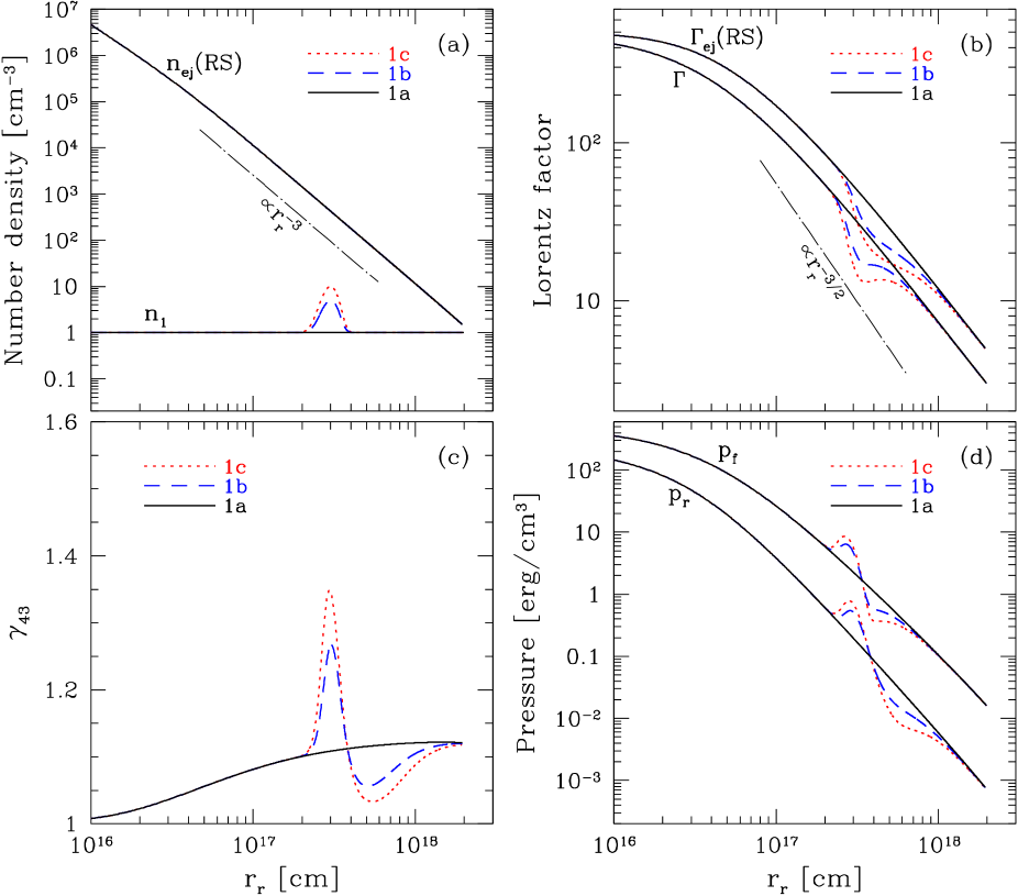
Figure 2: Blast wave dynamics of examples 1a, 1b, and 1c. The ambient medium density profile $n_{1}=\rho_{1}/m_{p}$ of each example is shown in panel (a) in different line (color) types. Panel (a) also shows the density $n_{\rm ej}{\rm(RS)}=\rho_{\rm ej}{\rm(RS)}/m_{p}$ of the ejecta shell that gets shocked by the RS when the RS is located at radius $r_{r}$. In panel (b), three curves labeled by $\Gamma_{\rm ej}{\rm(RS)}$ show the Lorentz factor of the ejecta shell that passes through the RS when the RS is at $r_{r}$. Three curves labeled by $\Gamma$ show the Lorentz factor of the blast wave as a function of the RS radius $r_{r}$. The relative Lorentz factor $\gamma_{43}$ between $\Gamma$ and $\Gamma_{\rm ej}{\rm(RS)}$ is shown in panel (c). Panel (d) shows the evolution of the RS pressure $p_{r}$ and FS pressure $p_{f}$ as a function of $r_{r}$.

The density profiles of the examples 1a, 1b, and 1c are shown together in the panel (a) of Figure 2; three different line (color) types are used to denote for each example, respectively. The panel (a) also shows the density $n_{\rm ej}{\rm(RS)}=\rho_{\rm ej}{\rm(RS)}/m_{p}$ of the ejecta shell that gets shocked by the RS when the RS is located at radius $r_{r}$. For a non-stratified ejecta, a simple spherical expansion leads to an $\propto r^{-2}$ decrease in the ejecta density. However, for a stratified ejecta, the ejecta density decreases faster than $\propto r^{-2}$ due to a radial spread-out of the evolving ejecta flow with a non-vanishing gradient $\Gamma_{\rm ej}^{\prime}(\tau)$. In the case of an exponential stratification of $\Gamma_{\rm ej}(\tau)$, U12 (Section 4.1) shows that $g_{\rm ej}(\tau)\equiv\left[-\,\frac{d}{d\tau}(\ln\Gamma_{\rm ej})\right]^{-1}$ has a constant value, and as a result, $n_{\rm ej}{\rm(RS)}\propto r_{r}^{-3}$ is satisfied for $g_{\rm ej}(\tau)\ll\frac{r}{c\Gamma_{\rm ej}^{2}}$. This behavior is shown in the panel (a). In the panel (b), the three curves labeled by $\Gamma_{\rm ej}{\rm(RS)}$ show the Lorentz factor of the ejecta shell that passes through the RS when the RS is at $r_{r}$. The three curves labeled by $\Gamma$ show the Lorentz factor of the blast wave as a function of the RS radius $r_{r}$. The relative Lorentz factor $\gamma_{43}$ between $\Gamma$ and $\Gamma_{\rm ej}{\rm(RS)}$ is shown in the panel (c). The $\gamma_{43}$ curve is a measure of the RS strength. Panel (d) shows the evolution of the RS pressure $p_{r}$ and FS pressure $p_{f}$ as a function of $r_{r}$.

The ejecta shells with low Lorentz factors run after the blast wave and gradually “catch up” with it at late times, adding their energy to the blast. Thus, the blast wave is continuously pushed, and its deceleration deviates from the self-similar solution of Blandford & McKee (1976); the $\Gamma$ curve of the example 1a shows that its blast wave decelerates slower than the BM solution $\Gamma\propto r_{r}^{-3/2}$. For the examples 1b and 1c, while encountering a density bump, the $p_{f}$ curve rises and as a consequence the $\Gamma$ curve decreases strongly. Then, the shell catching-up speeds up (as indicated by a strong rise in $\gamma_{43}$ curve) and quickly occurs for a wide range of ejecta shells (as shown by a fast decrease in $\Gamma_{\rm ej}{\rm(RS)}$ curve). The rise in $\gamma_{43}$ curve gives the rise in the $p_{r}$ curve. Now climbing down the density bump, the $p_{f}$ curve decreases rapidly. The $p_{f}$ curve goes even below the solid (black) curve of the example 1a since its blast wave has been decelerated significantly due to the bump encountering. The rapid decline in $p_{f}$ curve, together with adiabatic cooling of the blast wave, makes the $\Gamma$ curve start to recover from a fast decline phase; the $\Gamma_{\rm ej}{\rm(RS)}$ curve also starts to flatten, changing its shape to a concave curve. Consequently, the shell catching-up slows down and the $\gamma_{43}$ curve decreases, so does the $p_{r}$ curve.

Moving away from the bump region, the $p_{f}$ curve is still well below the solid (black) curve of the example 1a, retaining in memory the previous deceleration history due to the bump. The low FS pressure, combined with ongoing adiabatic cooling of the blast wave, makes the $\Gamma$ curve continue to recover; note that the $\Gamma$ curve of the example 1c exhibits a period of an actual acceleration of the blast wave. This continuing recovery in $\Gamma$ curve further slows down the shell catching-up and makes the $\gamma_{43}$ curve continue to decrease below the solid (black) curve. Accordingly, the $p_{r}$ curve also goes below the solid (black) curve. As the $p_{f}$ curve approaches back to the solid (black) curve, the recovery tendency in $\Gamma$ curve weakens and the $\gamma_{43}$ curve begins to rise again. Since the examples 1a, 1b, and 1c are given the same burst energy and ejecta stratification, the three $\Gamma$ curves, after all, should agree with one another, if the adiabatic conversion of internal energy has been properly taken care of. An important consistency test of whether the modeling is correct would be whether different models converge after the bump phase. An excellent agreement in $\Gamma$ curves as well as in other curves (i.e., $\Gamma_{\rm ej}{\rm(RS)}$, $\gamma_{43}$, $p_{f}$, and $p_{r}$ curves) is seen in Figure 2, suggesting the correctness of the modeling. Also, as described by the example 1c and other examples below, correct modeling should be able to capture an acceleration phase of the blast wave when the ambient medium density drops rapidly. Nava et al. (2013) also considered the role of adiabatic cooling and reproduced an acceleration phase of the blast wave.

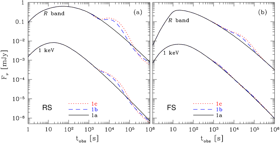
Figure 3: Afterglow light curves of examples 1a, 1b, and 1c. Panel (a) shows the RS emission in X-ray (1 keV) and R band as a function of the observer time $t_{\rm obs}$. Panel (b) shows the FS emission in X-ray (1 keV) and R band.

The afterglow light curves of the examples 1a, 1b, and 1c are shown in Figure 3. In panel (a), we show the RS emission in X-ray (1 keV) and R band as a function of the observer time $t_{\rm obs}$. In panel (b), we show the FS emission in X-ray (1 keV) and R band. The example 1a shows that, during the deceleration phase, the FS and RS light curves decline with a very similar value of decay indices; a detailed explanation regarding this point is given in U12. For the examples 1b and 1c, while encountering a density bump, a signature corresponding to the bump is visible on both the FS and the RS light curves, but with a stronger re-brightening feature imprinted on the RS light curves. The feature is stronger for the example 1c than for the example 1b, since the bump is bigger in the example 1c than in the example 1b. After exhibiting the re-brightening feature, the RS light curves go even below the solid (black) curve of the example 1a and then approach back to the solid (black) curve (just as the $\gamma_{43}$ curve behaves). This interesting behavior is not clearly present in the FS light curves.

3.2 Group (1a/1c/1d)

This group includes a new example 1d, whose density profile $n_{1}(r)$ in the ambient medium also has a Gaussian bump on top of the base density $n_{0}=1~{}\mbox{cm}^{-3}$ at the same location $r_{0}=3\times 10^{17}~{}\mbox{cm}$. The amplitude of the bump is $n_{a}=19~{}\mbox{cm}^{-3}$ so that the peak density is 20 times the base density. As for the spatial spread of the bump, we choose $\sigma$ such that the bump of the examples 1c and 1d contains a same amount of mass, $\int_{0}^{\infty}m_{p}\left[n_{1}(r)-n_{0}\right]4\pi r^{2}\,{\rm d}r$. Recalling that the example 1c has $n_{a}=9~{}\mbox{cm}^{-3}$ and $\sigma=\sigma_{0}=3\times 10^{16}~{}\mbox{cm}$, we obtain $\sigma$ for the example 1d, which is about $0.477\,\sigma_{0}$.

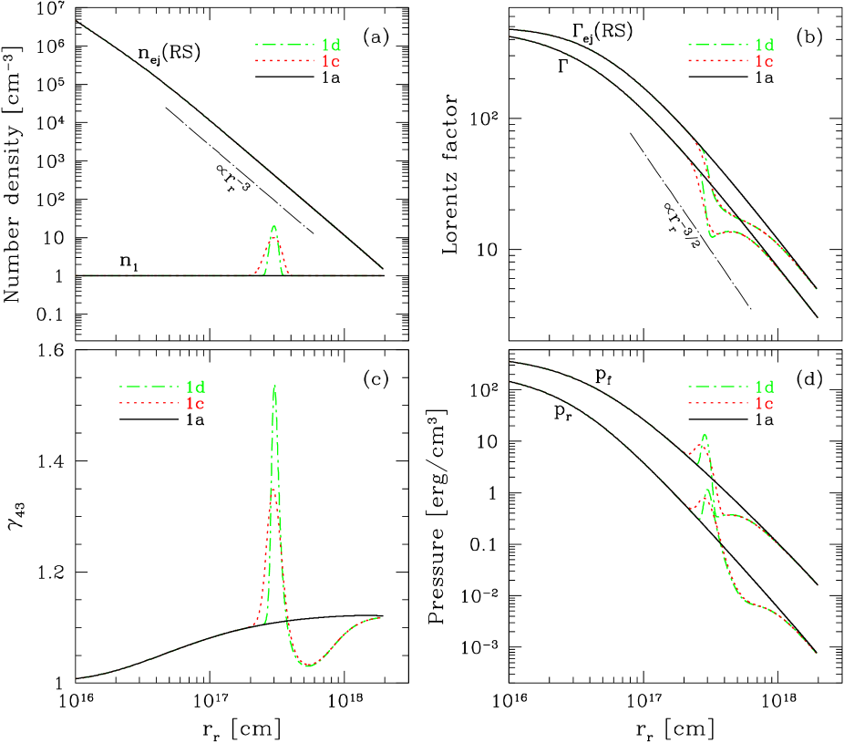
Figure 4: Same as in Figure 2, but for examples 1a, 1c, and 1d.

The blast wave dynamics of the examples 1a, 1c, and 1d are shown together in Figure 4; all 4 panels have the same notations as in the previous group (1a/1b/1c). One can read through the panels and understand the FS and RS dynamics, in the same way as we did above. In particular, we point out that since the examples 1c and 1d have the same mass contained in the bump, their dynamical evolution (i.e., $\Gamma$, $\Gamma_{\rm ej}{\rm(RS)}$, $\gamma_{43}$, $p_{f}$, and $p_{r}$ curves) agrees with each other as soon as their blast wave goes beyond the bump region (even before converging with the solid (black) curves of the example 1a). This agreement among examples with an equal bump mass serves as another consistency test.

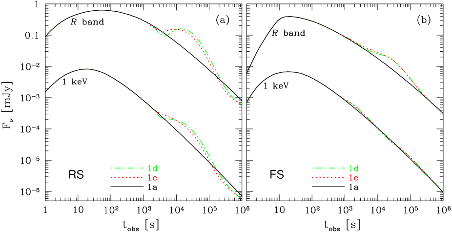
Figure 5: Same as in Figure 3, but for examples 1a, 1c, and 1d.

The afterglow light curves of the examples 1a, 1c, and 1d are shown together in Figure 5. Although the examples 1c and 1d have the same bump mass, the bump in the example 1d is narrower than in the example 1c. Accordingly, the RS light curves show a more concentrated re-brightening feature in the example 1d than in the example 1c. For the FS light curves, the difference between the two examples appears to be very small.

3.3 Group (1a/1e/1f)

The new examples 1e and 1f here have a density void in the ambient medium, located at radius $r_{0}$. A Gaussian shape is removed from our base density $n_{0}$ and thus the density profile is given by $n_{1}(r)=n_{0}-n_{a}\,e^{-(r-r_{0})^{2}/(2\sigma^{2})}$. For both examples 1e and 1f, we use a void amplitude $n_{a}=0.9~{}\mbox{cm}^{-3}$ so that the minimum density is 1/10 of the base density. As for the spatial spread of the void, the example 1e has $\sigma=\sigma_{0}$ while the example 1f has $\sigma=2\,\sigma_{0}$.

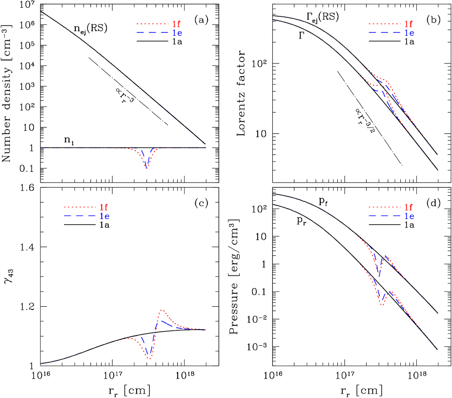
Figure 6: Same as in Figure 2, but for examples 1a, 1e, and 1f.

The blast wave dynamics of the examples 1a, 1e, and 1f are shown together in Figure 6. When the blast wave of the examples 1e and 1f encounters a density void shown in panel (a), its $p_{f}$ curve declines rapidly. This $p_{f}$ decline then, together with adiabatic cooling of the blast wave, makes the blast wave decelerate slowly, resulting in a flattening in the $\Gamma$ curve. As a result, the shell catching-up occurs slowly (as indicated by a flattening in the $\Gamma_{\rm ej}{\rm(RS)}$ curve and also by a decline in the $\gamma_{43}$ curve). The decline in the $\gamma_{43}$ curve gives the decline in the $p_{r}$ curve. Now climbing up the void hill (the outer side of void), the $p_{f}$ curve rises rapidly. The $p_{f}$ curve goes even above the solid (black) curve of the example 1a since its $\Gamma$ curve is above the solid (black) curve (due to the void encountering). The rapid rise in $p_{f}$ curve makes the $\Gamma$ curve start to turn into a fast decline phase; the $\Gamma_{\rm ej}{\rm(RS)}$ curve also changes its shape to a convex curve. Consequently, the shell catching-up speeds up and the $\gamma_{43}$ curve resumes rising. The $p_{r}$ curve also rises back as the $\gamma_{43}$ curve resumes rising.

Escaping from the void region, the $p_{f}$ curve is still above the solid (black) curve of the example 1a, retaining the memory of the previous history of void encountering. The high FS pressure makes the $\Gamma$ curve continue to decline fast and thus makes the $\gamma_{43}$ curve continue to rise above the solid (black) curve. Hence, the $p_{r}$ curve also goes above the solid (black) curve. As the $p_{f}$ curve gradually approaches back to the solid (black) curve, the fast-decline tendency in $\Gamma$ curve weakens and therefore the $\gamma_{43}$ curve begins to decrease again. For the same reason we discussed above for bumps, the blast wave evolution (i.e., $\Gamma$, $\Gamma_{\rm ej}{\rm(RS)}$, $\gamma_{43}$, $p_{f}$, and $p_{r}$ curves) of these three examples 1a, 1e, and 1f should agree with one another, after all. The agreement shown in Figure 6, while invoking for density voids, also serves as a consistency test for the correctness of modeling.

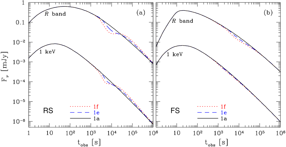
Figure 7: Same as in Figure 3, but for examples 1a, 1e, and 1f.

The afterglow light curves of the examples 1a, 1e, and 1f are shown in Figure 7. For the examples 1e and 1f, while encountering a density void, a dip signature corresponding to the void is visible on both the FS and the RS light curves, but with a stronger feature imprinted on the RS light curves. The feature is stronger for the example 1f than for the example 1e, since the void is bigger in the example 1f than in the example 1e. After exhibiting the dip feature, the RS light curves go even above the solid (black) curve of the example 1a and then approach back to the solid (black) curve, just as the $\gamma_{43}$ curve behaves. This behavior is not present in the FS light curves.

3.4 Group (1a/1f/1g)

The new example 1g here has a density void in the ambient medium at the same location $r_{0}$. Its density profile is given by $n_{1}(r)=n_{0}-n_{a}\,e^{-(r-r_{0})^{4}/(4\sigma^{4})}$, with the void amplitude $n_{a}=0.95~{}\mbox{cm}^{-3}$ so that the minimum density is 1/20 of the base density $n_{0}$. We choose $\sigma$ such that the examples 1f and 1g have a same value for the integration $\int_{0}^{\infty}m_{p}\left[n_{1}(r)-n_{0}\right]4\pi r^{2}\,{\rm d}r$, to ensure that an equal amount of mass is reduced by the void in the examples 1f and 1g. Note that we use a boxier shape of functional form for the void of the example 1g, so that an equality of the integration above gives a narrower void for the example 1g.

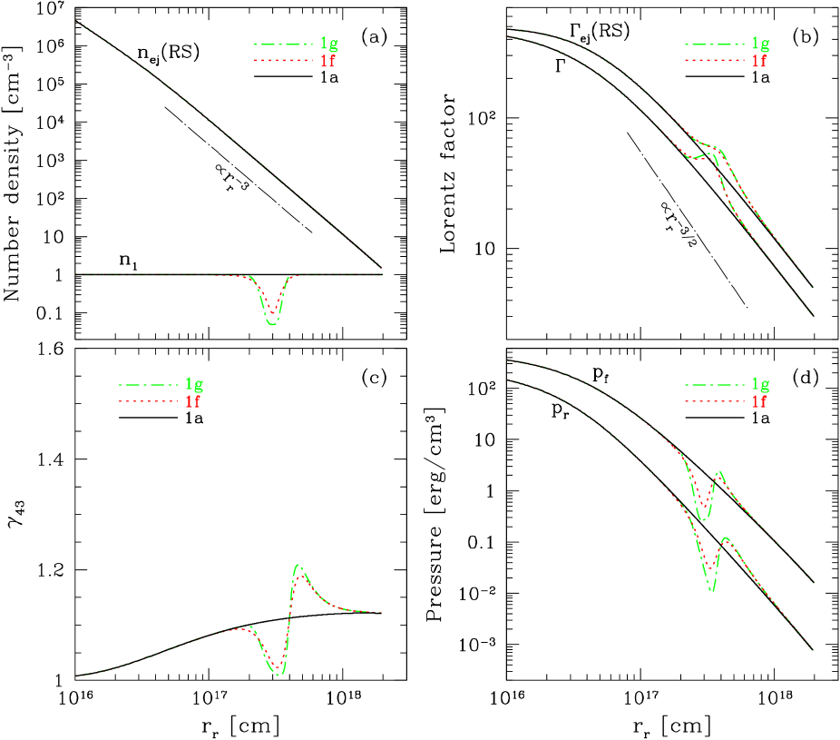
Figure 8: Same as in Figure 2, but for examples 1a, 1f, and 1g.

The blast wave dynamics of the examples 1a, 1f, and 1g are shown together in Figure 8. Again, one can read through the panels and understand the FS and RS dynamics. Note that the $\Gamma$ curve of the example 1g shows a period of an actual acceleration of the blast wave. Since the void of the examples 1f and 1g reduces an equal amount of mass from the base, the blast wave evolution of these two examples agrees with each other as soon as their blast wave goes beyond the void region, even before converging with the solid (black) curves of the example 1a. This serves as another consistency test.

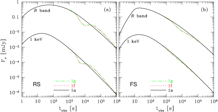
Figure 9: Same as in Figure 3, but for examples 1a, 1f, and 1g.

The afterglow light curves of the examples 1a, 1f, and 1g are shown together in Figure 9. The examples 1f and 1g show a small difference on the RS light curves, while almost no difference on the FS light curves is observed between these two examples.

3.5 Group (1a/1h/1i)

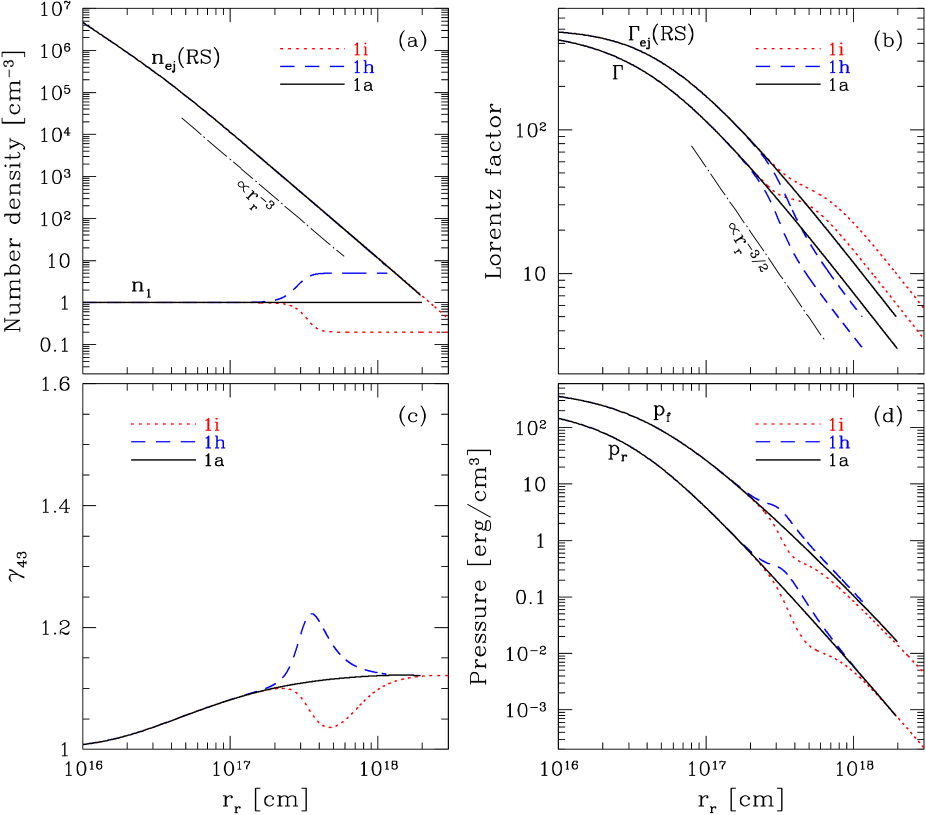
Figure 10: Same as in Figure 2, but for examples 1a, 1h, and 1i.

The new examples 1h and 1i invoke a step-like density structure. The example 1h has a density profile $n_{1}(r)=n_{0}+n_{a}\,[1+e^{-(r-r_{0})/\sigma_{0}}]^{-1}$, with an amplitude $n_{a}=4~{}\mbox{cm}^{-3}$. The density increases from the base $n_{0}$ by a factor of 5, through the step that is located at a radius $r_{0}$ in a length scale $\sigma_{0}$. The example 1i has the same density profile except that $n_{a}=-0.8~{}\mbox{cm}^{-3}$. Then, the density decreases from the base by a factor of 5. See panel (a) in Figure 10.

The blast wave dynamics of the examples 1a, 1h, and 1i are shown together in Figure 10. For the example 1h, while encountering the rising step, the blast wave shows the same behavior as in the rising phase of the bumps. However, after that there is no rapid decline in the density and thus no rapid decline in the $p_{f}$ curve. Therefore, the $\Gamma$ curve does not recover from the fast decline and stay well below the solid (black) curve. Propagating further on a constant density medium lifted up from the base, the blast wave gradually stabilizes and the $\gamma_{43}$ curve returns back to the solid (black) curve, so does the $p_{r}$ curve. The $p_{f}$ curve also approaches back to the solid (black) curve (propagating with lower $\Gamma$ at higher $n_{1}$ region), but does not agree with the solid (black) curve. Similarly, for the example 1i, while encountering the descending step, the blast wave shows the same behavior as in the descending phase of the voids. Again, after that there is no rapid rise in density and thus no rapid rise in the $p_{f}$ curve. Hence, the $\Gamma$ curve does not turn into a rapid decline phase and stay well above the solid (black) curve. Moving further on a constant density medium shifted down from the base, the blast wave gradually adjusts to the lower step and the $\gamma_{43}$ curve returns to the solid (black) curve, so does the $p_{r}$ curve. The $p_{f}$ curve also approaches back to the solid (black) curve (propagating with higher $\Gamma$ at lower $n_{1}$ region), but does not completely agree with the solid (black) curve.

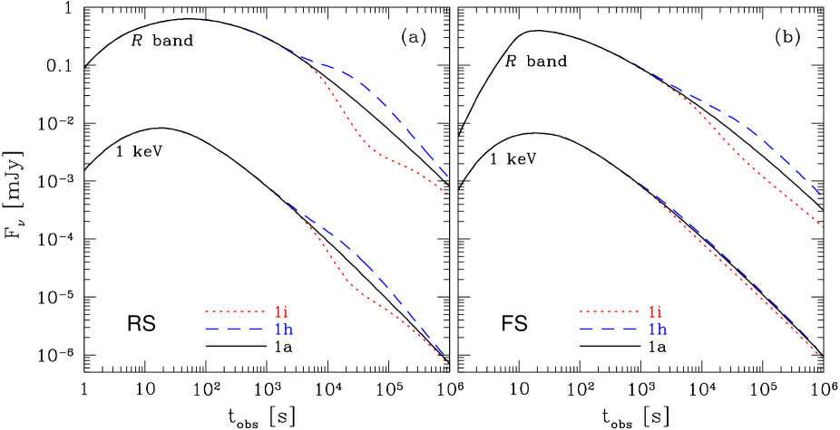
Figure 11: Same as in Figure 3, but for examples 1a, 1h, and 1i.

The afterglow light curves of the examples 1a, 1h, and 1i are shown together in Figure 11. For the example 1h, the RS light curves show a mild re-brightening and then approach back to the solid (black) curve. The FS light curves also respond to the rising phase of the step structure, but do not approach back to the solid (black) curve. For the example 1i, the RS light curves decline initially, responding to the descending phase of the step structure, and then go back to the solid (black) curve. Note that this kind of behavior in light curves has often been interpreted as an FS wave exhibiting a jet break (for the initial steepening), followed by a late-time energy injection (for the flattening). Here we present a simple way to reproduce such a behavior, i.e., an RS wave responding to a descending step structure. The FS light curves of the example 1i also respond to the step, but again do not approach back to the solid (black) curve.

3.6 Group (2a/2c/2d)

As mentioned above, the examples with the number 2 in their names have a short-lived RS, with a constant ejecta Lorentz factor $\Gamma_{\rm ej}=300$. For the external ambient medium, three examples 2a, 2c, and 2d here share the same density profile with the examples 1a, 1c, and 1d, respectively. Recall that the example 1a has a constant density $n_{0}$ (our base), and the examples 1c and 1d have a density bump on top of the base.

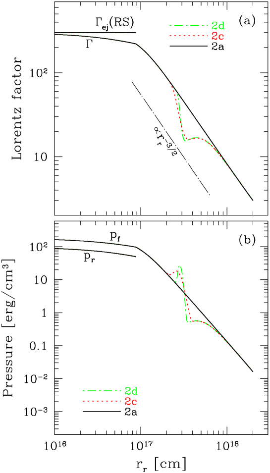
Figure 12: Blast wave dynamics of examples 2a, 2c, and 2d. These examples have a short-lived RS. The same notations as in Figure 2 are used here. Panel (a) shows the $\Gamma$ and $\Gamma_{\rm ej}{\rm(RS)}$ curves, and the panel (b) shows the $p_{f}$ and $p_{r}$ curves.

In Figure 12, we show the blast wave dynamics of the examples 2a, 2c, and 2d together. The notations are the same as in the previous groups of examples with a long-lived RS. We show the $\Gamma$ and $\Gamma_{\rm ej}{\rm(RS)}$ curves in the panel (a) and the $p_{f}$ and $p_{r}$ curves in the panel (b). The $\Gamma_{\rm ej}{\rm(RS)}$ and $p_{r}$ curves exhibit an early end when the RS crosses the end of the ejecta. After that, there is no more ejecta shells catching up with the blast wave. Hence, the $\Gamma$ curve of the example 2a transitions to and then agrees with the Blandford-McKee deceleration. For the examples 2c and 2d, the FS dynamics (i.e., $\Gamma$ and $p_{f}$ curves) responding to the density bump can be understood in the same way as in the group (1a/1c/1d). An early agreement between 2c and 2d curves beyond the bump region is observed again since the bump in those two examples contains a same amount of mass. It is also observed that all three examples 2a, 2c, and 2d agree with one another in the FS curves as their blast wave propagates further away from the bump region, suggesting the correctness of our modeling. These agreements serve as a consistency test here.

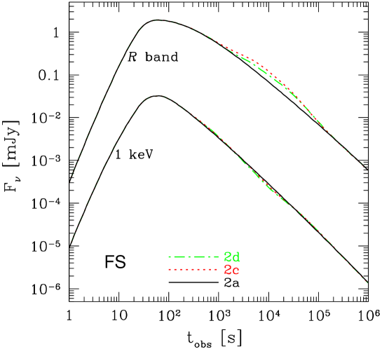
Figure 13: Afterglow light curves of examples 2a, 2c, and 2d. The FS emission in X-ray (1 keV) and R band is shown as a function of the observer time $t_{\rm obs}$.

In Figure 13, we show the FS light curves of the examples 2a, 2c, and 2d together. For the examples 2c and 2d, the FS light curves responding to the density bump exhibit the same behavior as in the group (1a/1c/1d).

3.7 Group (2a/2f/2g)

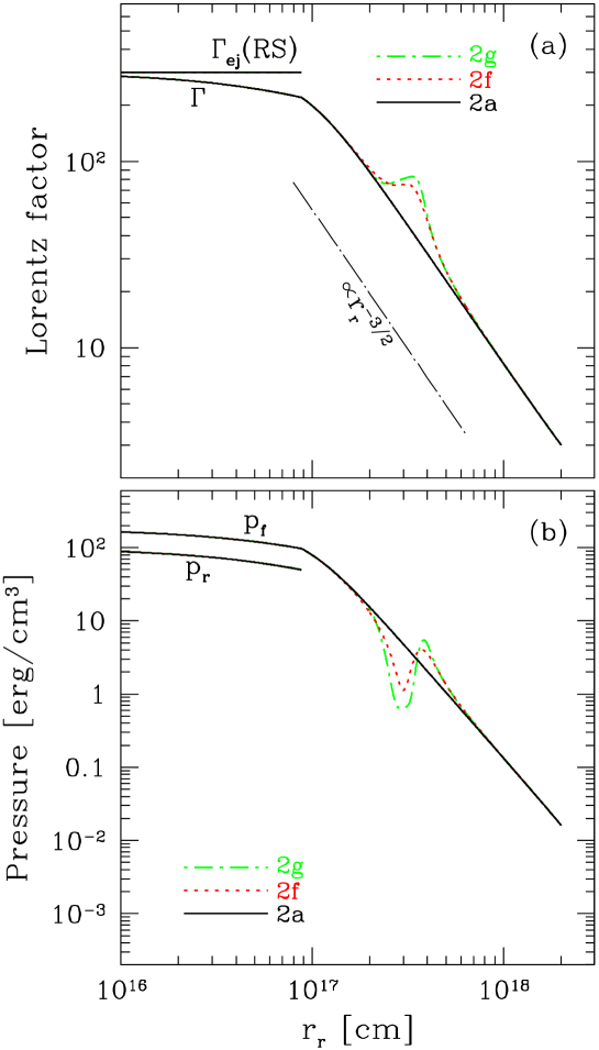
Figure 14: Same as in Figure 12, but for examples 2a, 2f, and 2g.

The new examples 2f and 2g share the same density profile with the examples 1f and 1g, respectively. Recall that the examples 1f and 1g have a density void in the ambient medium. In Figure 14, we show the blast wave dynamics of the examples 2a, 2f, and 2g together. For the examples 2f and 2g, the FS dynamics (i.e., $\Gamma$ and $p_{f}$ curves) responding to the density void can be understood in the same way as in the group (1a/1f/1g). An early agreement between 2f and 2g curves beyond the void region is observed since the void in those two examples reduces a same amount of mass from the base. Also, all three examples 2a, 2f, and 2g agree with one another in the FS curves as their blast wave propagates further away from the void region, suggesting the correctness of the modeling.

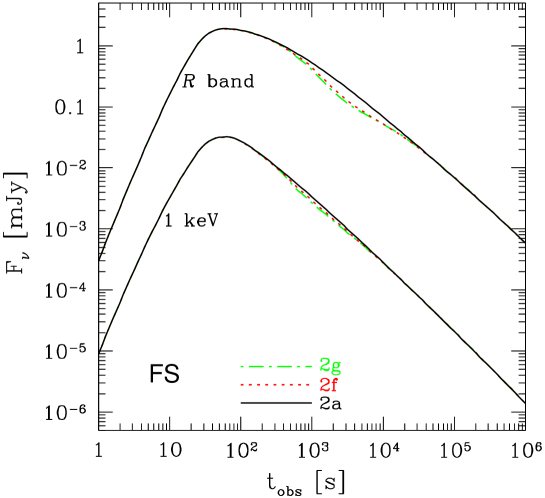
Figure 15: Same as in Figure 13, but for examples 2a, 2f, and 2g.

In Figure 15, we show the FS light curves of the examples 2a, 2f, and 2g together. For the examples 2f and 2g, the FS light curves responding to the density void exhibit the same behavior as in the group (1a/1f/1g).

4 Conclusions and Discussion

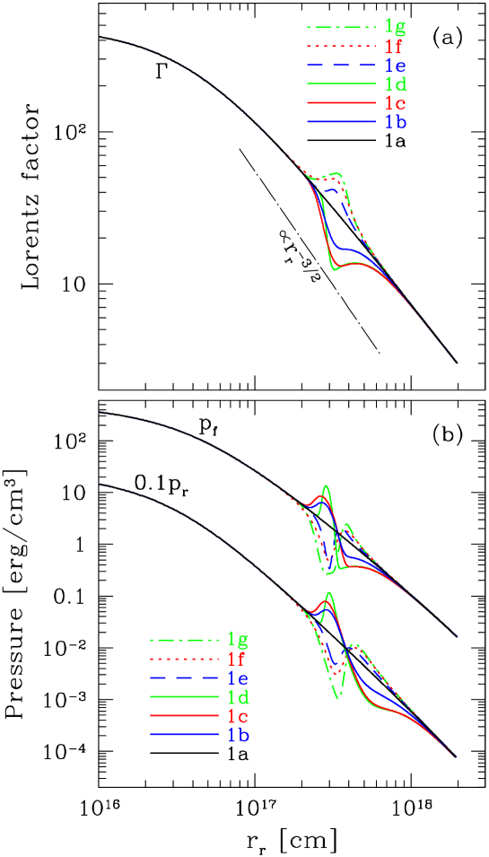
Figure 16: Shown together is the blast wave dynamics of examples 1a, 1b, 1c, 1d, 1e, 1f, and 1g. The notations are the same as in Figure 2. Panel (a) shows the $\Gamma$ curves, and the panel (b) shows the $p_{f}$ and $p_{r}$ curves. The $p_{r}$ curves are multiplied by a factor of 0.1, in order to avoid an overlap with the $p_{f}$ curves.

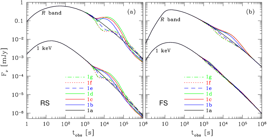
Figure 17: Same as in Figure 3, but for examples 1a, 1b, 1c, 1d, 1e, 1f, and 1g.

In this paper, we have investigated the blast wave dynamics and afterglow light curves of a GRB blast wave encountering various density structures in the surrounding ambient medium. We use the semi-analytic formulation of relativistic blast waves (presented in U11) to find an accurate numerical solution for both the FS and RS dynamics and employ the Lagrangian description of the blast waves (presented in U12) to perform a sophisticated calculation of afterglow emission. In particular, we consider numerical examples with density bumps, voids, or steps in the ambient medium and present their FS and RS dynamics and light curves. We form groups of examples in order to provide an efficient comparison among them and to help readers understand how the FS and RS dynamics should behave when the blast waves encounter those density structures. Giving a detailed explanation on their dynamics, we stress on the important role of adiabatic cooling of blast waves and then propose a number of consistency tests that correct modeling of blast waves needs to satisfy. We also present examples with a short-lived RS and show that the same consistency tests need to be satisfied for the FS dynamics. All these tests should serve as an accuracy indicator for any future (analytical, numerical, or hydrodynamical) modeling of blast waves with a long/short-lived RS. We point out that the RS dynamics responding to density structures in the ambient medium is studied extensively for the first time here. Also, the FS dynamics responding to density voids is presented here for the first time. As a summary, in Figure 16, we show together the blast wave dynamics of examples with a long-lived RS for bumps (i.e., 1b, 1c, and 1d) and voids (i.e., 1e, 1f, and 1g); the example 1a with our constant base density is also shown together. The FS and RS dynamics exhibit again an excellent agreement among examples beyond the bump/void region. In Figure 17, we show together the FS and RS light curves of these 7 examples. It appears that the RS light curves can produce some interesting observed features such as re-brightenings, dips, and slow wiggles, while the FS light curves in general produce weaker and smoother features, which may not be able to interpret significant bumps and wiggles observed in some afterglows.

Why does the bump/void leave such a different imprint on the FS and RS light curves? The question is intriguing since the $p_{f}$ and $p_{r}$ curves exhibit a similar degree of response signature for bumps or voids (as one can see from Figure 16). We first recall that different microphysics parameters are adopted for the FS and RS; $\epsilon_{e}=10^{-1}$ and $\epsilon_{B}=10^{-2}$ for the RS light curves and $\epsilon_{e}=10^{-2}$ and $\epsilon_{B}=10^{-4}$ for the FS light curves, so that the FS and RS spectral density fluxes become comparable to each other. As a first step, we examine the effect of microphysics parameters on the response feature. In general, a higher value of $\epsilon_{e}$ or $\epsilon_{B}$ gives a weaker response signature on both the FS and the RS light curves. If we increase $\epsilon_{e}$, the Compton parameter $Y$ increases, which makes the electrons cool faster. If we increase $\epsilon_{B}$, the magnetic field strength $B$ increases, which also makes the electrons cool faster. In either case, the cooling Lorentz factor of our Lagrangian shells decreases faster. As a result, a smaller number of recently shocked shells have the electrons that can contribute to the X-ray or R band emission. In other words, for a higher $\epsilon_{e}$ or $\epsilon_{B}$ value, a smaller region of the blast wave responds to bumps or voids, leaving a weaker signature on the light curves. Conversely, a lower value of $\epsilon_{e}$ or $\epsilon_{B}$ gives a stronger response signature on both the FS and the RS light curves. For the same parameters $\epsilon_{e}=10^{-1}$ and $\epsilon_{B}=10^{-3}$ adopted for both shocked regions, the RS light curves show a stronger signature than in Figure 17 whereas the FS light curves show an even weaker (nearly negligible) signature than in Figure 17. Therefore, the different microphysics parameters that we adopted for the FS and RS regions do not provide an explanation for the question. In fact, the microphysics parameters are chosen in such a way that the bump/void signature becomes enhanced on the FS light curves as compared to the RS light curves.

The different signatures imprinted on the FS and RS light curves can be mainly understood by considering the influence of injection Lorentz factor of electrons. As the blast wave encounters density bumps, the $p_{f}$ curve rises, but the $\Gamma$ curve declines, which decreases the injection Lorentz factors in the FS fresh shells. Hence, there is competition between the rising energy density of shocked gas and the declining injection energy of electrons in the FS region. On the other hand, while encountering density bumps, the $p_{r}$ and $\gamma_{43}$ curves rise together. Thus, there is synergy between the rising energy density of shocked gas and the rising injection energy of electrons in the RS region. Similarly, as the blast wave encounters density voids, the FS region has competition between the decreasing energy density of shocked gas and the flattening (or increasing) injection energy of electrons. The RS region has again synergy between the declining energy density of shocked gas and the decreasing injection energy of electrons. This is the main source of the FS/RS asymmetry in response to the bump/void structures in the ambient medium.

Another (secondary) reason for different imprints on the FS and RS comes from the intrinsic difference of the FS and RS propagation direction in the co-moving fluid frame. The FS propagates forward in the co-moving frame, so that the photons emitted from fresh shells are “mixed” together with the photons coming from old shells inside the shocked region. This photon mixing among the fresh and old shells tends to smooth out the bump/void signature in the FS light curves. On the other hand, the RS propagates backward in the co-moving frame, so that the photons emitted from fresh shells should arrive later than the photons coming from old shells inside the shocked region. Thus, there is no photon mixing among the fresh and old shells, which helps the RS light curves keep the bump/void signature.

The FS/RS asymmetry presented in this paper provides an important insight on the origin of afterglow emission. In reality, the observed light curves do not distinguish the contribution of the RS from the FS. In the standard framework of afterglow production by a blast wave with a short-lived RS, the contribution from the RS region after the RS crossing the end of the ejecta has a distinguishable temporal index ($\sim-2$) in the observed light curves. However, when a blast wave with a long-lived RS is considered, the contribution from the RS region can not be easily distinguished from the FS contribution by simply looking at the temporal index of the observed light curves. Under these circumstances, one possible way to distinguish one from the other would be to investigate in detail their response features due to the inhomogenities in the ambient medium (as we do here in this paper) or in the ejecta stratification (as presented in U12). As we showed in this paper and U12, these inhomogenities generally leave a lot stronger signatures in the RS light curves than in the FS light curves. Therefore, these results suggest that the observed light curves with strong features favor toward the RS origin. One may think that the FS emission could account for some weak features. We believe that the spectral evolution of the FS and RS emission during the bump/void encounters may help further distinguish one from the other in the future, which will be investigated elsewhere. For the observed light curves without any noticeable feature, we believe that the future measurements of “polarization degree curves” for a longer time scale, say, up to hours or days, would hold a key to distinguish the contribution of the RS from the FS.

We also add another important remark regarding the possibility to differentiate between the two popular scenarios to account for the observed light curve features, i.e., the inhomogenities in the ambient medium (the current paper) or in the ejecta structure (U12). These two popular scenarios in fact give rise to different signatures. It appears that, for the RS emission, the inhomogenities in the ambient medium leave a stronger feature in the optical light curves than in the X-ray light curves, whereas the inhomogenities in the ejecta structure leave a stronger feature in the X-ray light curves than in the optical light curves. This tendency is shown in the current paper and U12, but requires a more detailed investigation to enable a better understanding on the underlying physics. If this is indeed the case, and if the observed emission is dominated by the RS emission, then the multi-wavelength afterglow observations will be able to differentiate the two scenarios.

The bump/void structures presented in our models are essentially concentric shells of high or low density medium stacked upon each other. However, in reality, these structures should be three dimensional in nature, surrounded by an inter-clump medium (ICM). This 3-D aspect of the structures would then significantly alter the dynamics of the blast wave. It can be expected that the blast wave dynamics can be dominated by the uniform ICM rather than the bump/void structures if the clumps of these structures are sufficiently small. In this case, however, those small clumps would not leave significant features anyway, and the observed light curves would be dominated by the uniform ICM. For large clumps that could considerably affect the blast wave dynamics, we believe that our models can still reasonably apply when the clumps along the line of sight are as big as the visible area with an angular size $\sim 1/\Gamma$.

We also studied the step-like density structures in the paper. These structures may exist as a consequence of pre-ejection history from the central engine. When the relativistic blast wave encounters previously-ejected slowly moving denser shells, these shells could act as an ascending step-like structure. When the blast wave exits these denser shells, it experiences a descending step structure. In the case of a wind environment, a rapid change in the mass-loss rate in the past could create a step-like density structure. Note that these situations would probably create a relatively spherical density structure when viewed from the jetted blast wave. We stress that a descending step structure is proposed here to give a natural explanation for a dip feature – a steepening followed by a flattening – in GRB light curves.

Figure 1: Stratification of the ejecta Lorentz factor $\Gamma_{\rm ej}$ as a function of ejection time $\tau$ for numerical examples 1a, 1b, 1c, 1d, 1e, 1f, 1g, 1h, and 1i. These 9 examples have a long-lived RS.

References

- Blandford & McKee (1976) Blandford, R. D., & McKee, C. F. 1976, Physics of Fluids, 19, 1130
- Chevalier & Li (2000) Chevalier, R. A., & Li, Z.-Y. 2000, ApJ, 536, 195
- Dai (2004) Dai, Z. G. 2004, ApJ, 606, 1000
- Dai & Lu (2002) Dai, Z. G., & Lu, T. 2002, ApJ, 565, L87
- Dai & Wu (2003) Dai, Z. G., & Wu, X. F. 2003, ApJ, 591, L21
- Gao et al. (2013) Gao, H., Lei, W.-H., Zou, Y.-C., Wu, X.-F., & Zhang, B. 2013, New A Rev., 57, 141
- Gat et al. (2013) Gat, I., van Eerten, H., & MacFadyen, A. 2013, ApJ, 773, 2
- Genet et al. (2007) Genet, F., Daigne, F., & Mochkovitch, R. 2007, MNRAS, 381, 732
- Holland et al. (2003) Holland, S. T., Weidinger, M., Fynbo, J. P. U., et al. 2003, AJ, 125, 2291
- Lazzati et al. (2002) Lazzati, D., Rossi, E., Covino, S., Ghisellini, G., & Malesani, D. 2002, A&A, 396, L5
- Lipkin et al. (2004) Lipkin, Y. M., Ofek, E. O., Gal-Yam, A., et al. 2004, ApJ, 606, 381
- Mészáros & Rees (1997) Mészáros, P., & Rees, M. J. 1997, ApJ, 476, 232
- Nakar & Granot (2007) Nakar, E., & Granot, J. 2007, MNRAS, 380, 1744
- Nava et al. (2013) Nava, L., Sironi, L., Ghisellini, G., et al. 2013, MNRAS, 433, 2107
- Rees & Mészáros (1998) Rees, M. J., & Mészáros, P. 1998, ApJ, 496, L1+
- Sari & Mészáros (2000) Sari, R., & Mészáros, P. 2000, ApJ, 535, L33
- Sari et al. (1998) Sari, R., Piran, T., & Narayan, R. 1998, ApJ, 497, L17+
- Uhm (2011) Uhm, Z. L. 2011, ApJ, 733, 86 (U11)
- Uhm & Beloborodov (2007) Uhm, Z. L., & Beloborodov, A. M. 2007, ApJ, 665, L93
- Uhm & Zhang (2014) Uhm, Z. L., & Zhang, B. 2014, ApJ, 780, 82
- Uhm et al. (2012) Uhm, Z. L., Zhang, B., Hascoët, R., et al. 2012, ApJ, 761, 147 (U12)
- Zhang & Mészáros (2001) Zhang, B., & Mészáros, P. 2001, ApJ, 552, L35