Prospects for electron spin–dependent short–range force experiments with rare earth iron garnet test masses

Abstract

A study of the possible interactions between fermions assuming only rotational invariance has revealed 15 forms for the potential involving the fermion spins. We review the experimental constraints on unobserved macroscopic, spin–dependent interactions between electrons in the range below 1 cm. An existing experiment, using 1 kHz mechanical oscillators as test masses, has been used to constrain mass–coupled forces in this range. With suitable modifications, including spin–polarized test masses, this experiment can be used to explore all 15 possible spin–dependent interactions between electrons in this range with unprecedented sensitivity. Samples of ferrimagnetic dysprosium iron garnet have been fabricated in the suitable test mass geometry and shown to have spin densities on the order of 10${}^{20}\hbar$/cm³ with very low intrinsic magnetism.

I Introduction

The possible existence of unobserved interactions of nature with ranges from microns to millimeters and very weak couplings to matter has begun to attract a great deal of scientific attention. Many theories beyond the Standard Model possess extended symmetries that, when broken at high energy scales, lead to weakly coupled, light bosons such as axions, familons, and Majorons, which can generate relatively long–range interactions Beringer et al. (2012). Several theoretical attempts to explain dark matter and dark energy also produce new weakly coupled long–range interactions. The fact that the dark energy density, of order (1 meV)⁴, corresponds to a length scale of $\sim$100 $\mu$m encourages searches for new phenomena at this scale in particular Adelberger et al. (2009). Particles which might transmit such interactions are sometimes referred to generically as WISPs (Weakly-Interacting Sub-eV Particles) Jaeckel and Ringwald (2010) in recent theoretical literature, or as “portals” to a hidden sector Pospelov et al. (2008).

A general classification of interactions between non-relativistic fermions assuming only rotational invariance reveals 16 different operator structures Dobrescu and Mocioiu (2006). Of these, 15 involve the spin of at least one of the particles and 7 their relative momentum. In general, experimental constraints on unobserved interactions that depend on the spin and/or velocity of the particles are fewer and less stringent than those for static, spin–independent interactions Adelberger et al. (2009). However, new experimental results from initial searches for the former interactions have accelerated over the last few years. In particular, the velocity–dependent interactions involving the spin of both particles have been constrained at long range using the geomagnetic field Hunter and Ang (2013), and at the atomic scale from an analysis of spin–exchange interactions Kimball et al. (2010).

One approach to the search for short–range forces uses planar, 1 kHz mechanical oscillators as test masses with a stiff conducting shield in between them to suppress backgrounds Long et al. (2003). A fully–constructed experiment in the lab of the authors uses tungsten test masses to search for mass–coupled forces in the range below 1 mm. With modifications including spin–polarized test masses, this technique can be used to create localized spin sources in close proximity with non-zero relative velocity. It thus has the capability to probe essentially all of the spin and velocity–dependent interactions described in Dobrescu and Mocioiu (2006), with unprecedented sensitivity in the range of interest. Ferrimagnetic rare earth iron garnets show promise as spin–polarized test masses with low intrinsic magnetism, and several samples have been fabricated in the suitable geometry.

This paper is organized as follows. Sec. II reviews the parameterization in Dobrescu and Mocioiu (2006), as applied to the proposed spin–dependent force search. The current short–range limits on polarized electron interactions are reviewed in Sec. III. The experiment, with details on polarized test masses made from dysprosium iron garnet, is described in Sec. IV. Sensitivity calculations based on the available test masses are presented in Sec. V.

II Parameterization

In the non–relativistic, zero–momentum transfer limit, the long–range potential $V_{i}$ ($i$ = 1,…,16) in the general classification in Dobrescu and Mocioiu (2006) for single boson exchange depends (in the enumeration in Dobrescu and Mocioiu (2006)) on 72 dimensionless coupling constants $f_{i}^{1,2}$. Here, the superscripts denote the species of interacting fermions.

In the experiment described in Sec. IV, the polarized particles (that is, the particles with non-zero projection of spin averaged over the volumes of the test masses) are electrons. There are nine components of the spin–spin potential between two polarized electrons. Three are static, given (in SI units, and adopting the numbering scheme in Dobrescu and Mocioiu (2006)) by:

$$V_{2} = f_{2}^{ee}\frac{\hbar c}{4\pi}(\hat{\sigma}_{1}\cdot\hat{\sigma}_{2})\left(\frac{1}{r}\right)e^{-r/\lambda}$$

$$V_{3} = f_{3}^{ee}\frac{\hbar^{3}}{4\pi m_{e}^{2}c}\left[(\hat{\sigma}_{1}\cdot\hat{\sigma}_{2})\left(\frac{1}{\lambda r^{2}}+\frac{1}{r^{3}}\right)-(\hat{\sigma}_{1}\cdot\hat{r})(\hat{\sigma}_{2}\cdot\hat{r})\left(\frac{1}{\lambda^{2}r}+\frac{3}{\lambda r^{2}}+\frac{3}{r^{3}}\right)\right]e^{-r/\lambda}$$

$$V_{11} = -f_{11}^{ee}\frac{\hbar^{2}}{4\pi m_{e}}\left[(\hat{\sigma}_{1}\times\hat{\sigma}_{2})\cdot\hat{r}\right]\left(\frac{1}{\lambda r}+\frac{1}{r^{2}}\right)e^{-r/\lambda}.$$ (1)

Here, ${\vec{s}_{1,2}}=\hbar\hat{\sigma}_{1,2}/2$ are the spins of electrons (in test masses 1 and 2), $\hat{r}=\vec{r}/r$ is the unit vector along the direction between them, $\hbar$ is Planck’s constant, $c$ is the speed of light in vacuum, $m_{e}$ is the electron mass, and $\lambda$ is the interaction range. The remaining six components depend on the relative velocity $\vec{v}$ of the electrons:

$$V_{6+7} = -f_{6+7}^{ee}\frac{\hbar^{2}}{4\pi m_{e}c}\left[(\hat{\sigma}_{1}\cdot\vec{v})(\hat{\sigma}_{2}\cdot\hat{r})\right]\left(\frac{1}{\lambda r}+\frac{1}{r^{2}}\right)e^{-r/\lambda}$$

$$V_{8} = f_{8}^{ee}\frac{\hbar}{4\pi c}\left[(\hat{\sigma}_{1}\cdot\vec{v})(\hat{\sigma}_{2}\cdot\vec{v})\right]\left(\frac{1}{r}\right)e^{-r/\lambda}$$

$$V_{14} = f_{14}^{ee}\frac{\hbar}{4\pi}\left[\left(\hat{\sigma}_{1}\times\hat{\sigma}_{2}\right)\cdot\vec{v}\right]\left(\frac{1}{r}\right)e^{-r/\lambda}$$

$$V_{15} = -f_{15}^{ee}\frac{\hbar^{3}}{8\pi m_{e}^{2}c^{2}}\left\{\left[\hat{\sigma}_{1}\cdot(\vec{v}\times\hat{r})\right](\hat{\sigma}_{2}\cdot\hat{r})+(\hat{\sigma}_{1}\cdot\hat{r})\left[\hat{\sigma}_{2}\cdot(\vec{v}\times\hat{r})\right]\right\}\left(\frac{1}{\lambda^{2}r}+\frac{3}{\lambda r^{2}}+\frac{3}{r^{3}}\right)e^{-r/\lambda}$$

$$V_{16} = -f_{16}^{ee}\frac{\hbar^{2}}{8\pi m_{e}c^{2}}\left\{\left[\hat{\sigma}_{1}\cdot(\vec{v}\times\hat{r})\right](\hat{\sigma}_{2}\cdot\vec{v})+(\hat{\sigma}_{1}\cdot\vec{v})\left[\hat{\sigma}_{2}\cdot(\vec{v}\times\hat{r})\right]\right\}\left(\frac{1}{\lambda r}+\frac{1}{r^{2}}\right)e^{-r/\lambda}.$$ (2)

There are six components in the case where only one test mass is polarized. The potentials between a polarized electron and an unpolarized atom of atomic number $Z$ and mass number $A$ are given by:

$$V_{4+5} = -Z\left[f_{\perp}^{ee}+f_{\perp}^{ep}+\left(\frac{A-Z}{Z}\right)f_{\perp}^{en}\right]\frac{\hbar^{2}}{8\pi m_{e}c}\left[\hat{\sigma}_{1}\cdot(\vec{v}\times\hat{r})\right]\left(\frac{1}{\lambda r}+\frac{1}{r^{2}}\right)e^{-r/\lambda}$$

$$V_{9+10} = Z\left[f_{r}^{ee}+f_{r}^{ep}+\left(\frac{A-Z}{Z}\right)f_{r}^{en}\right]\frac{\hbar^{2}}{8\pi m_{e}}(\hat{\sigma}_{1}\cdot\hat{r})\left(\frac{1}{\lambda r}+\frac{1}{r^{2}}\right)e^{-r/\lambda}$$

$$V_{12+13} = Z\left[f_{v}^{ee}+f_{v}^{ep}+\left(\frac{A-Z}{Z}\right)f_{v}^{en}\right]\frac{\hbar}{8\pi}(\hat{\sigma}_{1}\cdot\vec{v})\left(\frac{1}{r}\right)e^{-r/\lambda},$$ (3)

where $\hat{r}$ points from the electron to the atom and $\vec{v}$ is their relative velocity. Following Dobrescu and Mocioiu (2006), only one linear combination of the separate components in Eq. 3 has been used (as in the expression for $V_{6+7}$ in Eq. 2), and the coupling constants are given in terms of the $f_{i}^{1,2}$ by:

$$f_{\perp}^{1,2} = -f_{4}^{1,2}-f_{5}^{1,2}$$

$$f_{r}^{1,2} = -f_{9}^{1,2}-f_{10}^{1,2}$$

$$f_{v}^{1,2} = \;\;\>f_{12}^{1,2}+f_{13}^{1,2}.$$ (4)

The potentials $V_{11}$, $V_{12+13}$, and $V_{16}$ violate parity $(P)$, $V_{6+7}$ violates time–reversal symmetry $(T)$, and $V_{9+10}$, $V_{14}$ and $V_{15}$ violate both $P$ and $T$. The potentials $V_{3}$ and $V_{9+10}$ are the dipole–dipole and monopole–dipole interactions studied by Moody and Wilczek Moody and Wilczek (1984). The remaining potential ($V_{1}$) corresponds to the well-known Yukawa type between unpolarized objects, to which the sensitivity of the experiment in Sec. IV is discussed elsewhere Long and Price (2003).

For the case of spin-0 or spin-1 boson exchange, the coefficients $f_{i}^{1,2}$ can be expressed in terms of the scalar and pseudoscalar couplings $g_{S},g_{P}$ or vector and axial couplings $g_{V},g_{A}$, respectively. The case of single massive spin-0 exchange is derived in Dobrescu and Mocioiu (2006), as is the case for spin-1 in the context of a massive $Z^{\prime}$ boson. The results are summarized in Table 1, with various simplifications, for the experiment in Sec. IV.

Table 1: Coefficients $f_{i}^{1,2}$ in terms of scalar, pseudoscalar, vector, and axial coupling constants for the case of single massive spin-0 and spin-1 boson exchange, following Dobrescu and Mocioiu (2006), as applied to the experiment in Sec. IV. The approximation $A=2Z$ is used in Eq. 3 for couplings to unpolarized masses, which for the case of the proposed experiment (which uses silicon masses) is accurate to within 1%. The results for $f_{\perp}^{ee}+f_{\perp}^{ep}+f_{\perp}^{en}$ $(s=1)$ and $f_{v}^{ee}+f_{v}^{ep}+f_{v}^{en}$ ignore additional terms scaled by $m_{e}/m_{p,n}$ and $m_{e}/M$, where $M$ is explained in Dobrescu and Mocioiu (2006).

Parameter	$\bm{s=0}$	$\bm{s=1}$
$f_{2}^{ee}$	0	$(g_{A}^{e})^{2}$
$f_{3}^{ee}$	$-\frac{1}{4}(g_{P}^{e})^{2}$	$\frac{1}{4}[(g_{V}^{e})^{2}+(g_{A}^{e})^{2}]$
$f_{11}^{ee}$	0	$g_{A}^{e}g_{V}^{e}$
$f_{6+7}^{ee}$	0	$g_{A}^{e}g_{V}^{e}$
$f_{8}^{ee}$	0	$-\frac{5}{4}(g_{A}^{e})^{2}$
$f_{14}^{ee}$	0	$(g_{A}^{e})^{2}$
$f_{15}^{ee}$	0	$(g_{V}^{e})^{2}$
$f_{16}^{ee}$	0	$g_{A}^{e}g_{V}^{e}$
$f_{\perp}^{ee}+f_{\perp}^{ep}+f_{\perp}^{en}$	$\frac{1}{2}g_{S}^{e}[g_{S}^{e}+g_{S}^{p}+g_{S}^{n}]$	$\frac{1}{2}[3(g_{V}^{e})^{2}+(g_{A}^{e})^{2}+g_{V}^{e}g_{V}^{p}+g_{V}^{e}g_{V}^{n}]$
$f_{r}^{ee}+f_{r}^{ep}+f_{r}^{en}$	$g_{P}^{e}[g_{S}^{e}+g_{S}^{p}+g_{S}^{n}]$	$g_{A}^{e}[g_{V}^{e}+g_{V}^{p}+g_{V}^{n}]$
$f_{v}^{ee}+f_{v}^{ep}+f_{v}^{en}$	0	$2g_{A}^{e}[2g_{V}^{e}+g_{V}^{p}+g_{V}^{n}]$

III Experimental limits

Fig. 1 shows the experimental limits on static spin–spin interactions between electrons (Eq. 1) in the range between 1 $\mu$m and 10 cm. The best limits above 1 cm derive from the spin–polarized torsion pendulum experiment in the Eot–Wash group at the University of Washington, previously used to constrain spin–dependent forces at terrestrial and astronomical ranges Heckel et al. (2008). The “spin pendulum” consists of an array of Alnico and SmCo₅ permanent magnets arranged so that the orbital moments in the latter cancel the spin moments in the former, resulting in a polarized test mass with negligible external field. A recent shorter–range version of this experiment Heckel et al. (2013) used a set of similarly–designed spin sources placed 15-20 cm from the pendulum, arranged in several configurations to enhance sensitivity to $V_{2}$, $V_{3}$, and $V_{11}$ in Eq. 1. The results appear to be the first short–range limits for electrons interpreted directly in terms of these potentials. They are reported in Heckel et al. (2013) as limits on the couplings $(g_{A}^{e})^{2}$, $(g_{P}^{e})^{2}$, and $g_{A}^{e}g_{V}^{e}$, respectively, and are shown in Fig. 1 according to those parameterizations and the $f_{i}^{ee}$. The limits on $f_{2}^{ee}$ and $f_{3}^{ee}$ are 1-4 orders of magnitude more sensitive than previous results in the range near 1 cm, and the limit on $f_{11}^{ee}$ appears to be the first such constraint in the range of interest.

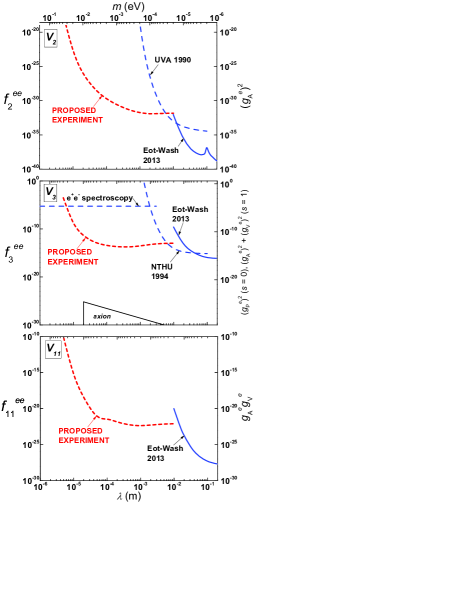
Figure 1: Projected sensitivity of proposed experiment to static spin–spin interactions (Eq. 1), with current limits and theoretical prediction. Interaction strength according to all parameterizations in Table 1 is plotted versus the range $\lambda$ (lower axes) and the mass of an unobserved boson (upper axes). Excluded regions are above the curves. For $V_{2}$, solid curve is the 1 $\sigma$ direct limit on $(g_{A}^{e})^{2}$ Heckel et al. (2013), also expressed as $f_{2}^{ee}$. Dashed curve is the limit from Ritter et al. (1990) re-interpreted in terms of Eq. 1. For $V_{3}$, bold solid curve is the direct limit on $(g_{P}^{e})^{2}$ Heckel et al. (2013), also re-scaled to $f_{3}^{ee}$ in Eq. 1. Dashed curves are the limit from Ni et al. (1994) and the anomaly from Refs. Mills and Bearman (1975)–Hill (2001) re-interpreted in terms of Eq. 1; thin solid curve is the prediction for the axion Moody and Wilczek (1984). For $V_{11}$, solid curve is the direct limit on $g_{A}^{e}g_{V}^{e}$ Heckel et al. (2013), also expressed as $f_{11}^{ee}$.

Fig. 1 also shows the limits on $f_{2}^{ee}$ that can be derived from the spin–polarized torsion pendulum at the University of Virginia Ritter et al. (1990). The spin sources in this experiment consisted of compensated rare earth ferrimagnets, which inspired the proposed experiment in Sec. IV, in the form of powder pressed into high–permeability cylinders and polarized along their symmetry axes. The results of the original experiment are reported in terms of a fraction $\alpha$ of the strength of the (infinite–ranged) magnetic dipole–dipole interaction between electrons:

$$\alpha=(1.6\pm 6.9)\times 10^{-12}.$$ (5)

The test cylinders were oriented side-by-side with their axes parallel, a configuration which strongly suppressed the $\hat{\sigma}\cdot\hat{r}$ terms in the dipole–dipole potential and in which the finite–sized test masses could be approximated by point dipoles up to correction factors of order unity. The curve in Fig. 1 is thus obtained by converting the limit on $\alpha$ to a magnetic dipole–dipole energy and equating it to the expression for $V_{2}$ in Eq. 1, where $r$ is fixed at the 3.4 cm test mass separation reported in Ritter et al. (1990). The long–range limit of the curve corresponds to the result reported for this experiment in Dobrescu and Mocioiu (2006).

Similarly, short–range limits on $f_{3}^{ee}$ can be derived from the experiment by Ni and co-workers at the National Tsing Hua University in Taiwan Ni et al. (1993); Chui and Ni (1993); Ni et al. (1994). This experiment used a SQUID magnetometer to monitor the interaction between spin–polarized test masses (also consisting of compensated rare earth ferrimagnets) and a sample of paramagnetic salt, as the test masses were rotated around the sample at a distance of about 5 cm. The results of this experiment are also reported in terms of the electron magnetic dipole–dipole interaction. The most sensitive result Ni et al. (1994) is: $\alpha_{s}=(1.2\pm 2.0)\times 10^{-14}$. The test mass polarization was oriented either directly toward or away from the salt, maximizing the contribution from the $\hat{\sigma}\cdot\hat{r}$ terms. The curve in Fig. 1 is thus obtained by converting $\alpha_{s}$ to a magnetic dipole–dipole energy and equating it to the expression for $V_{3}$ in Eq. 1, with $r$ fixed at 5 cm. Again, the long–range limit of the curve corresponds to the result reported for this experiment in Dobrescu and Mocioiu (2006).

Below about about 2 mm, stronger limits on $f_{3}^{ee}$ can be inferred from precision measurements of the hyperfine splitting in the ground state of positronium Mills and Bearman (1975); Mills (1983); Ritter et al. (1984). There is currently a $\sim 4\sigma$ difference between these measurements and QED theory Kniehl and Penin (2000); Melnikov and Yelkhovsky (2001); Hill (2001). The horizontal line in the middle plot in Fig. 1 results from equating the energy discrepancy to the expression for $V_{3}$ in Eq. 1, with $r$ fixed at the positronium Bohr radius (0.1 nm). An analogous analysis of the same system has been used to constrain unparticles Liao and Liu (2007).

The $V_{3}$ plot also shows the prediction for the axion (for the case of a spin-0 interaction), for which there exists an explicit relationship between the coupling strength and the range. The value is derived from Moody and Wilczek (1984), and also re-scaled to $f_{3}^{ee}$ according to Table 1. The cutoff at 10 meV is the limit inferred from SN1987a Rosenberg and van Bibber (2000). As noted in Ref. Visinelli and Gondolo , the remaining axion prediction in Fig. 1 (and Fig. 3) is allowed even if the recent BICEP2 measurement of the tensor-to-scalar ratio in the cosmic microwave background Ade et al. is correct, lending additional interest to this part of the parameter space.

Fig. 2 shows the limits on velocity–dependent spin–spin interactions (Eq. 2) in the range of interest. For the case of electrons, these interactions appear to be unconstrained in this range. At $\lambda=1$ km, the lower limit of the range analyzed in Hunter and Ang (2013), the constraints on electron interactions range from $10^{-32}$–$10^{-22}$ for the case of $V_{14}$ and $V_{8}$, to $10^{-7}$–$10^{-1}$ for the case of $V_{16}$ and $V_{15}$, with the remaining interactions constrained at $10^{-17}$–$10^{-12}$.

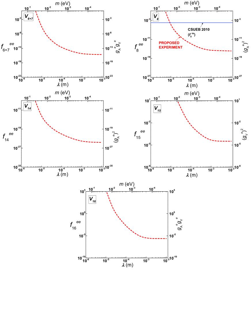
Figure 2: Projected sensitivity of proposed experiment to velocity–dependent spin–spin interactions (Eq. 2). For comparison, the solid curve in the $V_{8}$ plot is an extension of the 2 $\sigma$ limit on $g_{V}^{n}g_{V}^{p}$ for nucleons Kimball et al. (2010), also re-scaled to $f_{8}^{np}$ in Eq. 2.

For comparison, the solid line in the $V_{8}$ plot is the limit calculated for the nucleon coupling $f_{8}^{np}$ by a California State University-East Bay collaboration, based on the analysis of atomic spin exchange interaction cross sections Kimball et al. (2010). The analysis compared the theoretical cross sections, calculated with the usual spin–dependent electromagnetic potentials responsible for spin exchange replaced with potentials of the form in Eqs. 1 and 2, with data from He–Na collisions. The result for $V_{8}$ is reported in Kimball et al. (2010) as a limit on the coupling $g_{A}^{n}g_{A}^{p}$, and has been re-scaled in Fig. 2 according to Table 1, with the additional substitution ${\vec{s}_{2}}=3\hbar\hat{\sigma}_{2}/2$ in the equation for $V_{8}$ to account for the Na nuclei which carried the proton spin. The limit has also been extended beyond the micron range reported in Kimball et al. (2010).

Short–range limits on the interactions in Eq. 3 are shown in Fig. 3. The velocity–dependent interactions $V_{4+5}$ and $V_{12+13}$ appear to be unconstrained for the case of polarized electrons. For comparison, the solid line in the $V_{4+5}$ plot is the limit on the corresponding coupling for polarized nucleons from an experiment at the Paul Scherrer Institute Piegsa and Pignol (2012). This experiment used Ramsey’s technique of separated oscillatory fields to compare the precession rate of polarized cold neutrons in a beam passing in close proximity to a polished copper plate with the precession of neutrons in a reference beam. The result in Piegsa and Pignol (2012), which assumes no coupling to electrons ($f_{\perp}^{ne}=0$) and $f_{\perp}^{np}=f_{\perp}^{nn}\equiv f_{\perp}^{nN}$, is interpreted as a limit on the coupling $(g_{A})^{2}$; the contribution from any $g_{V}$ term is assumed negligible given the much stronger short–range constraints on this parameter from torsion pendulum experiments with unpolarized test masses. The limit in Fig. 3 ($\approx(g_{A})^{2}/4$) has been re-scaled in accordance with these assumptions.

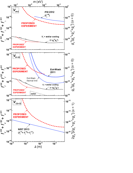
Figure 3: Projected sensitivity of proposed experiment to interactions between polarized and unpolarized particles (Eq. 3), with current limits and theoretical prediction. For comparison, solid curves in the $V_{4+5}$ and $V_{12+13}$ plots are the direct limits (2 $\sigma$ and 1 $\sigma$, respectively) for the case of polarized neutrons Piegsa and Pignol (2012); Yan and Snow (2013). For $V_{9+10}$, the bold solid curve is the 2 $\sigma$ direct limit on $g_{S}^{N}g_{P}^{e}$ Hoedl et al. (2011), also rescaled to $f_{r}^{ee}+f_{r}^{ep}+f_{r}^{en}$ in Eq. 3; bold dashed curve is the projected thermal limit. Thin solid curve is the prediction for the axion Moody and Wilczek (1984). Lower solid curves in the $V_{4+5}$ and $V_{9+10}$ plots are the indirect limits inferred from stellar cooling arguments Raffelt (2012); the additional projected curves show expected improvements from the proposed experiment with unpolarized test masses Long and Price (2003).

Similarly, the solid line in the $V_{12+13}$ plot is the limit on the corresponding coupling for polarized neutrons derived from the neutron spin rotation experiment at NIST Yan and Snow (2013). This experiment is designed to be sensitive to the rotation $\phi$ of the polarization of a transversely polarized beam of neutrons passing through a liquid ⁴He target. The rotation $\phi$ arises from a $P$–violating $\hat{\sigma}\cdot\hat{p}$ term in the forward scattering cross section, whether induced by an interaction such as $V_{12+13}$ or the Standard Model weak interaction to which the experiment is ultimately designed to be sensitive. The analysis in Yan and Snow (2013) uses the result on $\phi$, currently an upper limit, to constrain $V_{12+13}$. The limit is reported in terms of $g_{V}g_{A}^{n}$, where $g_{V}$ contains a factor $Z=2$ for ⁴He. Equating the expression for $V_{12+13}$ in Yan and Snow (2013) to Eq. 3 for polarized neutrons, and using $Z=2$, $A=4$ yields the result ($f_{v}^{ne}+f_{v}^{np}+f_{v}^{nn}=g_{V}g_{A}^{n}$) in Fig. 3.

The best limit on the $V_{9+10}$ interaction for electrons is derived from the Axion-Like Particle (ALP) torsion pendulum in the Eot-Wash group, which consists of a thin silicon wafer suspended between the two halves of a split toroidal magnet Hoedl et al. (2011). The magnet provides the polarized electrons, and the wafer a source of unpolarized nucleons highly insensitive to the classical magnetic field present. The limit in Hoedl et al. (2011) is reported in terms of $g_{S}^{N}g_{P}^{e}$, where $g_{S}^{N}\equiv g_{S}^{p}=g_{S}^{n}=g_{S}^{a}/A$ and it is assumed $g_{S}^{e}=0$. Since the unpolarized mass consists of silicon, the limits in Fig. 3 ($f_{r}^{ee}+f_{r}^{ep}+f_{r}^{en}\approx 2g_{S}^{N}g_{P}^{e}$) are scaled according to Table 1 with these assumptions, where the dashed line is the projected thermal limit from Hoedl et al. (2011). The same scaling applies to the prediction for the axion, shown in the $V_{9+10}$ plot for the case of an $s=0$ interaction. The prediction is again from Moody and Wilczek (1984), updated to account for the value of $\theta_{QCD}$ Crewther et al. (1979); *cre80 inferred from the current best limit on the electric dipole moment of the neutron Baker et al. (2006).

Finally, the $V_{9+10}$ plot in Fig. 3 also shows the indirect limits derived from a combination of data from laboratory experiments and astrophysical arguments Raffelt (2012). These are limits on the coupling $g_{S}^{N}g_{P}^{e}$, i.e., for the case of an $s=0$ interaction, in which the constraints on $g_{S}^{N}$ come from short–range gravity experiments with unpolarized test masses Kapner et al. (2007); Geraci et al. (2008); Sushkov et al. (2011), and the limit on $g_{P}^{e}$ comes from stellar cooling. They have been scaled by the same factor in Fig. 3 as the limit in Hoedl et al. (2011) to maintain consistency with the results in Raffelt (2012). As noted in Dobrescu and Mocioiu (2006), analogous constraints on $g_{S}^{N}g_{S}^{e}$ can be inferred by combining the same results for $g_{S}^{N}$ with the stellar cooling limit on $g_{S}^{e}$. Using $g_{S}^{e}\leq 1.3\times 10^{-14}$ from Raffelt (2012), the resulting limits are shown in the $V_{4+5}$ plot for the case of an $s=0$ interaction.

IV Short–Range Experiment

The experiment is illustrated in Fig. 4. It has been used previously to set limits on mass–coupled forces in the range of interest Long et al. (2003) and a more sensitive version of it is currently fully operational. The experimental test masses consist of 1 kHz, planar mechanical oscillators with a thin shield between them to suppress backgrounds. The planar geometry is especially efficient for concentrating as much mass as possible at the range of interest. It is nominally null with respect to $1/r^{2}$ forces and thus effective in suppressing Newtonian backgrounds. The (active) source mass is driven at a resonance frequency of the (passive) detector mass to maximize the signal. For the mass–coupled force search the test masses are made from tungsten, which has a density of about 19 g/cm³. Resonant operation places a heavy burden on vibration isolation. The 1 kHz operational frequency is chosen since in this frequency range it is possible to construct a simple, passive vibration isolation system with high dimensional stability Chan et al. (1999), permitting the test mass surfaces to be maintained within a few microns of each other for indefinite periods.

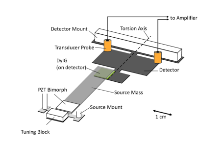
Figure 4: (adapted from Long et al. (2003) and Yan et al. (2014)) Basic test mass geometry of the proposed experiment. In the particular configuration, a thin sample of spin-polarized material (here DyIG) covers half of the small forward rectangle of the detector mass. In other configurations, a similar sample is attached to the underside of the forward part of the source mass. The thin, stiff, conducting shield between the test masses is not shown.

The source mass is a nodally–mounted cantilever driven by a piezoelectric wafer attached in a region of high modal curvature. The detector is a planar double–torsional oscillator originally developed for cryogenic condensed matter physics experiments Kleiman et al. (1985); Klitsner and Pohl (1986). It consists of 2 coplanar rectangles, joined along their central axes by a short segment. The resonant mode of interest is the first anti-symmetric torsion mode, in which the rectangles counter-rotate about the axis defined by the segment. This mode is distinguished by a high mechanical quality factor ($Q$), important for increasing sensitivity and suppressing thermal noise. To eliminate backgrounds mediated by electrostatic, residual gas, and possible Casimir effects, it is essential to place a stiff conducting shield between the test masses. The previous experiment Long et al. (2003) used a 60 micron thick gold-coated sapphire plate clamped at two opposite ends, which was completely effective at suppressing these backgrounds. The existing experiment uses a thinner shield made from a stretched copper membrane. Detector oscillations are read out with a capacitive transducer coupled to a differential amplifier, which is sufficiently sensitive to monitor the detector thermal motion Yan et al. (2014).

To make the experiment sensitive to spin–dependent interactions, samples of spin–polarized materials can be attached to the test masses (Fig. 4). The principal challenges will be to fabricate such samples with the necessary thin planar geometry while retaining the polarization, and to control the extra backgrounds due to residual magnetic forces that cannot be eliminated. For the spin–polarized material, compensated ferrimagnets are an intriguing possibility. These materials contain at least two magnetic sublattices in which the magnetic moments are oppositely aligned. The contributions of each sub-lattice to the magnetization of a sample depend on temperature in such a way that there is a “compensation” temperature ($T_{c}$) at which their magnitudes are equal and thus cancel. For materials in which the contributions to the magnetism of each sub-lattice from spin and orbital motion of the electrons are different, at the compensation temperature there is a net spin.

The effect on the detector $Q$ of attaching a polarized sample is not known. However, silicon test mass prototypes, which are particularly attractive as low–susceptibility substrates for the spin–dependent experiments, have been measured to have $Q$s as high as $2\times 10^{6}$ between 77 K and room temperature. For the purpose of the sensitivity estimates, a conservative value of $Q=10000$ is assumed.

To locate the compensation temperature (assuming $T_{c}<295$ K), the experiment can be cooled radiatively with a high-emissivity shield surrounding the central apparatus. The test mass temperatures can be further adjusted with thermoelectric elements. The absolute magnetization of the samples away from the compensation temperature, from which the degree of spin–polarization can be deduced, can be measured using external coils to produce a resonant, calibrated, quasi–uniform magnetic gradient to drive the test masses.

Test mass development

One candidate material for the polarized test masses, Dy₆Fe₂₃, has been used in previous experiments Ritter et al. (1990); Ni et al. (1993); Chui and Ni (1993); Ni et al. (1994); Hou et al. (2003). Dy₆Fe₂₃ is a ferrimagnet with a net spin and a compensation temperature of about 250 K. The Dy-Fe system exhibits several phases, however, and synthesis of the pure 6-23 phase can be problematic van der Goot and Buschow (1970); Herbst and Croat (1984). It oxidizes readily and the samples in the reported experiments are encapsulated, making it less attractive for fabrication of small samples that must be kept in close proximity. This work investigates the rare earth iron garnets, in particular dysprosium iron garnet (DyIG), Dy${}_{3}^{3+}$Fe${}_{2}^{3+}$Fe${}_{3}^{3+}$O₁₂, as a possible alternative. The garnets are chemically stable and can be produced in the lab with little difficulty.

IV.0.1 Molecular field model

DyIG is a ferrimagnet in which three sublattices contribute to the magnetization. The Dy³⁺ ions occupy dodecahedral sites (commonly denoted $c$) in the garnet lattice, the Fe³⁺ octahedral sites (denoted $a$) and tetrahedral sites (denoted $d$) Dionne (2009). The Dy³⁺ moments are nominally aligned with the octahedral ion moments and anti-aligned with the tetrahedral moments. The total magnetization per molecule $M$ at a particular temperature is thus:

$$M=M_{c}+M_{a}-M_{d}.$$ (6)

Following Dionne (2009), the contribution of each sublattice can be calculated in a molecular field model. The temperature–dependent sublattice moments are given by:

$$M_{c}(T) = M_{c}(0)B_{J_{c}}(x_{c})$$

$$M_{a}(T) = M_{a}(0)B_{J_{a}}(x_{a})$$

$$M_{d}(T) = M_{d}(0)B_{J_{d}}(x_{d}),$$ (7)

where $M_{i}(0)$ are the 0 K moments and the $B_{J_{i}}(x_{i})$ are the Brillouin functions for sublattice $i$. For pure DyIG (that is, no substitution of the ions on any sublattice) the 0 K moments are:

$$M_{c}(0) = 3g_{c}\mu_{B}J_{c}N_{A}$$

$$M_{a}(0) = 2g_{a}\mu_{B}J_{a}N_{A}$$

$$M_{d}(0) = 3g_{d}\mu_{B}J_{d}N_{A}.$$ (8)

Here, $\mu_{B}$ is the Bohr magneton in units of erg/Gauss and a factor of Avogadro’s number $N_{A}$ is included to convert $M$ to units of $\mu_{B}$/molecule. The coefficients in Eq. 8 represent the relative numbers of $c$, $a$, and $d$ sites in the garnet molecule Dionne (1970). The terms $g_{i}$ and $J_{i}$ are the Lande g-factor and total angular momentum of the ion on sublattice $i$.

The Boltzmann energy ratios $x_{i}$ in Eq. 7 are given by:

$$x_{c} = \frac{g_{c}J_{c}\mu_{B}}{k_{B}T}[N_{cc}M_{c}+N_{ac}M_{a}+N_{cd}M_{d}]$$

$$x_{a} = \frac{g_{a}J_{a}\mu_{B}}{k_{B}T}[N_{ac}M_{c}+N_{aa}M_{a}+N_{ad}M_{d}]$$

$$x_{d} = \frac{g_{d}J_{d}\mu_{B}}{k_{B}T}[N_{cd}M_{c}+N_{ad}M_{a}+N_{dd}M_{d}],$$ (9)

where the $N_{ij}$ are the molecular field coefficients. Here, the exchange fields (terms in brackets) are expressed in Gauss so that the $N_{ij}$ are in units of mol/cm³. With appropriate values of $g_{i}$ and $J_{i}$, Eqs. 7 and 9 are solved iteratively for the three lattices simultaneously. The $N_{ij}$ are adjusted by trial and error to reproduce the data on magnetization vs. temperature for pure DyIG crystals.

Fig. 5 shows the result of the calculations of magnetization vs. temperature using $N_{ac}=-4.0$ mol/cm³, $N_{dc}=6.0$ mol/cm³ Dionne (2009), $N_{cc}=0$ Dionne (1976), and $N_{aa}=-65.0$ mol/cm³, $N_{ad}=97.0$ mol/cm³, and $N_{dd}=-30.4$ mol/cm³ Dionne (1971). The calculation predicts $T_{c}=226$ K. At $T_{c}$, the three Dy³⁺ ions contribute 4.1 $\mu_{B}$ to the magnetic moment of the DyIG molecule. The two Fe³⁺ on the $a$ sublattice contribute 9.5 $\mu_{B}$, and the three Fe³⁺ on the $d$ sublattice contribute -13.6 $\mu_{B}$. The (absolute value of the) total magnetization curve displays good agreement with data from measurements on single crystal spherical samples Geller et al. (1965).

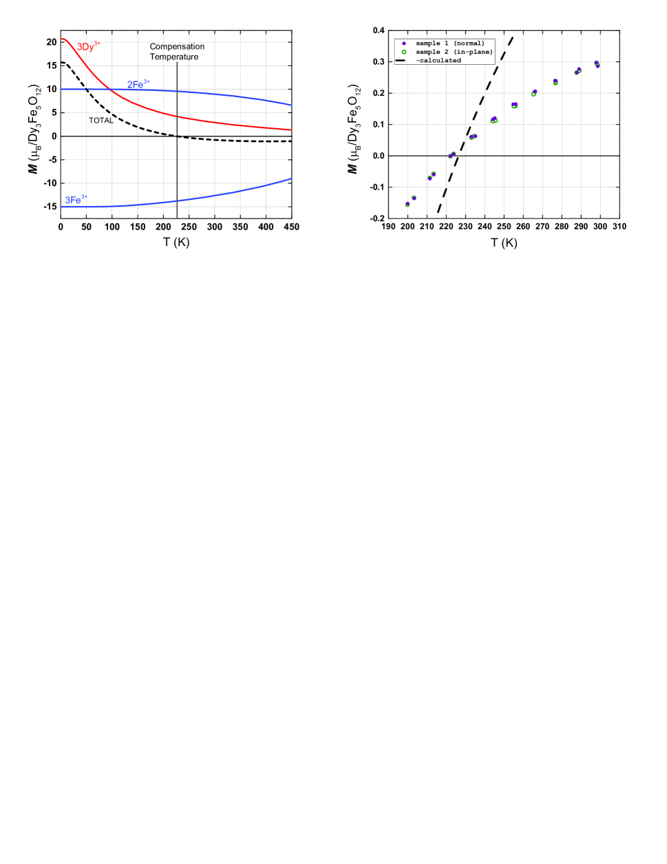
Figure 5: Left: Magnetization of DyIG versus temperature, from the results of the molecular field calculation described in the text. Contributions from the ions on each sublattice are shown (bold curves), together with the sum (dashed curve). Right: Magnetization vs temperature of the particular DyIG samples fabricated for the proposed experiment. At each temperature investigated, there are two data points for each sample, one taken as the sample is cooled from 295 K, the other as the sample warmed from 200 K. The dashed line is the (negative of the) calculated total magnetization in the left-hand plot, for comparison with the slope of the experimental curves at $T{c}$.

An analogous calculation for terbium iron garnet (TbIG), using the appropriate $N_{ij}$ from the same references, predicts $T_{c}=266$ K. The Tb³⁺ ions contribute 4.0 $\mu_{B}$ to the total moment at $T_{c}$.

The Fe³⁺ ions on the $a$ and $d$ sublattices have spin $S=5/2$ and orbital angular momentum $L=0$. Consequently, $J_{a}=J_{d}=5/2$ and $g_{a}=g_{d}=2$ for the calculation in Fig. 5. It should be noted that, for ions in the $3d^{n}$ series bonded in an anion lattice such as garnet, the $3d$ shells are exposed to the electrostatic fields of the lattice so that $L$ is uncoupled from $S$, the process known as quenching. A consequence is that $S$ is the principal source of the magnetic moment and $g=2$ a good approximation for most ions in this series. The same effect has implications for the correct values of $J_{c}$ and $g_{c}$.

The configuration of the Dy³⁺ ion is $4f^{9}$. In contrast to the Fe³⁺ ions, the magnetically active $4f$ electrons in the rare earth are shielded by the electrons in the full $5s$ and $5p$ outer shells, thus they are not expected to be affected by the lattice fields. The free Dy³⁺ ion has $S_{c}=5/2$ and $L_{c}=5$, for $J_{c}=15/2$ and $g_{c}=4/3$. However, these are not the values used in the calculation in Fig. 5. To reproduce the data, the effective value of $J_{c}$ is reduced, the process known as canting. Ref. Dionne (2009) discusses two possible models.

In the first or semiclassical model, the $J_{c}$ vector is tilted with respect to the direction defined by the spins of the $d$ lattice. Thus a projection $J_{c}^{\prime}=5.25$ is used in Eqs. 7–9, together with $g_{c}=4/3$. In the second model, $L_{c}$ is partially quenched in the lattice field, leading to an actual reduction in $J_{c}$. Following the notation in Dionne (2009), the quenching factor is $\gamma=0.38$, so that $L_{c}^{\prime\prime}=\gamma L_{c}=1.9$, $J_{c}^{\prime\prime}=L_{c}^{\prime\prime}+S_{c}=4.4$, and

$$g_{c}^{\prime\prime}=1+\frac{J_{c}^{\prime\prime}(J_{c}^{\prime\prime}+1)+S_{c}(S_{c}+1)-L_{c}^{\prime\prime}(L_{c}^{\prime\prime}+1)}{2J_{c}^{\prime\prime}(J_{c}^{\prime\prime}+1)}=1.57$$

Either model produces the curves in Fig. 5. However, as explained in Dionne (2009), the latter model with partially quenched $L_{c}$ is more consistent with the results of measurements in fields applied along the direction of the crystal fields. It is also more conservative for the purpose of estimating the spin excess of DyIG at $T_{c}$, and thus is adopted here.

The spin contribution of the ions on the $i$th sublattice to the total magnetic moment can be deduced from the spin g-factors, $g_{s_{i}}$. For the Fe³⁺ ions, which have $L=0$ and $g_{s}=g=2$, all of the contribution is due to spin. For the Dy³⁺ ions in the lattice,

$$g_{s}^{\prime\prime}=1+\frac{S_{c}(S_{c}+1)-L_{c}^{\prime\prime}(L_{c}^{\prime\prime}+1)}{J_{c}^{\prime\prime}(J_{c}^{\prime\prime}+1)}=1.14.$$

In this case, 73% of the magnetic moment is due to spin and 27% is due to the orbital motion of the electrons. Thus, at $T_{c}$, $\mu_{s_{c}}=3.1$ $\mu_{B}$ and the total spin excess per molecule (in units of $\hbar$) is:

$$S_{T_{c}}=\frac{|\mu_{s_{T}}|}{2\mu_{B}}=\frac{|3.1+9.6-13.8|}{2}=0.6.$$ (10)

The analogous calculation for TbIG ($L_{c}=S_{c}=3,\gamma=0.32$ Dionne (2009)) yields $S_{T_{c}}=0.3$. Thus while TbIG may be more attractive for its higher $T_{c}$, the spin excess is reduced by a factor of 2.

IV.0.2 Synthesis and properties

Samples of DyIG practically sized for use in the proposed experiment are synthesized via the chemical process described in Gesselbracht et al. (1994). The material is precipitated from a mixed metal hydroxide precursor solution and dried in an oven (air atmosphere) at 393 K for 12 hr. It is then hand-ground to fine powder, and pressed (force = 10 kN) into 3.2 mm diameter pellets using a precision die mounted in a hydraulic press. The pellets are then fired in the oven at 1173 K for 18 hr. Repetition of the grinding, pressing, and firing steps has been shown to increase purity Gesselbracht et al. (1994); Uemura et al. (2008); these steps were repeated twice for the pellets in the present study. Two such samples were fabricated, sample 1 with thickness 0.84 mm and density 3.4 g/cm³, sample 2 with thickness 0.97 mm and density 3.5 g/cm³.

The sample magnetic properties were measured with a SQUID magnetometer (Quantum Design MPMS–XL) calibrated with a palladium standard. Both samples were magnetized to saturation at room temperature in an applied field of 2 T, then the applied field was ramped to zero. Sample 1 was magnetized in the direction normal to the plane of the pellet along the symmetry axis, sample 2 was magnetized in-plane (both polarizations are necessary for sensitivity to all potentials in Eqs. 1–3, as explained in Sec. V).

The remnant magnetization of the samples was then measured as the temperature was reduced below the anticipated $T_{c}$, then raised back to room temperature. Results are shown in Fig. 5. For both samples, the magnetization drops to zero at a $T_{c}$ near 223 K, reverses below, then recovers to the initial magnetization at room temperature. Subsequent measurements show this behavior to be repeatable upon multiple excursions through $T_{c}$, and when the samples are held at $T_{c}$ for several hours. Results are very similar for the two polarizations, indicating little if any extra demagnetization in the case of normal polarization.

The spin density of each sample at $T_{c}$ (assuming the density of the pellets to be uniform) is given by:

$$n_{s}=\frac{N_{A}\rho}{A}S_{T_{c}},$$ (11)

where $\rho$ is the mass density of the sample and $A=958.5$ g/mol is the atomic weight of DyIG. Following Ritter et al. (1990), an additional correction factor, equal to the ratio of the slope of the calculated magnetization curve to the measured curves at $T_{c}$, is applied in order to account for incomplete magnetization of the flat, polycrystalline samples used. This ratio is 0.36, resulting in spin densities of $n_{s}=4.0\times 10^{20}$ $\hbar$/cm³ for sample 1 and $n_{s}=4.1\times 10^{20}$ $\hbar$/cm³ for sample 2.

V Projected sensitivities

The sensitivity of the experiment is based on the expectation that essentially all experimental backgrounds can be suppressed below the detector thermal noise and amplifier noise. This represents an ultimate practical sensitivity; results with reduced but competitive sensitivity in the presence of other backgrounds are expected to be realized sooner.

Experimental signals are estimated by converting Eqs. 1–3 to forces and integrating them numerically over the test mass geometry, assuming values of 1 for the coupling constants. For simplicity, it is assumed that each of the interactions in Eqs. 1–3 acts independently, as is the case for the limits in Sec. III. (Additional limits on the interactions in Eq. 1 are presented in Heckel et al. (2013), in which this assumption is relaxed.) The thermal noise force due to dissipation in the detector is found from the mechanical Nyquist formula,

$$F_{T}=\sqrt{\frac{4k_{B}Tm\omega_{0}}{Q\tau}},$$ (12)

where $k_{B}$ is Boltzmann’s constant, $T$ is the temperature, $m$ is the mass of the detector oscillator, $\omega_{0}$ is the resonance frequency, $Q$ is the mechanical quality factor, and $\tau$ is the experimental integration time. The ratio of this force to the result of the integration of Eqs. 1–3 at each value of $\lambda$ used (that is, a signal–to–noise ratio of 1) yields the sensitivity curves for the coupling constants. Since the experiment is sensitive to changes in the signal as the test mass separation is varied, the integration models the sinusoidal modulation of the source mass and calculates the Fourier amplitudes of the integrated signal. In the thermal noise limit, the amplitude of the oscillations of the detector is of order $\sqrt{k_{B}T/(m\omega_{0}^{2})}\sim 1$ pm (Table 2), thus the relative velocity term $\vec{v}$ in Eqs. 1–3 is very well approximated by the source velocity.

To maximize sensitivity at short range, a small but reasonable minimum test mass gap (that is, distance of closest approach) is assumed. This is fixed at 120 $\mu$m. This allows for a 100 $\mu$m thick shield between the test masses (40 $\mu$m thicker than the shield used successfully in previous experiments Long et al. (2003), thus reserving space for additional magnetic shielding if needed). For each value of $\lambda$ investigated, the source mass amplitude is optimized for maximum signal. For the static interactions in Eqs. 1–3, this results in values of order $\lambda$. For all $\lambda$ above 1 mm, an amplitude of 1 mm is used, which is taken to represent a practical maximum with the piezoelectric drive technique. The optimization is the same for the velocity-dependent interactions. The exceptions are $V_{8}$ and $V_{16}$, which, on account of the $v^{2}$ dependence, increase monotonically with source amplitude at any $\lambda$ over the range of interest. For these interactions, the maximum practical source amplitude of 1 mm is used at each value of $\lambda$.

Sensitivity to all interactions in Eqs. 1–3 is possible in principle with simple modifications to the test mass geometry and polarization. The different configurations are illustrated in Fig. 6. For the purposes of the sensitivity calculations, pure vertical translation of the source mass (along the $z$-axis in Fig. 6) is assumed, with instantaneous velocity $v$. This is a good approximation for the planar geometry but there will be small corrections for the actual mode shape of a practical source mass. The six configurations include four in which the spin–polarized material covers only half of the detector mass and the source mass is positioned over that half, so that the resulting force is optimized to excite the sensitive torsional mode of the detector:

• Detector and source polarization in–plane and parallel. Presumably the easiest configuration to attain for spin–spin interactions and sensitive to potentials proportional to $\hat{\sigma}_{1}\cdot\hat{\sigma}_{2}$.

• Polarization normal to the test mass planes and parallel to $\vec{v}$, for optimum sensitivity to $\hat{\sigma}_{1}\cdot\hat{\sigma}_{2}$ and spin–spin interactions proportional to $\hat{\sigma}\cdot\hat{r}$ and $\hat{\sigma}\cdot\vec{v}$.

• Polarization normal (detector only) and parallel to $\vec{v}$, for optimum sensitivity to spin–mass interactions proportional to $\hat{\sigma}\cdot\hat{r}$ and $\hat{\sigma}\cdot\vec{v}$.

• Polarization in–plane and crossed, for sensitivity to spin–spin interactions proportional to $(\hat{\sigma}_{1}\times\hat{\sigma}_{2})\cdot\hat{r}$ and $(\hat{\sigma}_{1}\times\hat{\sigma}_{2})\cdot\vec{v}$.

In the two remaining configurations, the polarized material covers the entire detector surface and the source is centered over the detector, for sensitivity to interactions proportional to $\vec{v}\times\hat{r}$. The $\vec{v}\times\hat{r}$ term averages to zero over the surface of the detector in this configuration, however, the associated vector field has the profile of a vortex centered in the detector plane. Thus, for $\hat{\sigma}_{1}$ parallel to the detector torsion axis, a force proportional to $\hat{\sigma}_{1}\cdot(\vec{v}\times\hat{r})$, while averaging to zero over the entire detector plane, averages to a non-zero value on one side of the torsion axis and the negative of this value on the other, efficiently driving the torsional mode of interest:

• Polarization in–plane, parallel to detector torsion axis, for sensitivity to spin–mass interactions proportional to $\hat{\sigma}\cdot(\vec{v}\times\hat{r})$.

• Polarization mixed, with one parallel to detector torsion axis, for sensitivity to spin–spin interactions proportional to $[\hat{\sigma}_{1,2}\cdot(\vec{v}\times\hat{r})](\hat{\sigma}_{2,1}\cdot\hat{r})$ and $[\hat{\sigma}_{1,2}\cdot(\vec{v}\times\hat{r})](\hat{\sigma}_{2,1}\cdot\vec{v})$.

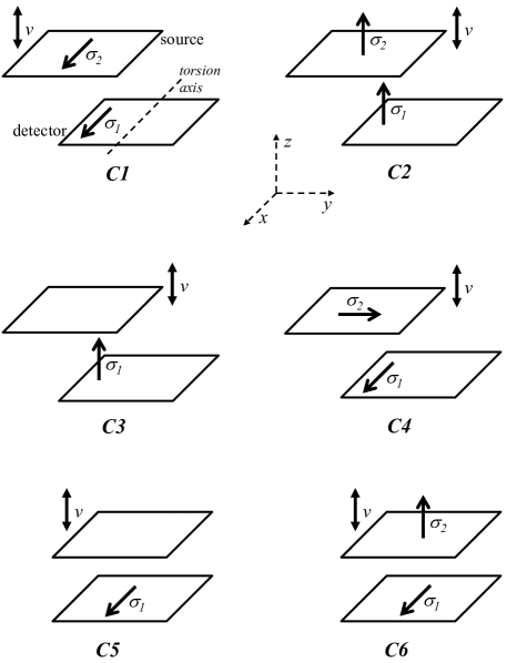
Figure 6: Test mass and spin polarization configurations used to search for interactions $V_{2}$–$V_{16}$ as assumed in the sensitivity calculations. Here, $\sigma_{1}$ is the net polarization direction of the spins in the detector mass and $\sigma_{2}$ in the source mass. The relative velocity of the spins in each test mass is strongly dominated by the velocity of the source, $v$. The detector torsion axis is along $x$. $C1$: polarization in–plane, parallel ($V_{2}$, $V_{3}$). $C2$: polarization normal ($V_{2}$, $V_{3}$, $V_{6+7}$, $V_{8}$). $C3$: polarization normal, detector only ($V_{9+10}$, $V_{12+13}$). $C4$: polarization in–plane, crossed ($V_{11}$, $V_{14}$). $C5$: polarization in–plane, detector only ($V_{4+5}$). $C6$: polarization mixed ($V_{15}$, $V_{16}$). Note that in $C_{1}$–$C_{4}$, the source subtends half the detector area and the polarized material $\sigma_{1}$ covers only the detector area subtended. In $C_{5}$ and $C_{6}$, the source mass is centered over the detector and $\sigma_{1}$ covers the entire detector area.

Parameters used in the sensitivity calculations are listed in Table. 2.

Table 2: Test mass geometry and other properties used in sensitivity calculations. For searches in which the source is centered over the detector ($V_{4+5},V_{15},V_{16}$), the active detector area is 58 mm². For interactions $V_{4+5},V_{9+10}$, and $V_{12+13}$, the source is unpolarized and consists of silicon (density 2.3 g/cm³).

Parameter	value
Active detector area	29 mm2
Active source mass area	36 mm2
Test mass thickness	1 mm
Test mass density	3.5 g/cm3 (DyIG)
Test mass spin density	$4\times 10^{20}/$cm3
Minimum source-detector gap	120 $\mu$m
Signal frequency	1 kHz
Detector quality factor	$1\times 10^{4}$
Temperature	225 K
Integration time	200 hr

Results for sensitivity to the static spin–spin interactions (Eq. 1) are shown in Fig. 1. The sensitivity to the $V_{2}$ interaction is comparable to the Eot–Wash and UVA experiments in the range near 1 cm, but many orders more so only a few millimeters below on the account of the small test mass separation.

The projected limit on $V_{2}$ is the most sensitive relative to the others, by at least 4 orders of magnitude, in the range of interest. The remaining projections can be roughly grouped into three regions of successively decreasing sensitivity, determined by the number of additional factors of $1/r$ or $v/c$ in the expressions for the corresponding interactions (Eqs. 1-3) relative to $V_{2}$.

The sensitivity to the $V_{3}$ dipole-dipole interaction is about eight orders of magnitude greater than the limit inferred from positronium spectroscopy at 20 $\mu$m. Results for sensitivity to the velocity–dependent spin–spin interactions (Eq. 2) are shown in Fig. 2. The proposed technique would appear to have unique sensitivity in this range.

Results for sensitivity to interactions between polarized electrons and unpolarized atoms (Eq. 3) are shown in Fig. 3. The sensitivity to the $V_{9+10}$ monopole–dipole interaction is about eight orders of magnitude greater than the current experimental limits at 20 $\mu$m. The lower dashed curves in the $V_{4+5}$ and $V_{9+10}$ plots are the projected limit on $g_{S}^{N}g_{S}^{e}$ and $g_{S}^{N}g_{P}^{e}$, respectively, using the value for $g_{S}^{e}$ and $g_{P}^{e}$ from stellar cooling Raffelt (2012) and the projected limit on $g_{S}^{N}$ from the version of the proposed experiment using dense, unpolarized test masses Long and Price (2003).