Gauge properties of the guiding center variational symplectic integrator

Abstract

Variational symplectic algorithms have recently been developed for carrying out long-time simulation of charged particles in magnetic fieldsQin and Guan (2008); Qin et al. (2009); Li et al. (2011). As a direct consequence of their derivation from a discrete variational principle, these algorithms have very good long-time energy conservation, as well as exactly preserving discrete momenta. We present stability results for these algorithms, focusing on understanding how explicit variational integrators can be designed for this type of system. It is found that for explicit algorithms an instability arises because the discrete symplectic structure does not become the continuous structure in the $t\rightarrow 0$ limit. We examine how a generalized gauge transformation can be used to put the Lagrangian in the "antisymmetric discretization gauge," in which the discrete symplectic structure has the correct form, thus eliminating the numerical instability. Finally, it is noted that the variational guiding center algorithms are not electromagnetically gauge invariant. By designing a model discrete Lagrangian, we show that the algorithms are approximately gauge invariant as long as $\bm{A}$ and $\phi$ are relatively smooth. A gauge invariant discrete Lagrangian is very important in a variational particle-in-cell algorithm where it ensures current continuity and preservation of Gauss’s lawSquire et al. .

In many applications involving magnetized plasmas, it is necessary to numerically integrate particle dynamics over long time scales. A crucial associated tool is the guiding center description Littlejohn (1983), which averages over fast gryomotion, allowing a dramatic decrease in necessary computational resources through the use of much longer time steps Lin et al. (1998); Chen and Parker (2003); Cohen et al. (1980). Traditional integration routines (for instance Runga-Kutta) for the guiding center equations, while much more efficient than integration of the full Lorentz force equations, can perform badly over very long simulation times. To mitigate these problems and improve confidence in simulation results, variational integrators for the guiding center equations have recently been presented in Refs. Qin and Guan, 2008; Qin et al., 2009; Li et al., 2011. Based on a discretization of the variational principle rather than the equations of motion Veselov (1988), these algorithms exactly conserve a symplectic structure Channell and Scovel (1990); Candy and Rozmus (1991); Feng (1986); Yoshida (1990). As a consequenceMarsden and West (2001); Channell and Scovel (1990); Reich (1999); Veselov (1988) they exhibit very good long time conservation properties, and numerical solutions stay close to exact dynamics, even at large time-step. In addition, a discrete Noether’s theorem implies that exact numerical conservation laws arise from symmetries of the system, for instance momentum conservation due to translational invariance.

The basic idea behind variational integrators is simple and represents a departure from the usual approach of deriving continuous equations of motion from a continuous Lagrangian and then discretizing these differential equations. Instead, the Lagrangian itself is discretized and an integrator is derived from this discrete variational principle Marsden and West (2001). In this process, there is of course some freedom in the chosen discretization of the Lagrangian. For example, $\bm{x}\left(t\right)$ could be discretized as $\bm{x}_{k}$, or as $\frac{1}{2}\left(\bm{x}_{k}+\bm{x}_{k+1}\right)$. In this paper we investigate a different type of freedom that has previously not been studied (to our knowledge) – the freedom to gauge transform the continuous Lagrangian. It is well known that a generalized gauge transformation, $L\rightarrow L+\frac{d}{dt}S$, does not change the continuous Euler-Lagrange equations of motion. Nevertheless, the discrete Euler-Lagrange equations derived from a discretization of $L$ are in general not the same as those from a discretization of $L+\frac{d}{dt}S$. This article presents the results of a systematic investigation of the effects of these gauge transformations on the properties of the variational symplectic guiding center algorithms. In particular, we find that the choice of gauge can profoundly alter the algorithms’ stability properties. These results are intended to be a guide for future users of the guiding center algorithms, as well as variational integrators for systems with Lagrangians of a similar form – such as the magnetic field line Lagrangian Cary and Littlejohn (1983) or point vortices Rowley and Marsden (2002).

The lowest order non-canonical Lagrangian for the guiding center system, given by Grebogi and Littlejohn Grebogi and Littlejohn (1984); Littlejohn (1983), is

$$L=\left[\bm{A}\left(\bm{x}\right)+U\bm{b}\left(\bm{x}\right)\right]\cdot\dot{\bm{x}}+\mu\dot{\Theta}-\left[\phi\left(\bm{x}\right)+\Gamma\left(\bm{x},U\right)\right].$$ (1)

Here $\bm{x}$ is the guiding center position, $U=\gamma u$ is the relativistic momentum parallel to the magnetic field (with $\gamma$ the relativistic mass factor), $\mu$ is the conserved magnetic moment, $\Theta$ is the gyrophase, $\bm{b}\left(\bm{x}\right)$ is the magnetic field unit vector, $\bm{A}\left(\bm{x}\right)$ is the magnetic vector potential, $\phi\left(\bm{x}\right)$ is the electric potential and $\Gamma\left(\bm{x},U\right)=\sqrt{1+U^{2}+2\mu B\left(\bm{x}\right)}.$ Note $\bm{A}$ is normalized by $c/e$, $\Gamma$ by $1/mc^{2}$ and $\phi$ by $1/e$. In the non-relativistic limit, $U$ becomes $u$ (parallel velocity) and $\Gamma$ becomes $1+u^{2}/2+\mu B\left(\bm{x}\right)$. Since only the time derivative of the gyrophase ($\Theta$) appears in Eq. (1), the equation of motion for $\mu$ is simply $\mu\left(t\right)=\mu\left(0\right)$ and we ignore this term in the Lagrangian for the remainer of the article. Continuous particle guiding center equations of motion are derived as usual from Eq. (1) with the Euler-Lagrange equations.

The variational symplectic guiding center algorithms in Refs. Li et al., 2011; Qin and Guan, 2008; Qin et al., 2009 are derived from discretizations of Eq. (1). We give a brief overview of this process for clarity. For the algorithm of Refs. Qin and Guan, 2008; Qin et al., 2009 the (non-relativistic) discrete Lagrangian is chosen to be,

$$L_{d}\left(k,k+1\right)= \frac{1}{2}\left[\bm{A}^{\dagger}\left(\bm{x}_{k}\right)+\bm{A}^{\dagger}\left(\bm{x}_{k+1}\right)\right]\cdot\frac{\left(\bm{x}_{k+1}-\bm{x}_{k}\right)}{h}$$

$$- \left[\frac{u_{k}u_{k+1}}{2}+\mu B\left(\bm{x}_{k}\right)+\phi\left(\bm{x}_{k}\right)\right],$$ (2)

where $\bm{A}^{\dagger}\left(\bm{x}\right)\equiv\bm{A}\left(\bm{x}\right)+u\,\bm{b}\left(\bm{x}\right)$. Eq. (2) is a direct approximation of $\frac{1}{h}\int_{t_{k}}^{t_{k+1}}dt\,L\left(\bm{x},\dot{\bm{x}},U,\dot{U}\right)$. Requiring stationarity of the discrete action $\mathcal{A}_{d}=\sum_{k}hL_{d}$ under arbitrary variations $\left(\delta\bm{x}_{k},\,\delta u_{k}\right)$ $\left(0<k<N\right)$, leads to the discrete update equations for the system,

$$\frac{1}{2h} A_{i,j}^{\dagger}\left(\bm{x}_{k}\right)\left(x_{k+1}^{i}-x_{k-1}^{i}\right)-\frac{1}{2h}\left[A_{j}^{\dagger}\left(\bm{x}_{k+1}\right)-A_{j}^{\dagger}\left(\bm{x}_{k-1}\right)\right]$$

$$=\,\mu B_{,j}\left(\bm{x}_{k}\right)+\phi_{,j}\left(\bm{x}_{k}\right)\qquad\left(j=1,\,2,\,3\right),$$ (3)

$$\frac{1}{2h} b_{i}\left(\bm{x}_{k}\right)\left(x_{k+1}^{i}-x_{k-1}^{i}\right)=\frac{1}{2}\left(u_{k+1}+u_{k-1}\right).$$ (4)

These equations are solved implicitly to integrate particle motion through phase space. For the purposes of this article, the discretization of Eq. (2), $\bm{A}^{\dagger}\left(\bm{x}\right)\rightarrow\frac{1}{2}\left[\bm{A}^{\dagger}\left(\bm{x}_{k}\right)+\bm{A}^{\dagger}\left(\bm{x}_{k+1}\right)\right]$ is equivalent to $\bm{A}^{\dagger}\left(\bm{x}\right)\rightarrow\bm{A}^{\dagger}\left(\frac{1}{2}\left(\bm{x}_{k}+\bm{x}_{k+1}\right)\right)$ (used in Ref. Li et al., 2011) since our analysis is carried out on the linearized system.

This paper presents results on the stability of the variational symplectic guiding center algorithms. We carry out analysis to determine whether an explicit variational integrator can be designed. It is found that in general, explicit integrators are numerically unstable at any time step. This instability is shown to be a direct result of the relationship between the conserved symplectic structure of the continuous Euler-Lagrange equations and that of the discrete integrator. The reduction of the symplectic 2-form basis from $\mathbf{d}x^{\nu}_{k}\wedge\mathbf{d}x^{\mu}_{k+1}$ to $\mathbf{d}x^{\nu}\wedge\mathbf{d}x^{\mu}$ in the limit of zero time-step can lead to differences between the discrete and continuous structures, causing an instability. This knowledge leads to a way to eliminate the instability in some cases, by using a generalized gauge transformation of the Lagrangian to the "antisymmetric discretization gauge". Such an approach ensures that the discrete symplectic structure becomes the continuous structure as $t\rightarrow 0$. The idea that gauge transformations can profoundly alter stability properties of variational algorithms leads to an important realization that merits further investigation. Due to the discretization schemes adopted, the variational symplectic guiding center integrators reported in Refs. Qin and Guan, 2008; Qin et al., 2009; Li et al., 2011 are not electromagnetically gauge invariant, even though the continuous Lagrangian is gauge invariant. This implies that integrated particle dynamics depend on the details of $\bm{A}$ and $\phi$, not just $\bm{B}=\nabla\times\bm{A}$ and $\bm{E}=-\partial_{t}\bm{A}-\nabla\phi$. We examine the importance of this by first designing a gauge invariant variational integrator and comparing this to the algorithms in Refs. Qin and Guan, 2008; Qin et al., 2009; Li et al., 2011. This method illustrates that as long as $\bm{A}$ and $\phi$ are relatively smooth (in comparison to a particle step), the algorithm is approximately electromagnetically gauge invariant and integrated particle dynamics should be accurate. These ideas are important for the design of variational particle-in-cell schemes, since a gauge invariant discrete Lagrangian ensures current continuity and exact preservation of Gauss’s lawSquire et al. .

In Section I we outline the symplectic properties of the guiding center variational integrators and examine linear stability. These ideas are used to design the antisymmetric discretization gauge, in which explicit integrators are stable. Electromagnetic gauge transformations are examined in Section II, where it is demonstrated that smooth $\bm{A}$ and $\phi$ ensure approximate gauge invariance and accurate integration of particle trajectories. Illustrative numerical examples are given in both sections.

I Discretization Gauge and linear stability

In this section it is most instructive to consider a generic non-canonical Lagrangian of the form,

$$L\left(q,\dot{q}\right)=\left\langle\gamma\left(q\right),\dot{q}\right\rangle-H\left(q\right).$$ (5)

Here $\gamma\left(q\right)$ is a 1-form and $H\left(q\right)$ is a function, both on the phase space $Q$. The guiding center Lagrangian, Eq. (1), is of this form, with $q=\left(\bm{x},\,U\right)$, $\gamma=\left[A_{i}\left(\bm{x}\right)+Ub_{i}\left(\bm{x}\right)\right]dx_{j}$, $j=\left(1,\,2,\,3\right)$ and $H=\phi+\Gamma$. Properties of variational integrators for Lagrangians of this form have also been studied in the context of vortex dynamics in Ref. Rowley and Marsden, 2002.

I.1 Symplectic structure

To better understand the characteristics of the variational guiding center algorithm, we first discus some curious attributes of the Lagrangian Eq. (5). The usual conserved symplectic structure is defined on the tangent bundle of the phase space, $TQ$, and is given in co-ordinates byMarsden and West (2001)

$$\Omega_{L}=\frac{\partial^{2}L}{\partial\dot{q}^{i}\partial q^{j}}\mathbf{d}q^{i}\wedge\mathbf{d}q^{j}+\frac{\partial^{2}L}{\partial\dot{q}^{i}\partial\dot{q}^{j}}\mathbf{d}q^{i}\wedge\mathbf{d}\dot{q}^{j}.$$ (6)

This is degenerate if the matrix $\partial^{2}L/\partial\dot{q}^{i}\partial\dot{q}^{j}$ is singular, which is the situation for Lagrangians of the form of Eq. (5). In this case it makes little sense to describe the Euler-Lagrange flow as being symplectic on $TQ$, since by definition a symplectic structure is non-degenerate. However, for the particular form of the Lagrangian in Eq. (5) there is a conserved structure on the phase space, $Q$, which will turn out to be very important for the stability of the discretization. The existence of such a structure is shown by considering the action integral $\mathcal{S}=\int_{0}^{t}L\left[q\left(t^{\prime}\right),\dot{q}\left(t^{\prime}\right)\right]dt^{\prime}$. For $q\left(t\right)$ that satisfies the Euler-Lagrange equations, taking the exterior derivative leads toRowley and Marsden (2002)

$$\mathbf{d}\mathcal{S}=\left.\frac{\partial L}{\partial\dot{q}^{i}}dq^{i}\right|_{0}^{t}=\left.\gamma_{i}dq^{i}\right|_{0}^{t}=F_{t}^{*}\gamma-\gamma,$$ (7)

where $F_{t}^{*}$ is the flow map. Using $\mathbf{d}^{2}=0$ gives

$$F_{t}^{*}\mathbf{d}\gamma=\mathbf{d}\gamma$$ (8)

showing that $-\mathbf{d}\gamma$ is a symplectic structure (on $Q$ rather than $TQ$) conserved by the flow of the Euler-Lagrange equations. Note that for this type of degeneracy, the Euler-Lagrange equations are first order in time.

We now consider discretizations of Eq. (5), in which case we have discrete equations of motion on $Q\times Q$. For concreteness, all discretizations used in this section simply replace $q\left(t\right)$ with

$$q_{\alpha}=\left(1-\alpha\right)q_{k}+\alpha q_{k+1},$$ (9)

with $0\leq\alpha\leq 1$, and $\dot{q}\left(t\right)$ with $\left(q_{k+1}-q_{k}\right)/h$ to create a discrete Lagrangian ($h$ denotes the time-step). This is identical to the variational guiding center algorithm in Ref. Li et al., 2011 and very similar to that in Refs. Qin and Guan, 2008; Qin et al., 2009, with results holding for both of these cases since our analysis is linear. For a discrete Lagrangian $L_{d}\left(q_{k},q_{k+1}\right)$, the discrete Euler-Lagrange equations, derived by requiring stationarity of the action under arbitrary variations, $\delta q_{k}$, are given by

$$\frac{\partial}{\partial q_{k}}\left[L_{d}\left(q_{k-1},q_{k}\right)+L_{d}\left(q_{k},q_{k+1}\right)\right]=0.$$ (10)

The discrete symplectic structure,

$$\Omega_{L_{d}}=\frac{\partial^{2}L_{d}}{\partial q_{k}^{i}\partial q_{k+1}^{j}}\mathbf{d}q_{k}^{i}\wedge\mathbf{d}q_{k+1}^{j},$$ (11)

is preserved by the flow of the discrete Euler-Lagrange map; i.e., the discrete update equations for the integrator. Degeneracy of the continuous Lagrangian on $TQ$ (i.e., degeneracy of $\Omega_{L}$ [Eq. (6)]), does not imply $\Omega_{L_{d}}$ is degenerate on $Q\times Q$. For all cases examined in this article $\Omega_{L_{d}}$ is non-degenerate. The stability results presented are related to how $\Omega_{L_{d}}$ becomes the symplectic form on $Q$ (ie. $-\mathbf{d}\gamma$) in the $h\rightarrow 0$ limit.

I.2 Linear stability

The variational guiding center algorithms in Refs. Qin et al., 2009; Qin and Guan, 2008; Li et al., 2011 use a discretization of $\gamma$ that is symmetric in $q_{k}$ and $q_{k+1}$ (this corresponds to $\alpha=1/2$ in Eq. (9)). As a consequence, the update equations are implicit in $q_{k+1}$, and the question naturally arises as to whether an explicit variational integrator can be designed. We examine this issue by studying the stability of the discretization of Eq. (5) as the parameter $\alpha$ [Eq. (9)] is varied. An algorithm is explicit for $\alpha=0$. The standard technique for numerical stability analysis of nonlinear integrators is to calculate stability boundaries with $\dot{x}=\lambda_{i}x$ for the algorithm in question, where $\lambda_{i}$ are the eigenvalues of the Jacobian matrix at some point. This technique does not carry over easily to variational integrators, since the algorithm is defined by the discrete Lagrangian, and accordingly cannot be easily applied to $\dot{x}=\lambda_{i}x$. Instead, we consider a general linearization of the discrete equations of motion, which can be represented by the equations of motion arising from a discrete Lagrangian of the form,

$$L_{d,lin}=\frac{1}{h}\left(x_{k+1}^{\mu}-x_{k}^{\mu}\right)G_{\mu\nu}\,x_{\alpha}^{\nu}-x_{\alpha}^{\mu}B_{\mu\nu}\,x_{\alpha}^{\nu}-B_{L,\mu}x_{\alpha}^{\mu},$$ (12)

where the summation convention is used and greek indices run $1\rightarrow 4$ (including $U$). The constant matrices $G_{\mu\nu}$, $B$ and $B_{L}$ could be calculated explicitly for specific forms of $\bm{A}\left(\bm{x}\right)$ and $\phi\left(\bm{x}\right)$ (at some point) if desired. Here we consider them to be general, with the last row of $G_{\nu\mu}$ equal to zero (since this is the form of the guiding center Lagrangian). Note that $B$ and $B_{L}$ contain quadratic approximations to both $\phi\left(\bm{x}\right)$ and $\Gamma\left(\bm{x},U\right)$, but these turn out to be unimportant. The general equations of motion arising from such a Lagrangian are in the form of a linearization of a discretization of Eq. (1) about any point. Consequently, we consider stability of the algorithm obtained from Eq. (12) to be a necessary condition for stability of the variational guiding center integrator. With the discrete Euler-Lagrange equations Eq. (10), we can derive the equations of motion for the linearized system in the form

$$x_{k+1}^{\nu}=P_{\nu\mu}\left(\alpha\right)x_{k}^{\mu}+Q_{\nu\mu}\left(\alpha\right)x_{k-1}^{\mu},$$

where $P$ and $Q$ are constant matrices with dependence on $\alpha$, $G_{\mu\nu}$, $B_{\mu\nu}$ and $B_{L,\mu}$. Stability properties follow from the eigenvalues of this equation, given by

$$\det\left[\lambda_{i}^{2}I-\lambda_{i}P-Q\right]=0.$$ (13)

Calculating these eigenvalues in the limit $h\rightarrow 0$ for arbitrary $G_{\mu\nu}$ ($B_{\mu\nu}$ and $B_{L,\mu}$ do not contribute in this limit), leads to $\lambda_{i}=1$, a series of $\lambda_{i}$ that depend on $G_{\mu\nu}$, and

$$\lambda_{i}=\frac{1-\alpha}{\alpha},\>\frac{\alpha}{1-\alpha}.$$ (14)

These final two eigenvalues indicate that the algorithm will be unstable unless $\mathrm{Re}\left(\alpha\right)=\nicefrac{{1}}{{2}}$, demonstrating an explicit scheme ($\alpha=0$) is unstable at all timesteps. In order to: (i) understand the reason for this behaviour, and (ii) design explicit integrators under certain conditions, we consider gauge transformations and the symplectic form.

I.3 The discretization gauge

The $h\rightarrow 0$ limit of $\Omega_{L_{d}}$ [Eq. (11)] for the general discrete Lagrangian [Eq. (5)] is Rowley and Marsden (2002),

$$\Omega_{L_{d}}\left(x_{k},x_{k+1}\right)\approx\left.\left(\frac{\partial\gamma_{\mu}}{\partial x^{\nu}}-\alpha\left(\frac{\partial\gamma_{\nu}}{\partial x^{\mu}}+\frac{\partial\gamma_{\mu}}{\partial x^{\nu}}\right)\right)\right|_{x_{\alpha}}\mathbf{d}x_{k}^{\nu}\wedge\mathbf{d}x_{k+1}^{\mu}.$$ (15)

At exactly $h=0$, $x_{k}$, $x_{k+1}$ and $x_{\alpha}$ all become $x$ and the 2-form basis is reduced to $\mathbf{d}x^{\nu}\wedge\mathbf{d}x^{\mu}$. Comparing this to the continuous symplectic form on $Q$,

$$\mathbf{d}\gamma=\frac{1}{2}\left(\frac{\partial\gamma_{\mu}}{\partial x^{\nu}}-\frac{\partial\gamma_{\nu}}{\partial x^{\mu}}\right)\mathbf{d}x^{\nu}\wedge\mathbf{d}x^{\mu},$$ (16)

it is clear that the two expressions co-incide at $h=0$ only if $\partial\gamma_{\mu}/\partial x^{\nu}$ is antisymmetric, or if $\alpha=1/2$. Thus, the numerical instability away from $\alpha=1/2$ can be thought of as a direct consequence of $\Omega_{L_{d}}$ not transforming into the continuous preserved symplectic form, $\mathbf{d}\gamma$, in the $h\rightarrow 0$ limit.

This realization also provides a method for designing integrators that work away from $\alpha=1/2$, since if $\partial\gamma_{\mu}/\partial x^{\nu}$ is antisymmetric, we would expect the algorithm to be stable for all $\alpha$ (at $h\rightarrow 0$). Note that $\partial\gamma_{\mu}/\partial x^{\nu}$ will not be antisymmetric for the variational guiding center algorithms; however, we can use the fact that the continuous Euler-Lagrange equations are unchanged by the addition of a total time derivative to the Lagrangian, a generalized gauge transformation. For some arbitrary function $S$, this is equivalent to $\gamma_{\mu}\rightarrow\gamma^{\prime}_{\mu}=\gamma_{\mu}+S_{,\mu}$, $H\rightarrow H^{\prime}=H-\partial_{t}S$ in Eq. (5). An integrator derived from this transformed Lagrangian should simulate the same continuous dynamics, though the discrete update equations are different. We can require $\partial\gamma^{\prime}_{\mu}/\partial x^{\nu}$ be antisymmetric, which leads to the partial differential equation,

$$S_{,\,\mu\nu}=-\frac{1}{2}\left(\gamma_{\mu,\nu}+\gamma_{\nu,\mu}\right),$$ (17)

that can easily be solved for the linearized Lagrangian, Eq. (12). Numerical tests show the algorithm to be stable for all $\alpha$ when this antisymmetric discretization gauge ($\partial\gamma_{\mu}/\partial x^{\nu}$ antisymmetric) is used. Note that Eq. (17) does not always have a solution: equality of mixed third derivatives of $S$ leads to the condition

$$\gamma_{\mu,\nu\lambda}-\gamma_{\nu,\mu\lambda}=0,$$ (18)

which is trivially satisfied for the linear case, but in general not true globally for the guiding center Lagrangian, Eq. (1). Thus, while the Lagrangian can locally be put into the antisymmetric discretization gauge by linearizing about some point, the global gauge may not exist for arbitrary $\gamma$. Note that if Eq. (18) is not satisfied, a global gauge could still exist in a different co-ordinate system. A trivial example of this would be if canonical co-ordinates existed for the guiding center Lagrangian of the field in questionWhite and Zakharov (2003), in which case $\gamma_{j}=P_{j},\>\gamma_{j+3}=0,\;j=\left(1,\,2,\,3\right)$ and Eq. (18) is satisfied. Canonical co-ordinates do not always exist, and it is not yet clear if there is a co-ordinate change that would allow a global antisymmetric discretization gauge for a general magnetic field. This interesting theoretical question will be investigated further in the future. For practical purposes, it is always possible to pick an antisymmetric discretization gauge in the neighborhood of some point.

I.4 Numerical example

We now give a simple numerical example to illustrate the effect of a transformation into a local antisymmetric discretization gauge. We use the non-relativistic guiding center algorithm, with magnetic field

$$\bm{B}\left(\bm{x}\right)=\left[1+\left(x^{2}+y^{2}\right)/20\right]\bm{\hat{z}},$$ (19)

in which particles execute closed circular orbits, $x^{2}+y^{2}=\mathrm{const}.$ This field can be represented by $\bm{A}^{\dagger}\left(\bm{x}\right)\equiv\bm{A}\left(\bm{x}\right)+u\bm{b\left(\bm{x}\right)}=\left(-\frac{1}{60}y^{3},\,x+\frac{1}{60}x^{3},\,u,\,0\right)$, including the $u$ component (since this is needed when we change gauges). There is no global antisymmetric discretization gauge for this field, as Eq. (18) cannot be globally satisfied. However, since particles orbit around $\left(x,y\right)=\left(0,0\right)$, we can choose the local gauge associated with linearization of the equations of motion around this point. This corresponds to $S=-\frac{1}{2}xy-\frac{1}{2}zu$, giving $\bm{A}^{\dagger}\left(\bm{x}\right)$ in the new gauge as,

$$\bm{A}^{\prime\dagger}\left(\bm{x}\right)=\left(-\frac{1}{60}y^{3}-\frac{y}{2},\,\frac{1}{60}x^{3}+\frac{x}{2},\,\frac{u}{2},\,-\frac{z}{2}\right).$$ (20)

We expect the discretized Lagrangian in this gauge to produce a stable algorithm, at $\alpha\neq 1/2$, as long as the particle remains near to $\left(x,y\right)=\left(0,0\right)$. This is illustrated in Figure 1, where equations of motion are integrated explicitly ($\alpha=0$) for differing initial conditions. The nonlinear motion close to $\left(0,0\right)$ is stable, while with initial conditions further from $\left(0,0\right)$ the integrator blows up. We emphasize that the algorithm is stable for any initial condition at $\alpha=1/2$ and that the purpose of this example is to show the gauge change can be used locally to give a stable explicit integrator. Of course, more complicated particle trajectories would preclude the use of such a linearization technique: particles would quickly move into regions where a different discretization gauge was necessary. Future investigations could include exploring the possibility of stitching together local gauges to give a globally stable, nonlinear, explicit algorithm.

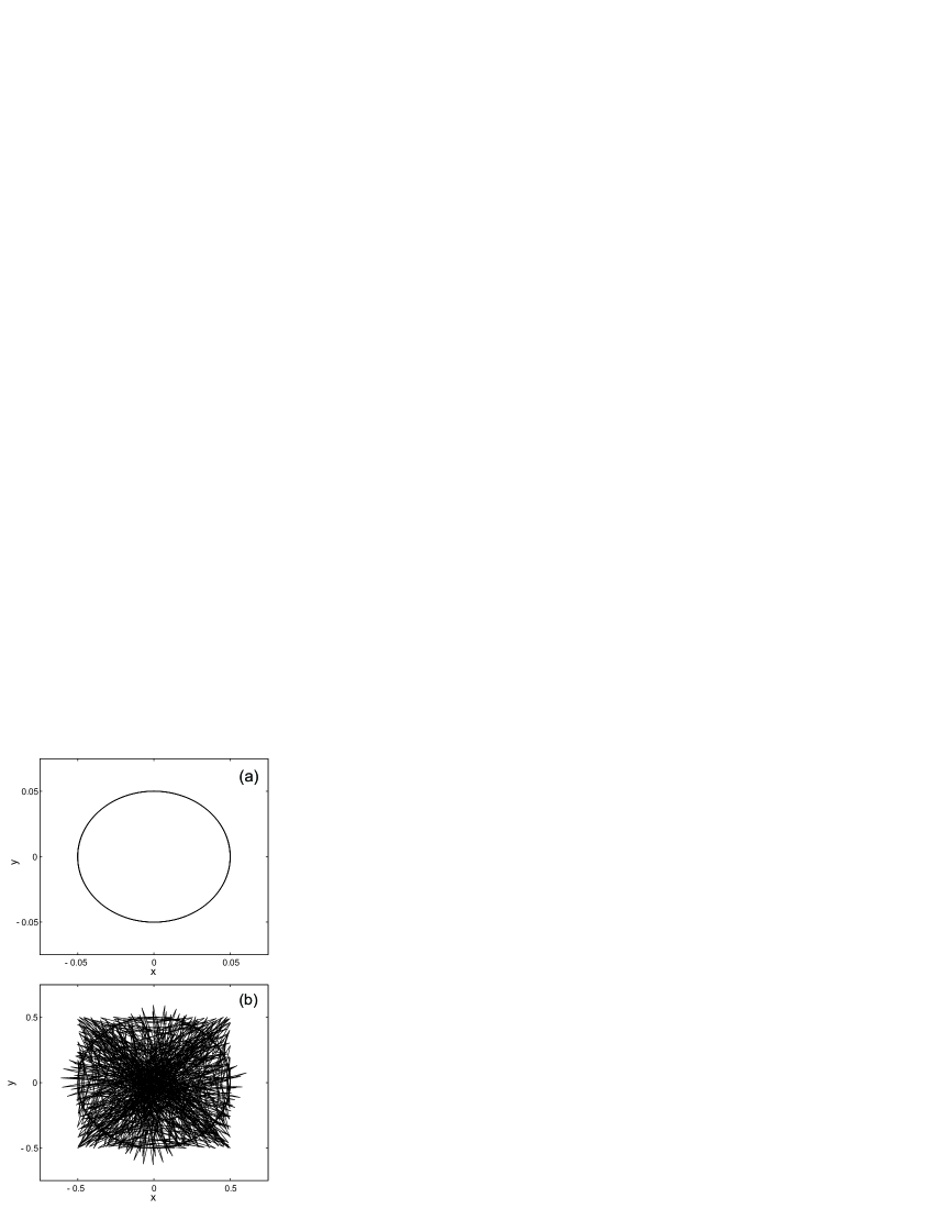
Figure 1: Particle trajectories integrated explicitly ($\alpha=0$) for the field $\bm{B}\left(\bm{x}\right)=\left[1+\left(x^{2}+y^{2}\right)/20\right]\bm{\hat{z}}$ put into the linear antisymmetric discretization gauge of the point $\left(0,0\right)$. A trajectory that remains close to $\left(0,0\right)$ is numerically stable (a), while further away (b), it is unstable because the local antisymmetric discretization gauge at $\left(0,0\right)$ is not a good approximation to the required gauge at the particle position.

II Electromagnetic gauge

In any physical system related to electromagnetism, dynamics must be invariant under an electromagnetic gauge transformation, $\bm{A}\left(\bm{x},t\right)\rightarrow\bm{A}\left(\bm{x},t\right)+\nabla\lambda\left(\bm{x},t\right)$, $\phi\left(\bm{x},t\right)\rightarrow\phi\left(\bm{x},t\right)-\partial_{t}\lambda\left(\bm{x},t\right)$. For the case of the single particle guiding center Lagrangian, Eq. (1), such a transformation is of course a special case of the gauge transformations considered in the previous section. Evidently continuous particle dynamics are invariant under a change of electromagnetic gauge. However, we have just illustrated that stability properties of the variationally discretized system can be strongly altered by gauge changes. Unlike traditional algorithms, in which the equations of motion (and thus $\bm{B}\left(\bm{x}\right)$ and $\bm{E}\left(\bm{x}\right)$) are discretized, the variational symplectic guiding center integrators are not electromagnetically gauge invariant. This can be illustrated explicitly (for the algorithm of Refs. Qin and Guan, 2008; Qin et al., 2009) by making the transformation $A_{i}^{\dagger}\rightarrow A_{i}^{\dagger}+\lambda_{,\,i}$, $\phi\rightarrow\phi-\partial_{t}\lambda$ in Eq. (3). This leads to the extra term,

$$\frac{1}{2h}\left[\lambda_{,\,ij}\left(x_{k+1}^{i}-x_{k-1}^{i}\right)-\left(\lambda_{,\,j}\left(\bm{x}_{k+1}\right)-\lambda_{,\,j}\left(\bm{x}_{k-1}\right)\right)\right]+\partial_{t}\lambda_{,\,j}\left(\bm{x}_{k}\right),$$ (21)

which is non-zero (but does of course vanish in the continuous limit). It is important to explore this further to understand limitations of the algorithm and how best to choose a gauge to obtain a reasonable approximation of particle motion.

The preceding considerations provide compelling motivation to: (i) restore gauge invariance to the discrete Lagrangian, (ii) compare this gauge invariant algorithm to the integrators from Refs. Qin et al., 2009; Qin and Guan, 2008; Li et al., 2011, and (iii), determine the conditions under which they should give a valid description of the motion. This can be achieved by replacing evaluations of $\bm{A}$ and $\phi$ at a single spacetime point (for instance $\left(\bm{x}_{k}+\bm{x}_{k+1}\right)/2$) with time integrals over a particle trajectory. For example, a discretized version of Eq. (1) that is gauge invariant is

$$L_{d} =\left[\int_{t_{k}}^{t_{k+1}}\frac{dt}{h}\bm{A}\left[\bm{x}\left(t\right)\right]+U_{k+\nicefrac{{1}}{{2}}}\bm{b}\left(\bm{x}_{k+\nicefrac{{1}}{{2}}}\right)\right].\left(\bm{x}_{k+1}-\bm{x}_{k}\right)/h$$

$$-\left[\int_{t_{k}}^{t_{k+1}}\frac{dt}{h}\phi\left[\bm{x}\left(t\right)\right]+\Gamma\left(\bm{x}_{k+\nicefrac{{1}}{{2}}},U_{k+\nicefrac{{1}}{{2}}}\right)\right].$$ (22)

Here, $\bm{x}_{k+\nicefrac{{1}}{{2}}}$ indicates $\left(\bm{x}_{k}+\bm{x}_{k+1}\right)/2$ and the path in the time integral, $\bm{x}\left(t\right)$, is simply a straight line between $\bm{x}_{k}$ and $\bm{x}_{k+1}$, that is, $\bm{x}\left(t\right)=\bm{x}_{k}+\left(\bm{x}_{k+1}-\bm{x}_{k}\right)\left(t-t_{k}\right)/h$. To prove gauge invariance of discrete equations of motion, we need to show that the discrete action, $\mathcal{S}_{d}=\sum_{k}L_{d}$, is unchanged (except at the endpoints) by an electromagnetic gauge transformation. For Eq. (22), first note that $\left(\bm{x}_{k+1}-\bm{x}_{k}\right)/h$ is $\bm{v}\left(t\right)$. The gauge transformation thus amounts to the addition of

$$\int_{t_{k}}^{t_{k+1}}\frac{dt}{h}\bm{v}.\nabla\lambda\left(\bm{x}\left(t\right),t\right)+\int_{t_{k}}^{t_{k+1}}\frac{dt}{h}\frac{\partial\lambda\left(\bm{x}\left(t\right),t\right)}{\partial t}$$ (23)

to Eq. (22). The first term is

$$\int_{t_{k}}^{t_{k+1}}\frac{dt}{h}\left[\frac{d\lambda}{dt}-\frac{\partial\lambda}{\partial t}\right],$$ (24)

the second part of which cancels the second term of Eq. (23). Carrying out the integral, we are left with

$$\lambda\left(\bm{x}_{k+1},t_{k+1}\right)-\lambda\left(\bm{x}_{k},t_{k}\right),$$ (25)

which contributes $\lambda\left(\bm{x}_{N},t_{N}\right)-\lambda\left(\bm{x}_{0},t_{0}\right)$ to $\mathcal{S}_{d}$. Since this is only a boundary contribution, the discrete equations of motion are unchanged and thus electromagnetically gauge invariant. Note that in a numerical implementation of the algorithm obtained from Eq. (22), the time integrals would need to be evaluated numerically. This calculation could be exact for piecewise polynomial $\bm{A}$ and $\phi$ (using Gaussian quadrature), as would be the case if they were defined discretely on some grid. Such discrete fields are used in many applications and an electromagnetically gauge invariant algorithm as introduced here could easily be implemented. As a side note, this is particularly important for use in a variational particle-in-cell scheme, where a particle pusher is coupled to an electromagnetic field solver in a single discrete variational principle. Ensuring electromagnetic gauge invariance of the discrete Lagrangian guarantees that the scheme satisfies the current continuity equation, $\partial_{t}\rho+\nabla\cdot\bm{J}=0$, which implies Gauss’s law remains satisfied at all timesSquire et al. .

II.1 Numerical example

The variational guiding center integrators considered use the discretizations $\bm{A}\left(\bm{x}\right)\rightarrow\frac{1}{2}\left[\bm{A}\left(\bm{x}_{k}\right)+\bm{A}\left(\bm{x}_{k+1}\right)\right]$ (Refs. Qin and Guan, 2008; Qin et al., 2009) or $\bm{A}\left(\bm{x}\right)\rightarrow\bm{A}\left(\bm{x}_{k+\nicefrac{{1}}{{2}}}\right)$ (Ref. Li et al., 2011). We would expect the lack of gauge invariance to be relatively unimportant if these terms (and similar terms for $\phi$) were good approximations to $\int_{t_{k}}^{t_{k+1}}\frac{dt}{h}\bm{A}\left[\bm{x}\left(t\right)\right]$, which is essentially an average of $\bm{A}$ over the particle trajectory. Thus, to minimise the consequences of the lack of electromagnetic gauge invariance on numerical results, we should choose a gauge such that the resulting $\bm{A}$ and $\phi$ are as smooth as possible. We note that this idea gives an answer to the question of how to implement the variational guiding center algorithms for a given magnetic field, perhaps defined on a grid. To ensure a stable algorithm, one should choose an $\bm{A}\left(\bm{x}\right)$ that is as smooth as possible under the constraint $\nabla\times\bm{A}=\bm{B}$.

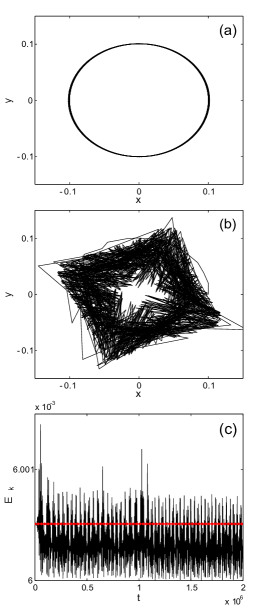
Figure 2: Numerically integrated particle trajectories in the field $\bm{B}\left(\bm{x}\right)=\left[1+\left(x^{2}+y^{2}\right)/20\right]\bm{\hat{z}}$: a) Using $\bm{A}=\left(-\frac{1}{60}y^{3},\,x+\frac{1}{60}x^{3},\,0\right)$, b) using $\bm{A}=\left(-\frac{1}{60}y^{3},\,x+\frac{1}{60}x^{3},\,0\right)+\nabla\cos\left(10\,xy\right)$. The kinetic energy, $E_{k}\left(t\right)$ is plotted in c), with the trajectory of a) in red, and that of b) in black. The time-step $h$ is chosen so that the particle rotates by approximately $1/10$ radians per timestep and the trajectory is integrated for 1000 timesteps.

We test out this idea numerically in Figure 2. This shows integrated guiding center particle trajectories for same magnetic field as the previous example, $\bm{B}\left(\bm{x}\right)=\left[1+\left(x^{2}+y^{2}\right)/20\right]\bm{\hat{z}}$. As before $\bm{A}=\left(-\frac{1}{60}y^{3},\,x+\frac{1}{60}x^{3},\,0\right)$ is used in Figure 2(a), while in Figure 2(b) we gauge transform this $\bm{A}$ with $\lambda=\cos\left(10\,x\,y\right)$. For the parameters of Figure 2(b), there will be a relatively large change in $\bm{A}\left(\bm{x}\right)$ over a timestep, meaning $\bm{A}\left(\bm{x}_{k+\nicefrac{{1}}{{2}}}\right)$ will not necessarily be an accurate approximation to $\int_{t_{k}}^{t_{k+1}}\frac{dt}{h}\bm{A}\left[\bm{x}\left(t\right)\right]$. This manifests itself in a highly unstable particle trajectory and kinetic energy [Figure 2(c)]. This property of the variational guiding center algorithms should not be problematic in practice provided a relatively smooth gauge is chosen and the time-step is sufficiently small. Numerical investigations have revealed that, as long as $\bm{A}\left(\bm{x}\right)$ and $\phi\left(\bm{x}\right)$ are not unusually uneven, timestep restictions are less severe than for conventional algorithms, such as fourth order Runga-Kutta.

III Conclusions and future work

The linear stability properties of the variational symplectic guiding center algorithms in Refs. Qin and Guan, 2008; Qin et al., 2009; Li et al., 2011 have been systematically examined to provide new insights into how these relate to gauge transformations of the governing Lagrangian. It was found that an oddity in the relationship between the discrete and continuous symplectic forms explains why explicit variational guiding center integrators have been observed to be numerically unstable. This can be mitigated by the use of an antisymmetric discretization gauge, in which even an explicit integrator is stable. However, this gauge does not always exist globally for realistic fields in general co-ordinates. Results from investigation of the consequences of the lack of electromagnetic gauge invariance in the variational symplectic guiding center algorithm indicate that as long as $\bm{A}\left(\bm{x}\right)$ is relatively smooth, the algorithm is approximately gauge invariant and should accurately reproduce particle dynamics.

There are still numerous properties and instabilities of the variational guiding center algorithm that require future work. One such instability, referred to in Ref. Li et al., 2011, affects the integrated parallel velocity, $u$, for fully 3-dimensional fields. The velocity is seen to oscillate between even and odd time-steps, with the amplitude growing in time. This instability is nonlinear, a complication for a systematic analysis, but can be mitigated by formulating the algorithm in terms of $u_{k+1/2}\equiv\left(u_{k}+u_{k+1}\right)/2$ rather than $u_{k}$. Another area of ongoing research is in variational integrators for fields defined discretely on a grid, as would be required, for example, if the magnetic field is output from another code. Preliminary results show certain numerical instabilities associated with the piecewise nature of $\bm{A}$. The results presented above on electromagnetic gauge transformations may be important in such studies, and investigations into gauge invariant integrators are ongoing.

References

- Qin and Guan (2008) H. Qin and X. Guan, Phys. Rev. Lett. 100, 035006 (2008).
- Qin et al. (2009) H. Qin, X. Guan, and W. Tang, Phys. Plasmas (2009).
- Li et al. (2011) J. Li, H. Qin, Z. Pu, L. Xie, and S. Fu, Phys. Plasmas 18, 052902 (2011).
- (4) J. Squire, H. Qin, and W. Tang, (to be published).
- Littlejohn (1983) R. G. Littlejohn, J. Plasma Physics 29, 111 (1983).
- Lin et al. (1998) Z. Lin, T. S. Hahm, W. W. Lee, W. M. Tang, and R. B. White, Science 281, 1835 (1998).
- Chen and Parker (2003) Y. Chen and S. E. Parker, Journal of Computational Physics 189, 463 (2003).
- Cohen et al. (1980) B. I. Cohen, T. A. Brengle, D. B. Conley, and R. P. Freis, Journal of Computational Physics 38, 45 (1980).
- Veselov (1988) A. P. Veselov, Functional Analysis and Its Applications 22, 83 (1988).
- Channell and Scovel (1990) P. J. Channell and C. Scovel, Nonlinearity 3, 231 (1990).
- Candy and Rozmus (1991) J. Candy and W. Rozmus, Journal of Computational Physics 92, 230 (1991).
- Feng (1986) K. Feng, J. Comput. Math. 4, 279 (1986).
- Yoshida (1990) H. Yoshida, Physics Letters A 150, 262 (1990).
- Marsden and West (2001) J. E. Marsden and M. West, Acta Numerica 10, 357 (2001).
- Reich (1999) S. Reich, SIAM J. Numer. Anal. 36, 1549 (1999).
- Cary and Littlejohn (1983) J. R. Cary and R. G. Littlejohn, Annals of Physics 151, 1 (1983).
- Rowley and Marsden (2002) C. Rowley and J. Marsden, in Decision and Control, 2002, Proceedings of the 41st IEEE Conference on, Vol. 2 (2002) pp. 1521 – 1527 vol.2.
- Grebogi and Littlejohn (1984) C. Grebogi and R. G. Littlejohn, Physics of Fluids 27, 1996 (1984).
- White and Zakharov (2003) R. White and L. E. Zakharov, Physics of Plasmas 10, 573 (2003).