On a Voter model on :
Cluster growth in the
Spatial -Fleming-Viot Process
Abstract
The spatial -Fleming-Viot (SFV) process introduced in (Barton, Etheridge and Véber, 2010) can be seen as a direct extension of the Voter Model (Clifford and Sudbury, 1973); (Liggett, 1997). As such, it is an Interacting Particle System with configuration space , where is the set of probability measures on some space . Such processes are usually studied thanks to a dual process that describes the genealogy of a sample of particles. In this paper, we propose two main contributions in the analysis of the SFV process. The first is the study of the growth of a cluster, and the suprising result is that with probability one, every bounded cluster stops growing in finite time. In particular, we discuss why the usual intuition is flawed. The second contribution is an original method for the proof, as the traditional (backward in time) duality methods fail. We develop a forward in time method that exploits a martingale property of the process. To make it feasible, we construct adequate objects that allow to handle the complex geometry of the problem. We are able to prove the result in any dimension .
keywords:
[class=AMS]keywords:
t1Supported by EPSRC Grant EP/E065945/1. t2The author would like to thank Alison Etheridge, Nic Freeman and Mladen Savov for carefully reading earlier versions of this manuscript.
1 Introduction
The spatial -Fleming-Viot process (SFV) is a model
used
to represent biological evolution on a continuum.
It was first
introduced in [7],
and then studied in more details in [1] ,
[2] and [3].
In this setting, given a set of genetic types , a population
living on is represented by a collection of probability measures on .
More precisely, the genetic composition at time of the population at point
is given by a measure on the type space .
The SFV process
is a direct spatial extension of the generalised Fleming-Viot processes presented in [6] and
studied in [4].
But it can also be seen as an
interacting particle system generalising
the Voter Model [5, 8].
The configuration space for the Voter Model is , whereas for the SFV process
it is , where is the
set of probability measures on . This generalisation of the configuration space is one of the elements
that make the study of the SFV process particularly challenging.
Our motivation in this article is the study of the fate of a new genetic type created by mutation at time . More precisely, we assume that there are only two types of individuals, and , and that the new type, say , occupies a bounded set of at time . The question is how far this newly created type is going to spread.
Because we are working with two types only, the setting simplifies. We have , so at time it is enough to consider the collection of numbers . This is why we are going to represent the population at time by the function
such that . Working with a function instead of a collection of probability measures allows us to simplify the notation when manipulating the SFV process.
1.1 The process
For every time , let be a function from to . The quantity for is the frequency of individuals at location . The dynamics of is the following. Consider a space-time Poisson point process on with rate , and two constants and . Then, for every point of ,
-
i)
Draw a ball of radius centred around .
-
ii)
If , then the parent is , and for every point ,
-
iii)
If , then the parent is , and for every point ,
The steps i), ii) and iii) can be written in a single equation:
| (1) |
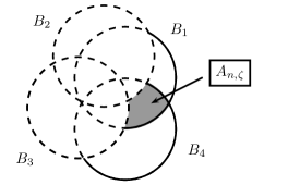
In biological terms, each point of the Poisson Point process corresponds to a reproduction event taking place at time in a ball . First, a parent is chosen at random at location . The parent is with probability and with probability , and her offspring are going to have the same type as her. Second, competition for finite resources causes a proportion of the population inside the ball of centre and radius to die. Finally, the offspring of the parent replaces the proportion of individuals who have died. Births and deaths take place simultaneously at time . Figure 1 illustrates the births and deaths events taking place during a single transition at time corresponding to the point from the Poisson point process .


Remark 1.1.
We have chosen the parent to be at location , which is a simplification of the model in [2], where the location of the parent was chosen uniformly on the ball. This does not change the model significantly, it just simplifies some calculations.
The presentation of the process we just gave is simply an algorithm that describes the jumps of , but we need to construct it formally as a Markov process. The most natural way is to translate this algorithm into the infinitesimal generator of , which is defined by
| (2) |
where is a test function, and is the initial value of the process . We choose the test function from the family of functions of the form
| (3) |
where is a function from to such that , and is a function from to corresponding to . The intuition behind this form is that the distribution of the function-valued process is described by the finite-dimensional dynamics at all locations .
The generator of the process is given by
| (4) |
To understand this expression, we can think of as a jump process with possibly an infinite number of jumps at each instant. The transitions of the process are indexed by the points of the Poisson Point process with intensity . Morally, we can use equation (1) and write the generator in the form
where
When we replace the test functions with their expression, we obtain
To express the integral
we find the unique set that verifies if and only if (see figure 2 ). After careful computations, we obtain expression (4).

One needs to prove that there exists a Markov process that is defined by (4). A general proof for the existence of the SFV process is given in [2] using duality. However, we do not need to use this result, because in our case we are able to construct directly the process using our forward in time method, see §5.3.
1.2 Main result
The bounded support population is competing against the unbounded support population, so intuitively, we expect the population to become extinct. The real question is how far the population manages to spread before ultimately disappearing. This is why we are studying the dynamics of the support of the population.
Every time the individual sampled to be the parent is not , the proportion of the population decreases, which decreases the overall probability that the parent at the next event is going to be . The same reasoning applies to the population. The only way for the support to grow is if the ball of centre and radius is not entirely contained in the support of , while the parent sampled at is . On the other hand, if we take , the support never shrinks, as once a point is occupied with a frequency , its future frequencies will always be positive.
Given this schematic view of the dynamics of the process, one intuitively expects a behaviour similar
to what we are going to call the oil film spreading:
The proportion of the population would converge to zero at every point, but at the same time
its support would grow
forever and ultimately would occupy an infinite subset of . Stated more naturally, there seems to be no reason
why the support would not grow to an infinitely large set.
However, the actual behaviour of the process is rather counterintuitive. Before stating our main result,
we need to introduce some notation.
Notation 1.2.
-
•
For any given function , we denote its support by Supp.
-
•
We define to be the set of Borel measurable functions with compact support. We endow with the norm.
-
•
Given a set and , we denote by the -expansion of , that is the set defined by
Theorem 1.3.
Let be a Markov process with generator (4). Suppose is deterministic and with bounded support. Then, there exists a random finite set , and an almost surely finite random time such that
| (5) |
Furthermore,
| (6) |
Remark 1.4.
For the sake of clarity, we chose to be deterministic. The result would still be true if , see Remark 4.12.
The proof of this result is the objective of this paper. It is fairly challenging because of the large dimension of the
state space. Although the result is stated for the support of , the actual object we need to keep track of
is the whole function . The natural approach consisting in approximating probabilities of trajectories that correspond to the event
in question simply do not work, because such approximations waste too much information about the process.
Our approach is to first summarise the structure
of the process in a useful way. This is why we build adequate geometric tools that allow us to use a powerful martingale argument.
Fundamentally, the cause of the behaviour described in Theorem 1.3 lies in the discrete nature of the jumps inherent to FV processes, rather than in the geometry of the SFV process.
To see that, we consider the simpler process where there is no space, that is to say at every reproduction event, the parent is sampled with probability , and a proportion of the whole population is replaced by the offspring of the parent. In the notation of [4], the process is the FV process on the state-space with -measure . It is a continuous time Markov Chain on with constant intensity, and the transitions of its embedded discrete time Markov Chain are given by
where is a Bernoulli distribution with parameter . It is straightforward to show that is a nonnegative martingale, and therefore converges almost surely. As a consequence, converges almost surely to or . This means that after some finite random time, will remain constant equal to or . Almost surely in finite time, either the or the population will be the only one to keep reproducing.
This remarkable feature is due to the fact that if the frequency is
not sampled
a few
times in a row, it is going to decrease geometrically, and becomes rapidly too small
to be
sampled again. The same reasoning applies to the population.
As we will prove, the same mechanism takes place in the spatial model, that is after some almost surely finite random time, the population will stop reproducing.
1.3 Proofs and outline
The martingale argument we demonstrated in the previous section seems to be the most promising approach. However, to be able to use such an argument, we need to find a way to filter out all the complex dependencies introduced by space, which is the main challenge in this work. We solved this problem by introducing in §4.2 the geometrical object of forbidden region that allows to connect the martingale convergence to the sampling of the population.
The rest of this article is devoted to the proof of Theorem 1.3, as well as the construction of the process defined by (4).
In Section 2, we introduce a discrete time Markov Chain which is the discrete time equivalent of . This chain is going to be used to construct and to prove Theorem 1.3. We state in Proposition 2.5 the equivalent of Theorem 1.3 in discrete time.
Section 3 provides a toolbox that allows to handle easily the geometry of the model.
We prove in Section 4.3 the central Proposition 4.11, which states that in discrete time, the population defined by is sampled from only finitely many times. The proof relies on the fact that the total mass of the population, i.e. the integral of over , is a martingale that converges almost surely. In §4.2, we introduce the crucial concept of forbidden region, and use it to prove Proposition 4.11.
We gather all the results in Section 5 . Proposition 4.11 allows both to use to construct as a non explosive continuous time Markov Chain, and to prove Theorem 1.3.
We finally conclude by discussing some extensions of this work.
2 A discrete time Markov chain
2.1 Construction
Definition 2.1.
Consider and . Let be an -valued random variable. We construct simultaneously random sequences and , a filtration , and an -valued Markov chain , using the following recurrence:
| (7) |
and for ,
-
•
,
-
•
conditionally on , is uniform on ,
-
•
is distributed uniformly on , independently from and ,
-
•
is given by the formula
(8) -
•
.
We introduce the notation . In particular, the trajectories of are given by
| (9) |
Finally, we denote the natural filtration of by .
Remark 2.2.
We recall that is the -expansion of the set .
At each reproduction event, the random variable corresponds to the centre of the event. The parent is sampled uniformly at location thanks to the random variable , so that the parent is with probability , and with probability . The constants and are the radius of the event and the proportion of the population that is modified. The random variable indicates the types of the parent chosen.
Notation 2.3.
If , we say that the event is a positive sampling event, because the total red population increases, whereas when we say that it is a negative sampling event.
Equation (9) shows that if the cluster
is to increase, the
minimum requirement is that there is a positive sampling.
Remark 2.4.
Expression (9) is true because we assumed . In this case, the support and the range of the process coincide. Once a region is occupied by the Red population it remains occupied at every finite time. Therefore the cluster never shrinks. In the case where expression (9) would remain true if was defined to be the range of the process, that is .
2.2 Result of the cluster convergence
The following result is the expression of our main result in the discrete time setting, with the temporary technical condition . This condition is removed in Proposition 5.1 by allowing to be any deterministic function with bounded support.
Proposition 2.5.
Suppose , where , and . Then, there exists an almost surely finite random time such that
| (10) |
Therefore, there exists an almost surely bounded random set such that
| (11) |
Most of the remainder of this paper is devoted to proving this Proposition. We first investigate the geometric properties of the model in the next section.
3 Geometry
This section constructs all the tools that allow us to manage the geometry of the process.
Remark 3.1.
From now on, unless specified otherwise, we suppose that .
3.1 is piecewise constant
Definition 3.2.
For notational convenience, we introduce the sequence
such that
| (12) |
Lemma 3.3.
For every , for every , consider the set defined by
| (13) |
The function can be written as
| (14) |
where the sets are all disjoint for a given , and .
Remark 3.4.
By construction, , we have .
Proof.
We first introduce the shorter notation
The fact that the sets are all disjoint for a given is straightforward, so we just need to prove (14). But before that, we need to show that
| (15) |
and we proceed by induction on . The statement is true for . Suppose now that it is true for some given . Let .
-
–
If , then
-
–
If , and then there exists such that
-
–
If , then there exists such that
Therefore, we see that
and the statement is proven using the inductive hypothesis.
We can return to the proof of expression (14). We need to show that for all , ,
| (16) | ||||
| and | ||||
| (17) |
We prove (16) by induction on , and we use (15). Statement (16) is satisfied for because . Suppose now that it is true for some , and consider . In particular, , and using the dynamics equation (8), we find that Because , we can use the inductive hypothesis, and we obtain that , which proves (16).
To prove (17), we also use induction. It is true for . Suppose (17) is satisfied for a given . Consider , and take .
- –
-
–
If and , there exists such that
Therefore , and using the inductive hypothesis, we have .
-
–
If , then there exists such that
In this case , and using the inductive hypothesis, we have .
We can express using the dynamics equation (8), and we obtain:
We have proved that for any choice of , all the terms in the above equations are the same for and , therefore , and we have proved (17). ∎
3.2 Variation of the local average
A central tool for the rest of the work is the average of the function on a ball of radius and centre . It is important that is the radius of the reproduction event, as this is what links the martingale introduced in the next section to the geometry of the process (see Lemma 4.2). We introduce the following function:
Definition 3.5.
| (18) |
The main result of this section is the following.
Proposition 3.6.
For every ,
| (19) |
The rest of this section is devoted to proving this inequality. For this we need to introduce some auxiliary functions.
Definition 3.7.
Given , for every , we define
| (20) | ||||
The key property for the proof of Proposition 3.6 is the following.
Proposition 3.8.
is a continuous, piecewise differentiable function. Moreover, for every point where is differentiable, we have:
| (21) |
Proof.
We first prove that is continuous and that there is at most a finite number of points at which is not differentiable. Thanks to equation (14) from Lemma 3.3, we see that is given by
therefore is given by
| (22) |
We simplify the notation by introducing and
The definition (13) of the sets and the inclusion-exclusion formula allow us to prove that for each , there exists a such that
Remark 3.9.
The main change with expression (22) is that now we are working with intersections of balls, which are convex, whereas the sets are usually not. Also, we had the fact that is the value of the function on the set , and such an interpretation is lost for .
If we introduce the function defined for each set by
| (23) | ||||
then we can simply rewrite the function as
| (24) |

The continuity of follows from the continuity of
the function , and this shows that
is continuous.
The set is convex, therefore there exist , such that
| (25) |
Consider such that . Thanks to (25), this means we can choose a point belonging to the interior of . Because the set is convex, we can express its volume in -dimensional spherical coordinates with as the new origin. Given angular coordinates , we denote by the unique point of the boundary of with angular coordinates , and the distance between and . We have:

We denote by the boundary of , and by the sphere of centre and radius . We can find a partition of the space
such that
Therefore we can write as
Thanks to this representation, we see that a sufficient condition for to be differentiable at , , is that for every in the interior of every , the function is differentiable at . In this case, the derivative is given by
We focus now on the differentiability of , where belongs to the interior of for some .
Suppose first that . Because the function is continuous, and because is a fixed point, there exists such that for every , . Therefore, there exists such that for every , , and is differentiable at .
In the case where , by the
same continuity argument, we obtain that for every ,
. Because the distance between and the
projection of on along the angle is differentiable,
we conclude that is also differentiable in
this case.
We have proved that for all , is differentiable at . Given that
we conclude that there is at most a finite number of points at which
is not differentiable, and this proves the first
part of the
Proposition.
We need now to show the upper bound (21) for the derivative. Suppose is differentiable at . By definition,
therefore
By construction, for all , , which implies that
Dividing by and taking the limit as , we obtain
| (26) |
where is the volume of a ball of radius , and its surface area. ∎
4 Probability
4.1 A martingale argument
Definition 4.1.
We denote by the total mass of , that is
Lemma 4.2.
The change of the total mass is given by
| (27) |
Proof.
Using (8),
Proposition 4.3.
is a discrete time nonnegative martingale.
Proof.
In particular, for every ,
so , which shows that is a martingale. ∎
Definition 4.4.
Let be a real number such that . We then define
| (28) |
In particular, is not a stopping time, but this is not going to be an issue in what follows.
Proposition 4.5.
The random time is a.s. finite, and ,
| (29) |
Proof.
We know that is a nonnegative martingale, so it converges almost surely when . Therefore is almost surely finite, and by definition, . Using Lemma 4.2, we observe that
which concludes the proof. ∎
4.2 Forbidden region
The concept of a forbidden region will allow us to treat probabilistically the geometric properties established in §3.
Lemma 4.6.
For ,
| (30) |
Proof.
Take such that . Using Proposition 4.5, this implies that . In particular, . By induction, we just showed that
The contrapositive of this implication allows to conclude this proof. ∎
Definition 4.7.
We define the forbidden region to be
| (31) |
We also introduce the quantity
| (32) |
The reason for the name forbidden region is motivated by the following lemma, which tells us that after the time , if the local averages are always too high, then the points are forbidden from falling in the region . Furthermore, this lemma provides a lower bound on the volume of .
Lemma 4.8.
| (33) |
Proof.
An immediate consequence of Proposition 4.5 is
More work is required to obtain the lower bound for the volume of the forbidden region. We first define . If we assume , then is nonempty. We can then take a point .
The function is continuous, and is finite, so the region is infinite. Indeed, for every at a distance from larger than , . In particular, for a large enough positive number , we can consider the sphere of radius and centre , and the ball such that
| (34) |
For , we denote by the line-segment between and . We need the following lemma:
Lemma 4.9.
The point being fixed, for every point , we can find two points such that:
| (35) |
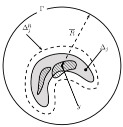
By integrating the result of Lemma 4.9 over all the points , we find that the volume of is larger than the volume of a ball of radius , hence the result. ∎
Proof of Lemma 4.9.
We reach now the main point of this section, which is an upper bound for the probability that infinitely many positive sampling events take place.
Proposition 4.10.
| (36) |
4.3 Finitely many positive sampling events
Proposition 4.11.
Proof.
Using Proposition 4.10, we simply need to prove that for every ,
By monotone convergence, we have
We are going to work in the slightly more general setting where , and therefore , are allowed to be random. This is easily dealt with, because we begin by conditioning on :
We then condition on all but the last reproduction events:
| (39) | ||||
We can calculate the last term by conditioning on and :
| (40) |
The second and third equalities come from the fact that conditionally on , is sampled uniformly from , independently of the past. The last inequality comes from (9):
In particular, it implies that
Putting inequality (40) into (39), we obtain the following upper bound:
| (41) |
Inequality (41) provides a recurrence relation, which we can solve immediately to obtain
Taking expectation and then the limit as , we obtain
We rewrite the infinite random product using logarithms:
After observing that
we conclude that the infinite product is almost surely equal to . Because we chose to be deterministic, we conclude that
∎
Remark 4.12.
In the case where we take to be random, a sufficient condition for the expectation of the infinite product to also be equal to is simply , that is the volume of the initial support has a finite expectation.
5 Proof of the theorems
5.1 Proof of Proposition 2.5
We proved in Proposition 4.11 that with probability one, there are only finitely many sampling events. This means that there exists an almost surely finite random time such that
| (42) |
We recall the dynamics of the cluster described by (9):
Therefore, if we define , we have
| (43) |
and the proof of Proposition 2.5 is complete.
We can now generalise Proposition 2.5 by removing the technical condition on the starting point and allowing to be any function in .
Proposition 5.1.
Suppose . Then, there exists an almost surely finite random time such that
| (44) |
Therefore, there exists an almost surely bounded random set such that
| (45) |
Proof.
We proceed by coupling with a Markov chain with the same transition probabilities, but started from such that . We denote the initial conditions by and . We first build as described in Definition 2.1. We then use the sequences and that we used to construct in the following way. First consider the random sequence defined by , and for ,
We can prove by induction that
| (46) |
It is of course true at , and then we just observe that if , then
We denote by and the respective sequences of supports, and in particular we have proved that
| (47) |
We define the sequence of -stopping times by setting
| (48) |
We now construct , and by taking
We denote by the support of , and we define the filtration to be
By construction, conditionally on , is distributed uniformly on . Because is independent of , we conclude that the law of is the one given in Definition 2.1.
Using (46), we see that
| (49) |
We introduce
Because , we can use Proposition 2.5, and we obtain that there exists almost surely finite such that
| (50) |
In particular, this implies that there exists almost surely finite such that
| (51) |
Combined with (49), this implies that
| (52) |
and the conclusion follows. ∎
5.2 The continuous time process is non explosive
We are now going to construct explicitly the process with generator (4) as a continous time Markov chain, by using as the embedded Markov chain.
Definition 5.2.
Consider an i.i.d sequence of Exp(1) random variables. We define the jump times by setting and
| (53) |
where for .
We can then define a stochastic process
by setting
| (54) |
We recall that the set is the -expansion of the support of , that is the set of points at a distance less than from the support of . The quantity is its volume, and it is the rate at which the process jumps out of the state . This will be verified in the following proposition by checking that we have the correct generator.
Proposition 5.3.
Proof.
The first thing to verify is that is really defined for all nonnegative . This is equivalent to saying that
that is
We show in Proposition 2.5 that converges in a finite number of steps to a bounded set . This means that almost surely, there is a random time such that for all ,
which implies that
Hence is a stochastic process defined for all . The Markov property is obvious, and this shows that is a non-explosive continuous time Markov chain. We can then write the generator of for functions as
If we take as defined in (3), the generator of takes the form (4). ∎
5.3 Proof of Theorem 1.3
We have seen in Proposition 5.3 that the process is a non explosive continuous time Markov chain. Therefore, the trajectories of are completely described by its embedded Markov chain .
In particular, for all , for all , . Using the result from Proposition 5.1, and the the sequence of times defined in (53), there exists a finite random set , and an almost surely finite random time , such that
| (55) |
The second point to prove here is the extinction of the population. From Proposition (5.1),
| (56) |
This implies that at every point , the frequency converges geometrically to zero, which concludes the proof.
6 Conclusion
Although the SFV process is constructed in great generality, our study was restricted to the case where and are constant. In the setting described in [2], these quantities can be made random by adding extra dimensions to the space-time Poisson point process. We then define on the space , with intensity , such that
Our result holds in the case because the volume of increases at most linearly with . We could imagine extending the same result using practically the same method to the case where
because the process still jumps at finite rate, and the
volume of is at most of order , where
is a realisation of the random radius. The problem comes from
the fact that the radii being random makes the construction
of the Markov chain more complicated. Morally the result remains true
in this case, but the proof becomes significantly more involved.
The situation where
is radically different, because now the process jumps at an infinite rate. The problem is that we do not have a description of the geometry of the process at time . The behaviour is not obvious, and it cannot be simulated. For us this remains an open question, which would certainly require different techniques.
References
- [1] N. H. Barton, A. M. Etheridge, and J. Kelleher. A new model for extinction and recolonization in two dimensions: quantifying phylogeography. Evolution, 64:2701–2715, 2010.
- [2] N. H. Barton, A. M. Etheridge, and A. Véber. A new model for evolution in a spatial continuum. Electronic Journal of Probability, 15:162–216, 2010.
- [3] N.. Berestycki, A. M. Etheridge, and A. Véber. Large scale behaviour of the spatial Lambda-Fleming-Viot process. http://arxiv.org/abs/1107.4254, 2011.
- [4] J. Bertoin and J. F. Le Gall. Stochastic flows associated to coalescent processes. Probability Theory and Related Fields, 126:261–288, 2003.
- [5] P. Clifford and A. Sudbury. A model for spatial conflict. Biometrika, 60:581–588, 1973.
- [6] P. Donnelly and T.G. Kurtz. Particle representations for measure-valued population models. Annals of Probability, 27:166–205, 1999.
- [7] A. M. Etheridge. Drift, draft and structure: some mathematical models of evolution. Banach Center Publications, 80:121–144, 2008.
- [8] T.M. Liggett. Stochastic models of interacting systems. Annals of Probability, 25:1–29, 1997.