Neutron Star Powered Nebulae: A New View on Pulsar Wind Nebulae with the Fermi Gamma-ray Space Telescope

NEUTRON STAR POWERED NEBULAE: A NEW VIEW ON PULSAR WIND NEBULAE WITH THE FERMI GAMMA-RAY SPACE TELESCOPE

A DISSERTATION
SUBMITTED TO THE DEPARTMENT OF PHYSICS
AND THE COMMITTEE ON GRADUATE STUDIES
OF STANFORD UNIVERSITY
IN PARTIAL FULFILLMENT OF THE REQUIREMENTS
FOR THE DEGREE OF
DOCTOR OF PHILOSOPHY

© Copyright by Joshua Jeremy Lande 2024
All Rights Reserved

I certify that I have read this dissertation and that, in my opinion, it is fully adequate in scope and quality as a dissertation for the degree of Doctor of Philosophy.

  (Stefan Funk) Principal Adviser

I certify that I have read this dissertation and that, in my opinion, it is fully adequate in scope and quality as a dissertation for the degree of Doctor of Philosophy.

  (Elliott Bloom)

I certify that I have read this dissertation and that, in my opinion, it is fully adequate in scope and quality as a dissertation for the degree of Doctor of Philosophy.

  (Roger Romani)

Approved for the University Committee on Graduate Studies

 

“Two things fill the mind with ever-increasing wonder and awe, the more often and the more intensely the mind of thought is drawn to them: the starry heavens above me and the moral law within me.”

– Immanuel Kant

Abstract

Pulsars are rapidly-rotating neutron stars born out of the death of stars. A diffuse nebula is formed when particles stream from these neutron stars and interact with the ambient medium. These pulsar wind nebulae (PWNe) are visible across the electromagnetic spectrum, producing some of the most brilliant objects ever observed. The launch of the Fermi Gamma-ray Space Telescope in 2008 has offered us an unprecedented view of the cosmic $\gamma$-ray sky. Using data from the Large Area Telescope on board Fermi, we search for new $\gamma$-ray-emitting PWN. With these new observations, we vastly expand the number of PWN observed at these energies. We interpret the observed $\gamma$-ray emission from these PWN in terms of a model where accelerated electrons produce $\gamma$-rays through inverse Compton upscattering when they interact with interstellar photon fields. We conclude by studying how the observed PWN evolve with the age and spin-down power of the host pulsar.

Chapter 1 Overview

In Chapter 2, we discuss the history of $\gamma$-ray astrophysics. First we present broadly the history of astronomy in Section 2.1 and the history of $\gamma$-ray astrophysics in Section 2.2. Then, we discuss the Fermi Gamma-ray Space Telescope in Section 2.3. Next, we discuss historical developments in our understanding of pulsars and pulsar wind nebula (PWN) in Section 2.4. We conclude by discussing the major source classes detected by the Large Area Telescope (LAT) in Section 2.5 adn the major radiation processes that occur in high-energy astrophysics in Section 2.6.

In Chapter 3, we discuss our current understanding of the physics of pulsars and PWN. We discuss the formation of a pulsar in Section 3.1 and the time evolution of a pulsar in Section 3.2. Then, we describe the magnetosphere of the pulsar in Section 3.3 and the structure of a typical PWN in Section 3.4. Finally, we describe the energy spectrum emitted from a typical PWN in Section 3.5.

In Chapter 4, we discuss maximum-likelihood analysis and how it can be used to analyze LAT data. We describe the motivation for using maximum-likelihood analysis in Section 4.1 and the maximum-likelihood formulation in Section 4.2. Then, we describe how to build a model of the $\gamma$-ray sky in Section 4.3 and describe the LAT instrument response functions (IRFs) in Section 4.4. Finally, we describe the standard package $\mathtt{gtlike}$ for performing maximum-likelihood analysis of LAT data in Section 4.5 and we describe $\mathtt{pointlike}$, an alternate package for performing maximum-likelihood analysis of LAT data, in Section 4.6.

In Chapter 5, we discuss a new method to study spatially-extended sources. We discuss the formulation of this method in Section 5.2. We validate the extension-significance calculation in Section 5.3 and then we compute the sensitivity of the LAT to spatially-extended sources in Section 5.4. We develop a new method to compare the hypothesis of multiple point-like sources to one spatially-extended source in Section 5.5 and finally in Section 5.6 we validate our method by testing point-like sources from the second LAT AGN catalog (2LAC) for extension.

In Chapter 6, we apply the extension test developed in Chapter 5 to search for new spatially-extended sources. First, we validate the method by studying known spatially-extended LAT sources in Section 6.1.

In Section 6.2, we develop a method to estimate systematic errors associated with studying extended sources and in Section 6.3 we develop a method to search for new spatially-extended sources. Finally, we discuss the newly-discovered spatially-extended sources in Section 6.4 and the population of spatially-extended LAT sources in Section 6.5.

In Chapter 7, we perform a search for new PWN in the off-peak regions of LAT-detected pulsars. First, we develop a new method to define the off-peak regions used for the search in Section 7.1. Then, we describe the analysis method we used to search these regions in Section 7.2 and the results of this search in Section 7.3. Finally, we discuss some of the sources detected with this method in Section 7.4.

In Chapter 8, we perform a search for $\gamma$-ray emission from very high energy (VHE) PWN. We discuss our list of VHE candidates in Section 8.1 and our analysis method in Section 8.2. Finally, we several new PWN detected using this method in Section 8.3.

In Chapter 9, we describe the population of $\gamma$-ray emitting PWN and study how they evolve with the spin-down energy and age of their associated pulsars. Finally, in Chapter 10 we remark on potential future opportunities to expand our understanding of PWNe and their $\gamma$-ray emission.

Chapter 2 Gamma-ray Astrophysics

2.1 Astronomy and the Atmosphere

From the very beginning, humans have surely stared into space and contemplated its brilliance. Stone circles in the Nabta Playa in Egypt are likely the first observed astronomical observatory and are believed to have acted as a prehistoric calendar. Dating back to the 5th century BC, they are 1,000 years older than Stonehenge (McK Mahille et al. 2007).

Historically, the field of astronomy concerned the study of visible light because it is not significantly absorbed in the atmosphere. But slowly, over time, astronomers expanded their view across the electromagnetic spectrum. Infrared radiation from the sun was first observed by William Herschel in 1800 (Herschel 1800). The first extraterrestrial source of radio waves was detected by Jansky in 1933 (Jansky 1933). The expansion of astronomy to other wavelengths required the development of rockets and satellites in the 20th century. The first ultraviolet observation of the sun was performed in 1946 from a captured V-2 rocket (Baum et al. 1946). Observations of x-rays from the sun were first performed in 1949 (Burnight 1949).

2.2 The History of Gamma-ray Astrophysics

It was only natural to wonder about photons with even higher energies. As is common in the field of physics, the prediction of the detection of cosmic $\gamma$-rays proceeded their discovery. Feenberg & Primakoff (1948) theorized that the interaction of starlight with cosmic rays could produce $\gamma$-rays through inverse Compoton (IC) upscattering. Following the discovery of the neutral pion in 1949, Hayakawa (1952) predicted that $\gamma$-ray emission could be observed from the decay of neutral pions when cosmic rays interacted with interstellar matter. And in the same year, Hutchinson (1952) discussed the bremsstrahlung radiation of cosmic-ray electrons. Morrison (1958) predicted the detectability of $\gamma$-ray emission from solar flares, PWNe, and active galaxies.

The first space-based $\gamma$-ray detector was Explorer XI (Kraushaar et al. 1965). Explorer XI operated in the energy energy range above $100\,\text{MeV}$. It had an area of $\sim 45\text{cm}^{2}$ but an effective area of only $\sim 7\text{cm}^{2}$, corresponding to a detector efficiency of $\sim 15\%$. It was launched on April 27, 1961 and was in operation for 7 months. Explorer XI observed 31 $\gamma$-rays but, because the distribution a distribution of these $\gamma$-rays was consistent isotropy, the experiment could not firmly identify the $\gamma$-rays as being cosmic.

The first definitive detection of $\gamma$-ray came in 1962 by an experiment on the Ranger 3 moon probe (Arnold et al. 1962). It detected an isotropic flux of $\gamma$-rays in the 0.5 MeV to 2.1 MeV energy range.

The Third Orbiting Solar Observatory (OSO-3) was the first experiment to firmly identify $\gamma$-ray emission from the Galaxy (Kraushaar et al. 1972). OSO-3 was launched on March 8, 1967 and operated for 16 months, measuring 621 cosmic $\gamma$-rays. Figure 2.1 shows a sky map of these $\gamma$-rays. This experiment confirmed both a Galactic component to the $\gamma$-ray sky as well as an additional isotropic component, hypothesised to be extragalactic in origin.

Figure 2.1: The position of all 621 cosmic $\gamma$-rays detected by OSO-3. This figure is from Kraushaar et al. (1972).

This anisotropic $gamma$-ray distribution was confirmed by a balloon-based $\gamma$-ray detector in 1970 (Kniffen & Fichtel 1970). In the following year, the first $\gamma$-ray pulsar (the Crab pulsar) was detected by another balloon-based detector Browning et al. (1971).

The next major advancements in $\gamma$-ray astronomy came from the second Small Astronomy Satellite (SAS-2) and COS-B. SAS-2 was a dedicated $\gamma$-ray detector launched by the National Aeronautics and Space Administration (NASA) in November 15, 1972 Fichtel et al. (1975). It improved upon OSO-3 by incorporating a spark chamber and having an overall larger size. The size of the active area of the detector was 640 $\text{cm}^{2}$ and the experiment had a much improved effective area of $\sim 115\,cm^{2}$. The spark chamber allowed for a separate measurement of the electron and positron tracks, which allowed for improved directional reconstruction of the incident $\gamma$-rays. SAS-2 had a PSF $\sim 5^{\circ}$ at 30 MeV and $\sim 1^{\circ}$ at 1 GeV.

In 6 months, SAS-2 observed over 8,000 $\gamma$-ray photons and covered $\sim 55\%$ of the sky including most of the Galactic plane. It discovered pulsations from the Crab (Fichtel et al. 1975) and Vela pulsar (Thompson et al. 1977b). In addition, SAS-2 discovered Geminga, the first $\gamma$-ray source with no compelling multiwavelength counterpart (Thompson et al. 1977a). Geminga was eventually discovered to be a pulsar by the Energetic Gamma Ray Experiment Telescope (EGRET) (Bertsch et al. 1992) and retroactively by SAS-2 (Mattox et al. 1992).

the European Space Agency (ESA) launched COS-B on August 9, 1975. COS-B improved upon the design of SAS-2 by including a calorimeter below the spark chamber which improved the energy resolution to $<100\%$ for energies $\sim 3\,\text{GeV}$ (Bignami et al. 1975). COS-B operated successfully for over 6 years and produced the first detailed catalog of the $\gamma$-ray sky. In total, COS-B observed $\sim 80,000$ photons (Mayer-Hasselwander et al. 1982). The second COS-B catalog (2CG) detailed the detection 25 $\gamma$-ray sources for $E>100\,\text{MeV}$ (Swanenburg et al. 1981). Figure 2.2 shows a map of these sources. Of these sources, the vast majority lay along the galactic plane and could not be positively identified with sources observed at other wavelengths. In addition, COS-B observed the first ever extragalactic $\gamma$-ray source, (3C273, Swanenburg et al. 1978).

Figure 2.2: A map of the sources observed by COS-B. The filled circles represent brighter sources. The unshaded region corresponds to the parts of the sky observed by COS-B. This figure is from Swanenburg et al. (1981).

The next major $\gamma$-ray experiment was EGRET, launched on board the Compton Gamma Ray Observatory (CGRO) in 1991. EGRET had a design similar to SAS-2, but had an expanded energy range, operating from $20\,\text{MeV}$ to $30\,\text{GeV}$, an improved effective area of $\sim 1500\,\text{cm}^{2}$ from $\sim 500\text{MeV}$ to $\sim 1\,\text{GeV}$, and an improved angular resolution, decreasing to $\sim 0.5^{\circ}$ at its highest energies (Thompson et al. 1993). At the time, CGRO was the heaviest astrophysical experiment launched into orbit, weighting $\sim 17,000\,\text{kg}$. EGRET contributed $\sim 6,000\,\text{kg}$ to the mass of CGRO. Figure 2.3 shows a schematic diagram of EGRET.

Figure 2.3: A diagram of the EGRET detector. This figure is from (Thompson et al. 1993).

EGRET vastly expanded the field of $\gamma$-ray astronomy. EGRET detected six pulsars (Nolan et al. 1996) and also the Crab Nebula (Nolan et al. 1993). EGRET also detected the LMC, the first normal galaxy outside of our galaxy to be detected at $\gamma$-rays (Sreekumar et al. 1992). EGRET also detected Centarus A, the first radio galaxy detected at $\gamma$-rays (Sreekumar et al. 1999). In total, EGRET detected 271 $\gamma$-ray sources in the third EGRET catalog (3EG) (Hartman et al. 1999). This catalog included 66 high confidence blazar identifications and 27 low-confidence AGN identifications. Figure 2.4 plots the sources observed by EGRET. In total, EGRET detected over 1,500,000 celestial gamma rays (Thompson 2008).

Figure 2.4: The position of EGRET sources in the sky in galactic coordinates. The size of the source markers corresponds to the overall source intensity. This figure is from (Hartman et al. 1999).

Following EGRET, the next major $\gamma$-ray observatories were Astro-rivelatore Gamma a Immagini LEggero (AGILE) (Pittori & the AGILE Team 2003) and the Fermi Gamma-ray Space Telescope (Atwood et al. 2009). AGILE was an Italian Space Agency (ASI) experiment launched in 2007 and Fermi was a joint NASA and United States Department of Energy (DOE) experiment which was launched in 2008. The major difference between AGILE and Fermi was that Fermi has a significantly-improved effective area ($9,500\,\text{cm}^{2}$, Atwood et al. 2009) compared to AGILE ($\sim 500\,\text{cm}^{2}$, Pittori & the AGILE Team 2003). We will discuss the Fermi detector in Section 2.3.

2.3 The Fermi Gamma-ray Space Telescope

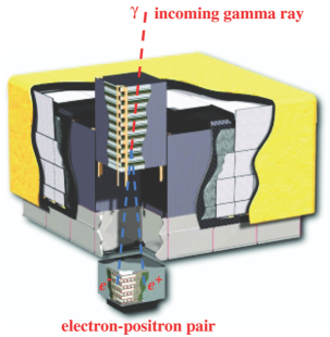
Figure 2.5: A schematic diagram of the LAT with an incident $\gamma$-ray (red line) pair-converting into an electron and positron pair (blue lines). This figure is taken from (Atwood et al. 2009).

The Fermi Gamma-ray Space telescope was launched on June 11, 2008 on a Delta II heavy launch vehicle (Atwood et al. 2009). The primary since instrument on board Fermi is the LAT, a pair-conversion telescope which detects $\gamma$-rays in the energy range from $20\,\text{MeV}$ to $>300\,\text{GeV}$ (see Figure 2.5). In addition, Fermi contains the Gamma-ray Burst Monitor (GBM), which is used to observe gamma-ray bursts (GRBs) in the energy range from $\sim 8\,\text{keV}$ to $\sim 40\,\text{MeV}$. See Meegan et al. (2009) for a description of the GBM.

2.3.1 The LAT Detector

The LAT is composed of three major subsystems: the tracker, the calorimeter, and the Anti-Coincidence Detector (ACD). Fundamentally, the detector operates by inducing an incident $\gamma$-ray to pair convert in the tracker into an electron and positron pair. The electron and position travel through the tracker and into the cesium iodide (CsI) calorimeter. The tracks and energy deposit can be used to infer the direction and energy of the incident $\gamma$-ray. Both the tracker and calorimeter are $4\times 4$ arrays, each composed of 16 modules. Each tracker tower is divided into 18 tungsten converter layers and 16 dual-silicon tracker planes. Each calorimeter module is composed of eight layers of 12 CsI crystals.

The ACD provides provides background rejection of charged particles incident on the LAT. The ACD surrounds the tracker and is composed of 89 plastic scintillator tiles ($5\times 5$ on the top and 16 on each of the sides). The ACD has a 0.9997 efficiency for detecting singly-charged particles entering the LAT. A detailed discussion of the various subsystems of the LAT can be found in (Atwood et al. 2009).

2.3.2 Performance of the LAT

The LAT has an unprecedented effective area ($\sim 9,500\,\text{cm}^{2}$), single-photon energy resolution ($\sim 10\%$), and single-photon angular resolution ($\sim 3\mbox{$.\!\!^{\circ}$}5$ at $E=100\,\text{MeV}$ and decreasing to $\lesssim 0\mbox{$.\!\!^{\circ}$}15$ for $E>10\,\text{GeV}$) (Atwood et al. 2009).

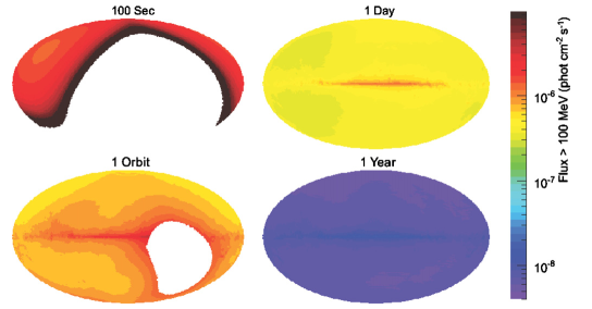
Figure 2.6: The LAT point-source sensitivity for exposures of $100\,\text{s}$, 1 orbit, $1\,\text{day}$, and $1\,\text{yr}$. This figure is from Atwood et al. (2009).

With its $2.4\,\text{sr}$ field of view, Fermi can observe the entire sky almost uniformly every $\sim 3\,\text{hr}$. With one year of observations, the LAT has a point-source flux sensitivity $3\times 10^{-9}($E¿100 MeV $)\text{ph}\,\text{cm}^{-2}\text{s}{-1}$ assuming a high-latitude diffuse flux of $1.5\times 10^{-5}\text{cm}^{-2}\text{s}^{-1}\text{sr}^{-1}$ ($E>100\,\text{MeV}$) Figure 2.6 plots the sensitivity for exposures of varying timescales.

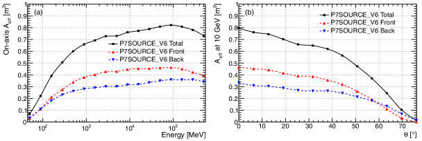
Figure 2.7: The LAT effective area (a) as a function of energy for $\gamma$-rays that are incident on the LAT perpendicularly from above and (b) as a function of incident angle for photons with an energy of $10\,\text{GeV}$. The LAT performance is computed for the P7SOURCE_V6 event classification. This figure is from Ackermann et al. (2012).

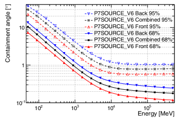
Figure 2.8: The angular resolution (68% and 95% containment radius) as a function of energy. The LAT performance is computed for the P7SOURCE_V6 event classification. This figure is from Ackermann et al. (2012).

Figure 2.9: The energy dispersion (a) as a function of energy for $\gamma$-rays that are incident on the LAT perpendicularly from above and (b) as a function of the incident angle for photons with an energy of $10\,\text{GeV}$. The LAT performance is computed for the P7SOURCE_V6 event classification. This figure is from Ackermann et al. (2012).

The effective area, point spread function (PSF), and energy dispersion are both a function of energy and of incident angle. Figure 2.7 plots the effective area as a function of energy and incident angle. Figure 2.8 plots the PSF as a function of energy. Finally, Figure 2.9 plots the energy dispersion as a function of energy and incident angle. We will describe in Chapter 4 the analysis methods used to analyze LAT data.

2.4 Pulsars and Pulsar Wind Nebulae

2.4.1 Pulsars

It is widely accepted that in the collapse of a massive star, a large amount of ejecta is released as a supernova powering a supernova remnant (SNR) and that much of the remaining mass collapses into a neutron star (Baade & Zwicky 1934).

Pulsars were first discovered observationally in 1967 by Jocelyn Bell Burnell and Antony Hewish (Hewish et al. 1968). We note in that pulsars had been previously observed by the air force (Brumfiel 2007). Even before the discovery, Pacini (1967) had predicted the existence of neutron stars (NSs). Shortly following the 1967 discovery, Gold (1968) and Pacini (1968) argued the connection between pulsars and rotating NSs.

The discovery of many more pulsars came quickly. In 1968, and the Vela pulsar (Large et al. 1968) and the Crab pulsar (Staelin & Reifenstein 1968) were discovered. The first pulsar observed at optical frequencies was the Crab (Cocke et al. 1969). In the same year, the first X-ray pulsations were discovered from the same source from an X-ray detector on a rocket. The discovery was carried out almost concurrently by a group at the Naval Research Laboratory (NRL) (Fritz et al. 1969) and at the Massachusetts Institute of Technology (MIT) (Bradt et al. 1969). Using proportional counters, these experiments showed that the pulsed emission from the Crab extended to X-ray energies and that, for this source, the X-rays emission was a factor $>100$ more energetic than the observed visible emission.

From these early sources, pulsar physics has blossomed into a vast field. In the on-line Australia Telescope National Facility (ATNF) catalog, there are currently over 2,200 pulsars (Manchester et al. 2005).

As was discussed in Section 2.2, the first pulsar was observed in $\gamma$-ray in 1970 (Kniffen & Fichtel 1970). Observations by EGRET brought the total number of $\gamma$-ray-detected pulsars to six (Nolan et al. 1996). Fermi has vastly expanded the number of pulsars detected in $\gamma$-rays and we will discuss these observations in Section 2.5.3

2.4.2 Pulsar Wind Nebulae

A PWN is a diffuse nebula of shocked relativistic particles that surrounds and is powered by an accompanying pulsar. PWNe have been observed long before the discovery of pulsars, but the pulsar/PWN connection was not made until after the detection of pulsars.

The most famous PWNe is the Crab nebula, associated with the Crab pulsar. The Crab supernova (SN) (SN 1054) was observed by Chinese astrologers in 1054 AD Hester (2008). It was also likely observed in Japan, Europe, by Native Americans, and in the Arab world (see Collins et al. 1999, and references therein).

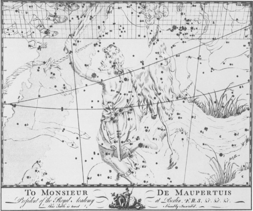
Figure 2.10: The Orion plate from Bevis’ book Uranographia Britannica. The Crab nebula can be found on the horn of Taurus the Bull on the top of the figure and the source is marked by a cloudy symbol. This figure was reproduced from Ashworth (1981).

The Crab nebula, in the remains of SN 1054, was first discovered in 1731 by physician and amateur astronomer John Bevis. This source was going to be published in his sky atlas Uranographia Britannica, but the work was never published because his publisher filed for bankruptcy in 1750. Figure 2.10 shows Beavis’ plate containing the Crab nebula. A detailed history of John Bevis’ work can be found in Ashworth (1981). The Crab Nebulae was famously included in Charles Messier’s catalog as M1 in 1758 Hester (2008).

In 1921, Lampland (1921) observed motions and changes in brightness of parts of the nebula. In the same year, Duncan (1921) observed that the entire nebula was expanding. Also in the same year Knut Lundmark proposed a connection between the Crab Nebula and the 1054 supernova (Lundmark 1921). In 1942, Mayall & Oort (1942) connected improved historical observations with a detailed study of the historical record to unmistakably connect the Crab nebula to SN 1054.

Radio emission from the Crab nebula was first detected in 1949 (Bolton et al. 1949). The synchrotron hypothesis for the observed emission was first proposed by Shklovskii (1953), and quickly confirmed by optical polarization observations (Dombrovsky 1954). X-rays from the object were first detected by Bowyer et al. (1964). As was discussed in Section 2.2, the Crab pulsar was discovered in 1968. In the discovery paper, the SN, PWN, NS connection was proposed (Staelin & Reifenstein 1968).

The synchrotron and IC model of the Crab nebula predicting observable VHE emission was first proposed by Gould & Burbidge (1965), and improved in Rieke & Weekes (1969) and Grindlay & Hoffman (1971). As was discussed in Section 2.2, $\gamma$-rays from the Crab nebula were first observed by Nolan et al. (1993). VHE emission from the Crab nebula by an Imaging air Cherenkov detector (IACT) was first observed by Weekes et al. (1989).

PWNe are commonly observed to surround pulsars. Some of the famous PWNe include Vela$-$X surrounding the Vela pulsar (first observed by Rishbeth 1958), 3C 58 (Slane et al. 2004), and MSH 15$-$52 (Seward & Harnden 1982). There are now over 50 sources identified as being PWNe both inside our galaxy and in the Large Magellanic Cloud (LMC) Kaspi et al. (2006). In addition, many PWN have been detected at VHE energies. As of April 2013, the TeVCat includes 31 VHE sources classified as PWNe. We will discuss these VHE PWN in Chapter 8.

2.5 Sources Detected by Large Area Telescope

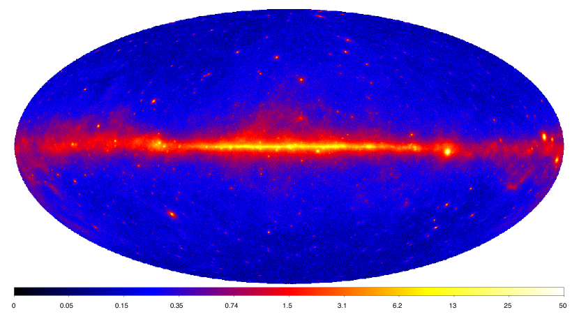
Figure 2.11: An Aitoff projection map of the $\gamma$-ray sky observed by the LAT with a 2 year exposure. This map is integrated in the energy range from $100\,\text{MeV}$ to $10\,\text{GeV}$ in units of $10^{-7}\text{erg}\,\text{cm}^{-2}\text{s}^{-1}\text{sr}^{-1}$. This figure is from Nolan et al. (2012).

Figure 2.11 shows a map of the $\gamma$-ray sky observed by the LAT with two years of data. One can clearly observed a strongly-structured anisotropic component of the $\gamma$-ray emission coming from the galaxy. In addition, many individual sources of $\gamma$-rays can be viewed. In Section 2.5.1, we discuss the Galactic diffuse and isotropic $\gamma$-ray background. In Section 2.5.2, we discuss the second Fermi catalog (2FGL), a catalog of point-like sources detected by the LAT. In Section 2.5.3, we discuss the second Fermi pulsar catalog (2PC), a catalog of pulsars detected by the LAT. Finally, in Section 2.5.4 we discuss PWNe detected by the LAT.

2.5.1 The Galactic Diffuse and Isotropic Gamma-ray Background

The structured Galactic diffuse $\gamma$-ray emission in our galaxy is caused by The interaction of cosmic-ray electrons and protons with the gas in our Milky Way (through the ${\pi}^{0}$ and bremsstrahlung process) and with Galactic radiation fields (through the IC process).

Much work has gone into theoretically modeling this diffuse $\gamma$-ray emission. The most advanced theoretical model of the Galactic emission is GALPROP (Strong & Moskalenko 1998; Moskalenko & Strong 2000). In addition, significant work has gone into comparing these models to the observed $\gamma$-ray intensity distribution observed by the LAT (Abdo et al. 2009b; Ackermann et al. 2012).

In addition to the Galactic diffuse background, the LAT observes an isotropic component to the $\gamma$-ray distribution. This emission is believed to be a composite of unresolved extragalactic point-like sources as well as a residual charged-particle background. Abdo et al. (2010d) presents detailed measurements of the isotropic background observed by the LAT.

The GALPROP predictions for the $\gamma$-ray background are not accurate enough for the analysis of point-like and $\sim 1^{\circ}$ large extended sources. Therefore, an improved data-driven model of the Galactic diffuse background has been devised where components of the GALPROP model are fit to the observed $\gamma$-ray emission. This data-driven model is described in Nolan et al. (2012).

2.5.2 The Second Fermi Catalog

Using 2 years of observations, the LAT collaboration produced a list of 1873 $\gamma$-ray-emitting sources detected in the $100\,\text{MeV}$ to $100\,\text{GeV}$ energy range (Nolan et al. 2012). Primarily, the catalog assumed sources to be point like. But twelve previously-published sources were included as being spatially extended with the spatial model taken from prior publications.

Of these 1873 sources, 127 were firmly identified with a multiwavelength counterpart. A source is only firmly identified if it meets one of three criteria. First, it can have periodic variability (pulsars and high-mass binaries). Second, it could have a matching spatial morphology (SNRs and PWNe). Finally, it could have correlated variability (active galactic nucleus (AGN)). In total, 2FGL firmly identified 83 pulsars, 28 AGNs, 6 SNRs, 4 high-mass binaries (HMBs), 3 PWNe, 2 normal galaxies, and one nova Nolan et al. (2012).

In addition, 1171 sources are included in the looser criteria that they were potentially associated with a multiwavelength counterpart. Using this criteria, 86 sources are associated with pulsars, 25 with PWNe, 98 with SNRs, and 162 were flagged as being potentially spurious due to residuals included by incorrectly modeling the galactic diffuse emission.

2.5.3 The Second Fermi Pulsar Catalog

Using 3 years of data, the LAT collaboration produced the second Fermi pulsar catalog (2PC), a list of 117 pulsars significantly detected by the LAT (Abdo et al. in prep). Typically, a LAT-detected pulsar is first detected at either radio or X-ray energies. This method was used to discover 61 of the $\gamma$-ray emitting pulsars. But some pulsars are known to emit only $\gamma$-rays. These sources can be searched for blindly using $\gamma$-ray data. This method was used to detect 36 pulsars. Finally, in the third method, the positions of unidentified LAT sources which could potentially be associated with pulsars. These regions are often searched for in radio to look for pulsar emission. This method has lead to the detection of 20 new millisecond pulsars (MSPs). In total 2PC detected 42 radio-loud pulsars, 35 radio-quiet pulsars, and 40 $\gamma$-ray MSPs.

2.5.4 Pulsar Wind Nebulae Detected by Large Area Telescope

In addition to detecting over 100 pulsars, the LAT has detected several PWNe. In situations where the PWNe has an associated LAT-detected pulsar, typically the spectral analysis of the PWN is performed during times in the pulsar phase where the pulsar emission is at a minimum. For some pulsars, such as 1825 1825HESS J1825$-$137 1640HESS J1640$-$465 1837HESS J1837$-$069 1632HESS J1632$-$478 1614HESS J1614$-$518 1616HESS J1616$-$508 1119HESS J1119$-$614 1303HESS J1303$-$631 1420HESS J1420$-$607 1841HESS J1841$-$055 1356HESS J1356$-$645 1023HESS J1023$-$575 1848HESS J1848$-$018 1514HESS J1514$-$591 1857HESS J1857$+$026 1708HESS J1708$-$443 1804HESS J1804$-$216 1634HESS J1634$-$472 1018HESS J1018$-$589 1507HESS J1507$-$622 1834HESS J1834$-$087 [], there is no associated LAT-detected pulsar and the spectral analysis can be performed without cutting on pulsar phase.

Crab

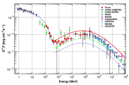
Figure 2.12: The SED of the Crab nebula observed by the LAT as well as several other instruments. This figure is from Abdo et al. (2010e).

Observations of the Crab nebula by the LAT provided detailed spectral resolution of Crab’s spectrum Abdo et al. (2010e). The Crab nebula shows a very strong spectral break in the LAT energy band, and the $\gamma$-ray emission is interpreted as being the combination of a synchrotron component at low energy and an IC component at high energy.

In addition, $\gamma$-ray emission from the Crab nebula has been observed to be variability in time and have flaring periods (Abdo et al. 2011a). The Crab was observed to have an extreme flare in 2011 (Buehler et al. 2012). This variability is challenging to understand given conventional models of PWN emission.

Vela$-$X

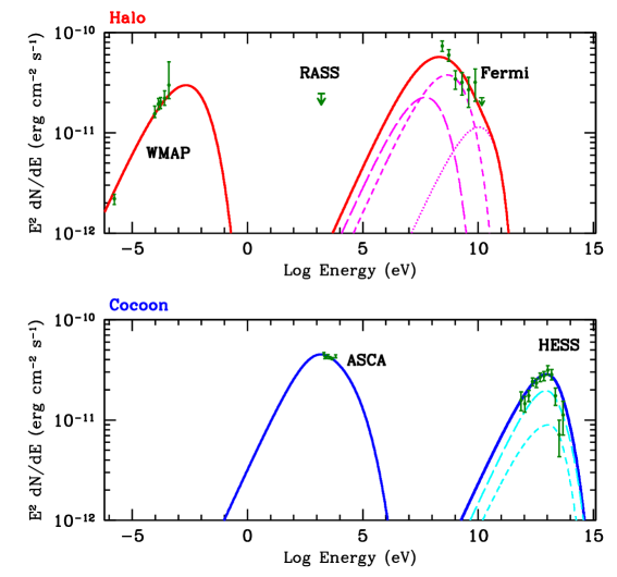
Figure 2.13: The SED of Vela$-$X observed at radio, x-ray, $\gamma$-ray, and VHE energies. The emission was suggested by (Abdo et al. 2010) to be driven by two pollutions of electrons. In this model, the lower-energy electron population powers the radio and $\gamma$-ray emission adn the higher-energy electron population powers the x-ray and VHE emission. This figure is from Abdo et al. (2010).

Vela$-$X is a PWN powered by the Vela pulsar. It was first observed by Rishbeth (1958). It was observed at VHE energies by Aharonian et al. (2006d) and at GeV energies by AGILE (Pellizzoni et al. 2010). The detailed multiwavelength spectra of Vela$-$X is plotted in Figure 2.13. Based upon the morphological and spectral disconnect between the GeV and TeV emission, (Abdo et al. 2010) argued that emission was not consistent with a single population of accelerated electrons. They suggested instead that the emission comes instead from two populations of electrons.

MSH 15$-$52

SNR (MSH 15$-$52 Caswell et al. 1981) is commonly associated with 1509 1823PSR B1823$-$13 1509PSR B1509$-$58 [] (Seward & Harnden 1982). A diffuse nebula was observed surrounding the pulsar (Seward & Harnden 1982), adn interpreted as an PWN Trussoni et al. (1996). The PWN was detected at VHE energies by Aharonian et al. (2005a) and at GeV energies by Abdo et al. (2010a)

1825 1825HESS J1825$-$137 1640HESS J1640$-$465 1837HESS J1837$-$069 1632HESS J1632$-$478 1614HESS J1614$-$518 1616HESS J1616$-$508 1119HESS J1119$-$614 1303HESS J1303$-$631 1420HESS J1420$-$607 1841HESS J1841$-$055 1356HESS J1356$-$645 1023HESS J1023$-$575 1848HESS J1848$-$018 1514HESS J1514$-$591 1857HESS J1857$+$026 1708HESS J1708$-$443 1804HESS J1804$-$216 1634HESS J1634$-$472 1018HESS J1018$-$589 1507HESS J1507$-$622 1834HESS J1834$-$087 []

1825 1825HESS J1825$-$137 1640HESS J1640$-$465 1837HESS J1837$-$069 1632HESS J1632$-$478 1614HESS J1614$-$518 1616HESS J1616$-$508 1119HESS J1119$-$614 1303HESS J1303$-$631 1420HESS J1420$-$607 1841HESS J1841$-$055 1356HESS J1356$-$645 1023HESS J1023$-$575 1848HESS J1848$-$018 1514HESS J1514$-$591 1857HESS J1857$+$026 1708HESS J1708$-$443 1804HESS J1804$-$216 1634HESS J1634$-$472 1018HESS J1018$-$589 1507HESS J1507$-$622 1834HESS J1834$-$087 [] is an extended ($\sim 0\mbox{$.\!\!^{\circ}$}5$) VHE sources first detected during the the High Energy Stereoscopic System (H.E.S.S.) survey of the inner galaxy (Aharonian et al. 2006e). It was interpreted by Aharonian et al. (2005c) as being a PWN powered by 1826 1119PSR J1119$-$6127 1301PSR J1301$-$6305 1023PSR J1023$-$5746 1420PSR J1420$-$6048 1838PSR J1838$-$0537 1826PSR J1826$-$1334 1856PSR J1856$+$0245 [] (also known as 1823 1823PSR B1823$-$13 1509PSR B1509$-$58 [], Clifton et al. 1992). Surrounding the pulsar is a diffuse $\sim 5^{\prime}$ nebula (Finley et al. 1996). The large size difference can be understood in terms of the different lifetimes for the synchrotron-emitting and IC-emitting electrons (Aharonian et al. 2006e).

This source was subsequently detected by Grondin et al. (2011) at GeV energies. Interestingly, the VHE emission from 1825 1825HESS J1825$-$137 1640HESS J1640$-$465 1837HESS J1837$-$069 1632HESS J1632$-$478 1614HESS J1614$-$518 1616HESS J1616$-$508 1119HESS J1119$-$614 1303HESS J1303$-$631 1420HESS J1420$-$607 1841HESS J1841$-$055 1356HESS J1356$-$645 1023HESS J1023$-$575 1848HESS J1848$-$018 1514HESS J1514$-$591 1857HESS J1857$+$026 1708HESS J1708$-$443 1804HESS J1804$-$216 1634HESS J1634$-$472 1018HESS J1018$-$589 1507HESS J1507$-$622 1834HESS J1834$-$087 [] was observed to have an energy-dependent morphology, with the size decreasing with increasing energy (Aharonian et al. 2006c). This can be explained by the IC emission model if the electron injection decreases with time.

1640 1825HESS J1825$-$137 1640HESS J1640$-$465 1837HESS J1837$-$069 1632HESS J1632$-$478 1614HESS J1614$-$518 1616HESS J1616$-$508 1119HESS J1119$-$614 1303HESS J1303$-$631 1420HESS J1420$-$607 1841HESS J1841$-$055 1356HESS J1356$-$645 1023HESS J1023$-$575 1848HESS J1848$-$018 1514HESS J1514$-$591 1857HESS J1857$+$026 1708HESS J1708$-$443 1804HESS J1804$-$216 1634HESS J1634$-$472 1018HESS J1018$-$589 1507HESS J1507$-$622 1834HESS J1834$-$087 []

The VHE source 1640 1825HESS J1825$-$137 1640HESS J1640$-$465 1837HESS J1837$-$069 1632HESS J1632$-$478 1614HESS J1614$-$518 1616HESS J1616$-$508 1119HESS J1119$-$614 1303HESS J1303$-$631 1420HESS J1420$-$607 1841HESS J1841$-$055 1356HESS J1356$-$645 1023HESS J1023$-$575 1848HESS J1848$-$018 1514HESS J1514$-$591 1857HESS J1857$+$026 1708HESS J1708$-$443 1804HESS J1804$-$216 1634HESS J1634$-$472 1018HESS J1018$-$589 1507HESS J1507$-$622 1834HESS J1834$-$087 [] (Aharonian et al. 2006e) is spatially-coincident with 338.3 284.3SNR G284.3$-$1.8 320.4SNR G320.4$-$1.2 338.3SNR G338.3$-$0.0 8.7SNR G8.7$-$0.1 [] (Shaver & Goss 1970). X-ray observations by XMM-Newton uncovered a spatially-coincident X-ray nebula and within it a point-like source Funk et al. (2007). This point-like source is believed to be a neutron star powering the PWN, but pulsations have not yet been detected from it. Slane et al. (2010) discovered an associated GeV source.

1857 1825HESS J1825$-$137 1640HESS J1640$-$465 1837HESS J1837$-$069 1632HESS J1632$-$478 1614HESS J1614$-$518 1616HESS J1616$-$508 1119HESS J1119$-$614 1303HESS J1303$-$631 1420HESS J1420$-$607 1841HESS J1841$-$055 1356HESS J1356$-$645 1023HESS J1023$-$575 1848HESS J1848$-$018 1514HESS J1514$-$591 1857HESS J1857$+$026 1708HESS J1708$-$443 1804HESS J1804$-$216 1634HESS J1634$-$472 1018HESS J1018$-$589 1507HESS J1507$-$622 1834HESS J1834$-$087 []

1857 1825HESS J1825$-$137 1640HESS J1640$-$465 1837HESS J1837$-$069 1632HESS J1632$-$478 1614HESS J1614$-$518 1616HESS J1616$-$508 1119HESS J1119$-$614 1303HESS J1303$-$631 1420HESS J1420$-$607 1841HESS J1841$-$055 1356HESS J1356$-$645 1023HESS J1023$-$575 1848HESS J1848$-$018 1514HESS J1514$-$591 1857HESS J1857$+$026 1708HESS J1708$-$443 1804HESS J1804$-$216 1634HESS J1634$-$472 1018HESS J1018$-$589 1507HESS J1507$-$622 1834HESS J1834$-$087 [] was also discovered by H.E.S.S. (Aharonian et al. 2008c) Hessels et al. (2008) suggested that 1857 1825HESS J1825$-$137 1640HESS J1640$-$465 1837HESS J1837$-$069 1632HESS J1632$-$478 1614HESS J1614$-$518 1616HESS J1616$-$508 1119HESS J1119$-$614 1303HESS J1303$-$631 1420HESS J1420$-$607 1841HESS J1841$-$055 1356HESS J1356$-$645 1023HESS J1023$-$575 1848HESS J1848$-$018 1514HESS J1514$-$591 1857HESS J1857$+$026 1708HESS J1708$-$443 1804HESS J1804$-$216 1634HESS J1634$-$472 1018HESS J1018$-$589 1507HESS J1507$-$622 1834HESS J1834$-$087 [] is a PWN powered by 1856 1119PSR J1119$-$6127 1301PSR J1301$-$6305 1023PSR J1023$-$5746 1420PSR J1420$-$6048 1838PSR J1838$-$0537 1826PSR J1826$-$1334 1856PSR J1856$+$0245 []. 1857 1825HESS J1825$-$137 1640HESS J1640$-$465 1837HESS J1837$-$069 1632HESS J1632$-$478 1614HESS J1614$-$518 1616HESS J1616$-$508 1119HESS J1119$-$614 1303HESS J1303$-$631 1420HESS J1420$-$607 1841HESS J1841$-$055 1356HESS J1356$-$645 1023HESS J1023$-$575 1848HESS J1848$-$018 1514HESS J1514$-$591 1857HESS J1857$+$026 1708HESS J1708$-$443 1804HESS J1804$-$216 1634HESS J1634$-$472 1018HESS J1018$-$589 1507HESS J1507$-$622 1834HESS J1834$-$087 [] was also detected by the LAT.

1023 1825HESS J1825$-$137 1640HESS J1640$-$465 1837HESS J1837$-$069 1632HESS J1632$-$478 1614HESS J1614$-$518 1616HESS J1616$-$508 1119HESS J1119$-$614 1303HESS J1303$-$631 1420HESS J1420$-$607 1841HESS J1841$-$055 1356HESS J1356$-$645 1023HESS J1023$-$575 1848HESS J1848$-$018 1514HESS J1514$-$591 1857HESS J1857$+$026 1708HESS J1708$-$443 1804HESS J1804$-$216 1634HESS J1634$-$472 1018HESS J1018$-$589 1507HESS J1507$-$622 1834HESS J1834$-$087 []

The VHE source 1023 1825HESS J1825$-$137 1640HESS J1640$-$465 1837HESS J1837$-$069 1632HESS J1632$-$478 1614HESS J1614$-$518 1616HESS J1616$-$508 1119HESS J1119$-$614 1303HESS J1303$-$631 1420HESS J1420$-$607 1841HESS J1841$-$055 1356HESS J1356$-$645 1023HESS J1023$-$575 1848HESS J1848$-$018 1514HESS J1514$-$591 1857HESS J1857$+$026 1708HESS J1708$-$443 1804HESS J1804$-$216 1634HESS J1634$-$472 1018HESS J1018$-$589 1507HESS J1507$-$622 1834HESS J1834$-$087 [] was discovered in the region of the young stellar cluster Westerlund 2 Aharonian et al. (2007a). This same source was subsequently detected by the LAT in the off-peak region surrounding 1023 1119PSR J1119$-$6127 1301PSR J1301$-$6305 1023PSR J1023$-$5746 1420PSR J1420$-$6048 1838PSR J1838$-$0537 1826PSR J1826$-$1334 1856PSR J1856$+$0245 [] (Ackermann et al. 2011a). H.E.S.S. Collaboration et al. (2011e) proposed that the emission could either be due to an PWNe or due to hadronic interactions of cosmic rays accelerated in the open stellar cluster interacting with molecular clouds.

2.6 Radiation Processes in Gamma-ray Astrophysics

Nonthermal radiation observed from astrophysical sources is typically believed to originate in through synchrotron radiation, IC upscattering, and the decay of neutral ${\pi}^{0}$ particles. We will discuss these processes in Section 2.6.1, Section 2.6.2, and Section 2.6.3 respectively.

2.6.1 Synchrotron

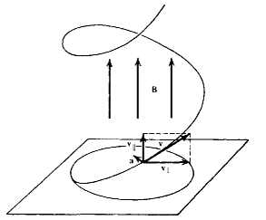
Figure 2.14: In synchrotron radiation, charged particles spiral along magnetic filed lines, radiating photons as they accelerate. This figure is from Rybicki & Lightman (1979).

The synchrotron radiation processes is observed when charged particles spiral around magnetic field lines. This process is illustrated in Figure 2.14. This emission is discussed thoroughly in Blumenthal & Gould (1970) and Rybicki & Lightman (1979). In what follows, we adopt the notation from Houck & Allen (2006).

A charged particle of mass $m$ and charge $q$ in a magnetic field of strength $\boldsymbol{B}$ will experience an electromagnetic force:

$$\frac{\text{d}}{\text{d}t}(\gamma m\boldsymbol{v})= \frac{q}{c}\boldsymbol{v}\!\boldsymbol{\times}\!\boldsymbol{B}.$$ (2.1)

This force will cause a particle to accelerate around the magnetic field lines, radiating due to maxwell’s equations. The power emitted at a frequency $\nu$ by one of these particles is

$$P_{\text{emitted}}(\nu)=\frac{\sqrt{3}q^{3}B\sin\alpha}{mc^{2}}F(\nu/\nu_{c}),$$ (2.2)

where $\alpha$ is the angle between the particle’s velocity vector and the magnetic field vector. Here,

$$F(x)\equiv x\int_{x}^{\infty}K_{\tfrac{5}{3}}(\xi)d\xi,$$ (2.3)

and

$$\nu_{c}=\frac{3qB\gamma^{2}}{4\pi mc}\sin\alpha\equiv\nu_{0}\gamma^{2}\sin\alpha$$ (2.4)

Because power is inversely-proportional to mass, synchrotron radiation is predominatly from electrons.

Now, we assume a population of particles and compute the total observed emission. We say that $N(p,\alpha)$ is the number of particles per unit momentum and solid angle with a momentum $p$ and pitch angle $\alpha$. We find the total power emitted by integrating over particle momentum and distribution

$$\frac{\text{d}W}{\text{d}t}=\int\text{d}p\int\text{d}\vec{\Omega}P_{\text{emitted}}(\nu)N(p,\alpha)$$ (2.5)

If we assume the pitch angles of the particles to be isotropically distributed and, including Equation 2.2, we find that the number of photons emitted per unit energy and time is

$$\frac{\text{d}N}{\text{d}\omega\text{d}t}=\frac{\sqrt{3}q^{3}B}{hm_{e}c^{2}\omega}\int\text{d}pN(p)R\left(\frac{\omega}{\omega_{0}\gamma^{2}}\right)$$ (2.6)

where

$$R(x)\equiv\frac{1}{2}\int_{0}^{\pi}\text{d}\alpha\sin^{2}\alpha F\left(\frac{x}{\sin\alpha}\right)$$ (2.7)

It is typical in astrophysics to assume a a power-law distribution of electrons:

$$N(p)\text{d}p=\kappa p^{-\gamma}\text{d}p.$$ (2.8)

For a power-law distribution of photons integrated over pitch angle, we find the total power emitted to me

$$P_{\text{tot}}(\omega)\propto\kappa B^{(p+1)/2}\omega^{-(p-1)/2}.$$ (2.9)

See, Rybicki & Lightman (1979) or Longair (2011) for a full derivation. This shows that, assuming a power-law electron distribution, the electron spectral index can be related to the photon spectral index.

2.6.2 Inverse Compton

Normal Compton scattering involves a photon colliding with a free electron and transferring energy to it. In IC scattering, a high-energy electron interacts with a low-energy photon imparting energy to it. This process occurs when highly-energetic electrons interact with a dense photon field.

The derivation of IC emission requires a quantum electrodynamical treatment. It was first derived by Klein & Nishina (1929). In what follows, we follow the notational convention of Houck & Allen (2006). We assume a population of relativistic ($\gamma\gg 1$) electrons written as $N(p)$ which is contained inside isotropic photon distribution with number density $n(\omega_{i})$.

The distribution of photons emitted by IC scatter is written as

$$\frac{\text{d}N}{\text{d}\omega\text{d}t}=c\int d\omega_{i}n(\omega_{i})\int_{p_{\text{min}}}^{\infty}dpN(p)\sigma_{\text{KN}}(\gamma,\omega_{i},\omega)$$ (2.10)

where $\omega$ is the outgoing photon energy written in units of the electron rest mass energy, $\omega\equiv h\nu/(m_{e}c^{2})$, and $\sigma_{\text{KN}}$ is the Klein-Nishina cross section:

$$\sigma_{\text{KN}}(\gamma,\omega_{i},\omega)=\frac{2\pi r_{0}^{2}}{\omega_{i}\gamma^{2}}\left[1+q-2q^{2}+2q\ln q+\frac{\tau^{2}q^{2}(1-q)}{2(1+\tau q)}.\right]$$ (2.11)

Here,

$$q\equiv\frac{\omega}{4\omega_{i}\gamma(\gamma-\omega)},$$ (2.12)

$\tau\equiv 4\omega_{i}\gamma$, and $r_{0}=e^{2}/(m_{e}c^{2})$ is the classical electron radius. The threshold electron Lorentz factor is

$$\gamma_{\text{min}}=\frac{1}{2}\left(\omega+\sqrt{\omega^{2}+\frac{\omega}{\omega_{i}}}\right)$$ (2.13)

Often, IC emission happens when an accelerated power-law distribution of electrons interacts with a thermal photon distribution

$$n(\omega_{i})=\frac{1}{\pi^{2}\lambda^{3}}\frac{\omega_{i}^{2}}{e^{\omega_{i}/\Theta}-1}$$ (2.14)

where $\lambda=\hbar/(m_{e}c)$ and $\Theta=kT/(m_{e}c^{2})$. Often, the target photon distribution is the cosmic microwave background (CMB), with $T=2.725\,\text{K}$.

2.6.3 Bremsstrahlung

Bremsstrahlung radiation is composed of electron-electron and electron-ion interactions. In either case, we assume a differential spectrum of accelerated electrons $N_{e}(E)$ that interacts with a target density of electrons ($n_{e}$) or ions ($n_{Z}$).

$$\frac{\text{d}N}{\text{d}E\text{d}t}=n_{e}\int\text{d}EN_{e}(E)v_{e}\frac{\text{d}\sigma_{ee}}{\text{d}E}+n_{Z}\int\text{d}EN_{e}(E)v_{e}\frac{\text{d}\sigma_{eZ}}{\text{d}E}$$ (2.15)

Here, $v_{e}$ is the velocity of the electron, and $\sigma_{ee}$ and $\sigma_{eZ}$ are the electron-electron and electron-ion cross sections. The actual formulas for $\text{d}\sigma_{ee}/\text{d}E$ and $\text{d}\sigma_{eZ}/\text{d}E$ are quite involved. The electron-electron cross section was worked out in Haug (1975). The electron-ion cross section is called the Bethe-Heitler cross-section and is worked out in the Born approximation in Heitler (1954) and Koch & Motz (1959). A more accurate relativistic correction to this formula is given in Haug (1997). We refer to Houck & Allen (2006) for a detailed numerical implementation of these formulas.

2.6.4 Pion Decay

Neutral ${\pi}^{0}$ decay occurs when highly-energetic protons interact with thermal protons. This emission happens when protons decay into neutral pions through $pp\rightarrow{\pi}^{0}+X$ and the ${\pi}^{0}$ subsequently decay through ${\pi}^{0}\rightarrow 2\gamma$. The gamma-ray emission from neutral pion decay can be computed as

$$\frac{\text{d}N}{\text{d}E\text{d}t}=n_{H}\int\text{d}Ev_{p}N_{p}(E)\frac{\text{d}\sigma_{pp}}{\text{d}E}$$ (2.16)

Here, $N_{p}(E)$ is the differential proton distribution, $\text{d}\sigma_{pp}/\text{d}E$ is $\gamma$-ray cross section from proton-proton interactions, and $n_{H}$ is the target hydrogen density. The computation of $\text{d}\sigma_{pp}/\text{d}E$ is rather involved. Typically, people employ a parameterization of the calculations performed by Kamae et al. (2006).

Chapter 3 The Pulsar/Pulsar Wind Nebula System

3.1 Neutron Star Formation

As was discussed in Section 2.4, pulsars, PWNe, and supernova remnants are all connected through the death of a star. When a star undergoes a supernova, the ejecta forms a supernova remnant. If the remaining stellar core has a mass above the Chandrasekhar limit, then the core’s electron degeneracy pressure cannot counteract the core’s gravitational force and the core will collapse into a NS. The Chandrasekhar mass limit can be approximated as (Chandrasekhar 1931)

$$M_{\text{Ch}}\approx\frac{3\sqrt{2\pi}}{8}\left(\frac{\hbar c}{G}\right)^{3/2}\left[\left(\frac{Z}{A}\right)\frac{1}{m_{\text{H}}^{2}}\right],$$ (3.1)

where $\hbar$ is the reduced Planck constant, $c$ is the speed of light, $G$ is the gravitational constant, $m_{\text{H}}$ is the mass of hydrogen, $Z$ is the number of protons, $A$ is the number of nucleons, and $M_{\odot}$ is the mass of the sun (Carroll & Ostlie 2006). When this formula is computed more exactly, one finds $M_{\text{Ch}}=1.44M_{\odot}$.

Because NSs are supported by neutron degeneracy pressure, the radius of a neutron star can be approximated as (Carroll & Ostlie 2006)

$$R_{\text{ns}}\approx\frac{(18\pi)^{2/3}}{10}\frac{\hbar^{2}}{GM_{\text{ns}}^{1/3}}\left(\frac{1}{m_{\text{H}}}\right)^{8/3}.$$ (3.2)

The canonical radius for NSs is $\sim 10\,\text{km}$.

In these very dense environments, the protons and electrons in the NS form into neutrons through inverse $\beta$ decay:

$$p^{+}+e^{-}\rightarrow n+\nu_{e}.$$ (3.3)

If a NS had a sufficiency large mass, the gravitational force would overpower the neutron degeneracy pressure and the object would collapse into a black hole. The maximum mass of a NS is unknown because it depends on the equation of state inside the star, but is commonly predicted to be $\sim 2.5M_{\odot}$ Recently, a pulsar with a mass of $\sim 2M_{\odot}$ was discovered (Demorest et al. 2010), constraining theories of the equation of state.

In addition to rotationally-powered pulsars, the primary class of observed pulsars, there are two additional classes of pulsars with a different emission mechanism. For accretion-powered pulsars, also called X-ray pulsars, the emission energy comes from the accretion of matter from a donor star (Caballero & Wilms 2012). They are bright and populous at X-ray energies. Magnetars have the strong magnetic field which power their emission Rea & Esposito (2011).

3.2 Pulsar Evolution

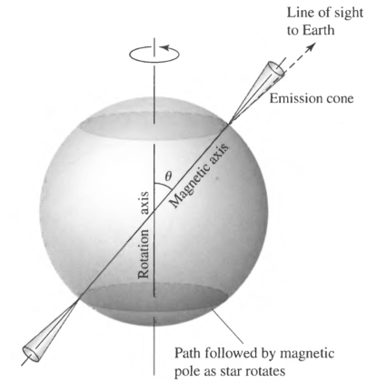
Figure 3.1: The rotating dipole model of a pulsar. This figure is taken from (Carroll & Ostlie 2006).

The simplest model of a pulsar is that it is a rotating dipole magnet with the rotation axis and the magnetic axis offset by an angle $\theta$ (see Figure 3.1). The energy output from the pulsar is assumed to come from rotational kinetic energy stored in the neutron star which is released as the pulsar spins down.

For a pulsar, both the period $P$ and the period derivative $\dot{P}=dP/dt$ can be directly observed. Except in a few MSPs which are being sped up through accretion (see for example Falanga et al. 2005)), pulsars are slowing down ($\dot{P}<0$). We write the rotational kinetic energy as

$$E_{\text{rot}}=\tfrac{1}{2}I\Omega^{2}$$ (3.4)

where $\Omega=2\pi/P$ is the angular frequency of the pulsar and $I$ is the moment of inertia. For a uniform sphere,

$$I=\frac{2}{5}MR^{2}.$$ (3.5)

Assuming a canonical pulsar (see Section 3.1), we find a canonical moment of inertia of $I=10^{45}\,\text{g}\,\text{cm}^{-2}$.

We make the connection between the pulsar’s spin-down energy and the rotational kinetic energy as $\dot{E}=-\text{d}E_{\text{rot}}/\text{d}t$. Equation 3.4 can be rewritten as

$$\dot{E}=I\Omega\dot{\Omega}.$$ (3.6)

It is believed that as the pulsar spins down, the this rotational energy is released as pulsed electromagnetic radiation and also as a wind of electrons and positrons accelerated in the magnetic field of the pulsar.

If the pulsar were a pure dipole magnet, its radiation would be described as (Gunn & Ostriker 1969)

$$\dot{E}=\frac{2B^{2}R_{\text{NS}}^{6}\Omega^{4}\sin^{2}\theta}{3c^{3}}.$$ (3.7)

Combining equations Equation 3.6 and Equation 3.7, we find that for a pure dipole magnet,

$$\dot{\Omega}\propto\Omega^{3}.$$ (3.8)

In the few situations where this relationship has been conclusively measured, this relationship does not hold (See Espinoza et al. 2011, and references therein). We generalize Equation 3.8 as:

$$\dot{\Omega}\propto\Omega^{n}$$ (3.9)

where $n$ is what we call the breaking index. We solve Equation 3.9 for $n$ by taking the derivative:

$$n=\frac{\Omega\ddot{\Omega}}{\dot{\Omega}^{2}}$$ (3.10)

The breaking index is hard to measure due to timing noise and glitches in the pulsar’s phase. To this date, it has been measured in eight pulsars Espinoza et al. (2011), and in all situations $n<3$. This suggests that there are additional processes besides magnetic dipole radiation that contribute to the energy release (Blandford & Romani 1988).

Equation 3.9 is a Bernoulli differential equation which can be integrated to solve for time:

$$T=\frac{P}{(n-1)|\dot{P}|}\left(1-\left(\frac{P_{0}}{P}\right)^{(n-1)}\right)$$ (3.11)

For a canonical $n=3$ pulsars which is relatively old $P_{0}\ll P$, we obtain what is called the characteristic age of the pulsar:

$$\tau_{c}=P/2\dot{P}.$$ (3.12)

Using Equation 3.6 and Equation 3.8, we can solve for the spin-down evolution of the pulsar as a function of time (Pacini & Salvati 1973):

$$\dot{E}(t)=\dot{E}_{0}\left(1+\frac{t}{\tau_{\text{dec}}}\right)^{-\frac{(n+1)}{(n-1)}}.$$ (3.13)

Here,

$$\tau_{\text{dec}}\equiv\frac{P_{0}}{(n-1)|\dot{P}_{0}|}.$$ (3.14)

Equation 3.6, Equation 3.11, and Equation 3.13 show us that given the current period, period derivative, and breaking index, we can calculate the pulsar’s age and energy-emission history.

In a few situations, the pulsar’s age is well known and the breaking index can be measured, so $P_{0}$ can be inferred. See Kaspi & Helfand (2002) for a review of the topic. For other sources, attempts have been made to infer the initial spin-down age based on the dynamics of an associated SNR/PWN (van der Swaluw & Wu 2001).

Finally, if we assume dipole radiation is the only source of energy release, we can combine equation Equation 3.6 and Equation 3.7 to solve for the magnetic field:

$$B=\sqrt{\frac{3Ic^{3}}{8\pi^{2}R_{\text{NS}}^{6}\sin^{2}\theta}P\dot{P}}=3.2\times 10^{19}\sqrt{P\dot{P}}\,\text{G}$$ (3.15)

where in the last step we assumed the canonical values of $I=10^{45}\,\text{g}\,\text{cm}^{-2}$, $R_{\text{NS}}=10\,\text{km}$, $\theta=90^{\circ}$, and we assume that $P$ is measured in units of seconds. For example, for the Crab nebula, $P\approx 33\,\text{ms}$ (Staelin & Reifenstein 1968) and $\dot{P}\approx 36\,\text{ns}$ per day (Richards & Comella 1969) so $B\approx 10^{12}\,\text{G}$.

3.3 Pulsar Magnetosphere

The basic picture of a pulsar magnetosphere was first presented in Goldreich & Julian (1969). The magnetic dipole of the rotating NS creates a quadrupole electric field.

The potential generated by this field is given as (Goldreich & Julian 1969):

$$\Delta\Phi=\frac{B\Omega^{2}R_{\text{NS}}^{2}}{2c^{2}}\approx 6\times 10^{12}\left(\frac{B}{10^{12}\,\text{G}}\right)\left(\frac{R_{\text{NS}}}{10\,\text{km}}\right)^{3}\left(\frac{P}{1\,\text{s}}\right).$$ (3.16)

For NSs, this potential produces a magnetic field that is much larger than the gravitational force and acts as a powerful particle accelerators.

Pulsars typically release only a small percent of their overall energy budget as pulsed emission. The efficiency of converting spin-down energy into pulsed $\gamma-$rays is typically $\sim$ 0.1% to 10% (Abdo et al. 2010e). For example, the Crab nebulae is estimated to release 0.1% of it’s spin-down energy as pulsed $\gamma$-rays (Abdo et al. 2010e). Typically, the energy released as radio and optical photons is much less. The optical flux of the Crab is a factor of $\sim 100$ smaller (Cocke et al. 1969) and the radio flux is a factor of $\sim 10^{4}$ smaller. Therefore, the vast majority of the energy output of the pulsar is carried away as a pulsar wind, which will be described in the next section.

Figure 3.2: The magnetosphere for a rotating pulsar. The pulsar is on the bottom left of the plot. This figure is from Goldreich & Julian (1969).

Figure 3.2 shows a schematic diagram of this magnetosphere. It is commonly believed that the radio emission from pulsars originates within 10% of the light cylinder radius (see Kijak & Gil 2003, and references therein)

On the other hand, there is still much debate about the location of the $\gamma$-ray emission. Three locations have been proposed. In the polar cap (PC) model, the $\gamma$-ray emission arises from within one stellar radius (Daugherty & Harding 1996). This model was disfavored based upon the predicted $\gamma$-ray spectrum (Abdo et al. 2009c). In the outer gap (OG) model, $\gamma$-ray emission is predicted near the pulsar’s light cylinder (Cheng et al. 1986; Romani 1996). Finally, in the two pole caustic (TPC) model, the $\gamma$-ray emission comes from an intermediate region in the pulsar magnetosphere (Dyks & Rudak 2003; Muslimov & Harding 2004) Much work has gone into comparing the TPC and OG models in the context of detailed LAT observations of $\gamma$-ray pulsars (See for example Watters & Romani 2011; Romani et al. 2011).

3.4 Pulsar Wind Nebulae Structure

The basic picture of PWNe comes from Rees & Gunn (1974) and Kennel & Coroniti (1984b). More sophisticated models have emerged over the years. See, for example, Gelfand et al. (2009) and references therein.

The wind ejected from the pulsar’s magnetosphere is initially cold which means that it flows radially out from the pulsar. This unshocked pulsar wind only emits radiation through IC scattering (Bogovalov & Aharonian 2000). This pulsar wind forms a bubble as it presses into the SNR and forms a termination shock where the particle wind is further accelerated.

As the wind leaves the magnetosphere, it is believed to be dominated by the energy carried off in electromagnetic fields (the pointing flux $F_{E\times B}$). The rest of the energy is released as a particle flux ($F_{\text{particle}}$). We define the magnetization of the pulsar wind as

$$\sigma=\frac{F_{E\times B}}{F_{\text{particle}}}$$ (3.17)

Outside the pulsar light curve, typically $\sigma>10^{4}$, but at the termination shock typical values for $\sigma$ are $\lesssim 0.01$ (Kennel & Coroniti 1984a). The cause of this transition is uncertain (Gaensler & Slane 2006).

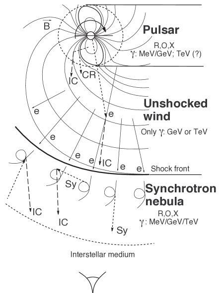
Figure 3.3: The regions of emission in a pulsar/PWN system. This figure shows (top) the pulsar’s magnetosphere, (middle), the unshocked pulsar wind and (bottom) the shocked pulsar wind which can be observed as the PWN. “R”, “O”, “X”, and “$\gamma$” describe sites of radio, optical, X-ray, and $\gamma$-ray emission respectively. “CR”, “Sy”, and “IC” refer to regions of curvature, inverse Compton, and synchrotron emission. Figure is taken from Aharonian & Bogovalov (2003).

The radius of the bubble ($r_{\text{ts}}$) can be computed as the radius where the ram pressure from the wind equals the pressure of the gas in the SNR. The ram pressure is computed as the energy in the bubble $\dot{E}r_{\text{ts}}/c$ (assuming the particles travel with a velocity $\approx c$) divided by the volume $4\pi r_{\text{ts}}^{3}/3$:

$$r_{\text{ts}}=\sqrt{\frac{\dot{E}}{\tfrac{4}{3}\pi P_{\text{ISM}}c}}.$$ (3.18)

Here, $P_{\text{ISM}}$ is the pressure in the SNR. Typical values for the termination shock are 0.1 pc which is an angular size $\sim$ second of arc (arcsec) for distances $\sim\text{k}\text{pc}$ (Gaensler & Slane 2006).

At the termination shock, the particles are thermalized (given a random pitch angle), and accelerated to energies of $10^{15}\,\text{eV}$ (Arons 1996). Downstream of the shock, the particles emit synchrotron and IC radiation as the thermalized electron population interacts with the magnetic filed and seed photons (Gaensler & Slane 2006). Figure 3.3 shows a diagram describing the pulsar magnetosphere, the unshocked wind, and the synchrotron nebula which make up the Pulsar/PWN system.

3.5 Pulsar Wind Nebula Emission

In a PWNe, accelerated electrons emit radiation across the electromagnetic spectrum through synchrotron and IC emission. Typical photon energies for synchrotron and IC emission from PWNe are $\sim 1\text{keV}$ and $\sim 1\text{TeV}$ respectively. A typical magnetic field strength is $\sim 10\mu\text{G}$.

Using Equation 2.4, we can show that photons with an energy $E_{\text{keV}}$ in a magnetic field of strength $B$ radiate electrons with a typical energy of $E_{e}$ given by

$$E_{e}\approx 70\,\text{TeV}B_{-5}^{-1/2}E_{\text{keV}}^{1/2},$$ (3.19)

where the magnetic field is $B=10^{-5}B_{-5}\text{G}$ and $E_{\text{keV}}$ is written in units of keV (de Jager & Djannati-Ataï 2009).

Similarly, if we assume the PWN IC emission is due to scattering off the CMB, the electron energy which will produce characteristic TeV $\gamma$-rays is:

$$E_{e}\approx 20\,\text{TeV}E_{\text{TeV}}^{1/2}$$ (3.20)

where $E_{\text{TeV}}$ is the scattered photon energy in units of TeV (de Jager & Djannati-Ataï 2009). This shows that for a typical PWN, $\sim 70\,\text{TeV}$ electrons power the synchrotron emission and $\sim 20\,\text{TeV}$ electrons power the IC emission.

Similarly, we can write down the lifetime of electrons due to synchrotron and IC emission. We define the lifetime as $\tau=E/\dot{E}$ and, using Rybicki & Lightman (1979):

$$\tau(E_{e})=\left(\tfrac{4}{3}\sigma_{T}c(U_{B}+U_{\text{ph}})E_{e}/m_{e}^{2}c^{4}\right)^{-1}$$ (3.21)

where $U_{B}=B^{2}/8\pi$ is the magnetic field energy density and $U_{\text{ph}}$ is the energy density of the photon field ($U_{\text{ph}}=0.25\,\text{eV}\,\text{cm}^{-3}$ for the CMB radiation field). If $B>3\mu\text{G}$, the synchrotron radiation dominates the cooling ($U_{B}>U_{\text{ph}}$).

For synchrotron-emitting electrons, the cooling time is

$$\tau_{\text{sync}}=(1.2\,\text{k}\text{yr})B_{-5}^{-3/2}E_{\text{keV}}^{-1/2}.$$ (3.22)

For IC-scattering electrons, the cooling time (in the Thomson limit) is

$$\tau_{\text{IC}}=(4.8\text{k}\text{yr})B_{-5}^{-2}E_{\text{TeV}}^{-1/2}.$$ (3.23)

From this, we see that the typical timescale for cooling of synchrotron-emitting electrons ($1\,\text{k}\text{yr}$) is much shorter than the timescale for cooling of IC-emitting electrons ($5\text{k}\text{yr}$). Because of this, the IC-emitting electrons have a longer time to diffuse away from the pulsar. For older PWN, we therefore expected the observed VHE emission to be larger than the observed X-ray emission. This has been observed in many PWNe such as 1825 1825HESS J1825$-$137 1640HESS J1640$-$465 1837HESS J1837$-$069 1632HESS J1632$-$478 1614HESS J1614$-$518 1616HESS J1616$-$508 1119HESS J1119$-$614 1303HESS J1303$-$631 1420HESS J1420$-$607 1841HESS J1841$-$055 1356HESS J1356$-$645 1023HESS J1023$-$575 1848HESS J1848$-$018 1514HESS J1514$-$591 1857HESS J1857$+$026 1708HESS J1708$-$443 1804HESS J1804$-$216 1634HESS J1634$-$472 1018HESS J1018$-$589 1507HESS J1507$-$622 1834HESS J1834$-$087 [] (Aharonian et al. 2006e) and in can also make identification of VHE sources as PWN difficult.

We also note that Equation 3.23 predicts that the timescale of IC-emitting electrons scales with inverse square root of the emitted photon energy. This leads to the prediction that the size of the VHE $\gamma$-ray emission should decrease with increasing energy. This has been observed for 1825 1825HESS J1825$-$137 1640HESS J1640$-$465 1837HESS J1837$-$069 1632HESS J1632$-$478 1614HESS J1614$-$518 1616HESS J1616$-$508 1119HESS J1119$-$614 1303HESS J1303$-$631 1420HESS J1420$-$607 1841HESS J1841$-$055 1356HESS J1356$-$645 1023HESS J1023$-$575 1848HESS J1848$-$018 1514HESS J1514$-$591 1857HESS J1857$+$026 1708HESS J1708$-$443 1804HESS J1804$-$216 1634HESS J1634$-$472 1018HESS J1018$-$589 1507HESS J1507$-$622 1834HESS J1834$-$087 [] (Aharonian et al. 2006c).

Finally, we mention that Mattana et al. (2009) discussed the relationship between the X-ray and $\gamma$-ray luminosity as a function of the pulsar spin-down energy $\dot{E}$ and age $\tau_{c}$. The time integral of Equation 3.13 can be used to compute the total number of particles that emit synchrotron and IC photons.

Most $\gamma$-ray-emitting PWN are connected to pulsars with a characteristic age $\tau_{c}\sim 1-20\,\text{k}\text{yr}$. So for most PWN:

$$\tau_{\text{sync}}<\tau_{c}<\tau_{\text{IC}}$$ (3.24)

Therefore, for synchrotron emission the number of synchrotron-emitting particles $n_{\text{sync}}$ goes as

$$n_{\text{sync}}\approx\dot{E}(\tau_{c})\tau_{\text{sync}}\sim\dot{E}_{0}\tau_{c}^{-2}$$ (3.25)

where in the last step we have assumed a pure dipole magnetic field ($n=3$) and used Equation 3.13.

On the other hand, the number of IC-emitting particles $n_{\text{IC}}$ is approximately independent of time because $\tau_{c}\gg\tau_{\text{dec}}$. Furthermore, Mattana et al. (2009) argues that $n_{\text{IC}}$ should be independent of $\dot{E}$ because it more-strongly depends on other environmental factors. Combining these relations, Mattana et al. (2009) proposes

$$L_{\text{IC}}/L_{\text{sync}}\approx n_{\text{IC}}/n_{\text{sync}}\propto\tau_{c}^{2}\propto\dot{E}^{-1}$$ (3.26)

Mattana et al. (2009) observed empirically for VHE sources that $L_{\text{IC}}/L_{\text{sync}}\propto\tau_{c}^{2.2}$ and $L_{\text{IC}}/L_{\text{sync}}\propto\dot{E}^{-1.9}$. This is qualitatively consistent with the simple picture described above. We will compare these simple scaling relations with LAT observations in Chapter 9

Chapter 4 Maximum-likelihood Analysis of LAT Data

In this chapter, we discuss maximum-likelihood analysis, the primary analysis method used to perform spectral and spatial analysis of LAT data. In Section 4.1, we discuss the reasons necessary for employing this analysis procedure compared to simpler analysis methods. In Section 4.2, we describe the benefits of a maximum-likelihood analysis. In Section 4.3, we discuss the steps invovled in defining a complete model of the sky, a necessary part of any likelihood analysis.

In Section 4.5, we discuss the standard implementation of binned maximum likelihood in the LAT Science Tools and in particular the tool $\mathtt{gtlike}$. In Section 4.6, we then discuss the $\mathtt{pointlike}$ pacakge, an alterate package for maximum-likelihood analysis of LAT data. In the next chapter (Chapter 5), we functionality written into $\mathtt{pointlike}$ for studying spatially-extended sources. That much of the notation and formulation of likelihood analysis in this chapter follows Kerr (2010).

4.1 Motivations for Maximum-Likelihood Analysis of Gamma-ray Data

Traditionally, spectral and spatial analysis of astrophysical data relies on a process known as aperture photometry. This process is done by measuring the counts within a given radius of the source and subtracting from it a background level estimated from a nearby region. Often, the source’s flux is calibrated by measurements of nearby objects with known fluxes. Otherwise, the flux can be obtained by dividing the number of source counts by the telescope’s size, the observation time, and the telescope’s conversion efficiency. The application of this method to VHE data is described in Li & Ma (1983).

Unfortunately, this simpler analysis method is inadequate for dealing with the complexities introduced in analyzing LAT data. Most importantly, aperture photometry assumed that the background is isotropic so that the background level can be estimated from nearby regions. As was discussed in Section 2.5.1, the Galactic diffuse emission is highly anisotropic, rendering this assumption invalid.

In addition, this method is not optimal due to the high density of sources detected in the $\gamma$-ray sky. 2FGL reported on the detection of 1873 sources, which corresponds to an average source spacing of $\sim 5^{\circ}$. But within the inner $45^{\circ}$ of the galactic plane in longitude and $0.5^{\circ}$ of the galactic plane in latitude, there are 73 sources, corresponding to a source density of $\sim 1$ source per square degree. The aperture photometry method is unable to effectively fit multiple sources when the tails of their PSFs overlap.

Finally, this method is suboptimal due to the large energy range of LAT observations. A typical spectral analysis studies a source in an energy from 100 MeV to above 100 GeV. As was shown in Section 2.3, the PSF of the LAT is rather broad ($\gtrsim 1^{\circ}$) at low energy and much narrower ($\sim 0.1^{\circ}$) at higher energies. Therefore, higher energy photons coming from a source are much more sensitive, which is discarded by simple aperture photometry methods.

4.2 Description of Maximum-Likelihood Analysis

The field of $\gamma$-ray astrophysics has generally adopted maximum-likelihood analysis to avoid the issues discussed in Section 4.1. The term likelihood was first introduced by Fisher (1925). Maximum-likelihood was applied to astrophysical photon-counting experiments by Cash (1979). Mattox et al. (1996) described the maximum-likelihood analysis framework developed to analyze EGRET data.

In the formulation, one defines the likelihood, denoted $\mathcal{L}$, as the probability of obtaining the observed data given an assumed model:

$$\mathcal{L}=P(\text{data}|\text{model}).$$ (4.1)

Generally, a model of the sky is a function of a list of parameters that we denote as $\boldsymbol{\lambda}$. The likelihood function can be written as:

$$\mathcal{L}=\mathcal{L}(\boldsymbol{\lambda}).$$ (4.2)

In a maximum-likelihood analysis, one typically fits parameters of a model by maximizing the likelihood as a function of the parameters of the model.

$$\boldsymbol{\lambda}_{\text{max}}=\underset{}{\text{arg }}\underset{\boldsymbol{\lambda}}{\text{max}}\mathcal{L}(\boldsymbol{\lambda})$$ (4.3)

Assuming that you have a good model for your data and that you understand the distribution of the data, maximum-likelihood analysis can be used to very sensitively test for new features in your model. This is because the likelihood function naturally incorporates data with different significance levels.

Typically, a likelihood-ratio test (LRT) is used to determine the significance of a new feature in a model. A common use case is searching for a new source or testing for a spectral break. In a LRT, the likelihood under two hypothesis are compared. We define $\text{H}_{0}$ to be a background model and $\text{H}_{1}$ to be a model including the background and in addition a feature that is being tested for. Under the assumption that $\text{H}_{0}$ is nested within $\text{H}_{1}$, we use Wilks’ theorem to compute the significance of the detection of this feature (Wilks 1938). We define the test statistic as

$$\mathrm{TS}=2\log(\mathcal{L}_{\text{H}_{1}}/\mathcal{L}_{\text{H}_{0}})$$ (4.4)

Here, $\mathcal{L}_{\text{H}_{0}}$ and $\mathcal{L}_{\text{H}_{1}}$ are the likelihoods maximized by varying all the parameters of $\text{H}_{0}$ and $\text{H}_{1}$ respectively. According to Wilks’ theorem, if $\text{H}_{1}$ has $n$ additional degrees of freedom compared to $\text{H}_{0}$, if none of the additional parameters lie on the edge of parameter space, and if the true data is distributed as $\text{H}_{0}$, then the distribution of $\mathrm{TS}$ should be

$$\text{PDF}(\mathrm{TS})=\chi^{2}_{n}(\mathrm{TS})$$ (4.5)

Therefore, if one obtains a particular value of $\mathrm{TS}$, they can use this this chi-squared distribution to determine the significance of the detection.

4.3 Defining a Model of the Sources in the Sky

In order to perform a maximum-likelihood analysis, one requires a parameterized model of the sky. A model of the sky is composed of a set of $\gamma$-ray sources, each characterized by its photon flux density $\mathcal{F}(E,t,\vec{\Omega}|\boldsymbol{\lambda})$. This represents the number of photons emitted per unit energy, per unit time, per units solid angle at a given energy, time, and position in the sky. In the Centimetre-Gram-Second System of Units (CGS), it has units of $\text{ph}\;\text{cm}^{-2}\text{s}^{-1}\text{erg}^{-1}\text{sr}^{-1}$.

Often, the spatial and spectral part of the source model are separable and independent of time. When that is the case, we like to write the source model as

$$\mathcal{F}(E,t,\vec{\Omega}|\boldsymbol{\lambda})=\frac{dN}{dE}\times\text{PDF}(\vec{\Omega}).$$ (4.6)

Here, $dN/dE$ is a function of energy and PDF ($\vec{\Omega}$) is a function of position ($\vec{\Omega}$). In this formulation, some of the model parameters $\boldsymbol{\lambda}$ are taken by the $dN/dE$ function and some by the $\text{PDF}(\vec{\Omega})$ function. In CGS, $dN/dE$ has units of $\text{ph}\;\text{cm}^{-2}\text{s}^{-1}\text{erg}^{-1}$.

The spectrum $dN/dE$ is typically modeled by simple geometric functions. The most popular spectral model is a power law (PL):

$$\frac{dN}{dE}=N_{0}\left(\frac{E}{E_{0}}\right)^{-\gamma}$$ (4.7)

Here, $dN/dE$ is a function of energy and also of the two model parameters (the prefactor $N_{0}$ and the spectral index $\gamma$). The parameter $E_{0}$ is often called the energy scale or the pivot energy and is not fit to the data (sinde it is degenerate with $N_{0}$).

Another common spectral model is the broken-power law (BPL):

$$\frac{dN}{dE}=N_{0}\times\begin{cases}(E/E_{b})^{-\gamma_{1}}&\text{ if }E<E_{b}\\ (E/E_{b})^{-\gamma_{2}}&\text{ if }E\geq E_{b}.\end{cases}$$ (4.8)

This model represents a PL with an index of $\gamma_{1}$ which breaks at energy $E_{b}$ to having an index of $\gamma_{2}$.

Finally, the exponentially-cutoff power law (ECPL) spectral model is often used to model the $\gamma$-ray emission from pulsars:

$$\frac{dN}{dE}=N_{0}\left(\frac{E}{E_{0}}\right)^{-\gamma}\exp\left(-\frac{E}{E_{c}}\right).$$ (4.9)

For energies much below $E_{c}$, the ECPL is a PL with spectral index $\gamma$. For energies much larger than $E_{c}$, the ECPL spectrum exponentially decreases.

PDF represents the spatial distribution of the emission. It is traditionally normalized as though it was a probability:

$$\int d\Omega\;\text{PDF}(\vec{\Omega}).$$ (4.10)

Therefore, PDF has units of $\text{sr}^{-1}$ For a point-like source at a position $\vec{\Omega}^{\prime}$, the spatial model is:

$$\text{PDF}(\vec{\Omega})=\delta(\vec{\Omega}-\vec{\Omega}^{\prime})$$ (4.11)

and is a function of the position of the source ($\vec{\Omega}^{\prime}$). Example spatial models for spatially-extended sources will be presented in Section 5.2.2.

In some situations, the spatial and spectral part of a source do not nicely decouple. An example of this could be a spatially-extended SNR or PWNe which show a spectral variation across the source, or equivalently show an energy-dependent morphology. Katsuta et al. (2012) and Hewitt et al. (2012) have avoided this issue by dividing the extended source into multiple non-overlapping extended source templates which are each allowed to have a different spectra.

4.4 The LAT Instrument Response Functions

The performance of the LAT is quantified by its effective area and its dispersion. The effective area represents the collection area of the LAT and the dispersion represents the probability of misreconstructing the true parameters of the incident $\gamma$-ray. The effective area $\epsilon(E,t,\vec{\Omega})$ is a function of energy, time, and solid angle (SA) and is measured in units of $\text{cm}^{2}$.

The dispersion is the probability of a photon with true energy $E$ and incoming direction $\vec{\Omega}$ at time $t$ being reconstructed to have an energy $E^{\prime}$, an incoming direction $\vec{\Omega}^{\prime}$ at a time $t^{\prime}$. The dispersion is written as $P(E^{\prime},t^{\prime},\vec{\Omega}^{\prime}|E,t,\vec{\Omega})$. It represents a probability and is therefore normalized such that

$$\int\int\int\text{d}Ed\Omega\text{d}tP(E^{\prime},t^{\prime},\vec{\Omega}^{\prime}|E,t,\vec{\Omega})=1$$ (4.12)

Therefore, $P(E^{\prime},t^{\prime},\vec{\Omega}^{\prime}|E,t,\vec{\Omega})$ has units of 1/energy/SA/time

The convolution of the model a source with the IRFs produces the expected differential counts (counts per unit energy/time/SA) that are reconstructed to have an energy $E^{\prime}$ at a position $\vec{\Omega}^{\prime}$ and at a time $t^{\prime}$:

$$\tau(E^{\prime},\vec{\Omega}^{\prime},t^{\prime}|\boldsymbol{\lambda})=\int\int\int\text{d}E\,d\Omega\,\text{d}t\,\mathcal{F}(E,t,\vec{\Omega}|\boldsymbol{\lambda})\epsilon(E,t,\vec{\Omega})P(E^{\prime},t^{\prime},\vec{\Omega}^{\prime}|E,t,\vec{\Omega})$$ (4.13)

Here, this integral is performed over all energies, SAs, and times.

For LAT analysis, we conventionally make the simplifying assumption that the energy, spatial, and temporal dispersion decouple:

$$P(E^{\prime},t^{\prime},\vec{\Omega}^{\prime}|E,t,\vec{\Omega})=\text{PSF}(\vec{\Omega}^{\prime}|E,\vec{\Omega})\text{E}_{\text{disp}}(E^{\prime}|E)\text{T}_{\text{disp}}(t^{\prime}|t)$$ (4.14)

$\text{E}_{\text{disp}}$ represents the energy dispersion of the LAT. The energy dispersion is a function of both the incident energy and angle of the photon. It varies from $\sim$ 5% to 20%, degrading at lower energies due to energy losses in the tracker and at higher energy due to electromagnetic shower losses outside the calorimeter. Similarly, it improves for photons with higher incident angles which are allowed a longer path through the calorimeter (Ackermann et al. 2012). Section 2.3.2 includes a plot of the $\text{E}_{\text{disp}}$ of the LAT.

$\text{PSF}(\vec{\Omega}^{\prime}|E,\vec{\Omega})$ is the probability of reconstructing a $\gamma$-ray to have a position $\vec{\Omega}^{\prime}$ if the true position of the $\gamma$-ray has a position $\vec{\Omega}$. For the LAT, the PSF is a strong function of energy. Section 2.3.2 plots the PSF of the LAT.

Finally, we note that in principle, there is a finite timing resolution of $\gamma$-rays measured by the LAT. But the timing accuracy is $<10\,\mu\text{s}$ (Atwood et al. 2009). Since this is much less than the smallest timing signal which is expected to be observed by the LAT (millisecond pulsars), issues with timing accuracy are typically ignored.

For a typical analysis of LAT data, we also ignore the inherent energy dispersion of the LAT. Ackermann et al. (2012) performed a monte carlo simulation to show that for power-law point-like sources, the bias introduced by ignoring energy dispersion was on the level of a few percent. Therefore, the instrument response is typically approximated as

$$R(E^{\prime},\vec{\Omega}^{\prime},t^{\prime}|E,\vec{\Omega},)=\epsilon(E,t^{\prime},\vec{\Omega})\text{PSF}(\vec{\Omega}^{\prime}|E,\vec{\Omega})$$ (4.15)

We caution that for analysis of sources extended to energies below $100\,\text{MeV}$, the effects of energy dispersion are be more severe.

The differential count rate is typically integrated over time assuming that the source model is time independent:

$$\tau(E^{\prime},\vec{\Omega}^{\prime}|\boldsymbol{\lambda})=\int d\Omega\,\mathcal{F}(E^{\prime},\vec{\Omega}|\boldsymbol{\lambda})\left(\int\text{d}t\;\epsilon(E^{\prime},t,\vec{\Omega})\right)\text{PSF}(\vec{\Omega}^{\prime}|E,\vec{\Omega})$$ (4.16)

This equation says that the counts expected by the LAT from a given model is the product of the source’s flux with the effective area and then convolved with the PSF. Finally, we note that the PSF and effective area are also functions of the conversion type of the $\gamma$-ray (front-entering or back-entering photons), and the azimuthal angle of the $\gamma$-ray. Equation 4.16 can be generalized to include these effects.

4.5 Binned Maximum-Likelihood of LAT Data with the Science Tools

We typically use a binned maximum-likelihood analysis to analyze LAT data. In this analysis, $\gamma$-rays are binned in position and energy (and sometimes also separately into front-entering and back-entering events). The likelihood function comes from the Poisson nature of the observed emission:

$$\mathcal{L}=\prod_{j}\frac{\theta_{j}^{k_{j}}e^{-\theta_{j}}}{k_{j}!}.$$ (4.17)

Here, $j$ refers to a sum over position and energy bins, $k_{j}$ are the counts observed in bin $j$, and $\theta_{j}$ are the model counts predicted in the same bin.

The model counts in bin $j$ are computed by integrating the differential model counts over the bin:

$$\theta_{ij}=\int_{j}\;\text{d}E\;d\Omega\;\text{d}t\;\tau(E,\vec{\Omega},t|\boldsymbol{\lambda}_{i}).$$ (4.18)

Here, $j$ represents the integral over the $j$th position/energy bin, $i$ represents the $i$th source, $\boldsymbol{\lambda}_{i}$ refers to the parameters defining the $i$th source, and $\tau(E,\vec{\Omega},t|\boldsymbol{\lambda}_{i})$ is defined in Equation 4.13. The total model counts is computed by summing over all sources:

$$\theta_{j}=\sum_{i}\theta_{ij}$$ (4.19)

In most situations, it is more convenient to work with the log of the likelihood because the log of the likelihood varies more slowly. In addition, typically a statistical analysis requires either maximizing the likelihood or looking at a change in the likelihood, which is arbitrary except for an overall additive constant. So we typically write the log of the likelihood as

$$\log\mathcal{L}=-\sum_{j}\theta_{j}+\sum_{j}k_{j}\log\theta_{j}$$ (4.20)

where we have dropped the arbitrary additive constant $-\log k_{j}!$.

In the standard Fermi science tools, $\mathtt{gtbin}$ can be used to perform basic cuts on the $\gamma$-ray photon list. The binning of photons over position in the sky and energy is performed with $\mathtt{gtbin}$. The tools required to compute exposure are $\mathtt{gtltcube}$ and $\mathtt{gtexpcube2}$. Finally, the likelihood itself is computed with a combination of $\mathtt{gtsrcmaps}$ and $\mathtt{gtlike}$. Essentially, $\mathtt{gtsrcmaps}$ is used to perform the two-dimensional convolution integral in equation Equation 4.16 and $\mathtt{gtlike}$ is used to compute the likelihood function defined in equation Equation 4.20.

As we discussed in Section 4.2, we typically use LRTs to test for significant features in the $\gamma$-ray data. For example, we compare a model with and without a source of interest to test if that source is significant. Mattox et al. (1996) shows that for EGRET data, assuming the position of the source was known and that the spectral shape was fixed, the distribution of $\mathrm{TS}$ in the null hypothesis was

$$\text{PDF}(\mathrm{TS})=\tfrac{1}{2}(\delta(\mathrm{TS})+\chi^{2}_{n}(\mathrm{TS}))$$ (4.21)

From this, one finds that $\mathrm{TS}^{1/2}$ can be used as a measure of the statistical significance of the detection of a source.

We finally mention that this formulation assumed that the source models are time independent. In principle, these formulas could be generalized so that the data was binned also in time. But this would almost never be useful because it is rarely possible to have a simple parameterized model for the time dependence of a source. Instead, the analysis of a variable sources is typically performed by dividing the analysis into multiple time intervals and performing the likelihood fits independently in each time range. See Nolan et al. (2012) for an example implementation.

4.6 The Alternate Maximum-Likelihood Package $\mathtt{pointlike}$

$\mathtt{pointlike}$ is an alternative maximum-likelihood framework developed for analyzing LAT data. In principle, both $\mathtt{pointlike}$ and $\mathtt{gtlike}$ perform the same binned maximum-likelihood analysis described in Section 4.5. $\mathtt{pointlike}$’s major design difference is that it was written with efficiency in mind. The primary use case for $\mathtt{pointlike}$ is fitting procedures which require multiple iterations such as source finding, position and extension fitting, computing large residual $\mathrm{TS}$ maps.

What makes maximum-likelihood analysis of LAT data difficult is the strongly non-linear performance of the LAT (see Section 2.3.2). At lower energies, one typically finds lots of photons but each photon is not very significant due to the poor angular resolution of the instrument. At these energies, a binned analysis with coarse bins is perfectly adequate to study the sky. But at higher energies, there are limited numbers of photons due to the limited source fluxes. But because the angular resolution is much improved, these photons become much more important. At these energies, an unbinned analysis which loops over each photon is more appropriate.

The primary efficiency gain of $\mathtt{pointlike}$ comes from scaling the bin size with energy so that the bin size is always comparable to the PSF. To do this, $\mathtt{pointlike}$ bins the sky into HEALPIX pixels (Górski et al. 2005), but only keeps bins with counts in them. At low energy, the bins are large and essentially every bin has many counts in it. But at high energy, bins are very small and rarely have more than one count in them. So $\mathtt{pointlike}$ essentially does a binned analysis at low energy, approximates an unbinned analysis at high energy, and naturally interpolates between the two extremes.

There is one obvious trade-off for keeping only bins with counts in them. Using Equation 4.20, we note that the evaluation of the $\sum_{j}k_{j}\log\theta_{j}$ term can easily be evaluation if only the counts and model counts are computed in bins with counts in them. But the $\sum_{j}\theta_{j}$ term (the overall model predicted counts in all bins). To avoid this, $\mathtt{pointlike}$ has to independently compute the integral of the model counts.

More details about the implementation of $\mathtt{pointlike}$ can be found in Kerr (2010). We will discuss the implementation of extended sources in $\mathtt{pointlike}$ in Chapter 5.

Chapter 5 Analysis of Spatially Extended LAT Sources

This chapter is based the first part of the paper “Search for Spatially Extended Fermi-LAT Sources Using Two Years of Data” (Lande et al. 2012).

As we discussed in Section 2.5.2, spatial extension is an important characteristic for correctly associating $\gamma$-ray-emitting sources with their counterparts at other wavelengths. It is also important for obtaining an unbiased model of their spectra. And this is particularly important for studying $\gamma$-ray-emitting PWN which are expected to be spatially-extended at $\gamma$-ray energies. We present a new method for quantifying the spatial extension of sources detected by the Large Area Telescope (LAT). We perform a series of Monte Carlo simulations to validate this tool and calculate the LAT threshold for detecting the spatial extension of sources. In Chapter 6, we apply the tools developed in this section to search for new spatially-extended sources.

5.1 Introduction

A number of astrophysical source classes including supernova remnants (SNRs), pulsar wind nebulae (PWNe), molecular clouds, normal galaxies, and galaxy clusters are expected to be spatially resolvable by the Large Area Telescope (LAT), the primary instrument on the Fermi Gamma-ray Space Telescope (Fermi). Additionally, dark matter satellites are also hypothesized to be spatially extended. See Atwood et al. (2009) for pre-launch predictions. The LAT has detected seven SNRs which are significantly extended at GeV energies: W51C, W30, IC 443, W28, W44, RX J1713.7$-$3946, and the Cygnus Loop (Abdo et al. 2009d; Ajello et al. 2012; Abdo et al. 2010b, f, a, 2011b; Katagiri et al. 2011). In addition, three extended PWN have been detected by the LAT: MSH 15$-$52, Vela X, and HESS J1825$-$137 (Abdo et al. 2010a, 2010; Grondin et al. 2011). Two nearby galaxies, the Large and Small Magellanic Clouds, and the lobes of one radio galaxy, Centaurus A, were spatially resolved at GeV energies (Abdo et al. 2010c, b, c). A number of additional sources detected at GeV energies are positionally coincident with sources that exhibit large enough extension at other wavelengths to be spatially resolvable by the LAT at GeV energies. In particular, there are 59 GeV sources in the second Fermi Source Catalog (2FGL) that might be associated with extended SNRs (2FGL, Nolan et al. 2012). Previous analyses of extended LAT sources were performed as dedicated studies of individual sources so we expect that a systematic scan of all LAT-detected sources could uncover additional spatially extended sources.

The current generation of IACTs have made it apparent that many sources can be spatially resolved at even higher energies. Most prominent was a survey of the Galactic plane using H.E.S.S. which reported 14 spatially extended sources with extensions varying from $\sim 0\mbox{$.\!\!^{\circ}$}1$ to $\sim 0\mbox{$.\!\!^{\circ}$}25$ (Aharonian et al. 2006e). Within our Galaxy very few sources detected at TeV energies, most notably the $\gamma$-ray binaries LS 5039 (Aharonian et al. 2006a), LS I+61$-$303 (Albert et al. 2006; Acciari et al. 2011), HESS J0632+057 (Aharonian et al. 2007e), and the Crab nebula (Weekes et al. 1989), have no detectable extension. High-energy $\gamma$-rays from TeV sources are produced by the decay of $\pi^{0}$s produced by hadronic interactions with interstellar matter and by relativistic electrons due to Inverse Compton (IC) scattering and bremsstrahlung radiation. It is plausible that the GeV and TeV emission from these sources originates from the same population of high-energy particles and so at least some of these sources should be detectable at GeV energies. Studying these TeV sources at GeV energies would help to determine the emission mechanisms producing these high energy photons.

The LAT is a pair conversion telescope that has been surveying the $\gamma$-ray sky since 2008 August. The LAT has broad energy coverage (20 MeV to $>300$ GeV), wide field of view ($\sim 2.4$ sr), and large effective area ($\sim 8000\ \text{cm}^{2}$ at $>1$ GeV) Additional information about the performance of the LAT can be found in Atwood et al. (2009).

Using 2 years of all-sky survey data, the LAT Collaboration published 2FGL (2FGL, Nolan et al. 2012). The possible counterparts of many of these sources can be spatially resolved when observed at other frequencies. But detecting the spatial extension of these sources at GeV energies is difficult because the size of the point-spread function (PSF) of the LAT is comparable to the typical size of many of these sources.

The capability to spatially resolve GeV $\gamma$-ray sources is important for several reasons. Finding a coherent source extension across different energy bands can help to associate a LAT source to an otherwise confused counterpart. Furthermore, $\gamma$-ray emission from dark matter annihilation has been predicted to be detectable by the LAT. Some of the dark matter substructure in our Galaxy could be spatially resolvable by the LAT (Baltz et al. 2008). Characterization of spatial extension could help to identify this substructure. Also, due to the strong energy dependence of the LAT PSF, the spatial and spectral characterization of a source cannot be decoupled. An inaccurate spatial model will bias the spectral model of the source and vice versa. Specifically, modeling a spatially extended source as point-like will systematically soften measured spectra. Furthermore, correctly modeling source extension is important for understanding an entire region of the sky. For example, an imperfect model of the spatially extended LMC introduced significant residuals in the surrounding region (Abdo et al. 2010d; Nolan et al. 2012). Such residuals can bias the significance and measured spectra of neighboring sources in the densely populated Galactic plane.

For these reasons, in Section 5.2 we present a new systematic method for analyzing spatially extended LAT sources. In Section 5.3, we demonstrate that this method can be used to test the statistical significance of the extension of a LAT source and we assess the expected level of bias introduced by assuming an incorrect spatial model. In Section 5.4, we calculate the LAT detection threshold to resolve the extension of a source. In Section 5.5, we study the ability of the LAT to distinguish between a single extended source and unresolved closely-spaced point-like sources In Section 5.6, we further demonstrate that our detection method does not misidentify point-like sources as being extended by testing the extension of active Galactic nuclei (AGN) believed to be unresolvable. In Chapter 6, we take the analysis method developed in this chapter and use it to search for new spatially-extended sources.

5.2 Analysis Method

Morphological studies of sources using the LAT are challenging because of the strongly energy-dependent PSF that is comparable in size to the extension of many sources expected to be detected at GeV energies. Additional complications arise for sources along the Galactic plane due to systematic uncertainties in the model for Galactic diffuse emission.

For energies below $\sim$300 MeV, the angular resolution is limited by multiple scattering in the silicon strip tracking section of the detector and is several degrees at 100 MeV. The PSF improves with energy approaching a 68% containment radius of $\sim 0\mbox{$.\!\!^{\circ}$}2$ at the highest energies (when averaged over the acceptance of the LAT) and is limited by the ratio of the strip pitch to the height of the tracker (Atwood et al. 2009; Abdo et al. 2009g; Ackermann et al. 2012). However, since most high energy astrophysical sources have spectra that decrease rapidly with increasing energy, there are typically fewer higher energy photons with improved angular resolution. Therefore sophisticated analysis techniques are required to maximize the sensitivity of the LAT to extended sources.

5.2.1 Modeling Extended Sources in the $\mathtt{pointlike}$ Package

A new maximum-likelihood analysis tool has been developed to address the unique requirements for studying spatially extended sources with the LAT. It works by maximizing the Poisson likelihood to detect the observed distributions of $\gamma$-rays (referred to as counts) given a parametrized spatial and spectral model of the sky. The data are binned spatially, using a HEALPIX pixelization and spectrally (Górski et al. 2005) and the likelihood is maximized over all bins in a region. The extension of a source can be modeled by a geometric shape (e.g. a disk or a two-dimensional Gaussian) and the position, extension, and spectrum of the source can be simultaneously fit.

This type of analysis is unwieldy using the standard LAT likelihood analysis tool $\mathtt{gtlike}$ because it can only fit the spectral parameters of the model unless a more sophisticated iterative procedure is used. We note that $\mathtt{gtlike}$ has been used in the past in several studies of source extension in the LAT Collaboration (Abdo et al. 2010c, b, f, 2009d). In these studies, a set of $\mathtt{gtlike}$ maximum likelihood fits at fixed extensions was used to build a profile of the likelihood as a function of extension. The $\mathtt{gtlike}$ likelihood profile approach has been shown to correctly reproduce the extension of simulated extended sources assuming that the true position is known (Giordano & Fermi LAT Collaboration 2011). But it is not optimal because the position, extension, and spectrum of the source must be simultaneously fit to find the best fit parameters and to maximize the statistical significance of the detection. Furthermore, because the $\mathtt{gtlike}$ approach is computationally intensive, no large-scale Monte Carlo simulations have been run to calculate its false detection rate.

The approach presented here is based on a second maximum likelihood fitting package developed in the LAT Collaboration called $\mathtt{pointlike}$ (Abdo et al. 2010d; Kerr 2010). The choice to base the spatial extension fitting on $\mathtt{pointlike}$ rather than $\mathtt{gtlike}$ was made due to considerations of computing time. The $\mathtt{pointlike}$ algorithm was optimized for speed to handle larger numbers of sources efficiently, which is important for our catalog scan and for being able to perform large-scale Monte Carlo simulations to validate the analysis. Details on the $\mathtt{pointlike}$ package can be found in Kerr (2010). We extended the code to allow a simultaneous fit of the source extension together with the position and the spectral parameters.

5.2.2 Extension Fitting

In $\mathtt{pointlike}$, one can fit the position and extension of a source under the assumption that the source model can be factorized: $M(x,y,E)=S(x,y)\times X(E)$, where $S(x,y)$ is the spatial distribution and $X(E)$ is the spectral distribution. To fit an extended source, $\mathtt{pointlike}$ convolves the extended source shape with the PSF (as a function of energy) and uses the $\mathtt{minuit}$ library (James & Roos 1975) to maximize the likelihood by simultaneously varying the position, extension, and spectrum of the source. As will be described in Section 5.3.1, simultaneously fitting the position, extension, and spectrum is important to maximize the statistical significance of the detection of the extension of a source. To avoid projection effects, the longitude and latitude of the source are not directly fit but instead the displacement of the source in a reference frame centered on the source.

The significance of the extension of a source can be calculated from the likelihood-ratio test. The likelihood ratio defines the test statistic (TS) by comparing the likelihood of a simpler hypothesis to a more complicated one:

$$\mathrm{TS}=2\log(\mathcal{L}(H_{1})/\mathcal{L}(H_{0})),$$ (5.1)

where $H_{1}$ is the more complicated hypothesis and $H_{0}$ the simpler one. For the case of the extension test, we compare the likelihood when assuming the source has either a point-like or spatially extended spatial model:

$$\mathrm{TS}_{\mathrm{ext}}=2\log(\mathcal{L}_{\text{ext}}/\mathcal{L}_{\text{ps}}).$$ (5.2)

$\mathtt{pointlike}$ calculates $\mathrm{TS}_{\mathrm{ext}}$ by fitting a source first with a spatially extended model and then as a point-like source. The interpretation of $\mathrm{TS}_{\mathrm{ext}}$ in terms of a statistical significance is discussed in Section 5.3.1.

For extended sources with an assumed radially-symmetric shape, we optimized the calculation by performing one of the integrals analytically. The expected photon distribution can be written as

$$\text{PDF}(\vec{r})=\int\text{PSF}(|\vec{r}-\vec{r}^{\prime}|)I_{\text{src}}(\vec{r}^{\prime})r^{\prime}dr^{\prime}d\phi^{\prime}$$ (5.3)

where $\vec{r}$ represents the position in the sky and $I_{\text{src}}(\vec{r})$ is the spatial distribution of the source. The PSF of the LAT is currently parameterized in the Pass 7_V6 (P7_V6) Source Instrument Response Function (IRFs, Ackermann et al. 2012) by a King function (King 1962):

$$\text{PSF}(r)=\frac{1}{2\pi\sigma^{2}}\left(1-\frac{1}{\gamma}\right)\left(1+\frac{u}{\gamma}\right)^{-\gamma},$$ (5.4)

where $u=(r/\sigma)^{2}/2$ and $\sigma$ and $\gamma$ are free parameters (Kerr 2010). For radially-symmetric extended sources, the angular part of the integral can be evaluated analytically

$$\text{PDF}(u) =\int_{0}^{\infty}r^{\prime}dr^{\prime}I_{\text{src}}(v)\int_{0}^{2\pi}d\phi^{\prime}\text{PSF}(\sqrt{2\sigma^{2}(u+v-2\sqrt{uv}\cos(\phi-\phi^{\prime}))})$$ (5.5)

$$=\int_{0}^{\infty}dvI_{\text{src}}(v)\left(\frac{\gamma-1}{\gamma}\right)\left(\frac{\gamma}{\gamma+u+v}\right)^{\gamma}\times{}_{2}F_{1}\left(\gamma/2,\frac{1+\gamma}{2},1,\frac{4uv}{(\gamma+u+v)^{2}}\right),$$ (5.6)

where $v=(r^{\prime}/\sigma)^{2}/2$ and ${}_{2}F_{1}$ is the Gaussian hypergeometric function. This convolution formula reduces the expected photon distribution to a single numerical integral.

There will always be a small numerical discrepancy between the expected photon distribution derived from a true point-like source and a very small extended source due to numerical error in the convolution. In most situations, this error is insignificant. But in particular for very bright sources, this numerical error has the potential to bias the TS for the extension test. Therefore, when calculating $\mathrm{TS}_{\mathrm{ext}}$, we compare the likelihood fitting the source with an extended spatial model to the likelihood when the extension is fixed to a very small value ($10^{-10}$ degrees in radius for a uniform disk model).

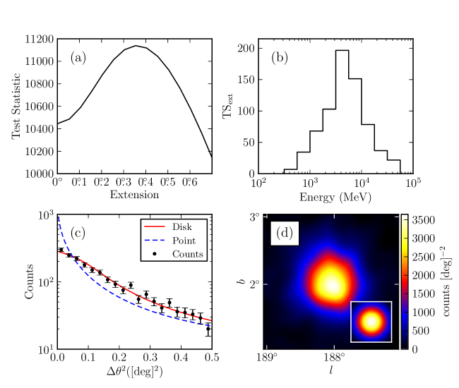
Figure 5.1: Counts maps and TS profiles for the SNR IC 443. (a) $\mathrm{TS}$ vs. extension of the source. (b) $\mathrm{TS}_{\mathrm{ext}}$ for individual energy bands. (c) observed radial profile of counts in comparison to the expected profiles for a spatially extended source (solid and colored red in the online version) and for a point-like source (dashed and colored blue in the online version). (d) smoothed counts map after subtraction of the diffuse emission compared to the smoothed LAT PSF (inset). Both were smoothed by a 0$.\!\!^{\circ}$1 2D Gaussian kernel. Plots (a), (c), and (d) use only photons with energies between 1 GeV and 100 GeV. Plots (c) and (d) include only photons which converted in the front part of the tracker and have an improved angular resolution (Atwood et al. 2009).

We estimate the error on the extension of a source by fixing the position of the source and varying the extension until the log of the likelihood has decreased by 1/2, corresponding to a $1\sigma$ error (Eadie et al. 1971). Figure 5.1 demonstrates this method by showing the change in the log of the likelihood when varying the modeled extension of the SNR IC 443. The localization error is calculated by fixing the extension and spectrum of the source to their best fit values and then fitting the log of the likelihood to a 2D Gaussian as a function of position. This localization error algorithm is further described in Nolan et al. (2012).

5.2.3 $\mathtt{gtlike}$ Analysis Validation

$\mathtt{pointlike}$ is important for analyses of LAT data that require many iterations such as source localization and extension fitting. On the other hand, because $\mathtt{gtlike}$ makes fewer approximations in calculating the likelihood we expect the spectral parameters found with $\mathtt{gtlike}$ to be slightly more accurate. Furthermore, because $\mathtt{gtlike}$ is the standard likelihood analysis package for LAT data, it has been more extensively validated for spectral analysis. For those reasons, in the following analysis we used $\mathtt{pointlike}$ to determine the position and extension of a source and subsequently derived the spectrum using $\mathtt{gtlike}$. Both $\mathtt{gtlike}$ and $\mathtt{pointlike}$ can be used to estimate the statistical significance of the extension of a source and we required that both methods agree for a source to be considered extended. There was good agreement between the two methods. Unless explicitly mentioned, all $\mathrm{TS}$, $\mathrm{TS}_{\mathrm{ext}}$, and spectral parameters were calculated using $\mathtt{gtlike}$ with the best-fit positions and extension found by $\mathtt{pointlike}$.

5.2.4 Comparing Source Sizes

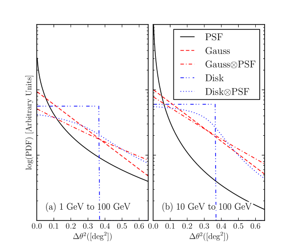
Figure 5.2: A comparison of a 2D Gaussian and uniform disk spatial model of extended sources before and after convolving with the PSF for two energy ranges. The solid black line is the PSF that would be observed for a power-law source of spectral index 2. The dashed line and the dash-dotted lines are the brightness profile of a Gaussian with ${\mathrm{r}_{68}}=0\mbox{$.\!\!^{\circ}$}5$ and the convolution of this profile with the LAT PSF respectively (colored red in the online version). The dash-dot-dotted and the dot-dotted lines are the brightness profile of a uniform disk with ${\mathrm{r}_{68}}=0\mbox{$.\!\!^{\circ}$}5$ and the convolution of this profile with the LAT PSF respectively (colored blue in the online version).

We considered two models for the surface brightness profile for extended sources: a 2D Gaussian model

$$I_{\text{Gaussian}}(x,y)=\tfrac{1}{2\pi\sigma^{2}}\exp\left(-(x^{2}+y^{2})/2\sigma^{2}\right)$$ (5.7)

or a uniform disk model

$$I_{\text{disk}}(x,y)=\begin{cases}\frac{1}{\pi\sigma^{2}}&x^{2}+y^{2}\leq\sigma^{2}\\ 0&x^{2}+y^{2}>\sigma^{2}.\end{cases}$$ (5.8)

Although these shapes are significantly different, Figure 5.2 shows that, after convolution with the LAT PSF, their PDFs are similar for a source that has a 0$.\!\!^{\circ}$5 radius typical of LAT-detected extended sources. To allow a valid comparison between the Gaussian and the uniform disk models, we define the source size as the radius containing 68% of the intensity (${\mathrm{r}_{68}}$). By direct integration, we find

$${\mathrm{r}_{68}}_{\text{,Gaussian}}= 1.51\sigma,$$ (5.9)

$${\mathrm{r}_{68}}_{\text{,disk}}= 0.82\sigma,$$ (5.10)

where $\sigma$ is defined in Equation 5.7 and Equation 5.8 respectively. For the example above, ${\mathrm{r}_{68}}=0\mbox{$.\!\!^{\circ}$}5$ so $\sigma_{\text{disk}}=0.61^{\circ}$ and $\sigma_{\text{Gaussian}}=0.33^{\circ}$.

For sources that are comparable in size to the PSF, the differences in the PDF for different spatial models are lost in the noise and the LAT is not sensitive to the detailed spatial structure of these sources. In Section 5.3.3, we perform a dedicated Monte Carlo simulation that shows there is little bias due to incorrectly modeling the spatial structure of an extended source. Therefore, in our search for extended sources we use only a radially-symmetric uniform disk spatial model. Unless otherwise noted, we quote the radius to the edge ($\sigma$) as the size of the source.

5.3 Validation of the TS Distribution

5.3.1 Point-like Source Simulations Over a Uniform Background

We tested the theoretical distribution for $\mathrm{TS}_{\mathrm{ext}}$ to evaluate the false detection probability for measuring source extension. To do so, we tested simulated point-like sources for extension. Mattox et al. (1996) discuss that the $\mathrm{TS}$ distribution for a likelihood-ratio test on the existence of a source at a given position is

$$P(\mathrm{TS})=\tfrac{1}{2}(\chi^{2}_{1}(\mathrm{TS})+\delta(\mathrm{TS})),$$ (5.11)

where $P(\mathrm{TS})$ is the probability density to get a particular value of TS, $\chi^{2}_{1}$ is the chi-squared distribution with one degree of freedom, and $\delta$ is the Dirac delta function. The particular form of Equation 5.11 is due to the null hypothesis (source flux $\Phi=0$) residing on the edge of parameter space and the model hypothesis adding a single degree of freedom (the source flux). It leads to the often quoted result $\sqrt{TS}=\sigma$, where $\sigma$ here refers to the significance of the detection. It is plausible to expect a similar distribution for the TS in the test for source extension since the same conditions apply (with the source flux $\Phi$ replaced by the source radius $r$ and $r<0$ being unphysical). To verify Equation 5.11, we evaluated the empirical distribution function of $\mathrm{TS}_{\mathrm{ext}}$ computed from simulated sources.

We simulated point-like sources with various spectral forms using the LAT on-orbit simulation tool $\mathtt{gtobssim}$ and fit the sources with $\mathtt{pointlike}$ using both point-like and extended source hypotheses. These point-like sources were simulated with a power-law spectral model with integrated fluxes above 100 MeV ranging from $3\times 10^{-9}$ to $1\times 10^{-5}$ $\text{ph}\;\text{cm}^{-2}\text{s}^{-1}$ and spectral indices ranging from 1.5 to 3. These values were picked to represent typical parameters of LAT-detected sources. The point-like sources were simulated on top of an isotropic background with a power-law spectral model with integrated flux above 100 MeV of $1.5\times 10^{-5}$ $\text{ph}\;\text{cm}^{-2}\text{s}^{-1}$ sr^-1 and spectral index 2.1. This was taken to be the same as the isotropic spectrum measured by EGRET (Sreekumar et al. 1998). This spectrum is comparable to the high-latitude background intensity seen by the LAT. The Monte Carlo simulation was performed over a one-year observation period using a representative spacecraft orbit and livetime. The reconstruction was performed using the P7_V6 Source class event selection and IRFs (Ackermann et al. 2012). For each significantly detected point-like source ($\mathrm{TS}\geq 25$), we used $\mathtt{pointlike}$ to fit the source as an extended source and calculate $\mathrm{TS}_{\mathrm{ext}}$. This entire procedure was performed twice, once fitting in the 1 GeV to 100 GeV energy range and once fitting in the 10 GeV to 100 GeV energy range.

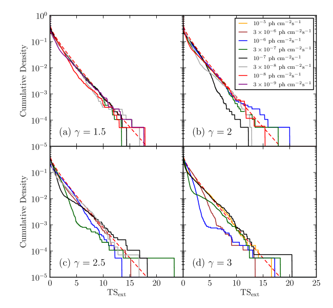
Figure 5.3: Cumulative distribution of the TS for the extension test when fitting simulated point-like sources in the 1 GeV to 100 GeV energy range. The four plots represent simulated sources of different spectral indices and the different lines (colored in the online version) represent point-like sources with different 100 MeV to 100 GeV integral fluxes. The dashed line (colored red) is the cumulative density function of Equation 5.11.

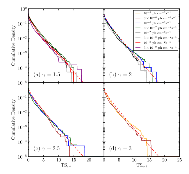
Figure 5.4: The same plot as Figure 5.3 but fitting in the 10 GeV to 100 GeV energy range.

Table 5.1: Monte Carlo Spectral Parameters

Spectral Index	Flux	$N_{1-100\text{GeV}}$	$\langle\mathrm{TS}\rangle_{1-100\text{GeV}}$	$N_{10-100\text{GeV}}$	$\langle\mathrm{TS}\rangle_{10-100\text{GeV}}$
	($\text{ph}\;\text{cm}^{-2}\text{s}^{-1}$)
Isotropic Background
1.5	$3\times 10^{-7}$	18938	22233	18938	8084
	$10^{-7}$	19079	5827	19079	2258
	$3\times 10^{-8}$	19303	1276	19303	541
	$10^{-8}$	19385	303	19381	142
	$3\times 10^{-9}$	18694	62	12442	43
2	$10^{-6}$	18760	22101	18760	3033
	$3\times 10^{-7}$	18775	4913	18775	730
	$10^{-7}$	18804	1170	18803	192
	$3\times 10^{-8}$	18836	224	15256	50
	$10^{-8}$	17060	50
2.5	$3\times 10^{-6}$	18597	19036	18597	786
	$10^{-6}$	18609	4738	18608	208
	$3\times 10^{-7}$	18613	954	15958	53
	$10^{-7}$	18658	203
	$3\times 10^{-8}$	14072	41
3	$10^{-5}$	18354	19466	18354	215
	$3\times 10^{-6}$	18381	4205	15973	54
	$10^{-6}$	18449	966
	$3\times 10^{-7}$	18517	174
	$10^{-7}$	13714	41
Galactic Diffuse and Isotropic Background
1.5	$2.3\times 10^{-8}$	90741	63
2	$1.2\times 10^{-7}$	92161	60
2.5	$4.5\times 10^{-7}$	86226	47
3	$2.0\times 10^{-6}$	94412	61

Note. — A list of the spectral models of the simulated point-like sources which were tested for extension. For each model, the number of statistically independent simulations and the average value of $\mathrm{TS}$ is also tabulated. The top rows are the simulations on top of an isotropic background and the bottom rows are the simulations on top of the Galactic diffuse and isotropic background.

For each set of spectral parameters, $\sim 20,000$ statistically independent simulations were performed. For lower-flux spectral models, many of the simulations left the source insignificant ($\mathrm{TS}<25$) and were discarded. Table 5.1 shows the different spectral models used in our study as well as the number of simulations and the average point-like source significance. The cumulative density of $\mathrm{TS}_{\mathrm{ext}}$ is plotted in Figure 5.3 and Figure 5.4 and compared to the $\chi^{2}_{1}/2$ distribution of Equation 5.11.

Our study shows broad agreement between simulations and Equation 5.11. To the extent that there is a discrepancy, the simulations tended to produce smaller than expected values of $\mathrm{TS}_{\mathrm{ext}}$ which would make the formal significance conservative. Considering the distribution in Figure 5.3 and Figure 5.4, the choice of a threshold $\mathrm{TS}_{\mathrm{ext}}$ set to 16 (corresponding to a formal $4\sigma$ significance) is reasonable.

5.3.2 Point-like Source Simulations Over a Structured Background

We performed a second set of simulations to show that the theoretical distribution for $\mathrm{TS}_{\mathrm{ext}}$ is still preserved when the point-like sources are present over a highly-structured diffuse background. Our simulation setup was the same as above except that the sources were simulated on top of and analyzed assuming the presence of the standard Galactic diffuse and isotropic background models used in 2FGL. In our simulations, we selected our sources to have random positions on the sky such that they were within 5^∘ of the Galactic plane. This probes the brightest and most strongly contrasting areas of the Galactic background.

To limit the number of tests, we selected only one flux level for each of the four spectral indices and we performed this test only in the 1 GeV to 100 GeV energy range. As described below, the fluxes were selected so that $\mathrm{TS}\sim 50$. We do not expect to be able to spatially resolve sources at lower fluxes than these, and the results for much brighter sources are less likely to be affected by the structured background.

Because the Galactic diffuse emission is highly structured with strong gradients, the point-source sensitivity can vary significantly across the Galactic plane. To account for this, we scaled the flux (for a given spectral index) so that the source always has approximately the same signal-to-noise ratio:

$$F(\vec{x})=F(\text{GC})\times\left(\frac{B(\vec{x})}{B(\text{GC})}\right)^{1/2}.$$ (5.12)

Here, $\vec{x}$ is the position of the simulated source, $F$ is the integral flux of the source from 100 MeV to 100 GeV, $F(\text{GC})$ is the same quantity if the source was at the Galactic center, $B$ is the integral of the Galactic diffuse and isotropic emission from 1 GeV to 100 GeV at the position of the source, and $B(\text{GC})$ is the same quantity if the source was at the Galactic center. For the four spectral models, Table 5.1 lists $F(\text{GC})$ and the average value of $\mathrm{TS}$.

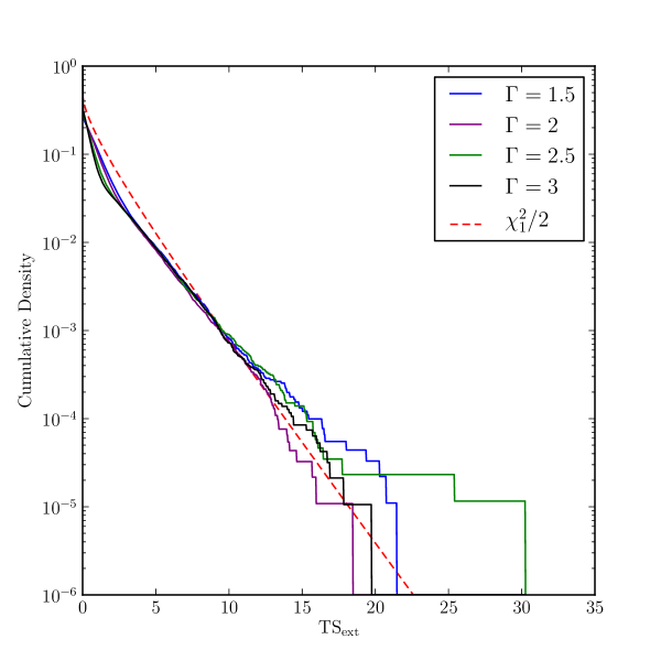
Figure 5.5: Cumulative distribution of $\mathrm{TS}_{\mathrm{ext}}$ for sources simulated on top of the Galactic diffuse and isotropic background.

For each spectrum, we performed $\sim 90,000$ simulations. Figure 5.5 shows the cumulative density of $\mathrm{TS}_{\mathrm{ext}}$ for each spectrum. For small values of $\mathrm{TS}_{\mathrm{ext}}$, there is good agreement between the simulations and theory. For the highest values of $\mathrm{TS}_{\mathrm{ext}}$, there is possibly a small discrepancy, but the discrepancy is not statistically significant. Therefore, we are confident we can use $\mathrm{TS}_{\mathrm{ext}}$ as a robust measure of statistical significance when testing LAT-detected sources for extension.

5.3.3 Extended Source Simulations Over a Structured Background

We also performed a Monte Carlo study to show that incorrectly modeling the spatial extension of an extended source does not substantially bias the spectral fit of the source, although it does alter the value of the $\mathrm{TS}$. To assess this, we simulated the spatially extended ring-type SNR W44. We selected W44 because it is the most significant extended source detected by the LAT that has a non-radially symmetric photon distribution (Abdo et al. 2010a).

W44 was simulated with a power-law spectral model with an integral flux of $7.12\times 10^{-8}$ $\text{ph}\;\text{cm}^{-2}\text{s}^{-1}$ in the energy range from 1 GeV to 100 GeV and a spectral index of 2.66 (see Section 6.1).

W44 was simulated with the elliptical ring spatial model described in Abdo et al. (2010a). For reference, the ellipse has a semi-major axis of 0$.\!\!^{\circ}$3, a semi-minor axis of 0$.\!\!^{\circ}$19, a position angle of $147^{\circ}$ measured East of celestial North, and the ring’s inner radius is 75% of the outer radius.

We used a simulation setup similar to that described in Section 5.3.2, but the simulations were over the 2-year interval of the 2FGL catalog. In the simulations, we did not include the finite energy resolution of the LAT to isolate any effects due to changing the assumed spatial model. The fitting code we use also ignores this energy dispersion and the potential bias introduced by this will be discussed in an upcoming paper by the LAT collaboration (Ackermann et al. 2012). In total, we performed 985 independent simulations.

The simulated sources were fit using a point-like spatial model, a radially-symmetric Gaussian spatial model, a uniform disk spatial model, an elliptical disk spatial model, and finally with an elliptical ring spatial model. We obtained the best fit spatial parameters using $\mathtt{pointlike}$ and, with these parameters, obtained the best fit spectral parameters using $\mathtt{gtlike}$.

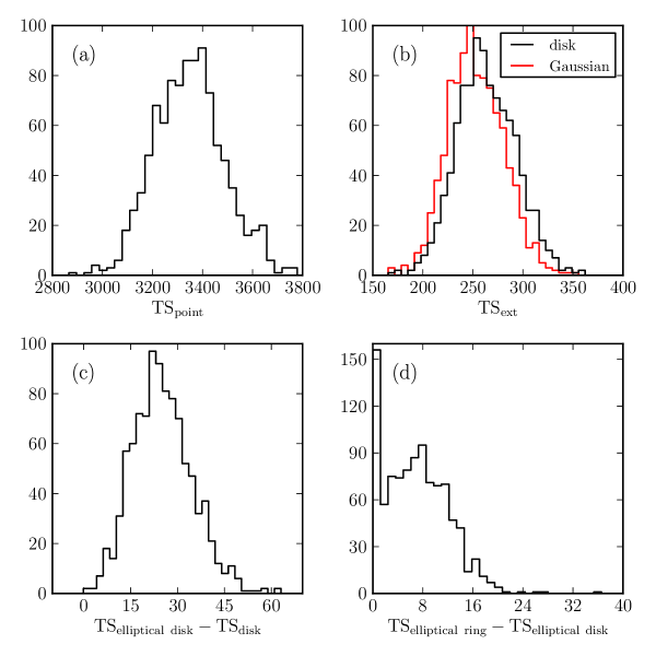
Figure 5.6: The distribution of $\mathrm{TS}$ values when fitting 985 statistically independent simulations of W44. (a) is the distribution of $\mathrm{TS}$ values when fitting W44 as a point-like source and (b) is the distribution of $\mathrm{TS}_{\mathrm{ext}}$ when fitting the source with a uniform disk or a radially-symmetric Gaussian spatial model. (c) is the distribution of the change in TS when fitting the source with an elliptical disk spatial model compared to fitting it with a radially-symmetric disk spatial model and (d) when fitting the source with an elliptical ring spatial model compared to an elliptical disk spatial model.

Figure 5.6a shows that the significance of W44 in the simulations is very large ($\mathrm{TS}\sim 3500$) for a model with a point-like source hypothesis. Figure 5.6b shows that the significance of the spatial extension is also large ($\mathrm{TS}_{\mathrm{ext}}\sim 250$). On average $\mathrm{TS}_{\mathrm{ext}}$ is somewhat larger when fitting the sources with more accurate spatial models. This shows that assuming an incorrect spatial model will cause the source’s significance to be underestimated. Figure 5.6c shows that the sources were fit better when assuming an elliptical disk spatial model compared to a uniform disk spatial model ($\mathrm{TS}_{\text{elliptical\ disk}}-\mathrm{TS}_{\text{disk}}\sim 30$). Finally, Figure 5.6d shows that the sources were fit somewhat better assuming an elliptical ring spatial model compared to an elliptical disk spatial model ($\mathrm{TS}_{\text{elliptical\ ring}}-\mathrm{TS}_{\text{elliptical\ disk}}\sim 9$). This shows that the LAT has some additional power to resolve substructure in bright extended sources.

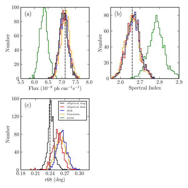
Figure 5.7: The distribution of fit parameters for the Monte Carlo simulations of W44. The plots show the distribution of best fit (a) flux (b) spectral index and (c) 68% containment radius. The dashed vertical lines represent the simulated values of the parameters.

Figure 5.7a and Figure 5.7b clearly show that no significant bias is introduced by modeling the source as extended but with an inaccurate spatial model, while a point-like source modeling results in a $\sim 10\%$ and $\sim 0.125$ bias in the fit flux and index, respectively. Furthermore, Figure 5.7c shows that the $\mathrm{r}_{68}$ estimate of the extension size is very mildly biased ($\sim 10\%$) toward higher values when inaccurate spatial models are used, and thus represents a reasonable measurement of the true 68% containment radius for the source. For the elliptical spatial models, $\mathrm{r}_{68}$ is computed by numeric integration.

5.4 Extended Source Detection Threshold

We calculated the LAT flux threshold to detect spatial extent. We define the detection threshold as the flux at which the value of $\mathrm{TS}_{\mathrm{ext}}$ averaged over many statistical realizations is $\langle\mathrm{TS}_{\mathrm{ext}}\rangle=16$ (corresponding to a formal $4\sigma$ significance) for a source of a given extension.

We used a simulation setup similar to that described in Section 5.3.1, but instead of point-like sources we simulated extended sources with radially-symmetric uniform disk spatial models. Additionally, we simulated our sources over the two-year time range included in the 2FGL catalog. For each extension and spectral index, we selected a flux range which bracketed $\mathrm{TS}_{\mathrm{ext}}=16$ and performed an extension test for $>100$ independent realizations of ten fluxes in the range. We calculated $\langle\mathrm{TS}_{\mathrm{ext}}\rangle=16$ by fitting a line to the flux and $\mathrm{TS}_{\mathrm{ext}}$ values in the narrow range.

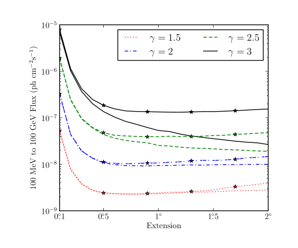
Figure 5.8: The detection threshold to resolve an extended source with a uniform disk model for a two-year exposure. All sources have an assumed power-law spectrum and the different line styles (colors in the electronic version) correspond to different simulated spectral indices. The lines with no markers correspond to the detection threshold using photons with energies between 100 MeV and 100 GeV, while the lines with star-shaped markers correspond to the threshold using photons with energies between 1 GeV and 100 GeV.

Figure 5.8 shows the threshold for sources of four spectral indices from 1.5 to 3 and extensions varying from $\sigma=0\mbox{$.\!\!^{\circ}$}1$ to $2\mbox{$.\!\!^{\circ}$}0$. The threshold is high for small extensions when the source is small compared to the size of the PSF. It drops quickly with increasing source size and reaches a minimum around 0$.\!\!^{\circ}$5. The threshold increases for large extended sources because the source becomes increasingly diluted by the background. Figure 5.8 shows the threshold using photons with energies between 100 MeV and 100 GeV and also using only photons with energies between 1 GeV and 100 GeV. Except for very large or very soft sources, the threshold is not substantially improved by including photons with energies between 100 MeV and 1 GeV. This is also demonstrated in Figure 5.1 which shows $\mathrm{TS}_{\mathrm{ext}}$ for the SNR IC 443 computed independently in twelve energy bins between 100 MeV and 100 GeV. For IC 443, which has a spectral index $\sim 2.4$ and an extension $\sim 0\mbox{$.\!\!^{\circ}$}35$, almost the entire increase in likelihood from optimizing the source extent in the model comes from energies above 1 GeV. Furthermore, other systematic errors become increasingly large at low energy. For our extension search (Section 6.3), we therefore used only photons with energies above 1 GeV.

Table 5.2: Extension Detection Threshold

$\gamma$	BG	$0.1$	$0.2$	$0.3$	$0.4$	$0.5$	$0.6$	$0.7$	$0.8$	$0.9$	$1.0$	$1.1$	$1.2$	$1.3$	$1.4$	$1.5$	$1.6$	$1.7$	$1.8$	$1.9$	$2.0$
E$>$1 GeV
1.5	$1\times$	148.1	23.3	11.3	8.0	7.2	6.9	6.7	6.8	7.1	7.4	7.6	7.9	8.1	8.5	9.2	9.9	9.1	9.2	9.0	10.3
	$10\times$	148.4	29.0	18.7	15.2	15.4	15.0	16.1	16.0	16.8	17.7	18.2	19.3	20.9	22.5	23.8	24.8	21.3	22.8	23.4	23.7
	$100\times$	186.8	55.0	43.4	40.7	41.0	41.8	40.9	40.9	42.7	43.6	38.4	39.9	40.6	38.4	36.9	36.3	37.1	38.8	37.2	37.6
2	$1\times$	328.4	43.4	18.9	13.4	11.2	10.4	10.2	10.2	10.2	10.4	10.7	10.9	11.2	11.5	12.4	12.6	13.0	13.4	14.0	14.4
	$10\times$	341.0	55.9	32.3	27.6	26.5	25.4	25.6	25.9	27.4	26.8	27.8	28.7	29.8	30.1	31.0	31.5	31.7	34.0	34.3	35.9
	$100\times$	420.5	128.3	90.2	77.3	73.3	70.8	67.5	64.3	64.2	64.1	62.8	63.6	61.7	61.9	58.4	59.0	61.4	63.3	60.1	58.1
2.5	$1\times$	627.1	75.6	29.8	19.3	15.5	13.5	12.8	12.6	12.5	12.5	12.6	12.9	12.9	13.1	13.5	13.7	14.3	14.8	15.2	15.8
	$10\times$	638.9	99.1	52.1	39.1	34.6	33.0	32.5	32.5	32.8	33.2	34.1	34.3	34.5	35.1	36.6	36.9	35.5	36.0	36.5	37.3
	$100\times$	795.0	262.1	140.9	104.3	90.4	81.2	77.2	75.1	69.7	70.9	66.5	65.6	64.9	64.0	58.9	58.1	60.2	58.4	57.5	55.8
3	$1\times$	841.5	110.6	43.2	25.5	18.7	16.1	14.4	13.6	13.3	13.2	13.1	13.1	13.4	13.6	13.5	13.8	14.2	14.4	14.8	15.4
	$10\times$	921.6	151.3	69.1	47.8	40.7	37.1	35.5	34.5	35.1	35.5	35.3	35.3	35.4	35.5	36.8	37.6	35.3	35.4	36.3	36.6
	$100\times$	1124.1	282.9	181.1	119.8	100.7	91.1	84.3	77.9	73.3	71.8	67.6	66.4	65.5	63.9	59.0	58.6	58.8	57.5	55.4	54.4
E$>$10 GeV
1.5	$1\times$	44.6	8.0	4.3	3.2	2.7	2.6	2.5	2.5	2.4	2.5	2.5	2.6	2.7	2.8	2.9	2.9	3.1	3.2	3.3	3.4
	$10\times$	45.2	9.2	5.8	5.0	4.9	4.9	5.0	5.2	5.3	5.7	5.9	6.3	6.6	6.5	6.8	7.6	7.8	8.2	8.5	8.7
	$100\times$	47.3	13.4	11.6	10.6	10.8	10.8	12.0	12.7	13.2	13.7	15.3	16.1	17.2	18.2	18.9	19.5	20.4	21.0	21.7	22.9
2	$1\times$	49.7	8.4	4.4	3.3	2.8	2.6	2.6	2.6	2.6	2.6	2.7	2.7	2.8	2.9	3.0	3.2	3.2	3.4	3.5	3.5
	$10\times$	48.6	9.5	6.0	5.2	5.0	5.2	5.2	5.3	5.4	5.8	6.4	6.6	7.0	7.1	7.5	8.0	8.3	8.6	9.0	9.2
	$100\times$	51.8	14.7	11.8	11.5	11.5	11.9	13.2	14.0	14.3	15.3	16.2	16.9	18.4	19.2	19.8	21.0	22.0	22.8	23.2	24.3
2.5	$1\times$	53.1	9.1	4.5	3.3	2.8	2.7	2.6	2.5	2.5	2.6	2.7	2.7	2.8	2.8	2.9	3.1	3.2	3.3	3.5	3.6
	$10\times$	53.7	10.5	6.3	5.4	5.1	5.1	5.3	5.4	5.7	6.0	6.3	6.6	6.8	6.9	7.5	8.1	8.3	8.6	8.9	9.2
	$100\times$	57.0	15.6	12.7	11.9	11.8	12.2	13.1	14.3	14.6	15.2	16.3	17.0	18.8	19.2	19.9	21.0	21.9	22.3	23.3	23.7
3	$1\times$	55.5	9.4	4.8	3.4	2.9	2.7	2.6	2.5	2.5	2.5	2.6	2.7	2.7	2.8	2.9	3.0	3.1	3.2	3.4	3.4
	$10\times$	56.0	10.5	6.2	5.3	5.1	5.1	5.1	5.3	5.5	5.7	5.9	6.4	6.4	6.6	7.0	7.8	8.0	8.3	8.6	8.9
	$100\times$	60.3	16.2	12.7	11.7	11.8	12.2	12.6	13.8	14.2	14.6	15.8	16.5	17.6	18.5	19.4	19.8	20.7	21.0	21.8	22.5

Note. — The detection threshold to resolve spatially extended sources with a uniform disk spatial model for a two-year exposure The threshold is calculated for sources of varying energy ranges, spectral indices, and background levels. The sensitivity was calculated against a Sreekumar-like isotropic background and the second column is the factor that the simulated background was scaled by. The remaining columns are varying sizes of the source. The table quotes integral fluxes in the analyzed energy range (1 GeV to 100 GeV or 10 GeV to 100 GeV) in units of $10^{-10}$ $\text{ph}\;\text{cm}^{-2}\text{s}^{-1}$.

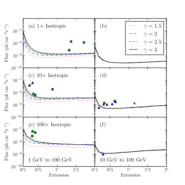
Figure 5.9: The LAT detection threshold for four spectral indices and three backgrounds ($1\times$, $10\times$, and $100\times$ the Sreekumar-like isotropic background) for a two-year exposure. The left-hand plots are the detection threshold when using photons with energies between 1 GeV and 100 GeV and the right-hand plots are the detection threshold when using photons with energies between 10 GeV and 100 GeV. The flux is integrated only in the selected energy range. Overlaid on this plot are the LAT-detected extended sources placed by the magnitude of the nearby Galactic diffuse emission and the energy range they were analyzed with. The star-shaped markers (colored red in the electronic version) are sources with a spectral index closer to 1.5, the triangular markers (colored blue) an index closer to 2, and the circular markers (colored green) an index closer to 2.5. The triangular marker in plot (d) below the sensitivity line is MSH 15$-$52.

Figure 5.9 shows the flux threshold as a function of source extension for different background levels ($1\times$, $10\times$, and $100\times$ the nominal background), different spectral indices, and two different energy ranges (1 GeV to 100 GeV and 10 GeV to 100 GeV). The detection threshold is higher for sources in regions of higher background. When studying sources only at energies above 1 GeV, the LAT detection threshold (defined as the 1 GeV to 100 GeV flux at which $\langle\mathrm{TS}_{\mathrm{ext}}\rangle=16$) depends less strongly on the spectral index of the source. The index dependence of the detection threshold is even weaker when considering only photons with energies above 10 GeV because the PSF changes little from 10 GeV to 100 GeV. Overlaid on Figure 5.9 are the LAT-detected extended sources that will be discussed in Section 6.1 and Section 6.4. The extension thresholds are tabulated in Table 5.2.

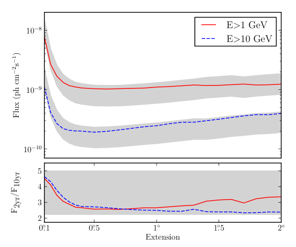
Figure 5.10: The projected detection threshold of the LAT to extension after 10 years for a power-law source of spectral index 2 against 10 times the isotropic background in the energy range from 1 GeV to 100 GeV (solid line colored red in the electronic version) and 10 GeV to 100 GeV (dashed line colored blue). The shaded gray regions represent the detection threshold assuming the sensitivity improves from 2 to 10 years by the square root of the exposure (top edge) and linearly with exposure (bottom edge). The lower plot shows the factor increase in sensitivity. For small extended sources, the detection threshold of the LAT to the extension of a source will improve by a factor larger than the square root of the exposure.

Finally, Figure 5.10 shows the projected detection threshold of the LAT to extension with a 10 year exposure against 10 times the isotropic background measured by EGRET. This background is representative of the background near the Galactic plane. For small extended sources, the threshold improves by a factor larger than the square root of the relative exposures because the LAT is signal-limited at high energies where the present analysis is most sensitive. For large extended sources, the relevant background is over a larger spatial range and so the improvement is closer to a factor corresponding to the square root of the relative exposures that is caused by Poisson fluctuations in the background.

5.5 Testing Against Source Confusion

It is impossible to discriminate using only LAT data between a spatially extended source and multiple point-like sources separated by angular distances comparable to or smaller than the size of the LAT PSF. To assess the plausibility of source confusion for sources with $\mathrm{TS}_{\mathrm{ext}}\geq 16$, we developed an algorithm to test if a region contains two point-like sources. The algorithm works by simultaneously fitting in $\mathtt{pointlike}$ the positions and spectra of the two point-like sources. To help with convergence, it begins by dividing the source into two spatially coincident point-like sources and then fitting the sum and difference of the positions of the two sources without any limitations on the fit parameters.

After simultaneously fitting the two positions and two spectra, we define $\mathrm{TS}_{\mathrm{2pts}}$ as twice the increase in the log of the likelihood fitting the region with two point-like sources compared to fitting the region with one point-like source:

$$\mathrm{TS}_{\mathrm{2pts}}=2\log(\mathcal{L}_{\text{2pts}}/\mathcal{L}_{\text{ps}}).$$ (5.13)

For the following analysis of LAT data, $\mathrm{TS}_{\mathrm{2pts}}$ was computed by fitting the spectra of the two point-like sources in $\mathtt{gtlike}$ using the best fit positions of the sources found by $\mathtt{pointlike}$.

$\mathrm{TS}_{\mathrm{2pts}}$ cannot be quantitatively compared to $\mathrm{TS}_{\mathrm{ext}}$ using a simple likelihood-ratio test to evaluate which model is significantly better because the models are not nested (Protassov et al. 2002). Even though the comparison of $\mathrm{TS}_{\mathrm{ext}}$ with $\mathrm{TS}_{\mathrm{2pts}}$ is not a calibrated test, $\mathrm{TS}_{\mathrm{ext}}>\mathrm{TS}_{\mathrm{2pts}}$ indicates that the likelihood for the extended source hypothesis is higher than for two point-like sources and we only consider a source to be extended if $\mathrm{TS}_{\mathrm{ext}}>\mathrm{TS}_{\mathrm{2pts}}$.

We considered using the Bayesian information criterion (BIC, Schwarz 1978) as an alternative Bayesian formulation for this test, but it is difficult to apply to LAT data because it contains a term including the number of data points. For studying $\gamma$-ray sources in LAT data, we analyze relatively large regions of the sky to better define the contributions from diffuse backgrounds and nearby point sources. This is important for accurately evaluating source locations and fluxes but the fraction of data directly relevant to the evaluation of the parameters for the source of interest is relatively small.

As an alternative, we considered the Akaike information criterion test (AIC, Akaike 1974). The AIC is defined as $\text{AIC}=2k-2\log\mathcal{L}$, where $k$ is the number of parameters in the model. In this formulation, the best hypothesis is considered to be the one that minimizes the AIC. The first term penalizes models with additional parameters.

The two point-like sources hypothesis has three more parameters than the single extended source hypothesis (two more spatial parameters and two more spectral parameters compared to one extension parameter), so the comparison $\text{AIC}_{\text{ext}}<\text{AIC}_{\text{2pts}}$ is formally equivalent to $\mathrm{TS}_{\mathrm{ext}}+6>\mathrm{TS}_{\mathrm{2pts}}$. Our criterion for accepting extension ($\mathrm{TS}_{\mathrm{ext}}>\mathrm{TS}_{\mathrm{2pts}}$) is thus equivalent to requesting that the AIC-based empirical support for the two point-like sources model be “considerably less” than for the extended source model, following the classification by Burnham & Anderson (2002).

We assessed the power of the $\mathrm{TS}_{\mathrm{ext}}>\mathrm{TS}_{\mathrm{2pts}}$ test with a Monte Carlo study. We simulated one spatially extended source and fit it as both an extended source and as two point-like sources using $\mathtt{pointlike}$. We then simulated two point-like sources and fit them with the same two hypotheses. By comparing the distribution of $\mathrm{TS}_{\mathrm{2pts}}$ and $\mathrm{TS}_{\mathrm{ext}}$ computed by $\mathtt{pointlike}$ for the two cases, we evaluated how effective the $\mathrm{TS}_{\mathrm{ext}}>\mathrm{TS}_{\mathrm{2pts}}$ test is at rejecting cases of source confusion as well as how likely it is to incorrectly reject that an extended source is spatially extended. All sources were simulated using the same time range as in Section 5.4 against a background 10 times the isotropic background measured by EGRET, representative of the background near the Galactic plane.

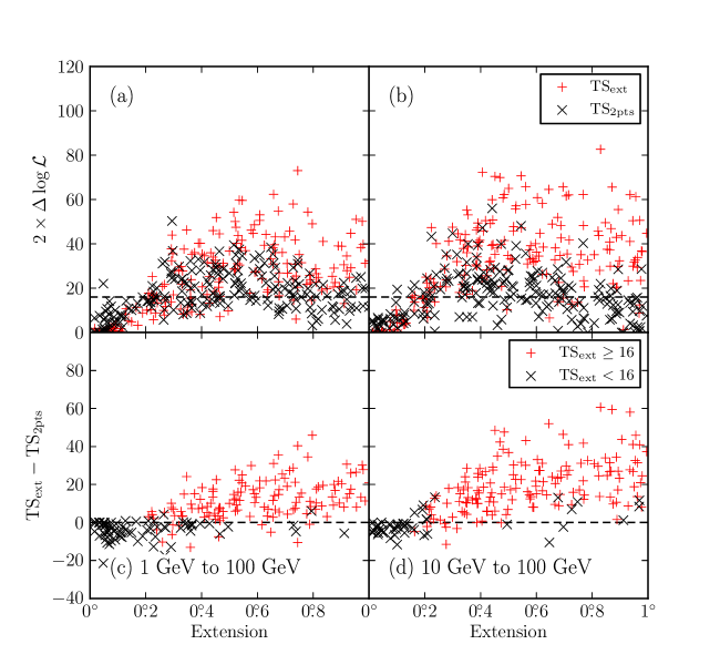
Figure 5.11: (a) and (b) are the distribution of $\mathrm{TS}_{\mathrm{ext}}$ and of $\mathrm{TS}_{\mathrm{2pts}}$ when fitting simulated spatially extended sources of varying sizes as both an extended source and as two point-like sources. (c) and (d) are the distribution of $\mathrm{TS}_{\mathrm{ext}}-\mathrm{TS}_{\mathrm{2pts}}$ for the same simulated sources. (a) and (c) represent sources fit in the 1 GeV to 100 GeV energy range and (b) and (d) represent sources fit in the 10 GeV to 100 GeV energy range. In (c) and (d), the plus-shaped markers (colored red in the electronic version) are fits where $\mathrm{TS}_{\mathrm{ext}}\geq 16$.

We did this study first in the energy range from 1 GeV to 100 GeV by simulating extended sources of flux $4\times 10^{-9}$ $\text{ph}\;\text{cm}^{-2}\text{s}^{-1}$ integrated from 1 GeV to 100 GeV and a power-law spectral model with spectral index 2. This spectrum was picked to be representative of the new extended sources that were discovered in the following analysis when looking in the 1 GeV to 100 GeV energy range (see Section 6.4). We simulated these sources using uniform disk spatial models with extensions varying up to $1^{\circ}$. Figure 5.11a shows the distribution of $\mathrm{TS}_{\mathrm{ext}}$ and $\mathrm{TS}_{\mathrm{2pts}}$ and Figure 5.11c shows the distribution of $\mathrm{TS}_{\mathrm{ext}}-\mathrm{TS}_{\mathrm{2pts}}$ as a function of the simulated extension of the source for 200 statistically independent simulations.

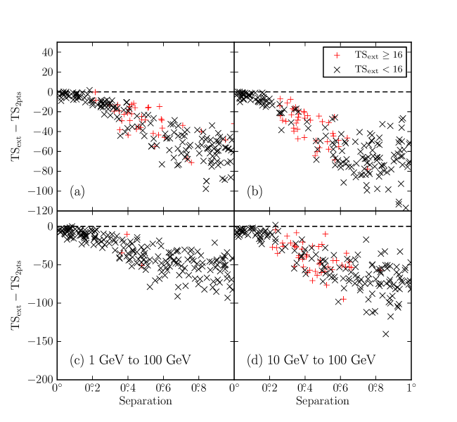
Figure 5.12: The distribution of $\mathrm{TS}_{\mathrm{ext}}-\mathrm{TS}_{\mathrm{2pts}}$ when fitting two simulated point-like sources of varying separations as both an extended source and as two point-like sources. (a), and (b) represent simulations of two point-like sources with the same spectral index and (c) and (d) represent simulations of two point-like sources with different spectral indices. (a) and (c) fit the simulated sources in the 1 GeV to 100 GeV energy range and (b) and (d) fit in the 10 GeV to 100 GeV energy range. The plus-shaped markers (colored red in the electronic version) are fits where $\mathrm{TS}_{\mathrm{ext}}\geq 16$.

Figure 5.12a shows the same plot but when fitting two simulated point-like sources each with half of the flux of the spatially extended source and with the same spectral index as the extended source. Finally, Figure 5.12c shows the same plot with each point-like source having the same flux but different spectral indices. One point-like source had a spectral index of 1.5 and the other an index of 2.5. These indices are representative of the range of indices of LAT-detected sources.

The same four plots are shown in Figure 5.11b, Figure 5.11d, Figure 5.12b, and Figure 5.12d but this time when analyzing a source of flux $10^{-9}$ $\text{ph}\;\text{cm}^{-2}\text{s}^{-1}$ (integrated from 10 GeV to 100 GeV) only in the 10 GeV to 100 GeV energy range. This flux is typical of the new extended sources discovered using only photons with energies between 10 GeV and 100 GeV (see Section 6.4).

Several interesting conclusions can be made from this study. As one would expect, $\mathrm{TS}_{\mathrm{ext}}-\mathrm{TS}_{\mathrm{2pts}}$ is mostly positive when fitting the simulated extended sources. In the 1 GeV to 100 GeV analysis, only 11 of the 200 simulated extended sources had $\mathrm{TS}_{\mathrm{ext}}>16$ but were incorrectly rejected due to $\mathrm{TS}_{\mathrm{2pts}}$ being greater than $\mathrm{TS}_{\mathrm{ext}}$. In the 10 GeV to 100 GeV analysis, only 7 of the 200 sources were incorrectly rejected. From this, we conclude that this test is unlikely to incorrectly reject truly spatially extended sources.

On the other hand, it is often the case that $\mathrm{TS}_{\mathrm{ext}}>16$ when testing the two simulated point-like sources for extension. This is especially the case when the two sources had the same spectral index. Forty out of 200 sources in the 1 GeV to 100 GeV energy range and 43 out of 200 sources in the 10 GeV to 100 GeV energy range had $\mathrm{TS}_{\mathrm{ext}}>16$. But in these cases, we always found the single extended source fit to be worse than the two point-like source fit. From this, we conclude that the $\mathrm{TS}_{\mathrm{ext}}>\mathrm{TS}_{\mathrm{2pts}}$ test is powerful at discarding cases in which the true emission comes from two point-like sources.

The other interesting feature in Figure 5.11a and Figure 5.11b is that for simulated extended sources with typical sizes ($\sigma\sim 0\mbox{$.\!\!^{\circ}$}5$), one can often obtain almost as large an increase in likelihood fitting the source as two point-like sources ($\mathrm{TS}_{\mathrm{2pts}}\sim\mathrm{TS}_{\mathrm{ext}}$). This is because although the two point-like sources represent an incorrect spatial model, the second source has four additional degrees of freedom (two spatial and two spectral parameters) and can therefore easily model much of the extended source and statistical fluctuations in the data. This effect is most pronounced when using photons with energies between 1 GeV and 100 GeV where the PSF is broader.

From this Monte Carlo study, we can see the limits of an analysis with LAT data of spatially extended sources. Section 5.3.1 showed that we have a statistical test that finds when a LAT source is not well described by the PSF. But this test does not uniquely prove that the emission originates from spatially extended emission instead of from multiple unresolved sources. Demanding that $\mathrm{TS}_{\mathrm{ext}}>\mathrm{TS}_{\mathrm{2pts}}$ is a powerful second test to avoid cases of simple confusion of two point-like sources. But it could always be the case that an extended source is actually the superposition of multiple point-like or extended sources that could be resolved with deeper observations of the region. There is nothing about this conclusion unique to analyzing LAT data, but the broad PSF of the LAT and the density of sources expected to be GeV emitters in the Galactic plane makes this issue more significant for analyses of LAT data. When possible, multiwavelength information should be used to help select the best model of the sky.

5.6 Test of 2LAC Sources

For all following analyses of LAT data, we used the same two-year dataset that was used in the 2FGL catalog spanning from 2008 August 4 to 2010 August 1. We applied the same acceptance cuts and we used the same P7_V6 Source class event selection and IRFs (Ackermann et al. 2012). When analyzing sources in $\mathtt{pointlike}$, we used a circular $10^{\circ}$ region of interest (ROI) centered on our source and eight energy bins per logarithmic decade in energy. When refitting the region in $\mathtt{gtlike}$ using the best fit spatial and spectral models from $\mathtt{pointlike}$, we used the ‘binned likelihood’ mode of $\mathtt{gtlike}$ on a $14^{\circ}\times 14^{\circ}$ ROI with a pixel size of 0$.\!\!^{\circ}$03.

Unless explicitly mentioned, we used the same background model as 2FGL to represent the Galactic diffuse, isotropic, and Earth limb emission. To compensate for possible residuals in the diffuse emission model, the Galactic emission was scaled by a power-law and the normalization of the isotropic component was left free. Unless explicitly mentioned, we used all 2FGL sources within $15^{\circ}$ of our source as our list of background sources and we refit the spectral parameters of all sources within $2^{\circ}$ of the source.

To validate our method, we tested LAT sources associated with AGN for extension. GeV emission from AGN is believed to originate from collimated jets. Therefore AGN are not expected to be spatially resolvable by the LAT and provide a good calibration source to demonstrate that our extension detection method does not misidentify point-like sources as being extended. We note that megaparsec-scale $\gamma$-ray halos around AGNs have been hypothesized to be resolvable by the LAT (Aharonian et al. 1994). However, no such halo has been discovered in the LAT data so far (Neronov et al. 2011).

Following 2FGL, the LAT Collaboration published the Second LAT AGN Catalog (2LAC), a list of high latitude ($|b|>10^{\circ}$) sources that had a high probability association with AGN (Ackermann et al. 2011b). 2LAC associated 1016 2FGL sources with AGN. To avoid systematic problems with AGN classification, we selected only the 885 AGN which made it into the clean AGN sub-sample defined in the 2LAC paper. An AGN association is considered clean only if it has a high probability of association $P\geq 80\%$, if it is the only AGN associated with the 2FGL source, and if no analysis flags have been set for the source in the 2FGL catalog. These last two conditions are important for our analysis. Source confusion may look like a spatially extended source and flagged 2FGL sources may correlate with unmodeled structure in the diffuse emission.

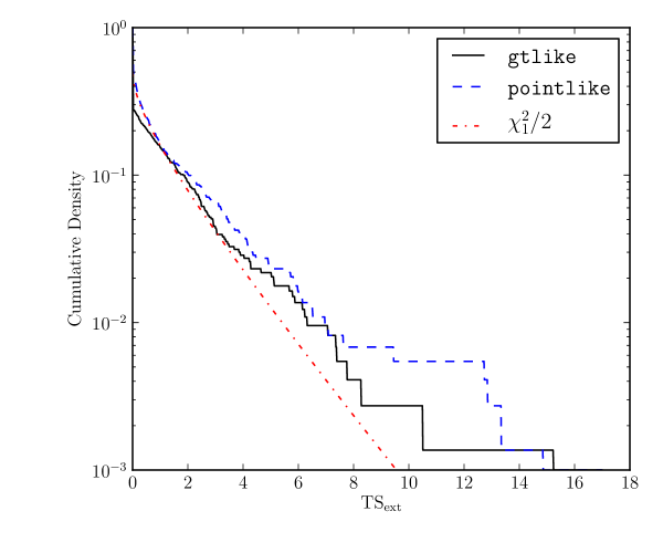
Figure 5.13: The cumulative density of $\mathrm{TS}_{\mathrm{ext}}$ for the 733 clean AGN in 2LAC that were significant above 1 GeV calculated with $\mathtt{pointlike}$ (dashed line colored blue in the electronic version) and with $\mathtt{gtlike}$ (solid line colored black). AGN are too far and too small to be resolved by the LAT. Therefore, the cumulative density of $\mathrm{TS}_{\mathrm{ext}}$ is expected to follow a $\chi^{2}_{1}/2$ distribution (Equation 5.11, the dash-dotted line colored red).

Of the 885 clean AGN, we selected the 733 of these 2FGL sources which were significantly detected above 1 GeV and fit each of them for extension. The cumulative density of $\mathrm{TS}_{\mathrm{ext}}$ for these AGN is compared to the $\chi^{2}_{1}/2$ distribution of Equation 5.11 in Figure 5.13. The $\mathrm{TS}_{\mathrm{ext}}$ distribution for the AGN shows reasonable agreement with the theoretical distribution and no AGN was found to be significantly extended ($\mathrm{TS}_{\mathrm{ext}}>16$). The observed discrepancy from the theoretical distribution is likely due to small systematics in our model of the LAT PSF and the Galactic diffuse emission (see Section 6.2). The discrepancy could also in a few cases be due to confusion with a nearby undetected source. We note that the Monte Carlo study of Section 5.3.1 effectively used perfect IRFs and a perfect model of the sky. The overall agreement with the expected distribution demonstrates that we can use $\mathrm{TS}_{\mathrm{ext}}$ as a measure of the statistical significance of the detection of the extension of a source.

We note that the LAT PSF used in this study was determined empirically by fitting the distributions of gamma rays around bright AGN (see Section 6.2). Finding that the AGN we test are not extended is not surprising. This validation analysis is not suitable to reject any hypotheses about the existence of megaparsec-scale halos around AGN.

Chapter 6 Search for Spatially-extended LAT Sources

This chapter is based the second part of the paper “Search for Spatially Extended Fermi-LAT Sources Using Two Years of Data” (Lande et al. 2012).

In Chapter 5, we developed a new method to study spatially-extended sources. In this chapter, we apply this method to search for new spatially-extended sources. In Section 6.1, we systematically reanalyze the twelve extended sources included in the 2FGL catalog and in Section 6.2 we describe a method to estimate a systematic error on the spatial extension of a source. In Section 6.3, we describe a search for new spatially extended LAT sources. Finally, in Section 6.4 we present the detection of the extension of nine spatially extended sources that were reported in the 2FGL catalog but were treated as being point-like in the previous analysis. Two of these sources have been previously analyzed in dedicated publications.

6.1 Analysis of Extended Sources Identified in the 2FGL Catalog

As further validation of our method for studying spatially extended sources, we reanalyzed the twelve spatially extended sources which were included in the 2FGL catalog (Nolan et al. 2012). Even though these sources had all been the subjects of dedicated analyses and separate publications, and had been fit with a variety of spatial models, it is valuable to show that these sources are significantly extended using our systematic method assuming radially-symmetric uniform disk spatial models. On the other hand, for some of these sources a uniform disk spatial model does not well describe the observed extended emission and so the dedicated publications by the LAT collaboration provide better models of these sources.

Six extended SNRs were included in the 2FGL catalog: W51C, IC 443, W28, W44, the Cygnus Loop, and W30 (Abdo et al. 2009d, 2010b, 2010f, 2010a; Katagiri et al. 2011; Ajello et al. 2012). Using photons with energies between 1 GeV and 100 GeV, our analysis significantly detected that these six SNRs are spatially extended.

Two nearby satellite galaxies of the Milky Way the Large Magellanic Cloud (LMC) and the Small Magellanic Cloud (SMC) were included in the 2FGL catalog as spatially extended sources (Abdo et al. 2010c, b). Their extensions were significantly detected using photons with energies between 1 GeV and 100 GeV. Our fit extensions are comparable to the published result, but we note that the previous LAT Collaboration publication on the LMC used a more complicated two 2D Gaussian surface brightness profile when fitting it (Abdo et al. 2010c).

Three PWNe, MSH 15$-$52, Vela X, and HESS J1825$-$137, were fit as extended sources in the 2FGL analysis (Abdo et al. 2010a, 2010; Grondin et al. 2011). In the present analysis, HESS J1825$-$137 was significantly detected using photons with energies between 10 GeV and 100 GeV. To avoid confusion with the nearby bright pulsar PSR J1509$-$5850, MSH 15$-$52 had to be analyzed at high energies. Using photons with energies above 10 GeV, we fit the extension of MSH 15$-$52 to be consistent with the published size but with $\mathrm{TS}_{\mathrm{ext}}$ =6.6.

Our analysis was unable to resolve Vela X which would have required first removing the pulsed photons from the Vela pulsar which was beyond the scope of this paper. Our analysis also failed to detect a significant extension for the Centaurus A Lobes because the shape of the source is significantly different from a uniform radially-symmetric disk (Abdo et al. 2010c).

Table 6.1: Analysis of the twelve extended sources included in the 2FGL catalog

Name	GLON	GLAT	$\sigma$	$\mathrm{TS}$	$\mathrm{TS}_{\mathrm{ext}}$	Pos Err	Flux	Index
	(deg.)	(deg.)	(deg.)			(deg.)
E$>$1 GeV
SMC	302.59	$-$44.42	$1.32\pm 0.15\pm 0.31$	95.0	52.9	0.14	$2.7\pm 0.3$	$2.48\pm 0.19$
LMC	279.26	$-$32.31	$1.37\pm 0.04\pm 0.11$	1127.9	909.9	0.04	$13.6\pm 0.6$	$2.43\pm 0.06$
IC 443	189.05	3.04	$0.35\pm 0.01\pm 0.04$	10692.9	554.4	0.01	$62.4\pm 1.1$	$2.22\pm 0.02$
Vela X	263.34	$-$3.11	$0.88$
Centaurus A	309.52	19.42	$\sim 10$
W28	6.50	$-$0.27	$0.42\pm 0.02\pm 0.05$	1330.8	163.8	0.01	$56.5\pm 1.8$	$2.60\pm 0.03$
W30	8.61	$-$0.20	$0.34\pm 0.02\pm 0.02$	464.8	76.0	0.02	$29.1\pm 1.5$	$2.56\pm 0.05$
W44	34.69	$-$0.39	$0.35\pm 0.02\pm 0.02$	1917.0	224.8	0.01	$71.2\pm 0.5$	$2.66\pm 0.00$
W51C	49.12	$-$0.45	$0.27\pm 0.02\pm 0.04$	1823.4	118.9	0.01	$37.2\pm 1.3$	$2.34\pm 0.03$
Cygnus Loop	74.21	$-$8.48	$1.71\pm 0.05\pm 0.06$	357.9	246.0	0.06	$11.4\pm 0.7$	$2.50\pm 0.10$
E$>$10 GeV
MSH 15$-$52	320.39	$-$1.22	$0.21\pm 0.04\pm 0.04$	76.3	6.6	0.03	$0.6\pm 0.1$	$2.20\pm 0.22$
HESS J1825$-$137	17.56	$-$0.47	$0.65\pm 0.04\pm 0.02$	59.7	33.8	0.05	$1.6\pm 0.2$	$1.63\pm 0.22$

Note. — All sources were fit using a radially-symmetric uniform disk spatial model. GLON and GLAT are Galactic longitude and latitude of the best fit extended source respectively. The first error on $\sigma$ is statistical and the second is systematic (see Section 6.2). The errors on the integral fluxes and the spectral indices are statistical only. Pos Err is the error on the position of the source. Vela X and the Centaurus A Lobes were not fit in our analysis but are included for completeness.

Our analysis of these sources is summarized in Table 6.1. This table includes the best fit positions and extensions of these sources when fitting them with a radially-symmetric uniform disk model. It also includes the best fit spectral parameters for each source. The positions and extensions of Vela X and the Centaurus A Lobes were taken from Abdo et al. (2010, 2010c) and are included in this table for completeness.

6.2 Systematic Errors on Extension

We developed two criteria for estimating systematic errors on the extensions of the sources. First, we estimated a systematic error due to uncertainty in our knowledge of the LAT PSF. Before launch, the LAT PSF was determined by detector simulations which were verified in accelerator beam tests (Atwood et al. 2009). However, in-flight data revealed a discrepancy above 3 GeV in the PSF compared to the angular distribution of photons from bright AGN (Ackermann et al. 2012). Subsequently, the PSF was fit empirically to bright AGN and this empirical parameterization is used in the P7_V6 IRFs. To account for the uncertainty in our knowledge of the PSF, we refit our extended source candidates using the pre-flight Monte Carlo representation of the PSF and consider the difference in extension found using the two PSFs as a systematic error on the extension of a source. The same approach was used in Abdo et al. (2010b). We believe that our parameterization of the PSF from bright AGN is substantially better than the Monte Carlo representation of the PSF so this systematic error is conservative.

We estimated a second systematic error on the extension of a source due to uncertainty in our model of the Galactic diffuse emission by using an alternative approach to modeling the diffuse emission which takes as input templates calculated by GALPROP but then fits each template locally in the surrounding region. The particular GALPROP model that was used as input is described in the analysis of the isotropic diffuse emission with LAT data (Abdo et al. 2010d). The intensities of various components of the Galactic diffuse emission were fitted individually using a spatial distribution predicted by the model. We considered separate contributions from cosmic-ray interactions with the molecular hydrogen, the atomic and ionized hydrogen, residual gas traced by dust (Grenier et al. 2005), and the interstellar radiation field. We further split the contributions from interactions with molecular and atomic hydrogen to the Galactic diffuse emission according to the distance from the Galactic center in which they are produced. Hence, we replaced the standard diffuse emission model by 18 individually fitted templates to describe individual components of the diffuse emission. A similar crosscheck was used in an analysis of RX J1713.7$-$3946 by the LAT Collaboration (Abdo et al. 2011b).

It is not expected that this diffuse model is superior to the standard LAT model obtained through an all-sky fit. However, adding degrees of freedom to the background model can remove likely spurious sources that correlate with features in the Galactic diffuse emission. Therefore, this tests systematics that may be due to imperfect modeling of the diffuse emission in the region. Nevertheless, this alternative approach to modeling the diffuse emission does not test all systematics related to the diffuse emission model. In particular, because the alternative approach uses the same underlying gas maps, it is unable to be used to assess systematics due to insufficient resolution of the underlying maps. Structure in the diffuse emission that is not correlated with these maps will also not be assessed by this test.

We do not expect the systematic error due to uncertainties in the PSF to be correlated with the systematic error due to uncertainty in the Galactic diffuse emission. Therefore, the total systematic error on the extension of a source was obtained by adding the two errors in quadrature.

There is another systematic error on the size of a source due to issues modeling nearby sources in crowded regions of the sky. It is beyond the scope of this paper to address this systematic error. Therefore, for sources in crowded regions the systematic errors quoted in this paper may not represent the full set of systematic errors associated with this analysis.

6.3 Extended Source Search Method

Having demonstrated that we understand the statistical issues associated with analyzing spatially extended sources (Section 5.3.1 and Section 5.6) and that our method can correctly analyze the extended sources included in 2FGL (Section 6.1), we applied this method to search for new spatially extended GeV sources. The data and general analysis setting is as described in Section 5.6.

Ideally, we would apply a completely blind and uniform search that tests the extension of each 2FGL source in the presence of all other 2FGL sources to find a complete list of all spatially extended sources. As our test of AGN in Section 5.6 showed, at high Galactic latitude where the source density is not as large and the diffuse emission is less structured, this method works well.

But this is infeasible in the Galactic plane where we are most likely to discover new spatially extended sources. In the Galactic plane, this analysis is challenged by our imperfect model of the diffuse emission and by an imperfect model of nearby sources. The Monte Carlo study in Section 5.5 showed that the overall likelihood would greatly increase by fitting a spatially extended source as two point-like sources so we expect that spatially extended sources would be modeled in the 2FGL catalog as multiple point-like sources. Furthermore, the positions of other nearby sources in the region close to an extended source could be biased by not correctly modeling the extension of the source. The 2FGL catalog contains a list of sources significant at energies above 100 MeV whereas we are most sensitive to spatial extension at higher energies. We therefore expect that at higher energies our analysis would be complicated by 2FGL sources no longer significant and by 2FGL sources whose positions were biased by diffuse emission at lower energies.

To account for these issues, we first produced a large list of possibly extended sources employing very liberal search criteria and then refined the analysis of the promising candidates on a case by case basis. Our strategy was to test all point-like 2FGL sources for extension assuming they had a uniform radially-symmetric disk spatial model and a power-law spectral model. Although not all extended sources are expected to have a shape very similar to a uniform disk, Section 5.2.4 showed that for many spatially extended sources the wide PSF of the LAT and limited statistics makes this a reasonable approximation. On the other hand, choosing this spatial model biases us against finding extended sources that are not well described by a uniform disk model such as shell-type SNRs.

Before testing for extension, we automatically removed from the background model all other 2FGL sources within 0$.\!\!^{\circ}$5 of the source. This distance is somewhat arbitrary, but was picked in hopes of finding extended sources with sizes on the order of $\sim 1^{\circ}$ or smaller. On the other hand, by removing these nearby background sources we expect to also incorrectly add to our list of extended source candidates point-like sources that are confused with nearby sources. To screen out obvious cases of source confusion, we performed the dual localization procedure described in Section 5.5 to compare the extended source hypothesis to the hypothesis of two independent point-like sources.

As was shown in Section 5.4, little sensitivity is gained by using photons with energies below 1 GeV. In addition, the broad PSF at low energy makes the analysis more susceptible to systematic errors arising from source confusion due to nearby soft point-like sources and by uncertainties in our modeling of the Galactic diffuse emission. For these reasons, we performed our search using only photons with energies between 1 GeV and 100 GeV.

We also performed a second search for extended sources using only photons with energies between 10 GeV and 100 GeV. Although this approach tests the same sources, it is complementary because the Galactic diffuse emission is even less dominant above 10 GeV and because source confusion is less of an issue. A similar procedure was used to detect the spatial extensions of MSH 15$-$52 and HESS J1825$-$137 with the LAT (Abdo et al. 2010a; Grondin et al. 2011).

When we applied this test to the 1861 point-like sources in the 2FGL catalog, our search found 117 extended source candidates in the 1 GeV to 100 GeV energy range and 11 extended source candidates in the 10 GeV to 100 GeV energy range. Most of the extended sources found above 10 GeV were also found above 1 GeV and in many cases multiple nearby point-like sources were found to be extended even though they fit the same emission region. For example, the sources 2FGL J1630.2$-$4752, 2FGL J1632.4$-$4753c 2FGL J1634.4$-$4743c, and 2FGL J1636.3$-$4740c were all found to be spatially extended in the 10 GeV to 100 GeV energy range even though they all fit to similar positions and sizes. For these situations, we manually discarded all but one of the 2FGL sources.

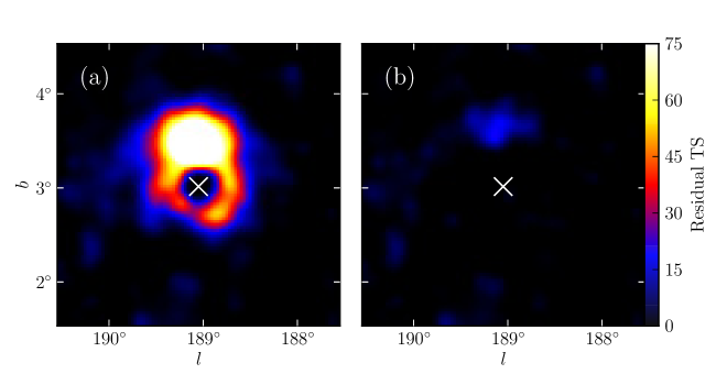
Figure 6.1: A TS map generated for the region around the SNR IC 443 using photons with energies between 1 GeV and 100 GeV. (a) TS map after subtracting IC 443 modeled as a point-like source. (b) same as (a), but IC 443 modeled as an extended source. The cross represents the best fit position of IC 443.

Similarly, many of these sources were confused with nearby point-like sources or influenced by large-scale residuals in the diffuse emission. To help determine which of these fits found truly extended sources and when the extension was influenced by source confusion and diffuse emission, we generated a series of diagnostic plots. For each candidate, we generated a map of the residual TS by adding a new point-like source of spectral index 2 into the region at each position and finding the increase in likelihood when fitting its flux. Figure 6.1 shows this map around the most significantly extended source IC 443 when it is modeled both as a point-like source and as an extended source. The residual TS map indicates that the spatially extended model for IC 443 is a significantly better description of the observed photons and that there is no $\mathrm{TS}>25$ residual in the region after modeling the source as being spatially extended. We also generated plots of the sum of all counts within a given distance of the source and compared them to the model predictions assuming the emission originated from a point-like source. An example radial integral plot is shown for the extended source IC 443 in Figure 5.1. For each source, we also made diffuse-emission-subtracted smoothed counts maps (shown for IC 443 in Figure 5.1).

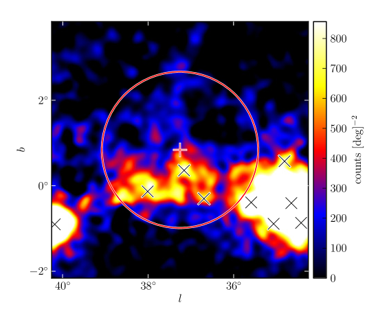
Figure 6.2: A diffuse-emission-subtracted 1 GeV to 100 GeV counts map of the region around 2FGL J1856.2+0450c smoothed by a 0$.\!\!^{\circ}$1 2D Gaussian kernel. The plus-shaped marker and circle (colored red in the online version) represent the center and size of the source fit with a radially-symmetric uniform disk spatial model. The black crosses represent the positions of other 2FGL sources. The extension is statistically significant, but the extension encompasses many 2FGL sources and the emission does not look to be uniform. Although the fit is statistically significant, it likely corresponds to residual features of inaccurately modeled diffuse emission picked up by the fit.

We found by visual inspection that in many cases our results were strongly influenced by large-scale residuals in the diffuse emission and hence the extension measure was unreliable. This was especially true in our analysis of sources in the 1 GeV to 100 GeV energy range. An example of such a case is 2FGL J1856.2+0450c analyzed in the 1 GeV to 100 GeV energy range. Figure 6.2 shows a diffuse-emission-subtracted smoothed counts map for this source with the best fit extension of the source overlaid. There appear to be large-scale residuals in the diffuse emission in this region along the Galactic plane. As a result, 2FGL J1856.2+0450c is fit to an extension of $\sim 2^{\circ}$ and the result is statistically significant with $\mathrm{TS}_{\mathrm{ext}}$ =45.4. However, by looking at the residuals it is clear that this complicated region is not well modeled. We manually discard sources like this.

We only selected extended source candidates in regions that did not appear dominated by these issues and where there was a multiwavelength counterpart. Because of these systematic issues, this search can not be expected to be complete and it is likely that there are other spatially extended sources that this method missed.

Table 6.2: Nearby Residual-induced Sources

Extended Source	Residual-induced Sources
2FGL J0823.0$-$4246	2FGL J0821.0$-$4254, 2FGL J0823.4$-$4305
2FGL J1627.0$-$2425c
2FGL J0851.7$-$4635	2FGL J0848.5$-$4535, 2FGL J0853.5$-$4711, 2FGL J0855.4$-$4625
2FGL J1615.0$-$5051
2FGL J1615.2$-$5138	2FGL J1614.9$-$5212
2FGL J1632.4$-$4753c	2FGL J1634.4$-$4743c
2FGL J1712.4$-$3941
2FGL J1837.3$-$0700c	2FGL J1835.5$-$0649
2FGL J2021.5+4026	2FGL J2019.1+4040

Note. — For each new extended source, we list nearby 2FGL soruces that we have concluded here correspond to residuals induced by not modeling the extensions of nearby extended sources.

For each candidate that was not biased by neighboring point-like sources or by large-scale residuals in the diffuse emission model, we improved the model of the region by deciding on a case by case basis which background point-like sources should be kept. We kept in our model the sources that we believed represented physically distinct sources and we removed sources that we believed were included in the 2FGL catalog to compensate for residuals induced by not modeling the extension of the source. Soft nearby point-like 2FGL sources that were not significant at higher energies were frozen to the spectras predicted by 2FGL. When deciding which background sources to keep and which to remove, we used multiwavelength information about possibly extended source counterparts to help guide our choice. For each extended source presented in Section 6.4, we describe any modifications from 2FGL of the background model that were performed. In Table 6.2, we summarize the sources in the 2FGL catalog that we have concluded here correspond to residuals induced by not modeling the extensions of nearby extended sources.

The best fit positions of nearby point-like sources can be influenced by the extended source and vice versa. Similarly, the best fit positions of nearby point-like sources in the 2FGL catalog can be biased by systematic issues at lower energies. Therefore, after selecting the list of background sources, we iteratively refit the positions and spectra of nearby background sources as well as the positions and extensions of the analyzed spatially extended sources until the overall fit converged globally. For each extended source, we will describe the positions of any relocalized background sources.

After obtaining the overall best fit positions and extensions of all of the sources in the region using $\mathtt{pointlike}$, we refit the spectral parameters of the region using $\mathtt{gtlike}$. With $\mathtt{gtlike}$, we obtained a second measure of $\mathrm{TS}_{\mathrm{ext}}$. We only consider a source to be extended when both $\mathtt{pointlike}$ and $\mathtt{gtlike}$ agree that $\mathrm{TS}_{\mathrm{ext}}\geq 16$. We further required that $\mathrm{TS}_{\mathrm{ext}}\geq 16$ using the alternative approach to modeling the diffuse emission presented in Section 6.2. We then replaced the spatially extended source with two point-like sources and refit the positions and spectra of the two point-like sources to calculate $\mathrm{TS}_{\mathrm{2pts}}$. We only consider a source to be spatially extended, instead of being the result of confusion of two point-like sources, if $\mathrm{TS}_{\mathrm{ext}}>\mathrm{TS}_{\mathrm{2pts}}$. As was shown in Section 5.5, this test is fairly powerful at removing situations in which the emission actually originates from two distinct point-like sources instead of one spatially extended source. On the other hand, it is still possible that longer observations could resolve additional structure or new sources that the analysis cannot currently detect. Considering the very complicated morphologies of extended sources observed at other wavelengths and the high density of possible sources that are expected to emit at GeV energies, it is likely that in some of these regions further observations will reveal that the emission is significantly more complicated than the simple radially-symmetric uniform disk model that we assume.

6.4 New Extended Sources

Table 6.3: Extension fit for the nine additional extended sources

Name	GLON	GLAT	$\sigma$	$\mathrm{TS}$	$\mathrm{TS}_{\mathrm{ext}}$	Pos Err	Flux	Index	Counterpart
	(deg.)	(deg.)	(deg.)			(deg.)
E$>$1 GeV
2FGL J0823.0$-$4246	260.32	$-$3.28	$0.37\pm 0.03\pm 0.02$	322.2	48.0	0.02	$8.4\pm 0.6$	$2.21\pm 0.09$	Puppis A
2FGL J1627.0$-$2425c	353.07	16.80	$0.42\pm 0.05\pm 0.16$	139.9	32.4	0.04	$6.3\pm 0.6$	$2.50\pm 0.14$	Ophiuchus
E$>$10 GeV
2FGL J0851.7$-$4635	266.31	$-$1.43	$1.15\pm 0.08\pm 0.02$	116.6	86.8	0.07	$1.3\pm 0.2$	$1.74\pm 0.21$	Vela Jr.
2FGL J1615.0$-$5051	332.37	$-$0.13	$0.32\pm 0.04\pm 0.01$	50.4	16.7	0.04	$1.0\pm 0.2$	$2.19\pm 0.28$	HESS J1616$-$508
2FGL J1615.2$-$5138	331.66	$-$0.66	$0.42\pm 0.04\pm 0.02$	76.1	46.5	0.04	$1.1\pm 0.2$	$1.79\pm 0.26$	HESS J1614$-$518
2FGL J1632.4$-$4753c	336.52	0.12	$0.35\pm 0.04\pm 0.02$	64.4	26.9	0.04	$1.4\pm 0.2$	$2.66\pm 0.30$	HESS J1632$-$478
2FGL J1712.4$-$3941	347.26	$-$0.53	$0.56\pm 0.04\pm 0.02$	59.4	38.5	0.05	$1.2\pm 0.2$	$1.87\pm 0.22$	RX J1713.7$-$3946
2FGL J1837.3$-$0700c	25.08	0.13	$0.33\pm 0.07\pm 0.05$	47.0	18.5	0.07	$1.0\pm 0.2$	$1.65\pm 0.29$	HESS J1837$-$069
2FGL J2021.5+4026	78.24	2.20	$0.63\pm 0.05\pm 0.04$	237.2	128.9	0.05	$2.0\pm 0.2$	$2.42\pm 0.19$	$\gamma$-Cygni

Note. — The columns in this table have the same meaning as those in Table 6.1. RX J1713.7$-$3946 and Vela Jr. were previously studied in dedicated publications (Abdo et al. 2011b; Tanaka et al. 2011).

Table 6.4: Dual localization, alternative PSF, and alternative approach to modeling the diffuse emission

Name	$\mathrm{TS}_{\mathtt{pointlike}}$	$\mathrm{TS}_{\mathtt{gtlike}}$	$\mathrm{TS}_{\text{alt,diff}}$	${\mathrm{TS}_{\mathrm{ext}}}_{,\mathtt{pointlike}}$	${\mathrm{TS}_{\mathrm{ext}}}_{,\mathtt{gtlike}}$	${\mathrm{TS}_{\mathrm{ext}}}_{\text{alt,diff}}$	$\sigma$	$\sigma_{\text{alt,diff}}$	$\sigma_{\text{alt,psf}}$	$\mathrm{TS}_{\mathrm{2pts}}$
							(deg.)	(deg.)	(deg.)
E$>$1 GeV
2FGL J0823.0$-$4246	331.9	322.2	356.0	60.0	48.0	56.0	0.37	0.39	0.39	23.0
2FGL J1627.0$-$2425c	154.8	139.9	105.7	39.4	32.4	24.8	0.42	0.40	0.58	24.5
E$>$10 GeV
2FGL J0851.7$-$4635	115.2	116.6	123.1	83.9	86.8	89.8	1.15	1.16	1.17	15.5
2FGL J1615.0$-$5051	48.2	50.4	56.6	15.2	16.7	17.8	0.32	0.33	0.32	13.1
2FGL J1615.2$-$5138	75.0	76.1	83.8	42.9	46.5	54.1	0.42	0.43	0.43	35.1
2FGL J1632.4$-$4753c	64.5	64.4	66.8	23.0	26.9	25.5	0.35	0.36	0.37	10.9
2FGL J1712.4$-$3941	59.8	59.4	39.9	38.4	38.5	30.7	0.56	0.55	0.53	2.7
2FGL J1837.3$-$0700c	44.5	47.0	39.2	17.6	18.5	16.1	0.33	0.32	0.38	10.8
2FGL J2021.5+4026	239.1	237.2	255.8	139.1	128.9	138.0	0.63	0.65	0.59	37.3

Note. — $\mathrm{TS}_{\mathtt{pointlike}}$, $\mathrm{TS}_{\mathtt{gtlike}}$, and $\mathrm{TS}_{\text{alt,diff}}$ are the test statistic values from $\mathtt{pointlike}$, $\mathtt{gtlike}$, and $\mathtt{gtlike}$ with the alternative approach to modeling the diffuse emission respectively. ${\mathrm{TS}_{\mathrm{ext}}}_{,\mathtt{pointlike}}$, ${\mathrm{TS}_{\mathrm{ext}}}_{,\mathtt{gtlike}}$, and ${\mathrm{TS}_{\mathrm{ext}}}_{\text{alt,diff}}$ are the TS values from $\mathtt{pointlike}$, $\mathtt{gtlike}$, and $\mathtt{gtlike}$ with the alternative approach to modeling the diffuse emission respectively. $\sigma$, $\sigma_{\text{alt,diff}}$, and $\sigma_{\text{alt,psf}}$ are the fit sizes assuming a radially-symmetric uniform disk model with the standard analysis, the alternative approach to modeling the diffuse emission, and the alternative PSF respectively.

Nine extended sources not included in the 2FGL catalog were found by our extended source search. Two of these have been previously studied in dedicated publications: RX J1713.7$-$3946 and Vela Jr. (Abdo et al. 2011b; Tanaka et al. 2011). Two of these sources were found when using photons with energies between 1 GeV and 100 GeV and seven were found when using photons with energies between 10 GeV and 100 GeV. For the sources found at energies above 10 GeV, we restrict our analysis to higher energies because of the issues of source confusion and diffuse emission modeling described in Section 6.3. The spectral and spatial properties of these nine sources are summarized in Table 6.3 and the results of our investigation of systematic errors are presented in Table 6.4. Table 6.4 also compares the likelihood assuming the source is spatially extended to the likelihood assuming that the emission originates from two independent point-like sources. For these new extended sources, $\mathrm{TS}_{\mathrm{ext}}>\mathrm{TS}_{\mathrm{2pts}}$ so we conclude that the GeV emission does not originate from two physically distinct point-like sources (see Section 5.5). Table 6.4 also includes the results of the extension fits using variations of the PSF and the Galactic diffuse model described in Section 6.2. There is good agreement between $\mathrm{TS}_{\mathrm{ext}}$ and the fit size using the standard analysis, the alternative approach to modeling the diffuse emission, and the alternative PSF. This suggests that the sources are robust against mis-modeled features in the diffuse emission model and uncertainties in the PSF.

6.4.1 2FGL J0823.0$-$4246

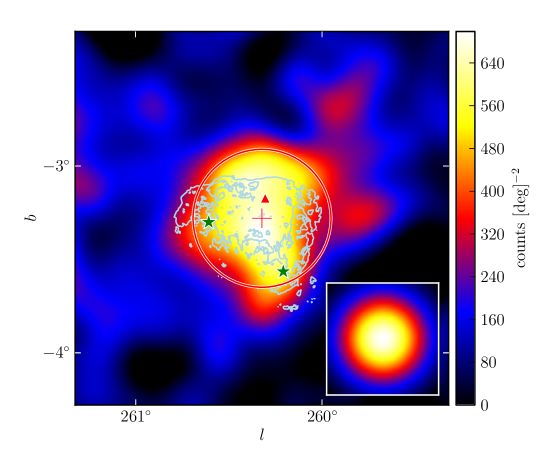
Figure 6.3: A diffuse-emission-subtracted 1 GeV to 100 GeV counts map of 2FGL J0823.0$-$4246 smoothed by a 0$.\!\!^{\circ}$1 2D Gaussian kernel. The triangular marker (colored red in the online version) represents the 2FGL position of this source. The plus-shaped marker and the circle (colored red) represent the best fit position and extension of this source assuming a radially-symmetric uniform disk model. The two star-shaped markers (colored green) represent 2FGL sources that were removed from the background model. From left to right, these sources are 2FGL J0823.4$-$4305 and 2FGL J0821.0$-$4254. The lower right inset is the model predicted emission from a point-like source with the same spectrum as 2FGL J0823.4$-$4305 smoothed by the same kernel. This source is spatially coincident with the Puppis A SNR. The light blue contours correspond to the X-ray image of Puppis A observed by ROSAT (Petre et al. 1996).

2FGL J0823.0$-$4246 was found by our search to be an extended source candidate in the 1 GeV to 100 GeV energy range and is spatially coincident with the SNR Puppis A. Figure 6.3 shows a counts map of this source. There are two nearby 2FGL sources 2FGL J0823.4$-$4305 and 2FGL J0821.0$-$4254 that are also coincident with the SNR but that do not appear to represent physically distinct sources. We conclude that these nearby point-like sources were included in the 2FGL catalog to compensate for residuals induced by not modeling the extension of this source and removed them from our model of the sky. After removing these sources, 2FGL J0823.0$-$4246 was found to have an extension $\sigma=0\mbox{$.\!\!^{\circ}$}37\pm 0\mbox{$.\!\!^{\circ}$}03_{\text{stat}}\pm 0\mbox{$.\!\!^{\circ}$}02_{\text{sys}}$ with $\mathrm{TS}_{\mathrm{ext}}=48.0$. Figure 6.12 shows the spectrum of this source.

Puppis A has been studied in detail in radio (Castelletti et al. 2006), and X-ray (Petre et al. 1996; Hwang et al. 2008). The fit extension of 2FGL J0823.0$-$4246 matches well the size of Puppis A in X-ray. The distance of Puppis A was estimated at 2.2 kpc (Reynoso et al. 1995, 2003) and leads to a 1 GeV to 100 GeV luminosity of $\sim 3\times 10^{34}$ ergs$\,\text{s}^{-1}$. No molecular clouds have been observed directly adjacent to Puppis A (Paron et al. 2008), similar to the LAT-detected Cygnus Loop SNR (Katagiri et al. 2011). The luminosity of Puppis A is also smaller than that of other SNRs believed to interact with molecular clouds (Abdo et al. 2009d, 2010b, 2010a, 2010f, 2010).

6.4.2 2FGL J0851.7$-$4635

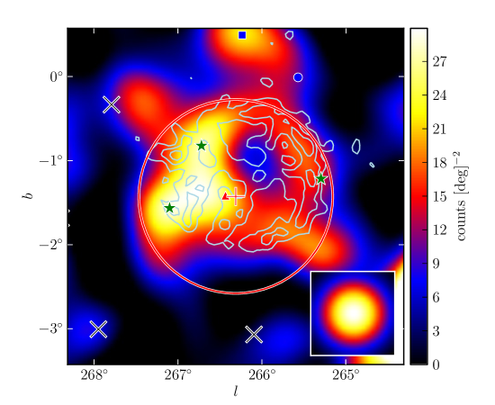
Figure 6.4: A diffuse-emission-subtracted 10 GeV to 100 GeV counts map of 2FGL J0851.7$-$4635 smoothed by a 0$.\!\!^{\circ}$25 2D Gaussian kernel. The triangular marker (colored red in the electronic version) represents the 2FGL position of this source. The plus-shaped marker and the circle (colored red) are the best fit position and extension of this source assuming a radially-symmetric uniform disk model. The three black crosses represent background 2FGL sources. The three star-shaped markers (colored green) represent other 2FGL sources that were removed from the background model. They are (from left to right) 2FGL J0853.5$-$4711, 2FGL J0855.4$-$4625, and 2FGL J0848.5$-$4535. The circular and square-shaped marker (colored blue) represents the 2FGL and relocalized position of another 2FGL source. This extended source is spatially coincident with the Vela Jr. SNR. The contours (colored light blue) correspond to the TeV image of Vela Jr. (Aharonian et al. 2007c).

2FGL J0851.7$-$4635 was found by our search to be an extended source candidate in the 10 GeV to 100 GeV energy range and is spatially coincident with the SNR Vela Jr. This source was recently studied by the LAT Collaboration in Tanaka et al. (2011). Figure 6.4 shows a counts map of the source. Overlaid on Figure 6.4 are TeV contours of Vela Jr. (Aharonian et al. 2007c). There are three point-like 2FGL sources 2FGL J0848.5$-$4535, 2FGL J0853.5$-$4711, and 2FGL J0855.4$-$4625 which correlate with the multiwavelength emission of this SNR but do not appear to be physically distinct sources. They were most likely included in the 2FGL catalog to compensate for residuals induced by not modeling the extension of Vela Jr. and were removed from our model of the sky.

With this model of the background, 2FGL J0851.7$-$4635 was found to have an extension of $\sigma=1\mbox{$.\!\!^{\circ}$}15\pm 0\mbox{$.\!\!^{\circ}$}08_{\text{stat}}\pm 0\mbox{$.\!\!^{\circ}$}02_{\text{sys}}$ with $\mathrm{TS}_{\mathrm{ext}}=86.8$. The LAT size matches well the TeV morphology of Vela Jr. While fitting the extension of 2FGL J0851.7$-$4635, we iteratively relocalized the position of the nearby point-like 2FGL source 2FGL J0854.7$-$4501 to $(l,b)=(266\mbox{$.\!\!^{\circ}$}24,0\mbox{$.\!\!^{\circ}$}49)$ to better fit its position at high energies.

6.4.3 2FGL J1615.0$-$5051

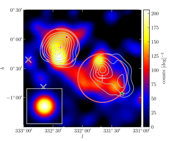
Figure 6.5: A diffuse-emission-subtracted 10 GeV to 100 GeV counts map of 2FGL J1615.0$-$5051 (upper left) and 2FGL J1615.2$-$5138 (lower right) smoothed by a 0$.\!\!^{\circ}$1 2D Gaussian kernel. The triangular markers (colored red in the electronic version) represent the 2FGL positions of these sources. The cross-shaped markers and the circles (colored red) represent the best fit positions and extensions of these sources assuming a radially symmetric uniform disk model. The two black crosses represent background 2FGL sources and the star-shaped marker (colored green) represents 2FGL J1614.9-5212, another 2FGL source that was removed from the background model. The contours (colored light blue) correspond to the TeV image of HESS J1616$-$508 (left) and HESS J1614$-$518 (right) (Aharonian et al. 2006e).

2FGL J1615.0$-$5051 and 2FGL J1615.2$-$5138 were both found to be extended source candidates in the 10 GeV to 100 GeV energy range. Because they are less than $1^{\circ}$ away from each other, they needed to be analyzed simultaneously. 2FGL J1615.0$-$5051 is spatially coincident with the extended TeV source HESS J1616$-$508 and 2FGL J1615.2$-$5138 is coincident with the extended TeV source HESS J1614$-$518. Figure 6.5 shows a counts map of these sources and overlays the TeV contours of HESS J1616$-$508 and HESS J1614$-$518 (Aharonian et al. 2006e). The figure shows that the 2FGL source 2FGL J1614.9$-$5212 is very close to 2FGL J1615.2$-$5138 and correlates with the same extended TeV source as 2FGL J1615.2$-$5138. We concluded that this source was included in the 2FGL catalog to compensate for residuals induced by not modeling the extension of 2FGL J1615.2$-$5138 and removed it from our model of the sky.

With this model of the sky, we iteratively fit the extensions of 2FGL J1615.0$-$5051 and 2FGL J1615.2$-$5138. 2FGL J1615.0$-$5051 was found to have an extension $\sigma=0\mbox{$.\!\!^{\circ}$}32\pm 0\mbox{$.\!\!^{\circ}$}04_{\text{stat}}\pm 0\mbox{$.\!\!^{\circ}$}01_{\text{sys}}$ and $\mathrm{TS}_{\mathrm{ext}}$ =16.7.

The TeV counterpart of 2FGL J1615.0$-$5051 was fit with a radially-symmetric Gaussian surface brightness profile with $\sigma=0\mbox{$.\!\!^{\circ}$}136\pm 0\mbox{$.\!\!^{\circ}$}008$ (Aharonian et al. 2006e). This TeV size corresponds to a 68% containment radius of ${\mathrm{r}_{68}}=0\mbox{$.\!\!^{\circ}$}21\pm 0\mbox{$.\!\!^{\circ}$}01$, comparable to the LAT size ${\mathrm{r}_{68}}=0\mbox{$.\!\!^{\circ}$}26\pm 0\mbox{$.\!\!^{\circ}$}03$. Figure 6.8 shows that the spectrum of 2FGL J1615.0$-$5051 at GeV energies connects to the spectrum of HESS J1616$-$508 at TeV energies.

HESS J1616$-$508 is located in the region of two SNRs RCW103 (G332.4-04) and Kes 32 (G332.4+0.1) but is not spatially coincident with either of them (Aharonian et al. 2006e). HESS J1616$-$508 is near three pulsars PSR J1614$-$5048, PSR J1616$-$5109, and PSR J1617$-$5055. (Torii et al. 1998; Landi et al. 2007a). Only PSR J1617$-$5055 is energetically capable of powering the TeV emission and Aharonian et al. (2006e) speculated that HESS J1616$-$508 could be a PWN powered by this young pulsar. Because HESS J1616$-$508 is $9\mbox{${}^{\prime}$}$ away from PSR J1617$-$5055, this would require an asymmetric X-ray PWNe to power the TeV emission. Chandra ACIS observations revealed an underluminous PWN of size $\sim 1\mbox{${}^{\prime}$}$ around the pulsar that was not oriented towards the TeV emission, rendering this association uncertain (Kargaltsev et al. 2008). No other promising counterparts were observed at X-ray and soft $\gamma$-ray energies by Suzaku (Matsumoto et al. 2007), Swift/XRT, IBIS/ISGRBI, BeppoSAX and XMM-Newton (Landi et al. 2007a). Kargaltsev et al. (2008) discovered additional diffuse emission towards the center of HESS J1616$-$508 using archival radio and infared observations. Deeper observations will likely be necessary to understand this $\gamma$-ray source.

6.4.4 2FGL J1615.2$-$5138

2FGL J1615.2$-$5138 was found to have an extension $\sigma=0\mbox{$.\!\!^{\circ}$}42\pm 0\mbox{$.\!\!^{\circ}$}04_{\text{stat}}\pm 0.02_{\text{sys}}$ with $\mathrm{TS}_{\mathrm{ext}}=46.5$. To test for the possibility that 2FGL J1615.2$-$5138 is not spatially extended but instead composed of two point-like sources (one of them represented in the 2FGL catalog by 2FGL J1614.9$-$5212), we refit 2FGL J1615.2$-$5138 as two point-like sources. Because $\mathrm{TS}_{\mathrm{2pts}}=35.1$ is less than $\mathrm{TS}_{\mathrm{ext}}=46.5$, we conclude that this emission does not originate from two closely-spaced point-like sources.

2FGL J1615.2$-$5138 is spatially coincident with the extended TeV source HESS J1614$-$518. H.E.S.S. measured a 2D Gaussian extension of $\sigma=0\mbox{$.\!\!^{\circ}$}23\pm 0\mbox{$.\!\!^{\circ}$}02$ and $\sigma=0\mbox{$.\!\!^{\circ}$}15\pm 0\mbox{$.\!\!^{\circ}$}02$ in the semi-major and semi-minor axis. This corresponds to a 68% containment size of ${\mathrm{r}_{68}}=0\mbox{$.\!\!^{\circ}$}35\pm 0\mbox{$.\!\!^{\circ}$}03$ and $0\mbox{$.\!\!^{\circ}$}23\pm 0\mbox{$.\!\!^{\circ}$}03$, consistent with the LAT size ${\mathrm{r}_{68}}=0\mbox{$.\!\!^{\circ}$}34\pm 0\mbox{$.\!\!^{\circ}$}03$. Figure 6.8 shows that the spectrum of 2FGL J1615.2$-$5138 at GeV energies connects to the spectrum of HESS J1614$-$518 at TeV energies. Further data collected by H.E.S.S. in 2007 resolve a double peaked structure at TeV energies but no spectral variation across this source, suggesting that the emission is not the confusion of physically separate sources (Rowell et al. 2008). This double peaked structure is also hinted at in the LAT counts map in Figure 6.5 but is not very significant. The TeV source was also detected by CANGAROO-III (Mizukami et al. 2011).

There are five nearby pulsars, but none are luminous enough to provide the energy output required to power the $\gamma$-ray emission (Rowell et al. 2008). HESS J1614$-$518 is spatially coincident with a young open cluster Pismis 22 (Landi et al. 2007b; Rowell et al. 2008). Suzaku detected two promising X-ray candidates. Source A is an extended source consistent with the peak of HESS J1614$-$518 and source B coincident with Pismis 22 and towards the center but in a relatively dim region of HESS J1614$-$518 (Matsumoto et al. 2008). Three hypotheses have been presented to explain this emission: either source A is an SNR powering the $\gamma$-ray emission; source A is a PWN powered by an undiscovered pulsar in either source A or B; and finally that the emission may arise from hadronic acceleration in the stellar winds of Pismis 22 (Mizukami et al. 2011).

6.4.5 2FGL J1627.0$-$2425c

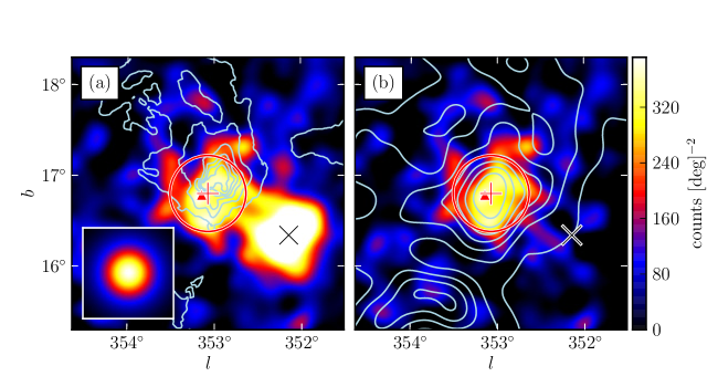
Figure 6.6: A diffuse-emission-subtracted 1 GeV to 100 GeV counts map of (a) the region around 2FGL J1627.0$-$2425 smoothed by a 0$.\!\!^{\circ}$1 2D Gaussian kernel and (b) with the emission from 2FGL J1625.7$-$2526 subtracted. The triangular marker (colored red in the online version) represents the 2FGL position of this source. The plus-shaped marker and the circle (colored red) represent the best fit position and extension of this source assuming a radially-symmetric uniform disk model and the black cross represents a background 2FGL source. The contours in (a) correspond to the 100 $\mu$m image observed by IRAS (Young et al. 1986). The contours in (b) correspond to CO ($J=1\rightarrow 0$) emission integrated from $-$8 $\text{km}\,\text{s}^{-1}$ to 20 $\text{km}\,\text{s}^{-1}$. They are from de Geus et al. (1990), were cleaned using the moment-masking technique (Dame 2011), and have been smoothed by a 0$.\!\!^{\circ}$25 2D Gaussian kernel.

2FGL J1627.0$-$2425c was found by our search to have an extension $\sigma=0\mbox{$.\!\!^{\circ}$}42\pm 0\mbox{$.\!\!^{\circ}$}05_{\text{stat}}\pm 0\mbox{$.\!\!^{\circ}$}16_{\text{sys}}$ with $\mathrm{TS}_{\mathrm{ext}}=32.4$ using photons with energies between 1 GeV and 100 GeV. Figure 6.6 shows a counts map of this source.

This source is in a region of remarkably complicated diffuse emission. Even though it is $16^{\circ}$ from the Galactic plane, this source is on top of the core of the Ophiuchus molecular cloud which contains massive star-forming regions that are bright in infrared. The region also has abundant molecular and atomic gas traced by CO and H I and significant dark gas found only by its association with dust emission (Grenier et al. 2005). Embedded star-forming regions make it even more challenging to measure the column density of dust. Infared and CO ($J=1\rightarrow 0$) contours are overlaid on Figure 6.6 and show good spatial correlation with the GeV emission (Young et al. 1986; de Geus et al. 1990). This source might represent $\gamma$-ray emission from the interactions of cosmic rays with interstellar gas which has not been accounted for in the LAT diffuse emission model.

6.4.6 2FGL J1632.4$-$4753c

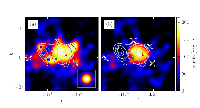
Figure 6.7: A diffuse-emission-subtracted 10 GeV to 100 GeV counts map of 2FGL J1632.4$-$4753c (a) smoothed by a 0$.\!\!^{\circ}$1 2D Gaussian kernel and (b) with the emission from the background sources subtracted. The triangular marker (colored red in the electronic version) represents the 2FGL position of this source. The plus-shaped marker and the circle (colored red) are the best fit position and extension of 2FGL J1632.4$-$4753c assuming a radially-symmetric uniform disk model. The four black crosses represent background 2FGL sources subtracted in (b). The circular and square-shaped markers (colored blue) represent the 2FGL and relocalized positions respectively of two additional background 2FGL sources subtracted in (b). The star-shaped marker (colored green) represents 2FGL J1634.4$-$4743c, another 2FGL source that was removed from the background model. The contours (colored light blue) correspond to the TeV image of HESS J1632$-$478 (Aharonian et al. 2006e).

2FGL J1632.4$-$4753c was found by our search to be an extended source candidate in the 10 GeV to 100 GeV energy range but is in a crowded region of the sky. It is spatially coincident with the TeV source HESS J1632$-$478. Figure 6.7a shows a counts map of this source and overlays TeV contours of HESS J1632$-$478 (Aharonian et al. 2006e). There are six nearby point-like 2FGL sources that appear to represent physically distinct sources and were included in our background model: 2FGL J1630.2$-$4752, 2FGL J1631.7$-$4720c, 2FGL J1632.4$-$4820c, 2FGL J1635.4$-$4717c, 2FGL J1636.3$-$4740c, and 2FGL J1638.0$-$4703c. On the other hand, one point-like 2FGL source 2FGL J1634.4$-$4743c correlates with the extended TeV source and at GeV energies does not appear physically separate. It is very close to the position of 2FGL J1632.4$-$4753c and does not show spatially separated emission in the observed photon distribution. We therefore removed this source from our model of the background. Figure 6.7b shows the same region with the background sources subtracted. With this model, 2FGL J1632.4$-$4753c was found to have an extension $\sigma=0\mbox{$.\!\!^{\circ}$}35\pm 0\mbox{$.\!\!^{\circ}$}04_{\text{stat}}\pm 0\mbox{$.\!\!^{\circ}$}02_{\text{sys}}$ with $\mathrm{TS}_{\mathrm{ext}}=26.9$. While fitting the extension of 2FGL J1632.4$-$4753c, we iteratively relocalized 2FGL J1635.4$-$4717c to $(l,b)=(337\mbox{$.\!\!^{\circ}$}23,0\mbox{$.\!\!^{\circ}$}35)$ and 2FGL J1636.3$-$4740c to $(l,b)=(336\mbox{$.\!\!^{\circ}$}97,-0\mbox{$.\!\!^{\circ}$}07)$.

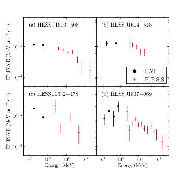
Figure 6.8: The spectral energy distribution of four extended sources associated with unidentified extended TeV sources. The black points with circular markers are obtained by the LAT. The points with plus-shaped markers (colored red in the electronic version) are for the associated H.E.S.S. sources. (a) the LAT SED of 2FGL J1615.0$-$5051 together with the H.E.S.S. SED of HESS J1616$-$508. (b) 2FGL J1615.2$-$5138 and HESS J1614$-$518. (c) 2FGL J1632.4$-$4753c and HESS J1632$-$478. (d) 2FGL J1837.3$-$0700c and HESS J1837$-$069. The H.E.S.S. data points are from (Aharonian et al. 2006e). Both LAT and H.E.S.S. spectral errors are statistical only.

H.E.S.S. measured an extension of $\sigma=0\mbox{$.\!\!^{\circ}$}21\pm 0\mbox{$.\!\!^{\circ}$}05$ and $0\mbox{$.\!\!^{\circ}$}06\pm 0\mbox{$.\!\!^{\circ}$}04$ along the semi-major and semi-minor axes when fitting HESS J1632$-$478 with an elliptical 2D Gaussian surface brightness profile. This corresponds to a 68% containment size ${\mathrm{r}_{68}}=0\mbox{$.\!\!^{\circ}$}31\pm 0\mbox{$.\!\!^{\circ}$}08$ and $0\mbox{$.\!\!^{\circ}$}09\pm 0\mbox{$.\!\!^{\circ}$}06$ along the semi-major and semi-minor axis, consistent with the LAT size ${\mathrm{r}_{68}}=0\mbox{$.\!\!^{\circ}$}29\pm 0\mbox{$.\!\!^{\circ}$}04$. Figure 6.8 shows that the spectrum of 2FGL J1632.4$-$4753c at GeV energies connects to the spectrum of HESS J1632$-$478 at TeV energies.

Aharonian et al. (2006e) argued that HESS J1632$-$478 is positionally coincident with the hard X-ray source IGR J1632$-$4751 observed by ASCA, INTEGRAL, and XMM-Newton (Sugizaki et al. 2001; Tomsick et al. 2003; Rodriguez et al. 2003), but this source is suspected to be a Galactic X-Ray Binary so the $\gamma$-ray extension disfavors the association. Further observations by XMM-Newton discovered point-like emission coincident with the peak of the H.E.S.S. source surrounded by extended emission of size $\sim 32\mbox{${}^{\prime\prime}$}\times 15\mbox{${}^{\prime\prime}$}$ (Balbo et al. 2010). They found in archival MGPS-2 data a spatially coincident extended radio source (Murphy et al. 2007) and argued for a single synchrotron and inverse Compton process producing the radio, X-ray, and TeV emission, likely due to a PWN. The increased size at TeV energies compared to X-ray energies has previously been observed in several aging PWNe including HESS J1825$-$137 (Gaensler et al. 2003; Aharonian et al. 2006c), HESS J1640$-$465 (Aharonian et al. 2006e; Funk et al. 2007), and Vela X (Markwardt & Ogelman 1995; Aharonian et al. 2006d) and can be explained by different synchrotron cooling times for the electrons that produce X-rays and $\gamma$-rays.

6.4.7 2FGL J1712.4$-$3941

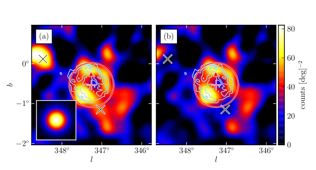
Figure 6.9: A diffuse-emission-subtracted 10 GeV to 100 GeV counts map of 2FGL J1712.4$-$3941 (a) smoothed by a 0$.\!\!^{\circ}$15 2D Gaussian kernel and (b) with the emission from the background sources subtracted. This source is spatially coincident with RX J1713.7$-$3946 and was recently studied in Abdo et al. (2011b). The triangular marker (colored red in the online version) represents the 2FGL position of this source. The plus-shaped marker and the circle (colored red) are the best fit position and extension of this source assuming a radially symmetric uniform disk model. The two black crosses represent background 2FGL sources subtracted in (b). The contours (colored light blue) correspond to the TeV image (Aharonian et al. 2007d).

2FGL J1712.4$-$3941 was found by our search to be spatially extended using photons with energies between 1 GeV and 100 GeV. This source is spatially coincident with the SNR RX J1713.7$-$3946 and was recently studied by the LAT Collaboration in Abdo et al. (2011b). To avoid issues related to uncertainties in the nearby Galactic diffuse emission at lower energy, we restricted our analysis only to energies above 10 GeV. Figure 6.9 shows a smoothed counts map of the source. Above 10 GeV, the GeV emission nicely correlates with the TeV contours of RX J1713.7$-$3946 (Aharonian et al. 2007d) and 2FGL J1712.4$-$3941 fit to an extension $\sigma=0\mbox{$.\!\!^{\circ}$}56\pm 0\mbox{$.\!\!^{\circ}$}04_{\text{stat}}\pm 0\mbox{$.\!\!^{\circ}$}02_{\text{sys}}$ with $\mathrm{TS}_{\mathrm{ext}}=38.5$.

6.4.8 2FGL J1837.3$-$0700c

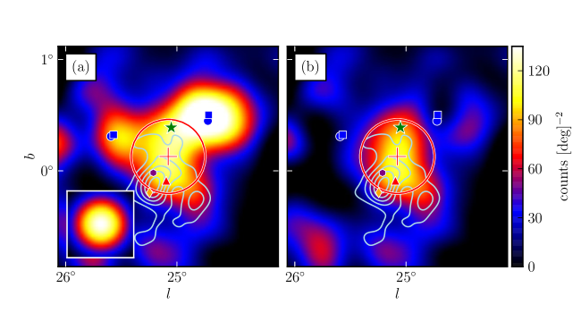
Figure 6.10: A diffuse-emission-subtracted 10 GeV to 100 GeV counts map of the region around 2FGL J1837.3$-$0700c (a) smoothed by a 0$.\!\!^{\circ}$15 2D Gaussian kernel and (b) with the emission from the background sources subtracted. The triangular marker (colored red in the online version) represents the 2FGL position of this source. The plus-shaped marker and the circle (colored red) represent the best fit position and extension of 2FGL J1837.3$-$0700c assuming a radially-symmetric uniform disk model. The circular and square-shaped markers (colored blue) represent the 2FGL and the relocalized positions respectively of two background 2FGL sources subtracted in (b). The star-shaped marker (colored green) represents 2FGL J1835.5$-$0649, another 2FGL source that was removed from the background model. The contours (colored light blue) correspond to the TeV image of HESS J1837$-$069 (Aharonian et al. 2006e). The diamond-shaped marker (colored orange) represents the position of PSR J1838$-$0655 and the hexagonal-shaped marker (colored purple) represents the position AX J1837.3$-$0652 (Gotthelf & Halpern 2008).

2FGL J1837.3$-$0700c was found by our search to be an extended source candidate in the 10 GeV to 100 GeV energy range and is spatially coincident with the TeV source HESS J1837$-$069. This source is in a complicated region. Figure 6.10a shows a smoothed counts map of the region and overlays the TeV contours of HESS J1837$-$069 (Aharonian et al. 2006e). There are two very nearby point-like 2FGL sources, 2FGL J1836.8$-$0623c and 2FGL J1839.3$-$0558c, that clearly represent distinct sources. On the other hand, there is another source 2FGL J1835.5$-$0649 located between the three sources that appears to correlate with the TeV morphology of HESS J1837$-$069 but at GeV energies does not appear to represent a physically distinct source. We concluded that this source was included in the 2FGL catalog to compensate for residuals induced by not modeling the extension of this source and removed it from our model of the sky. Figure 6.10b shows a counts map of this region after subtracting these background sources. After removing 2FGL J1835.5$-$0649, we tested for source confusion by fitting 2FGL J1837.3$-$0700c instead as two point-like sources. Because $\mathrm{TS}_{\mathrm{2pts}}=10.8$ is less than $\mathrm{TS}_{\mathrm{ext}}=18.5$, we conclude that this emission does not originate from two nearby point-like sources.

With this model, 2FGL J1837.3$-$0700c was found to have an extension $\sigma=0\mbox{$.\!\!^{\circ}$}33\pm 0\mbox{$.\!\!^{\circ}$}07_{\text{stat}}\pm 0\mbox{$.\!\!^{\circ}$}05_{\text{sys}}$. While fitting the extension of 2FGL J1837.3$-$0700c, we iteratively relocalized the two closest background sources along with the extension of 2FGL J1837.3$-$0700c but their positions did not significantly change. 2FGL J1834.7$-$0705c moved to $(l,b)=(24\mbox{$.\!\!^{\circ}$}77,0\mbox{$.\!\!^{\circ}$}50)$, 2FGL J1836.8$-$0623c moved to $(l,b)=(25\mbox{$.\!\!^{\circ}$}57,0\mbox{$.\!\!^{\circ}$}32)$.

H.E.S.S. measured an extension of $\sigma=0\mbox{$.\!\!^{\circ}$}12\pm 0\mbox{$.\!\!^{\circ}$}02$ and $0\mbox{$.\!\!^{\circ}$}05\pm 0\mbox{$.\!\!^{\circ}$}02$ of the coincident TeV source HESS J1837$-$069 along the semi-major and semi-minor axis when fitting this source with an elliptical 2D Gaussian surface brightness profile. This corresponds to a 68% containment radius of ${\mathrm{r}_{68}}=0\mbox{$.\!\!^{\circ}$}18\pm 0\mbox{$.\!\!^{\circ}$}03$ and $0\mbox{$.\!\!^{\circ}$}08\pm 0\mbox{$.\!\!^{\circ}$}03$ along the semi-major and semi-minor axis. The size is not significantly different from the LAT 68% containment radius of ${\mathrm{r}_{68}}=0\mbox{$.\!\!^{\circ}$}27\pm 0\mbox{$.\!\!^{\circ}$}07$ (less than $2\sigma$). Figure 6.8 shows that the spectrum of 2FGL J1837.3$-$0700c at GeV energies connects to the spectrum of HESS J1837$-$069 at TeV energies.

HESS J1837$-$069 is coincident with the hard and steady X-ray source AX J1838.0$-$0655 (Bamba et al. 2003). This source was discovered by RXTE to be a pulsar (PSR J1838-0655) sufficiently luminous to power the TeV emission and was resolved by Chandra to be a bright point-like source surrounded by a $\sim 2\mbox{${}^{\prime}$}$ nebula (Gotthelf & Halpern 2008). The $\gamma$-ray emission may be powered by this pulsar. The hard spectral index and spatial extension of 2FGL J1837.3$-$0700c disfavor a pulsar origin of the LAT emission and suggest instead that the GeV and TeV emission both originate from the pulsar’s wind. There is another X-ray point-like source AX J1837.3$-$0652 near HESS J1837$-$069 (Bamba et al. 2003) that was also resolved into a point-like and diffuse component (Gotthelf & Halpern 2008). Although no pulsations have been detected from it, it could also be a pulsar powering some of the $\gamma$-ray emission.

6.4.9 2FGL J2021.5+4026

The source 2FGL J2021.5+4026 is associated with the $\gamma$-Cygni SNR and has been speculated to originate from the interaction of accelerated particles in the SNR with dense molecular clouds (Pollock 1985; Gaisser et al. 1998). This association was disfavored when the GeV emission from this source was detected to be pulsed (PSR J2021+4026, Abdo et al. 2010e). This pulsar was also observed by AGILE (Chen et al. 2011).

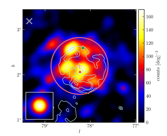
Figure 6.11: A diffuse-emission-subtracted 10 GeV to 100 GeV counts map of the region around 2FGL J2021.5+4026 smoothed by a 0$.\!\!^{\circ}$1 2D Gaussian kernel. The triangular marker (colored red in the online version) represents the 2FGL position of this source. The plus-shaped marker and the circle (colored red) represent the best fit position and extension of 2FGL J2021.5+4026 assuming a radially-symmetric uniform disk model. The star-shaped marker (colored green) represents 2FGL J2019.1+4040, a 2FGL source that was removed from the background model. 2FGL J2021.5+4026 is spatially coincident with the $\gamma$-Cygni SNR. The contours (colored light blue) correspond to the 408MHz image of $\gamma$-Cygni observed by the Canadian Galactic Plane Survey (Taylor et al. 2003).

Looking at the same region at energies above 10 GeV, the pulsar is no longer significant but we instead found in our search an extended source candidate. Figure 6.11 shows a counts map of this source and overlays radio contours of $\gamma$-Cygni from the Canadian Galactic Plane Survey (Taylor et al. 2003). There is good spatial overlap between the SNR and the GeV emission.

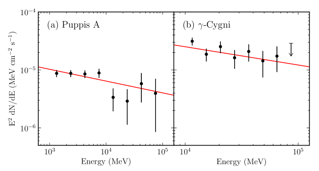
Figure 6.12: The spectral energy distribution of the extended sources Puppis A (2FGL J0823.0$-$4246) and $\gamma$-Cygni (2FGL J2021.5+4026). The lines (colored red in the online version) are the best fit power-law spectral models of these sources. Puppis A has a spectral index of $2.21\pm 0.09$ and $\gamma$-Cygni has an index of $2.42\pm 0.19$. The spectral errors are statistical only. The upper limit is at the 95% confidence level.

There is a nearby source 2FGL J2019.1+4040 that correlates with the radio emission of $\gamma$-Cygni and at GeV energies does not appear to represent a physically distinct source. We concluded that it was included in the 2FGL catalog to compensate for residuals induced by not modeling the extension of $\gamma$-Cygni and removed it from our model of the sky. With this model, 2FGL J2021.5+4026 was found to have an extension $\sigma=0\mbox{$.\!\!^{\circ}$}63\pm 0\mbox{$.\!\!^{\circ}$}05_{\text{stat}}\pm 0\mbox{$.\!\!^{\circ}$}04_{\text{sys}}$ with $\mathrm{TS}_{\mathrm{ext}}=128.9$. Figure 6.12 shows its spectrum. The inferred size of this source at GeV energies well matches the radio size of $\gamma$-Cygni. Milagro detected a $4.2\sigma$ excess at energies $\sim 30$ TeV from this location (Abdo et al. 2009e, f). VERITAS also detected an extended source VER J2019+407 coincident with the SNR above 200 GeV and suggested that the TeV emission could be a shock-cloud interaction in $\gamma$-Cygni (Weinstein & for the VERITAS Collaboration 2009).

6.5 Discussion

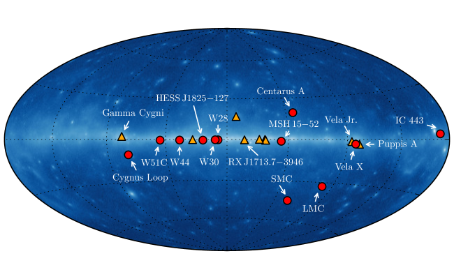
Figure 6.13: The 21 spatially extended sources detected by the LAT at GeV energies with 2 years of data. The twelve extended sources included in 2FGL are represented by the circular markers (colored red in the online version). The nine new extended sources are represented by the triangular markers (colored orange). The source positions are overlaid on a 100 MeV to 100 GeV Aitoff projection sky map of the LAT data in Galactic coordinates.

Twelve extended sources were included in the 2FGL catalog and two additional extended sources were studied in dedicated publications. Using 2 years of LAT data and a new analysis method, we presented the detection of seven additional extended sources. We also reanalyzed the spatial extents of the twelve extended sources in the 2FGL catalog and the two additional sources. The 21 extended LAT sources are located primarily along the Galactic plane and their locations are shown in Figure 6.13. Most of the LAT-detected extended sources are expected to be of Galactic origin as the distances of extragalactic sources (with the exception of the local group Galaxies) are typically too large to be able to resolve them at $\gamma$-ray energies.

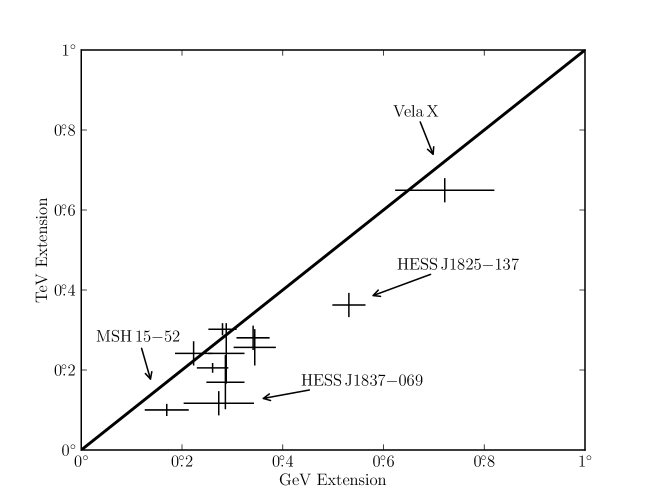
Figure 6.14: A comparison of the sizes of extended sources detected at both GeV and TeV energies. The TeV sizes of W30, 2FGL J1837.3$-$0700c, 2FGL J1632.4$-$4753c, 2FGL J1615.0$-$5051, and 2FGL J1615.2$-$5138 are from Aharonian et al. (2006e). The TeV sizes of MSH 15$-$52, HESS J1825$-$137, Vela X, Vela Jr., RX J1713.7$-$3946 and W28 are from Aharonian et al. (2005a, 2006c, 2006d, 2007c, 2007d, 2008a). The TeV size of IC 443 is from Acciari et al. (2009) and W51C is from Krause et al. (2011). The TeV sizes of MSH 15$-$52, HESS J1614$-$518, HESS J1632$-$478, and HESS J1837$-$069 have only been reported with an elliptical 2D Gaussian fit and so the plotted sizes are the geometric mean of the semi-major and semi-minor axis. The LAT extension of Vela X is from Abdo et al. (2010). The TeV sources were fit assuming a 2D Gaussian surface brightness profile so the plotted GeV and TeV extensions were first converted to $\mathrm{r}_{68}$ (see Section 5.2.4). Because of their large sizes, the shape of RX J1713.7$-$3946 and Vela Jr. were not directly fit at TeV energies and so are not included in this comparison. On the other hand, dedicated publications by the LAT collaboration on these sources showed that their morphologies are consistent (Abdo et al. 2011b; Tanaka et al. 2011). The LAT extension errors are the statistical and systematic errors added in quadrature.

For the LAT extended sources also seen at TeV energies, Figure 6.14 shows that there is a good correlation between the sizes of the sources at GeV and TeV energies. Even so, the sizes of PWNe are expected to vary across the GeV and TeV energy range and the size of HESS J1825$-$137 is significantly larger at GeV than TeV energies (Grondin et al. 2011). It is interesting to compare the sizes of other PWN candidates at GeV and TeV energies, but definitively measuring a difference in size would require a more in-depth analysis of the LAT data using the same elliptical Gaussian spatial model.

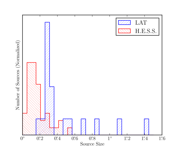
Figure 6.15: The distributions of the sizes of 18 extended LAT sources at GeV energies (colored blue in the electronic version) and the sizes of the 40 extended H.E.S.S. sources at TeV energies (colored red). The H.E.S.S. sources were fit with a 2D Gaussian surface brightness profile so the LAT and H.E.S.S. sizes were first converted to $\mathrm{r}_{68}$. The GeV size of Vela X is taken from Abdo et al. (2010). Because of their large sizes, the shape of RX J1713.7$-$3946 and Vela Jr. were not directly fit at TeV energies and are not included in this comparison. Centaurus A is not included because of its large size.

Figure 6.15 compares the sizes of the 21 extended LAT sources to the 42 extended H.E.S.S. sources. Because of the large field of view and all-sky coverage, the LAT can more easily measure larger sources. On the other hand, the better angular resolution of IACTs allows them to measure a population of extended sources below the resolution limit of the LAT (currently about $\sim 0\mbox{$.\!\!^{\circ}$}2$). Fermi has a 5 year nominal mission lifetime with a goal of 10 years of operation. As Figure 5.10 shows, the low background of the LAT at high energies allows its sensitivity to these smaller sources to improve by a factor greater than the square root of the relative exposures. With increasing exposure, the LAT will likely begin to detect and resolve some of these smaller TeV sources.

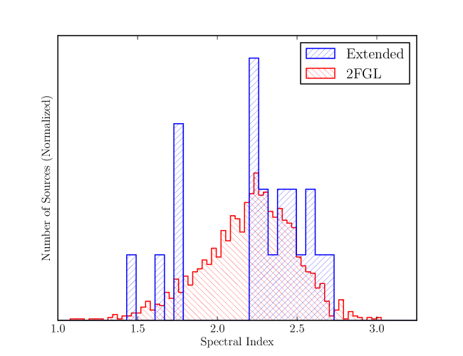
Figure 6.16: The distribution of spectral indices of the 1873 2FGL sources (colored red in the electronic version) and the 21 spatially extended sources (colored blue). The index of Centaurus A is taken from Nolan et al. (2012) and the index of Vela X is taken from Abdo et al. (2010).

Figure 6.16 compares the spectral indices of LAT detected extended sources and of all sources in the 2FGL catalog. This, and Table 6.1 and Table 6.3, show that the LAT observes a population of hard extended sources at energies above 10 GeV. Figure 6.8 shows that the spectra of four of these sources (2FGL J1615.0$-$5051, 2FGL J1615.2$-$5138, 2FGL J1632.4$-$4753c, and 2FGL J1837.3$-$0700c) at GeV energies connects to the spectra of their H.E.S.S. counterparts at TeV energies. This is also true of Vela Jr., HESS J1825$-$137 (Grondin et al. 2011), and RX J1713.7$-$3946 (Abdo et al. 2011b). It is likely that the GeV and TeV emission from these sources originates from the same population of high-energy particles.

Many of the TeV-detected extended sources now seen at GeV energies are currently unidentified and further multiwavelength follow-up observations will be necessary to understand these particle accelerators. Extending the spectra of these TeV sources towards lower energies with LAT observations may help to determine the origin and nature of the high-energy emission.

Chapter 7 Search for PWNe Associated with Gamma-loud Pulsars

This chapter is based on section seven “Unpulsed Magnetospheric Emission” from the paper “The Second Fermi Large Area Telescope Catalog of Gamma-ray Pulsars” (Abdo et al. in prep).

Some pulsars have magnetospheric emission over their full rotation phase with similar spectral characteristics to the emission seen through their peaks. This emission appears in the observed light curves as a low-level, unpulsed component above the estimated background level (i.e., not attributable to diffuse emission or nearby point sources) and can be a powerful discriminator for the emission models.

On the other hand a PWN around the pulsar, or a photon excess due to imprecise knowledge of diffuse emission around the pulsar, would not be modulated at the rotational period and could be confused with a constant magnetospheric signal. Including the discovery of the GeV PWN 3C 58 associated with PSR J0205+6449 described in this section, the LAT sees 17 sources potentially associated with PWNe at GeV energies (Acero et al. in prep.). Some are highlighted in Section 7.4. This off-peak emission should be properly modeled when searching for pulsar emission at all rotation phases.

We can discriminate between these two possible signals through spectral and spatial analysis. If the emission is magnetospheric, it is more likely to appear as a non-variable point source with an exponentially cutoff spectrum with a well-known range of cutoff energies. On the other hand, PWNe and diffuse excesses have spectra with a power-law shape and either a hard index continuing up to tens of GeV in the PWN case or present only at lower energies with a very soft index in the diffuse case. In addition, PWNe are often spatially resolvable at GeV energies (e.g., Vela-X has been spatially resolved with the LAT and AGILE and HESS J1825$-$137 with the LAT; Abdo et al. 2010; Pellizzoni et al. 2010; Grondin et al. 2011, respectively) so an extended source would argue against a magnetospheric origin of the emission. However, given the finite angular resolution of the LAT not all PWNe will appear spatially extended at GeV energies. The Crab Nebula, for instance, cannot be resolved by the LAT but can be distinguished from the gamma-bright Crab pulsar, in the off-peak interval, by its hard spectrum above $\sim$1 GeV (Abdo et al. 2010e). In addition, GeV emission from the Crab Nebula was discovered to be time-variable (e.g., Abdo et al. 2011a) providing another possible way to discern the nature of any observed off-peak signal.

Therefore, to identify pulsars with magnetospheric emission across the entire rotation, we define and search the off-peak intervals of the pulsars in this catalog for significant emission, except PSR J2215+5135 for which the rotation ephemeris covers a short time interval and the profile is noisy. We then evaluate the spectral and spatial characteristics of any off-peak emission to determine if it is likely magnetospheric, related to the pulsar wind, or physically unrelated to the pulsar (e.g., unmodeled diffuse emission).

7.1 Off-peak Phase Selection

We first developed a systematic, model-independent, and computationally-efficient method to define the off-peak interval of a pulsar light curve.

We begin by deconstructing the light curve into simple Bayesian Blocks using the algorithm described in Jackson et al. (2005) and Scargle et al. (2013). We could not apply the Bayesian Block algorithm to the weighted-counts light curves because they do not follow Poisson statistics, required by the algorithm. We therefore use an unweighted-counts light curve in which the angular radius and minimum energy selection have been varied to maximize the H-test statistic. To produce Bayesian Blocks on a periodic light curve, we extend the data over three rotations, by copying and shifting the observed phases to cover the phase range from $-$1 to 2. We do, however, define the final blocks to be between phases 0 and 1. To avoid potential contamination from the trailing or leading edges of the peaks, we reduce the extent of the block by 10% on either side, referenced to the center of the block.

There is one free parameter in the Bayesian Block algorithm called ncp_prior which modifies the probability that the algorithm will divide a block into smaller intervals. We found that, in most cases, setting ncp$\rm{}_{prior}=8$ protects against the Bayesian Block decomposition containing unphysically small blocks. For a few marginally-detected pulsars, the algorithm failed to find more than one block and we had to decrease ncp_prior until the algorithm found a variable light curve. Finally, for a few pulsars the Bayesian-block decomposition of the light curves failed to model weak peaks found by the light-curve fitting method presented in (Abdo et al. in prep) or extended too far into the other peaks. For these pulsars, we conservatively shrink the off-peak region.

For some pulsars, the observed light curve has two well-separated peaks with no significant bridge emission, which leads to two well-defined off-peak intervals. We account for this possibility by finding the second-lowest Bayesian block and accepting it as a second off-peak interval if the emission is consistent with that in the lowest block (at the 99% confidence level) and if the extent of the second block is at least half that of the first block.

Figure 7.1 shows the energy-and-radius optimized light curves, the Bayesian block decompositions, and the off-peak intervals for six pulsars. (Abdo et al. in prep) overlay off-peak intervals over the weighted light curves of several pulsars. The off-peak intervals for all pulsars are given in (Abdo et al. in prep).

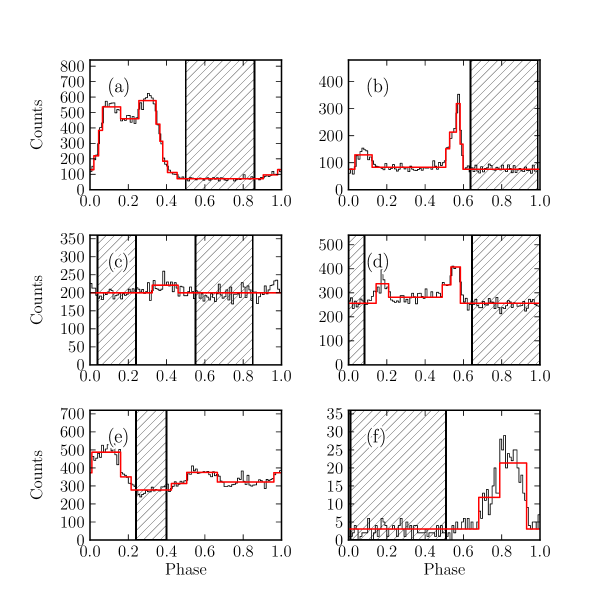
Figure 7.1: The energy-and-radius optimized light curve, Bayesian block decomposition of the light curve, and off-peak interval for (a) PSR J0007+7303, (b) PSR J0205+6449, (c) PSR J1410$-$6132, (d) PSR J1747$-$2958, (e) PSR J2021+4026, and (f) PSR J2124$-$3358. The black histograms represent the light curves, the gray lines (colored red in the electronic version) represent the Bayesian block decompositions of the pulsar light curves, and the hatched areas represent the off-peak intervals selected by this method.

7.2 Off-peak Analysis Method

Characterizing both the spatial and spectral characteristics of any off-peak emission helps discern its origin. We employ a somewhat different analysis procedure here than for the phase-averaged analysis described in (Abdo et al. in prep). To evaluate the spatial characteristics of any off-peak emission we use the likelihood fitting package $\mathtt{pointlike}$ (detailed in Lande et al. 2012), and to fit the spectrum we use $\mathtt{gtlike}$ in binned mode via pyLikelihood as was done for the phase-averaged analysis.

For each pulsar we start from the same temporal and spatial event selections described in (Abdo et al. in prep) but we increase the maximum energy to 400 GeV (the highest event energy for any ROI under this selection is $\sim$316 GeV). For the $\mathtt{pointlike}$ analysis we further select a 10^∘ radius ROI and for $\mathtt{gtlike}$ a $14^{\circ}\times 14^{\circ}$ square ROI, both centered on the pulsar position. Finally, we only consider photons with pulse phases within the corresponding off-peak interval.

We search for off-peak emission assuming a point source and (except for the Crab Nebula and Vela-X, described below) a power-law spectral model. We fit the position of this putative off-peak source using $\mathtt{pointlike}$ as described by Nolan et al. (2012) and then use the best-fit position in a spectral analysis with $\mathtt{gtlike}$. From the spectral analysis we require $TS\geq 25$ (just over $4\sigma$) to claim a detection. If $TS<25$, we compute upper limits on the flux in the energy range from 100 MeV to 316 GeV assuming a power law with photon index fixed to 2.0 and a PLEC1 model with $\Gamma=1.7$ and $E_{\rm cut}=3$ GeV.

The spectrum of the Crab Nebula (associated with PSR J0534+2200) is uniquely challenging because the GeV spectrum contains both a falling synchrotron and a rising inverse Compton component (Abdo et al. 2010e). For this particular source we used the best-fit two-component spectral model from Buehler et al. (2012) and fit only the overall normalization of the source. In addition, for Vela-X (associated with PSR J0835-4510) we took the best-fit spectral model from Grondin et al. (2013) and fit only the overall normalization of this source. This spectrum has a smoothly broken power law spectral model and was fit assuming Vela-X to have an elliptical disk spatial model.

If the off-peak source is significant, we test whether the spectrum shows evidence for a cutoff, as described in Ackermann et al. (2011a), assuming the source is at the pulsar position. We say that the off-peak emission shows evidence for a cutoff if $TS_{\rm cut}\geq 9$, corresponding to a $3\sigma$ detection.

For a significant off-peak point source, we use $\mathtt{pointlike}$ to test if the emission is significantly extended. We assume a radially-symmetric Gaussian source and fit the position and extension parameter ($\sigma$) as described in Lande et al. (2012). The best-fit extended source parameters are then given to $\mathtt{gtlike}$, which is used to fit the spectral parameters and the significance of the extension over a point source, $TS_{\rm ext}$, evaluated as described in Lande et al. (2012). That paper established that $TS_{\rm ext}\geq 16$ means highly probable source extension. In the present work we aim only to flag possible extension, and use $TS_{\rm ext}\geq 9$.

To test for variability, even without significant emission over the 3-year time range, we divide the dataset into 36 intervals and fit the point-source flux independently in each interval, computing $TS_{\rm var}$ as in 2FGL. For sources with potential magnetospheric off-peak emission and for regions with no detection, we performed the test at the pulsar’s position. Otherwise, we test at the best-fit position. The off-peak emission is said to show evidence for variability if $TS_{\rm var}\geq 91.7$, corresponding to a $4\sigma$ significance. As noted in (Abdo et al. in prep), our timing solutions for PSRs J0205+6449 and J1838$-$0537 are not coherent across all three years. For these two pulsars, we excluded the time ranges without ephemerides and only tested for variability during months that were completely covered. For J1838$-$0537 only one month is lost, whereas for J0205+6449 the 7% data loss is spread across three separate months. As a result, $TS_{\rm var}$ for these pulsars is a conservative estimate of variability significance.

The procedure described above, especially the extension analysis, is particularly sensitive to sources not included in 2FGL that are near the pulsar of interest, for two reasons. First, we are using an additional year of data and second, when “turning off” a bright pulsar nearby, faint sources become more important to the global fit. Therefore, in many situations we had to run the analysis several times, iteratively improving the model by including new sources, until we removed all $TS>25$ residuals. The final $\mathtt{gtlike}$-formatted XML source model for each off-peak region is included in the auxiliary material.

There are still, however, pulsars for which we were unable to obtain an unbiased fit of the off-peak emission, most likely due to inaccuracies in the model of the Galactic diffuse emission and incorrectly modeled nearby sources. The most common symptom of a biased fit is an unphysically large extension. In these cases, the extended source attempts to account for multiple point sources or incorrectly-modeled diffuse emission, not just the putative off-peak emission. Systematics associated with modeling extended sources are discussed more thoroughly in Lande et al. (2012). For the purposes of this catalog, we have flagged the pulsars where off-peak analysis suffered from these issues and do not attempt a complete understanding of the emission.

Observations of magnetospheric off-peak emission can be used to constrain pulsar geometry. Therefore, it is important to know if off-peak emission that is otherwise pulsar-like might instead be incorrectly-modeled Galactic diffuse emission. We therefore performed a limited study of the systematics associated with our model of the Galactic diffuse emission.

For sources which otherwise would be classified as magnetospheric, we tested the significance of the emission assuming eight different Galactic diffuse emission models as described in de Palma et al. (2013). These models were constructed using a different model building strategy, vary parameters of the Galactic diffuse emission model, and have additional degrees of freedom in the fit.

We define $\mathrm{TS}_{\text{alt,diff}}$ as the minimum test statistic of any of the eight alternate diffuse models. This test statistic is computed assuming the emission to be pointlike at the best-fit position and is therefore comparable to $\mathrm{TS}_{\mathrm{point}}$. For sources which would otherwise be considered magnetospheric, we flag the emission as potentially spurious if $\mathrm{TS}_{\text{alt,diff}}<25$. We caution that although this test can help to flag problematic regions, these models do not probe the entirety of the uncertainty associated with our model of the Galactic diffuse emission. Therefore, some diffuse emission could still be incorrectly classified as magnetospheric.

7.3 Off-peak Results

The off-peak intervals of 54 LAT-detected pulsars have been evaluated by Ackermann et al. (2011a) using 16 months of sky survey observations. This led to the discovery of PWN-like emission in the off-peak interval of PSR J1023$-$5746, coincident with HESS J1023$-$575, and identification of 5 pulsars that appear to have near 100% duty cycles. Our results, summarized in Table 7.1, extend the analysis to 116 pulsars over 3 years of data. Sample off-peak spectra are shown in Figure 7.2. Using the procedures outlined in Section 7.1 and Section 7.2, we have identified 34 pulsars that have significant emission ($TS\geq 25$) in their off-peak intervals. We classify the likely nature of the emission as follows.

If the emission has $TS_{\rm cut}\geq 9$, we consider the emission to be either magnetospheric (‘M’) or possibly magnetospheric (‘M*’). As was discussed in Section 7.2, we flag the emission as ‘M*’ if the source is formally spatially extended ($TS_{\rm ext}>16$) or if the source is not robust against varying the diffuse emission models ($\mathrm{TS}_{\text{alt,diff}}<25$). On consideration of the angular extent of the PSF of the LAT and inaccuracies in the Galactic diffuse emission model, we caution against considering the ‘M*’ sources to be definitively classified. If the source is significantly cutoff, not significantly extended, and is significant when varying the alternative diffuse models, we classify the emission as ‘M’.

On the other hand, if the emission has $TS_{\rm ext}\geq 16$, and does not suffer from confusion as discussed at the end of Section 7.2, and/or has a hard photon index, we say it is likely to originate in the pulsar wind and identify these sources as type ‘W’. The remaining sources with off-peak emission not satisfying any of the previous criteria are identified as type ‘U’ to indicate that the nature of the emission is unidentified and we do not speculate about its origin.

We identify 9 type ‘M’ sources, significantly expanding the number of pulsars that perhaps have detectable magnetospheric emission across all rotational phases. One caution is that many of these ‘M’ pulsars, especially the young objects, are in regions of particularly bright diffuse gamma-ray emission, where small fractional uncertainties in the level of diffuse emission can account for much of the apparent unpulsed emission. However, if established as true magnetospheric components, these will be important test cases for pulsar emission models. In addition, we identify ten ‘M*’-type regions. For type ‘M’ and ‘M*’ sources, we present the best-fit spectral parameters using a point source at the pulsar’s position with a PLEC1 spectral model in Table 7.1. For all other sources (except the Crab Nebula described in Section 7.2), we present the spectral results using a power-law spectral model and the best-fit spatial representation.

Additionally, we identified four off-peak emissions consistent with a PWN hypothesis, one of them being a new detection at GeV energies (PSR J0205+6449). Only one of these four, the previously identified Vela$-$X PWN (Abdo et al. 2010), is spatially extended for the LAT. Similarly, we detect six type ‘U’ regions. Three of these are formally spatially extended but because of the spatial systematics we assume point-like emission for the spectral analysis.

We mention that for a few sources, the spectral analysis performed here is in disagreement with the analysis presented in Ackermann et al. (2011a). For soft and faint sources (including J1044$-$5737 and J1809$-$2332), the spectral discrepancy is mainly caused by our use of a newer Galactic diffuse model. At lower energies, small changes in the diffuse model can have a significant impact on the analysis of a region. For bright magnetospheric sources (including J0633+1746 and J2021+4026), the spectral discrepancy is mainly due to using different phase ranges (see Section 7.1).

Figure 7.3 shows that only a small fraction of the spindown power goes into the gamma-ray emission from LAT-detected PWNe. Similarly, Abdo et al. (in prep) includes a plot of $\sqrt{\dot{E}}/d^{2}$ vs $\tau_{c}$ which shows that the LAT only detects PWNe from the youngest pulsars with the highest spindown power. GeV emission from the Crab Nebula is highly time variable (Section 7.2). Indeed, we find $TS_{\rm var}=373$ for the Crab Nebula; however no other source demonstrated flux variability (all have $16<TS_{\rm var}<65)$. Other GeV PWNe may be variable, but the combination of lower fluxes and less-extreme variations limits our ability identify them as such.

The off-peak results for several interesting sources are presented in Section 7.4. The complete off-peak search results will be included in the auxiliary information accompanying Abdo et al. (in prep). For regions where we find $TS<25$, the auxiliary information contains upper limits computed for both a power-law spectral model and a PLEC1 model with $E_{\rm cut}=3$ GeV and $\Gamma=1.7$. The auxiliary information also contains $TS_{\rm var}$ for each off-peak interval.

Table 7.1: Off-Peak Spatial and Spectral Results

PSR	Type	$\mathrm{TS}_{\mathrm{point}}$	$\mathrm{TS}_{\mathrm{ext}}$	$\mathrm{TS}_{\mathrm{cutoff}}$	$\mathrm{TS}_{\text{alt,diff}}$	Energy Flux	$\Gamma$	$E_{c}$
						($10^{-11}\,\text{erg}\;\text{cm}^{-2}\text{s}^{-1}$)		(GeV)
Young Pulsars
J0007+7303	U	71.4	10.8	0.0		$1.98\pm 0.26$	$2.61\pm 0.14$
J0205+6449	W	33.7	0.5	0.0		$1.75\pm 0.68$	$1.61\pm 0.21$
J0534+2200	W	5247.	0.0	0.3		$67.2\pm 1.6$
J0631+1036	U	33.1	0.0	5.4		$1.70\pm 0.33$	$2.38\pm 0.14$
J0633+1746	M	3666.	2.3	239.	3369.	$41.4\pm 1.1$	$1.37\pm 0.09$	$0.93\pm 0.10$
J0734$-$1559	M*	28.3	12.4	30.8	0.0	$1.61\pm 0.24$	$0.01\pm 0.08$	$0.17\pm 0.03$
J0835$-$4510	W	473.	283.	22.8		$30.3\pm 1.2$
J0908$-$4913	M*	65.1	41.4	60.4	3.1	$3.04\pm 1.07$	$0.15\pm 0.59$	$0.30\pm 0.01$
J1023$-$5746	M*	59.7	30.0	10.9	72.5	$5.35\pm 1.17$	$0.57\pm 0.80$	$0.49\pm 0.21$
J1044$-$5737	M*	42.0	98.1	22.4	25.6	$3.12\pm 0.75$	$0.80\pm 0.93$	$0.40\pm 0.18$
J1105$-$6107	M*	33.3	37.5	21.7	39.4	$3.81\pm 0.77$	$0.92\pm 0.56$	$0.48\pm 0.22$
J1112$-$6103	U	65.0	71.1	0.9		$5.10\pm 0.74$	$2.17\pm 0.09$
J1119$-$6127	U	61.3	1.0	0.9		$4.11\pm 0.63$	$2.22\pm 0.09$
J1124$-$5916	M	95.9	0.0	18.2	59.4	$2.87\pm 0.71$	$1.31\pm 0.91$	$1.43\pm 1.42$
J1410$-$6132	U	27.5	71.2	0.4		$4.29\pm 1.05$	$1.90\pm 0.15$
J1513$-$5908	W	102.	3.5	0.0		$4.95\pm 0.83$	$1.78\pm 0.12$
J1620$-$4927	M*	28.9	0.5	35.2	0.0	$5.25\pm 0.96$	$0.35\pm 0.94$	$0.57\pm 0.29$
J1746$-$3239	M*	53.3	34.3	34.2	0.0	$3.65\pm 0.59$	$0.94\pm 0.31$	$0.60\pm 0.10$
J1747$-$2958	M	45.5	5.4	49.8	50.4	$8.41\pm 2.84$	$0.02\pm 0.32$	$0.28\pm 0.01$
J1809$-$2332	M*	32.5	13.6	21.9	0.0	$4.10\pm 0.80$	$0.24\pm 0.83$	$0.31\pm 0.11$
J1813$-$1246	M	62.8	0.0	9.0	49.7	$6.31\pm 1.40$	$1.60\pm 0.73$	$0.99\pm 0.95$
J1836+5925	M	10407.	0.0	365.	10401.	$36.9\pm 0.7$	$1.47\pm 0.03$	$1.98\pm 0.09$
J1838$-$0537	M*	51.3	32.9	21.9	41.9	$8.35\pm 1.31$	$1.39\pm 0.54$	$2.55\pm 2.48$
J2021+4026	M	1717.	8.7	244.	1978.	$64.0\pm 1.4$	$1.64\pm 0.02$	$1.82\pm 0.04$
J2032+4127	U	53.6	76.1	1.5		$4.36\pm 0.77$	$2.07\pm 0.12$
J2055+2539	M	123.	0.0	30.0	101.	$1.63\pm 0.19$	$1.05\pm 0.28$	$0.64\pm 0.12$
Millisecond Pulsars
J0034$-$0534	U	41.0	0.0	6.0		$0.82\pm 0.16$	$2.40\pm 0.19$
J0102+4839	U	49.7	0.0	7.4		$1.29\pm 0.20$	$2.51\pm 0.14$
J0218+4232	U	50.1	0.0	6.8		$2.13\pm 0.33$	$2.72\pm 0.26$
J0340+4130	M*	26.9	0.1	16.3	11.9	$0.53\pm 0.11$	$0.02\pm 0.22$	$0.94\pm 0.28$
J1658$-$5324	U	42.3	0.0	1.9		$1.69\pm 0.29$	$2.52\pm 0.76$
J2043+1711	U	52.5	0.0	8.8		$1.46\pm 0.27$	$2.29\pm 0.14$
J2124$-$3358	M	129.	0.0	19.8	118.	$1.08\pm 0.15$	$0.70\pm 0.51$	$1.21\pm 0.49$
J2302+4442	M	114.	0.0	9.8	105.	$1.45\pm 0.20$	$1.54\pm 0.40$	$1.61\pm 0.82$

Note. — Off-peak regions with a significant detection of emission. The source classification is ‘M’ for likely magnetospheric, ‘M*’ for possibly magnetospheric but with a problematic spatial analysis or in a region with possibly poorly-modeled Galactic diffuse emission, ‘W’ for likely pulsar wind, and ‘U’ for unidentified. The table includes the significance of the source ($TS$), of the source extension ($TS_{\rm ext}$), of a spectral cutoff ($TS_{\rm cut}$), and with the alternative diffuse models ($\mathrm{TS}_{\text{alt,diff}}$). The best-fit energy flux and photon index are computed in the energy range from 100 MeV to 316 GeV. For sources with large $TS_{\rm cut}$, the exponential cutoff energies are presented. The quoted errors are statistical only. A few sources are discussed in Section 7.4.

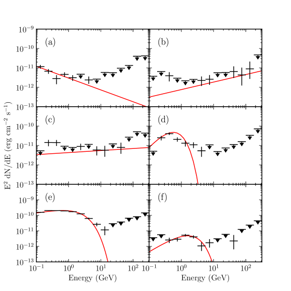
Figure 7.2: Spectral energy distributions for the off-peak phase intervals around (a) PSR J0007+7303 (b) PSR J0205+6449, (c) PSR J1410$-$6132, (d) PSR J1747$-$2958, (e) PSR J2021+4026, and (f) PSR J2124$-$3358. We plot a detection in those energy bands in which the source is found with $TS\geq 4$ (a $2\sigma$ detection) and report a Bayesian 95% confidence-level upper limit otherwise. The best-fit spectral model, using the full energy range, is also shown for comparison.

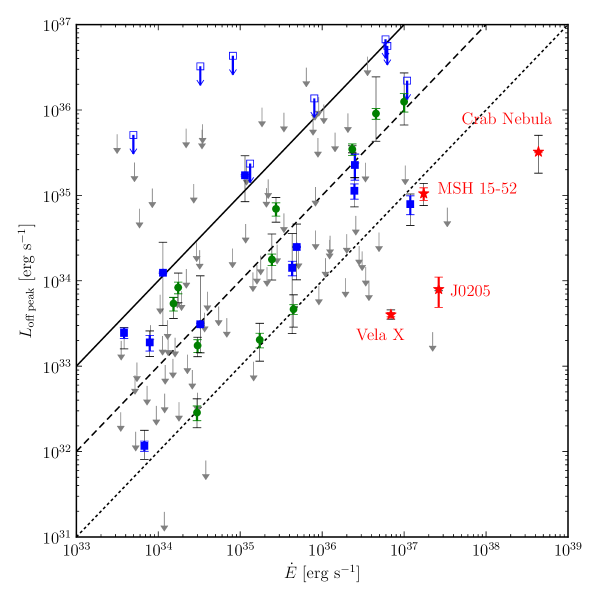
Figure 7.3: The off-peak luminosity compared to the observed pulsar spindown power. The luminosity is computed and plotted with the same convention as luminosities in Abdo et al. (in prep). A luminosity upper limit is plotted when there is no significant off-peak emission or when there is only a distance upper limit. The star-shaped markers (colored red in the online version) represent type ‘W’ sources, the square-shaped markers (colored blue) represent type ‘M’ and ‘M*’ sources, circular markers (colored green) represent type ‘U’ sources, and the gray arrows represent non-detections. The filled blue square-shaped markers represent ‘M’ and ‘M*’ sources with a detected luminosity and the unfilled markers represent luminosity upper limits where there is only a distance upper limit. The solid, dashed, and dotted diagonals show 100%, 10%, and 1% efficiency (respectively).

7.4 Off-Peak Individual Source Discussion

Here we discuss several interesting sources found in the off-peak analysis.

The off-peak emission from PSR J0007+7303 in the SNR CTA1 was previously studied by Abdo et al. (2012). They found a soft and not-significantly cut off source in the off-peak region that is marginally extended. We find a similar spectrum and extension significance ($TS_{\rm ext}=10.8$), and therefore classify this source as type ‘U’.

The new type ‘W’ source is associated with PSR J0205+6449 (Abdo et al. 2009a). The off-peak spectrum for this source is shown in panel b of Figure 7.2. The emission is best fit as a point source at $(l,b)=(130\mbox{$.\!\!^{\circ}$}73,3\mbox{$.\!\!^{\circ}$}11)$ with a 95% confidence-level radius of $0\mbox{$.\!\!^{\circ}$}03$. The source has a hard spectrum (power law with $\Gamma=1.61\pm 0.21$) and is therefore consistent with a PWN hypothesis. This nebula has been observed at infrared (Slane et al. 2008) and X-ray (Slane et al. 2004) energies. This suggests that we could be observing the inverse Compton emission from the same electrons powering synchrotron emission at lower energies. The PWN hypothesis is supported by the associated pulsar’s very high $\dot{E}=2.6\times 10^{36}$ erg s^-1 and relatively young characteristic age, $\tau_{c}=5400$ yr. This is consistent with the properties of other pulsars with LAT-detected PWN, and we favor a PWN interpretation. We note that the discrepancy between our spectrum and the upper limit quoted in Ackermann et al. (2011a) is mainly caused by our expanded energy range and because the flux upper limit was computed assuming a different spectral index.

However, we note that PSR J0205+6449 is associated to the SNR 3C58 (G130.7+3.1). Given the 2 kpc distance estimate from Abdo et al. (in prep) and the density of thermal material estimated by Slane et al. (2004), we can estimate the energetics required for the LAT emission to originate in the SNR. Following the prescription in Drury et al. (1994), we assume the LAT emission to be hadronic and estimate a cosmic-ray efficiency for the SNR of $\sim 10$%, which is energetically allowed. We therefore cannot rule out the SNR hypothesis.

No TeV detection of this source has been reported, but given the hard photon index at GeV energies this is a good candidate for observations by an atmospheric Cherenkov telescope. Improved spectral and spatial observations at TeV energies might help to uniquely classify the emission.

We obtain a flux for Vela-X which is $\sim 10\%$ larger than the flux obtained in Grondin et al. (2013). This discrepancy is most-likey due to assuming a different spatial model for the emission (radially-symmetric Gaussian compared to elliptical Gaussian).

PSR J1023$-$5746 is associated with the TeV PWN HESS J1023$-$575 (Aharonian et al. 2007a). LAT emission from this PWN was first reported in Ackermann et al. (2011a). Because of the dominant low-energy magnetospheric emission, we classify this as type ‘M’ and not as a PWN. A phase-averaged analysis of this source for energies above 10 GeV is reported in Acero et al. (in prep.).

PSR J1119$-$6127 (Parent et al. 2011) is associated with the TeV source HESS J1119$-$614. Our off-peak analysis classifies this source as ‘U’ because its spectrum is soft and not significantly cut off. However, the SED appears to represent a cutoff spectrum at low energy and a hard rising spectrum at high energy. Acero et al. (in prep.) significantly detect this PWN using the analysis procedure as described for J1023$-$575. We are likely detecting a composite of magnetospheric emission at low energy and pulsar-wind emission at high energy.

PSR J1357$-$6429 (Lemoine-Goumard et al. 2011b) has an associated PWN HESS J1356$-$645 detected at TeV energies (H.E.S.S. Collaboration et al. 2011d). Our analysis of the off-peak regions surrounding PSR J1357$-$6429 shows a source positionally and spectrally consistent with HESS J1356$-$645, but with significance just below detection threshold ($TS=21.0$). Acero et al. (in prep.) present significant emission from this source.

The off-peak region of PSR J1410$-$6132 (O’Brien et al. 2008) shows a relatively hard spectral index of $1.90\pm 0.15$, and the spectrum is not significantly cut off. There is no associated TeV PWN and enough low-energy GeV emission is present to caution against a clear PWN interpretation. We classify this source as ‘U’, but further observations could reveal interesting emission.

PSR J2021+4026 is spatially coincident with the LAT-detected and spatially extended Gamma Cygni SNR (Lande et al. 2012). The off-peak emission from this pulsar is consistent with an exponentially-cutoff spectrum and is therefore classified as type ‘M’. The source’s marginal extension ($TS_{\rm ext}=8.7$) is likely due to some contamination from the SNR.

Chapter 8 Search for PWNe associated with TeV Pulsars

This chapter is based the first part of the paper “Constraints on the Galactic Population of TeV Pulsar Wind Nebulae using Fermi Large Area Telescope Observations” (Acero et al. in prep.).

Spatial analysis of Fermi data is important in identifying $\gamma$-ray emitting PWNe. In Chapter 5, we developed a new method to study spatially-extended sources. In Chapter 6, we searched for extended 2FGL sources. In the process, we analyzed the $\gamma$-ray emitting PWNe 1825 1825HESS J1825$-$137 1640HESS J1640$-$465 1837HESS J1837$-$069 1632HESS J1632$-$478 1614HESS J1614$-$518 1616HESS J1616$-$508 1119HESS J1119$-$614 1303HESS J1303$-$631 1420HESS J1420$-$607 1841HESS J1841$-$055 1356HESS J1356$-$645 1023HESS J1023$-$575 1848HESS J1848$-$018 1514HESS J1514$-$591 1857HESS J1857$+$026 1708HESS J1708$-$443 1804HESS J1804$-$216 1634HESS J1634$-$472 1018HESS J1018$-$589 1507HESS J1507$-$622 1834HESS J1834$-$087 [] and MSH 15$-$52 which had previously been detected. In addition, we discovered three additional spatially-extended Fermi sources coincident with PWNe candidates (1616 1825HESS J1825$-$137 1640HESS J1640$-$465 1837HESS J1837$-$069 1632HESS J1632$-$478 1614HESS J1614$-$518 1616HESS J1616$-$508 1119HESS J1119$-$614 1303HESS J1303$-$631 1420HESS J1420$-$607 1841HESS J1841$-$055 1356HESS J1356$-$645 1023HESS J1023$-$575 1848HESS J1848$-$018 1514HESS J1514$-$591 1857HESS J1857$+$026 1708HESS J1708$-$443 1804HESS J1804$-$216 1634HESS J1634$-$472 1018HESS J1018$-$589 1507HESS J1507$-$622 1834HESS J1834$-$087 [], 1632 1825HESS J1825$-$137 1640HESS J1640$-$465 1837HESS J1837$-$069 1632HESS J1632$-$478 1614HESS J1614$-$518 1616HESS J1616$-$508 1119HESS J1119$-$614 1303HESS J1303$-$631 1420HESS J1420$-$607 1841HESS J1841$-$055 1356HESS J1356$-$645 1023HESS J1023$-$575 1848HESS J1848$-$018 1514HESS J1514$-$591 1857HESS J1857$+$026 1708HESS J1708$-$443 1804HESS J1804$-$216 1634HESS J1634$-$472 1018HESS J1018$-$589 1507HESS J1507$-$622 1834HESS J1834$-$087 [], 1837 1825HESS J1825$-$137 1640HESS J1640$-$465 1837HESS J1837$-$069 1632HESS J1632$-$478 1614HESS J1614$-$518 1616HESS J1616$-$508 1119HESS J1119$-$614 1303HESS J1303$-$631 1420HESS J1420$-$607 1841HESS J1841$-$055 1356HESS J1356$-$645 1023HESS J1023$-$575 1848HESS J1848$-$018 1514HESS J1514$-$591 1857HESS J1857$+$026 1708HESS J1708$-$443 1804HESS J1804$-$216 1634HESS J1634$-$472 1018HESS J1018$-$589 1507HESS J1507$-$622 1834HESS J1834$-$087 []).

In Chapter 7, we then searched for $\gamma$-ray emitting PWNe by looking in the off-peak emission of LAT-detected pulsars. In that analysis, we detected four $\gamma$-ray emitting PWNe (Vela$-$X, the Crab Nebula, MSH 15$-$52, and 3C 58).

In this chapter, we continue the search for $\gamma$-ray emitting PWNe by searching for PWNe which had previously been detected at VHE energies by IACTs. We note that the work presented here is a very condensed version of the results presented in (Acero et al. in prep.). We refer to that publication for a more detailed discussion of the analysis.

8.1 List of VHE PWN Candidates

We took all sources detected at VHE energies and potentially associated with PWNe and performed a search at GeV energies for $\gamma$-ray emission. As was seen in previous chapters, many PWNe have been detected both at GeV and VHE energies, we suspect that we might find new $\gamma$-ray emitting PWN by searching LAT data in the regions of VHE PWNe.

In addition, there are several PWNe which have been detected at VHE energies which do not have associated $\gamma$-ray pulsars (such as 1825 1825HESS J1825$-$137 1640HESS J1640$-$465 1837HESS J1837$-$069 1632HESS J1632$-$478 1614HESS J1614$-$518 1616HESS J1616$-$508 1119HESS J1119$-$614 1303HESS J1303$-$631 1420HESS J1420$-$607 1841HESS J1841$-$055 1356HESS J1356$-$645 1023HESS J1023$-$575 1848HESS J1848$-$018 1514HESS J1514$-$591 1857HESS J1857$+$026 1708HESS J1708$-$443 1804HESS J1804$-$216 1634HESS J1634$-$472 1018HESS J1018$-$589 1507HESS J1507$-$622 1834HESS J1834$-$087 [] and 1837 1825HESS J1825$-$137 1640HESS J1640$-$465 1837HESS J1837$-$069 1632HESS J1632$-$478 1614HESS J1614$-$518 1616HESS J1616$-$508 1119HESS J1119$-$614 1303HESS J1303$-$631 1420HESS J1420$-$607 1841HESS J1841$-$055 1356HESS J1356$-$645 1023HESS J1023$-$575 1848HESS J1848$-$018 1514HESS J1514$-$591 1857HESS J1857$+$026 1708HESS J1708$-$443 1804HESS J1804$-$216 1634HESS J1634$-$472 1018HESS J1018$-$589 1507HESS J1507$-$622 1834HESS J1834$-$087 []). We therefore suspected that this search could find new $\gamma$-ray emitting PWN which were not previously discovered either in the off-peak search discussed in Chapter 7 or in another dedicated analyses.

We used TeVCat to define our list of VHE sources. TeVCat is a catalog of sources detected at VHE energies by IACTs. We selected all sources from this catalog where the emission was classified as being due to a PWN. In addition, we included all unidentified source (UNID) sources within 5^∘ of the galactic plane since they could be due to a PWN. Finally, we included 1023 1825HESS J1825$-$137 1640HESS J1640$-$465 1837HESS J1837$-$069 1632HESS J1632$-$478 1614HESS J1614$-$518 1616HESS J1616$-$508 1119HESS J1119$-$614 1303HESS J1303$-$631 1420HESS J1420$-$607 1841HESS J1841$-$055 1356HESS J1356$-$645 1023HESS J1023$-$575 1848HESS J1848$-$018 1514HESS J1514$-$591 1857HESS J1857$+$026 1708HESS J1708$-$443 1804HESS J1804$-$216 1634HESS J1634$-$472 1018HESS J1018$-$589 1507HESS J1507$-$622 1834HESS J1834$-$087 [] because, although this source is classified as a massive star cluster in the TeVCat, de Naurois & H.E.S.S. Collaboration (2013) suggested that the emission could originate in a PWN. Table 8.1 presents a list of all sources included in our analysis

Table 8.1: List of analyzed VHE sources

Name	Class	$l$	$b$	Pulsar	2PC	Reference
		(deg.)	(deg.)
VER J0006$+$727	PWN	119.58	10.20	PSR J0007+7303	Y	McArthur (2011)
MGRO J0631$+$105	PWN	201.30	0.51	PSR J0631+1036	Y	Abdo et al. (2009f)
MGRO J0632$+$17	PWN	195.34	3.78	PSR J0633+1746	Y	Abdo et al. (2009f)
HESS J1018$-$589	UNID	284.23	$-1.72$	PSR J1016$-$5857	Y	H. E. S. S. Collaboration et al. (2012)
HESS J1023$-$575	MSC	284.22	$-0.40$	PSR J1023$-$5746	Y	H.E.S.S. Collaboration et al. (2011e)
HESS J1026$-$582	PWN	284.80	$-0.52$	PSR J1028$-$5819	Y	H.E.S.S. Collaboration et al. (2011e)
HESS J1119$-$614	PWN	292.10	$-0.49$	PSR J1119$-$6127	Y	Presentation
HESS J1303$-$631	PWN	304.24	$-0.36$	PSR J1301$-$6305	N	Aharonian et al. (2005b)
HESS J1356$-$645	PWN	309.81	$-2.49$	PSR J1357$-$6429	Y	H.E.S.S. Collaboration et al. (2011d)
HESS J1418$-$609	PWN	313.25	0.15	PSR J1418$-$6058	Y	Aharonian et al. (2006b)
HESS J1420$-$607	PWN	313.56	0.27	PSR J1420$-$6048	Y	Aharonian et al. (2006b)
HESS J1427$-$608	UNID	314.41	$-0.14$		N	Aharonian et al. (2008c)
HESS J1458$-$608	PWN	317.75	$-1.70$	PSR J1459$-$6053	Y	de los Reyes et al. (2012)
HESS J1503$-$582	UNID	319.62	0.29		N	Renaud et al. (2008)
HESS J1507$-$622	UNID	317.95	$-3.49$		N	H.E.S.S. Collaboration et al. (2011c)
HESS J1514$-$591	PWN	320.33	$-1.19$	PSR J1513$-$5908	Y	Aharonian et al. (2005a)
HESS J1554$-$550	PWN	327.16	$-1.07$		N	Acero et al. (2012)
HESS J1616$-$508	PWN	332.39	$-0.14$	PSR J1617$-$5055	N	Aharonian et al. (2006e)
HESS J1626$-$490	UNID	334.77	0.05		N	Aharonian et al. (2008c)
HESS J1632$-$478	PWN	336.38	0.19		N	Aharonian et al. (2006e)
HESS J1634$-$472	UNID	337.11	0.22		N	Aharonian et al. (2006e)
HESS J1640$-$465	PWN	338.32	$-0.02$		N	Aharonian et al. (2006e)
HESS J1702$-$420	UNID	344.30	$-0.18$	PSR J1702$-$4128	Y	Aharonian et al. (2006e)
HESS J1708$-$443	PWN	343.06	$-2.38$	PSR J1709$-$4429	Y	H.E.S.S. Collaboration et al. (2011b)
HESS J1718$-$385	PWN	348.83	$-0.49$	PSR J1718$-$3825	Y	Aharonian et al. (2007b)
HESS J1729$-$345	UNID	353.44	$-0.13$		N	H.E.S.S. Collaboration et al. (2011a)
HESS J1804$-$216	UNID	8.40	$-0.03$	PSR J1803$-$2149	Y	Aharonian et al. (2006e)
HESS J1809$-$193	PWN	11.18	$-0.09$	PSR J1809$-$1917	N	Aharonian et al. (2007b)
HESS J1813$-$178	PWN	12.81	$-0.03$	PSR J1813$-$1749	N	Aharonian et al. (2006e)
HESS J1818$-$154	PWN	15.41	0.17	PSR J1818$-$1541	N	Hofverberg (2011)
HESS J1825$-$137	PWN	17.71	$-0.70$	PSR J1826$-$1334	N	Aharonian et al. (2006c)
HESS J1831$-$098	PWN	21.85	$-0.11$	PSR J1831$-$0952	N	Sheidaei (2011)
HESS J1833$-$105	PWN	21.51	$-0.88$	PSR J1833$-$1034	Y	Djannati-Ataĭ et al. (2008)
HESS J1834$-$087	UNID	23.24	$-0.31$		N	Aharonian et al. (2006e)
HESS J1837$-$069	UNID	25.18	$-0.12$	PSR J1836$-$0655	N	Aharonian et al. (2006e)
HESS J1841$-$055	UNID	26.80	$-0.20$	PSR J1838$-$0537	Y	Aharonian et al. (2008c)
HESS J1843$-$033	UNID	29.30	0.51		N	Hoppe (2008)
MGRO J1844$-$035	UNID	28.91	$-0.02$		N	Abdo et al. (2009f)
HESS J1846$-$029	PWN	29.70	$-0.24$	PSR J1846$-$0258	N	Djannati-Ataĭ et al. (2008)
HESS J1848$-$018	UNID	31.00	$-0.16$		N	Chaves et al. (2008)
HESS J1849$-$000	PWN	32.64	0.53	PSR J1849$-$001	N	Terrier et al. (2008)
HESS J1857$+$026	UNID	35.96	$-0.06$	PSR J1856+0245	N	Aharonian et al. (2008c)
HESS J1858$+$020	UNID	35.58	$-0.58$		N	Aharonian et al. (2008c)
MGRO J1900$+$039	UNID	37.42	$-0.11$		N	Abdo et al. (2009f)
MGRO J1908$+$06	UNID	40.39	$-0.79$	PSR J1907+0602	Y	Aharonian et al. (2009)
HESS J1912$+$101	PWN	44.39	$-0.07$	PSR J1913+1011	N	Aharonian et al. (2008b)
VER J1930$+$188	PWN	54.10	0.26	PSR J1930+1852	N	Acciari et al. (2010)
MGRO J1958$+$2848	PWN	65.85	$-0.23$	PSR J1958+2846	Y	Abdo et al. (2009f)
VER J1959$+$208	PSR	59.20	$-4.70$	PSR J1959+2048	Y	Hall et al. (2003)
VER J2016$+$372	UNID	74.94	1.15		N	Aliu (2011)
MGRO J2019$+$37	PWN	75.00	0.39	PSR J2021+3651	Y	Abdo et al. (2007)
MGRO J2031$+$41A	UNID	79.53	0.64		N	Abdo et al. (2007)
MGRO J2031$+$41B	UNID	80.25	1.07	PSR J2032+4127	Y	Bartoli et al. (2012)
MGRO J2228$+$61	PWN	106.57	2.91	PSR J2229+6114	Y	Abdo et al. (2009f)

Note. — The VHE sources that we search for at GeV energies. This classifications comes from TeVCat: PWN for pulsar wind nebula, UNID for unidentified source, and MSC for massive star cluster. We include 1023 1825HESS J1825$-$137 1640HESS J1640$-$465 1837HESS J1837$-$069 1632HESS J1632$-$478 1614HESS J1614$-$518 1616HESS J1616$-$508 1119HESS J1119$-$614 1303HESS J1303$-$631 1420HESS J1420$-$607 1841HESS J1841$-$055 1356HESS J1356$-$645 1023HESS J1023$-$575 1848HESS J1848$-$018 1514HESS J1514$-$591 1857HESS J1857$+$026 1708HESS J1708$-$443 1804HESS J1804$-$216 1634HESS J1634$-$472 1018HESS J1018$-$589 1507HESS J1507$-$622 1834HESS J1834$-$087 [] because it is potentially a PWN (de Naurois & H.E.S.S. Collaboration 2013). For sources with an associated pulsar, column 4 includes the pulsar’s name. Column 5 describes if the pulsar has been detected by the LAT and included in 2PC (See Chapter 7).

8.2 Analysis Method

Our spectral and spatial analysis method was very similar to the analysis in Chapter 7. We used the same hybrid $\mathtt{pointlike}$/$\mathtt{gtlike}$ approach for fitting LAT data and modeled the regions using the same standard background models.

The largest difference was that this analysis was performed only for $E>10\,\text{GeV}$. As can be seen in Chapter 7, for energies much lower than $10\,\text{GeV}$ source analysis becomes strongly biased by systematic errors associated with incorrectly modeling the Galactic-diffuse emission. On the other hand, the $\gamma$-ray emission from PWN is expected to be the rising component of an IC peak which falls at VHE energies. Therefore, the emission observed by the LAT is expected to be hard and most significant at higher energies. Therefore, we expect that starting the analysis at $10\,\text{GeV}$ will significantly reduce systematics associated with this analysis while preserving most of the space for discovery.

Because the analysis was performed only in this high energy range where the PSF of the LAT is much improved, we used a smaller region of interest (a radius of $5^{\circ}$ in $\mathtt{pointlike}$ and a square of size $7^{\circ}\times 7^{\circ}$ in $\mathtt{gtlike}$). Another differences is that we used an event class with less background contamination (Pass 7 Clean instead of Pass 7 Source) and modeled nearby background sources using the first Fermi hard-source list (1FHL) (Ackermann et al. in prep).

For our analysis, we assume the GeV emission from our source to have a power-law spectral model and that the GeV spatial model was the same as the published VHE spatial model. We define $\mathrm{TS}_{\text{TeV}}$ as the likelihood-ratio test for the significance of the source assuming this source model and claim a detection when $\mathrm{TS}_{\text{TeV}}>16$. Since our significance test has two degrees of freedom, the flux and spectral index, following this corresponds to a $3.6\sigma$ detection threshold (see Section 5.3.1). When a source is significantly detected, we quote the best-fit spectral parameters. Otherwise, we derive an upper limit on the flux of any potential emission. We note that Acero et al. (in prep.) performed a more detailed morphological analysis which studied the overlap between the GeV and VHE emission for these sources. For brevity, we omit the details and simply use the results.

Many of these PWNe candidates are in regions with LAT-detected pulsars. For these sources, Acero et al. (in prep.) included the spectral and spatial results both with and without the LAT-detected pulsar in the background model. For simplicity, we include only the analysis with the pulsar included in the background model. We caution that this method could be biased in either oversubtracting or undersubtracting the pulsar depending upon systematics associated with the 2FGL fits of the pulsars.

There are three major sources of systematic uncertainties effecting the spectrum of these sources. The first is due to uncertainty in our modeling of the Galactic diffuse emission, which we estimate following the method of Section 6.2. The second is due to uncertainty in the effective area, which We estimated using the method described in Ackermann et al. (2012). The final systematic is due to our uncertainty in the true morphology of of the source. We use as our systematic error the difference in spectrum when the source is fit assuming the published VHE spatial model and spatial model fit from LAT data.

8.3 Sources Detected

Table 8.2: Spatial and spectral results for detected VHE sources

Name	ID	$\mathrm{TS}_{\text{TeV}}$	F${}_{10\,\text{GeV}}^{316\,\text{GeV}}$	$\Gamma$
			($10^{-10}\text{ph}\;\text{cm}^{-2}\text{s}^{-1}$)
HESS J1018$-$589	O	25	$1.5\pm 0.5\pm 0.7$	$2.31\pm 0.50\pm 0.49$
HESS J1023$-$575	PWNc	52	$4.6\pm 0.9\pm 1.2$	$1.99\pm 0.24\pm 0.32$
HESS J1119$-$614	PWNc	16	$2.0\pm 0.6\pm 0.8$	$1.83\pm 0.41\pm 0.36$
HESS J1303$-$631	PWNc	37	$3.6\pm 0.9\pm 2.1$	$1.53\pm 0.23\pm 0.37$
HESS J1356$-$645	PWN	24	$1.1\pm 0.4\pm 0.5$	$0.94\pm 0.40\pm 0.40$
HESS J1420$-$607	PWNc	36	$3.4\pm 0.9\pm 1.1$	$1.81\pm 0.29\pm 0.31$
HESS J1507$-$622	O	21	$1.5\pm 0.5\pm 0.5$	$2.33\pm 0.48\pm 0.48$
HESS J1514$-$591	PWN	156	$6.2\pm 0.9\pm 1.3$	$1.72\pm 0.16\pm 0.17$
HESS J1616$-$508	PWNc	75	$9.3\pm 1.4\pm 2.3$	$2.18\pm 0.19\pm 0.20$
HESS J1632$-$478	PWNc	137	$11.8\pm 1.5\pm 5.3$	$1.82\pm 0.14\pm 0.19$
HESS J1634$-$472	O	33	$5.6\pm 1.3\pm 2.5$	$1.96\pm 0.25\pm 0.29$
HESS J1640$-$465	PWNc	47	$5.0\pm 1.0\pm 1.7$	$1.95\pm 0.23\pm 0.20$
HESS J1708$-$443	PSR	33	$5.5\pm 1.3\pm 3.5$	$2.13\pm 0.31\pm 0.33$
HESS J1804$-$216	O	124	$13.4\pm 1.6\pm 3.1$	$2.04\pm 0.16\pm 0.24$
HESS J1825$-$137	PWN	56	$5.6\pm 1.2\pm 9.0$	$1.32\pm 0.20\pm 0.39$
HESS J1834$-$087	O	27	$5.5\pm 1.2\pm 2.5$	$2.24\pm 0.34\pm 0.42$
HESS J1837$-$069	PWNc	73	$7.5\pm 1.3\pm 4.2$	$1.47\pm 0.18\pm 0.30$
HESS J1841$-$055	PWNc	64	$10.9\pm 0.8\pm 4.1$	$1.60\pm 0.27\pm 0.33$
HESS J1848$-$018	PWNc	19	$7.4\pm 1.9\pm 2.7$	$2.46\pm 0.50\pm 0.51$
HESS J1857+026	PWNc	53	$4.2\pm 0.3\pm 1.3$	$1.01\pm 0.24\pm 0.25$
VER J2016+372	O	31	$1.8\pm 0.5\pm 0.8$	$2.45\pm 0.44\pm 0.49$

Note. — The VHE PWNe candidates significantly detected by the LAT. Column 2 is our classfication of the LAT emission. Column 3 is $\mathrm{TS}_{\text{TeV}}$, Column 4 is the observed flux, and Column 5 is the spectral index. The two errors on the flux and spectral index are statistical and systematic.

We detected 22 sources at GeV energies. For significantly-detected sources, we present the spatial and spectral results for these sources in Table 8.2. Flux upper limits for non-detected sources as well as spectral points in three independent energy bins are can be found in Acero et al. (in prep.).

We attempt to classify the GeV emission into four categories: “PWN”-type for sources where the GeV emission is clearly identified as a PWN, “PWNc” for sources where the GeV emission could potentially be due to a PWN, “PSR”-type for sources where the emission is most likely due to pulsed emission inside the pulsar’s magnetosphere, and “O”-type (for other) when the true nature of emission is uncertain.

We categorize a source as “PWN”-type or “PWNc”-type when the emission has a hard spectrum which connects spectrally to the VHE spectrum and when there is some multiwavelength evidence that the GeV and VHE emission should be due to a PWN. We label a source as “PWN”-type when the VHE emission suggests more strongly that the emission is due to a PWN. We include in Table 8.2 the source classifications for each source. We will discuss the “PWN”-type source in Section 8.3.1. We label a source as “PSR”-type if the emission is soft, point-like, and strongly effected by our inclusion of its associated 2FGL pulsar in the background model. We label a source as “O”-type otherwise.

8.3.1 “PWN”-type and “PWNc”-type Sources

In total, we detect fourteen sources which we classify as “PWN”-type or “PWNc”-type. Five of these PWN and PWN candidates are first reported in this analysis.

Of these fourteen sources, three are classified as “PWN”-type. They are 1356 1825HESS J1825$-$137 1640HESS J1640$-$465 1837HESS J1837$-$069 1632HESS J1632$-$478 1614HESS J1614$-$518 1616HESS J1616$-$508 1119HESS J1119$-$614 1303HESS J1303$-$631 1420HESS J1420$-$607 1841HESS J1841$-$055 1356HESS J1356$-$645 1023HESS J1023$-$575 1848HESS J1848$-$018 1514HESS J1514$-$591 1857HESS J1857$+$026 1708HESS J1708$-$443 1804HESS J1804$-$216 1634HESS J1634$-$472 1018HESS J1018$-$589 1507HESS J1507$-$622 1834HESS J1834$-$087 [], MSH 15$-$52 (1514 1825HESS J1825$-$137 1640HESS J1640$-$465 1837HESS J1837$-$069 1632HESS J1632$-$478 1614HESS J1614$-$518 1616HESS J1616$-$508 1119HESS J1119$-$614 1303HESS J1303$-$631 1420HESS J1420$-$607 1841HESS J1841$-$055 1356HESS J1356$-$645 1023HESS J1023$-$575 1848HESS J1848$-$018 1514HESS J1514$-$591 1857HESS J1857$+$026 1708HESS J1708$-$443 1804HESS J1804$-$216 1634HESS J1634$-$472 1018HESS J1018$-$589 1507HESS J1507$-$622 1834HESS J1834$-$087 []), and 1825 1825HESS J1825$-$137 1640HESS J1640$-$465 1837HESS J1837$-$069 1632HESS J1632$-$478 1614HESS J1614$-$518 1616HESS J1616$-$508 1119HESS J1119$-$614 1303HESS J1303$-$631 1420HESS J1420$-$607 1841HESS J1841$-$055 1356HESS J1356$-$645 1023HESS J1023$-$575 1848HESS J1848$-$018 1514HESS J1514$-$591 1857HESS J1857$+$026 1708HESS J1708$-$443 1804HESS J1804$-$216 1634HESS J1634$-$472 1018HESS J1018$-$589 1507HESS J1507$-$622 1834HESS J1834$-$087 []. 1356 1825HESS J1825$-$137 1640HESS J1640$-$465 1837HESS J1837$-$069 1632HESS J1632$-$478 1614HESS J1614$-$518 1616HESS J1616$-$508 1119HESS J1119$-$614 1303HESS J1303$-$631 1420HESS J1420$-$607 1841HESS J1841$-$055 1356HESS J1356$-$645 1023HESS J1023$-$575 1848HESS J1848$-$018 1514HESS J1514$-$591 1857HESS J1857$+$026 1708HESS J1708$-$443 1804HESS J1804$-$216 1634HESS J1634$-$472 1018HESS J1018$-$589 1507HESS J1507$-$622 1834HESS J1834$-$087 [] and MSH 15$-$52 are classified as “PWN”-type because of the correlation between the X-ray and VHE emission (H.E.S.S. Collaboration et al. 2011d; Aharonian et al. 2005a). 1825 1825HESS J1825$-$137 1640HESS J1640$-$465 1837HESS J1837$-$069 1632HESS J1632$-$478 1614HESS J1614$-$518 1616HESS J1616$-$508 1119HESS J1119$-$614 1303HESS J1303$-$631 1420HESS J1420$-$607 1841HESS J1841$-$055 1356HESS J1356$-$645 1023HESS J1023$-$575 1848HESS J1848$-$018 1514HESS J1514$-$591 1857HESS J1857$+$026 1708HESS J1708$-$443 1804HESS J1804$-$216 1634HESS J1634$-$472 1018HESS J1018$-$589 1507HESS J1507$-$622 1834HESS J1834$-$087 [] is classified as “PWN”-type because of the energy-dependent morphology observed at VHE energies (Aharonian et al. 2006c). We note that 1356 1825HESS J1825$-$137 1640HESS J1640$-$465 1837HESS J1837$-$069 1632HESS J1632$-$478 1614HESS J1614$-$518 1616HESS J1616$-$508 1119HESS J1119$-$614 1303HESS J1303$-$631 1420HESS J1420$-$607 1841HESS J1841$-$055 1356HESS J1356$-$645 1023HESS J1023$-$575 1848HESS J1848$-$018 1514HESS J1514$-$591 1857HESS J1857$+$026 1708HESS J1708$-$443 1804HESS J1804$-$216 1634HESS J1634$-$472 1018HESS J1018$-$589 1507HESS J1507$-$622 1834HESS J1834$-$087 [] is first presented as a $\gamma$-ray emitting PWN in this work. Once we add the Crab Nebula and Vela$-$X (not analyzed in this work) to this list, the total number of clearly-identified PWNe detected at GeV energies is five.

In addition, we detect eleven “PWNc”-type sources. Four of these sources are first reported in this work: 1119 1825HESS J1825$-$137 1640HESS J1640$-$465 1837HESS J1837$-$069 1632HESS J1632$-$478 1614HESS J1614$-$518 1616HESS J1616$-$508 1119HESS J1119$-$614 1303HESS J1303$-$631 1420HESS J1420$-$607 1841HESS J1841$-$055 1356HESS J1356$-$645 1023HESS J1023$-$575 1848HESS J1848$-$018 1514HESS J1514$-$591 1857HESS J1857$+$026 1708HESS J1708$-$443 1804HESS J1804$-$216 1634HESS J1634$-$472 1018HESS J1018$-$589 1507HESS J1507$-$622 1834HESS J1834$-$087 [], 1303 1825HESS J1825$-$137 1640HESS J1640$-$465 1837HESS J1837$-$069 1632HESS J1632$-$478 1614HESS J1614$-$518 1616HESS J1616$-$508 1119HESS J1119$-$614 1303HESS J1303$-$631 1420HESS J1420$-$607 1841HESS J1841$-$055 1356HESS J1356$-$645 1023HESS J1023$-$575 1848HESS J1848$-$018 1514HESS J1514$-$591 1857HESS J1857$+$026 1708HESS J1708$-$443 1804HESS J1804$-$216 1634HESS J1634$-$472 1018HESS J1018$-$589 1507HESS J1507$-$622 1834HESS J1834$-$087 [], 1420 1825HESS J1825$-$137 1640HESS J1640$-$465 1837HESS J1837$-$069 1632HESS J1632$-$478 1614HESS J1614$-$518 1616HESS J1616$-$508 1119HESS J1119$-$614 1303HESS J1303$-$631 1420HESS J1420$-$607 1841HESS J1841$-$055 1356HESS J1356$-$645 1023HESS J1023$-$575 1848HESS J1848$-$018 1514HESS J1514$-$591 1857HESS J1857$+$026 1708HESS J1708$-$443 1804HESS J1804$-$216 1634HESS J1634$-$472 1018HESS J1018$-$589 1507HESS J1507$-$622 1834HESS J1834$-$087 [], and 1841 1825HESS J1825$-$137 1640HESS J1640$-$465 1837HESS J1837$-$069 1632HESS J1632$-$478 1614HESS J1614$-$518 1616HESS J1616$-$508 1119HESS J1119$-$614 1303HESS J1303$-$631 1420HESS J1420$-$607 1841HESS J1841$-$055 1356HESS J1356$-$645 1023HESS J1023$-$575 1848HESS J1848$-$018 1514HESS J1514$-$591 1857HESS J1857$+$026 1708HESS J1708$-$443 1804HESS J1804$-$216 1634HESS J1634$-$472 1018HESS J1018$-$589 1507HESS J1507$-$622 1834HESS J1834$-$087 []. These sources are all powered by pulsars energetic enough to power the observed emission (1119 1119PSR J1119$-$6127 1301PSR J1301$-$6305 1023PSR J1023$-$5746 1420PSR J1420$-$6048 1838PSR J1838$-$0537 1826PSR J1826$-$1334 1856PSR J1856$+$0245 [], 1301 1119PSR J1119$-$6127 1301PSR J1301$-$6305 1023PSR J1023$-$5746 1420PSR J1420$-$6048 1838PSR J1838$-$0537 1826PSR J1826$-$1334 1856PSR J1856$+$0245 [], 1420 1119PSR J1119$-$6127 1301PSR J1301$-$6305 1023PSR J1023$-$5746 1420PSR J1420$-$6048 1838PSR J1838$-$0537 1826PSR J1826$-$1334 1856PSR J1856$+$0245 [], 1838 1119PSR J1119$-$6127 1301PSR J1301$-$6305 1023PSR J1023$-$5746 1420PSR J1420$-$6048 1838PSR J1838$-$0537 1826PSR J1826$-$1334 1856PSR J1856$+$0245 []), and they all have a hard spectrum which connects to the spectra observed at VHE energies. The multiwavelength interpretation of the new PWN and PWN candidates is discussed more thoroughly in Acero et al. (in prep.).

The remaining seven “PWNc”-type sources have been previously published: 1023 1825HESS J1825$-$137 1640HESS J1640$-$465 1837HESS J1837$-$069 1632HESS J1632$-$478 1614HESS J1614$-$518 1616HESS J1616$-$508 1119HESS J1119$-$614 1303HESS J1303$-$631 1420HESS J1420$-$607 1841HESS J1841$-$055 1356HESS J1356$-$645 1023HESS J1023$-$575 1848HESS J1848$-$018 1514HESS J1514$-$591 1857HESS J1857$+$026 1708HESS J1708$-$443 1804HESS J1804$-$216 1634HESS J1634$-$472 1018HESS J1018$-$589 1507HESS J1507$-$622 1834HESS J1834$-$087 [] (Ackermann et al. 2011a), 1640 1825HESS J1825$-$137 1640HESS J1640$-$465 1837HESS J1837$-$069 1632HESS J1632$-$478 1614HESS J1614$-$518 1616HESS J1616$-$508 1119HESS J1119$-$614 1303HESS J1303$-$631 1420HESS J1420$-$607 1841HESS J1841$-$055 1356HESS J1356$-$645 1023HESS J1023$-$575 1848HESS J1848$-$018 1514HESS J1514$-$591 1857HESS J1857$+$026 1708HESS J1708$-$443 1804HESS J1804$-$216 1634HESS J1634$-$472 1018HESS J1018$-$589 1507HESS J1507$-$622 1834HESS J1834$-$087 [] (Slane et al. 2010), 1616 1825HESS J1825$-$137 1640HESS J1640$-$465 1837HESS J1837$-$069 1632HESS J1632$-$478 1614HESS J1614$-$518 1616HESS J1616$-$508 1119HESS J1119$-$614 1303HESS J1303$-$631 1420HESS J1420$-$607 1841HESS J1841$-$055 1356HESS J1356$-$645 1023HESS J1023$-$575 1848HESS J1848$-$018 1514HESS J1514$-$591 1857HESS J1857$+$026 1708HESS J1708$-$443 1804HESS J1804$-$216 1634HESS J1634$-$472 1018HESS J1018$-$589 1507HESS J1507$-$622 1834HESS J1834$-$087 [] (Lande et al. 2012), 1632 1825HESS J1825$-$137 1640HESS J1640$-$465 1837HESS J1837$-$069 1632HESS J1632$-$478 1614HESS J1614$-$518 1616HESS J1616$-$508 1119HESS J1119$-$614 1303HESS J1303$-$631 1420HESS J1420$-$607 1841HESS J1841$-$055 1356HESS J1356$-$645 1023HESS J1023$-$575 1848HESS J1848$-$018 1514HESS J1514$-$591 1857HESS J1857$+$026 1708HESS J1708$-$443 1804HESS J1804$-$216 1634HESS J1634$-$472 1018HESS J1018$-$589 1507HESS J1507$-$622 1834HESS J1834$-$087 [] (Lande et al. 2012), 1837 1825HESS J1825$-$137 1640HESS J1640$-$465 1837HESS J1837$-$069 1632HESS J1632$-$478 1614HESS J1614$-$518 1616HESS J1616$-$508 1119HESS J1119$-$614 1303HESS J1303$-$631 1420HESS J1420$-$607 1841HESS J1841$-$055 1356HESS J1356$-$645 1023HESS J1023$-$575 1848HESS J1848$-$018 1514HESS J1514$-$591 1857HESS J1857$+$026 1708HESS J1708$-$443 1804HESS J1804$-$216 1634HESS J1634$-$472 1018HESS J1018$-$589 1507HESS J1507$-$622 1834HESS J1834$-$087 [] (Lande et al. 2012), 1848 1825HESS J1825$-$137 1640HESS J1640$-$465 1837HESS J1837$-$069 1632HESS J1632$-$478 1614HESS J1614$-$518 1616HESS J1616$-$508 1119HESS J1119$-$614 1303HESS J1303$-$631 1420HESS J1420$-$607 1841HESS J1841$-$055 1356HESS J1356$-$645 1023HESS J1023$-$575 1848HESS J1848$-$018 1514HESS J1514$-$591 1857HESS J1857$+$026 1708HESS J1708$-$443 1804HESS J1804$-$216 1634HESS J1634$-$472 1018HESS J1018$-$589 1507HESS J1507$-$622 1834HESS J1834$-$087 [] (Tam et al. 2010), and 1857 1825HESS J1825$-$137 1640HESS J1640$-$465 1837HESS J1837$-$069 1632HESS J1632$-$478 1614HESS J1614$-$518 1616HESS J1616$-$508 1119HESS J1119$-$614 1303HESS J1303$-$631 1420HESS J1420$-$607 1841HESS J1841$-$055 1356HESS J1356$-$645 1023HESS J1023$-$575 1848HESS J1848$-$018 1514HESS J1514$-$591 1857HESS J1857$+$026 1708HESS J1708$-$443 1804HESS J1804$-$216 1634HESS J1634$-$472 1018HESS J1018$-$589 1507HESS J1507$-$622 1834HESS J1834$-$087 [] (Rousseau et al. 2012). We classify 1848 1825HESS J1825$-$137 1640HESS J1640$-$465 1837HESS J1837$-$069 1632HESS J1632$-$478 1614HESS J1614$-$518 1616HESS J1616$-$508 1119HESS J1119$-$614 1303HESS J1303$-$631 1420HESS J1420$-$607 1841HESS J1841$-$055 1356HESS J1356$-$645 1023HESS J1023$-$575 1848HESS J1848$-$018 1514HESS J1514$-$591 1857HESS J1857$+$026 1708HESS J1708$-$443 1804HESS J1804$-$216 1634HESS J1634$-$472 1018HESS J1018$-$589 1507HESS J1507$-$622 1834HESS J1834$-$087 [] as “PWNc” even though the GeV emission has a soft spectrum based on the analysis from Lemoine-Goumard et al. (2011a).

We mention that three of these “PWNc”-type sources have LAT-detected pulsars (1119 1119PSR J1119$-$6127 1301PSR J1301$-$6305 1023PSR J1023$-$5746 1420PSR J1420$-$6048 1838PSR J1838$-$0537 1826PSR J1826$-$1334 1856PSR J1856$+$0245 [], 1420 1119PSR J1119$-$6127 1301PSR J1301$-$6305 1023PSR J1023$-$5746 1420PSR J1420$-$6048 1838PSR J1838$-$0537 1826PSR J1826$-$1334 1856PSR J1856$+$0245 [], and 1838 1119PSR J1119$-$6127 1301PSR J1301$-$6305 1023PSR J1023$-$5746 1420PSR J1420$-$6048 1838PSR J1838$-$0537 1826PSR J1826$-$1334 1856PSR J1856$+$0245 []) and therefore were also studied in Chapter 7. In Chapter 7, 1119 1119PSR J1119$-$6127 1301PSR J1301$-$6305 1023PSR J1023$-$5746 1420PSR J1420$-$6048 1838PSR J1838$-$0537 1826PSR J1826$-$1334 1856PSR J1856$+$0245 [] has $\mathrm{TS}=61.3$ and is classified as a “U”-type source because the spectrum is relatively soft (spectral index $\sim 2.2$). The off-peak spectrum of this source shows both a low-energy component and high-energy component, so most likely the off-peak emission is composted of the pulsar at low energy and the PWN at high energy.

For 1420 1119PSR J1119$-$6127 1301PSR J1301$-$6305 1023PSR J1023$-$5746 1420PSR J1420$-$6048 1838PSR J1838$-$0537 1826PSR J1826$-$1334 1856PSR J1856$+$0245 [], the off-peak emission (at the position of the pulsar) has $\mathrm{TS}_{\mathrm{point}}=8.1$ which is significantly less then the emission observed in the high-energy analysis ($\mathrm{TS}_{\text{TeV}}$ =36). It is possible that for this source, $\mathrm{TS}_{\text{TeV}}$ is overestimated due to undersubtracting the emission of 1420 1119PSR J1119$-$6127 1301PSR J1301$-$6305 1023PSR J1023$-$5746 1420PSR J1420$-$6048 1838PSR J1838$-$0537 1826PSR J1826$-$1334 1856PSR J1856$+$0245 [].

Finally, 1838 1119PSR J1119$-$6127 1301PSR J1301$-$6305 1023PSR J1023$-$5746 1420PSR J1420$-$6048 1838PSR J1838$-$0537 1826PSR J1826$-$1334 1856PSR J1856$+$0245 [] is significantly detected in the off-peak, but as a soft and significantly-cutoff spectrum. This emission is also spatially-extended and the best-fit extension incorporates both the emission at the position of 1838 1119PSR J1119$-$6127 1301PSR J1301$-$6305 1023PSR J1023$-$5746 1420PSR J1420$-$6048 1838PSR J1838$-$0537 1826PSR J1826$-$1334 1856PSR J1856$+$0245 [] and also residual towards the center of 1841 1825HESS J1825$-$137 1640HESS J1640$-$465 1837HESS J1837$-$069 1632HESS J1632$-$478 1614HESS J1614$-$518 1616HESS J1616$-$508 1119HESS J1119$-$614 1303HESS J1303$-$631 1420HESS J1420$-$607 1841HESS J1841$-$055 1356HESS J1356$-$645 1023HESS J1023$-$575 1848HESS J1848$-$018 1514HESS J1514$-$591 1857HESS J1857$+$026 1708HESS J1708$-$443 1804HESS J1804$-$216 1634HESS J1634$-$472 1018HESS J1018$-$589 1507HESS J1507$-$622 1834HESS J1834$-$087 []. Most likely, the off-peak emission of 1838 1119PSR J1119$-$6127 1301PSR J1301$-$6305 1023PSR J1023$-$5746 1420PSR J1420$-$6048 1838PSR J1838$-$0537 1826PSR J1826$-$1334 1856PSR J1856$+$0245 [] includes both a magnetospheric component at the position of the pulsar and a PWN component from 1841 1825HESS J1825$-$137 1640HESS J1640$-$465 1837HESS J1837$-$069 1632HESS J1632$-$478 1614HESS J1614$-$518 1616HESS J1616$-$508 1119HESS J1119$-$614 1303HESS J1303$-$631 1420HESS J1420$-$607 1841HESS J1841$-$055 1356HESS J1356$-$645 1023HESS J1023$-$575 1848HESS J1848$-$018 1514HESS J1514$-$591 1857HESS J1857$+$026 1708HESS J1708$-$443 1804HESS J1804$-$216 1634HESS J1634$-$472 1018HESS J1018$-$589 1507HESS J1507$-$622 1834HESS J1834$-$087 [].

8.3.2 “O”-type Sources

We detected six “O”-type sources. Two of these sources (1634 1825HESS J1825$-$137 1640HESS J1640$-$465 1837HESS J1837$-$069 1632HESS J1632$-$478 1614HESS J1614$-$518 1616HESS J1616$-$508 1119HESS J1119$-$614 1303HESS J1303$-$631 1420HESS J1420$-$607 1841HESS J1841$-$055 1356HESS J1356$-$645 1023HESS J1023$-$575 1848HESS J1848$-$018 1514HESS J1514$-$591 1857HESS J1857$+$026 1708HESS J1708$-$443 1804HESS J1804$-$216 1634HESS J1634$-$472 1018HESS J1018$-$589 1507HESS J1507$-$622 1834HESS J1834$-$087 [] and 1804 1825HESS J1825$-$137 1640HESS J1640$-$465 1837HESS J1837$-$069 1632HESS J1632$-$478 1614HESS J1614$-$518 1616HESS J1616$-$508 1119HESS J1119$-$614 1303HESS J1303$-$631 1420HESS J1420$-$607 1841HESS J1841$-$055 1356HESS J1356$-$645 1023HESS J1023$-$575 1848HESS J1848$-$018 1514HESS J1514$-$591 1857HESS J1857$+$026 1708HESS J1708$-$443 1804HESS J1804$-$216 1634HESS J1634$-$472 1018HESS J1018$-$589 1507HESS J1507$-$622 1834HESS J1834$-$087 []) have a hard spectrum which connects spectrally to the VHE emission but are not classified as PWN based upon multiwavelength considerations. 1634 1825HESS J1825$-$137 1640HESS J1640$-$465 1837HESS J1837$-$069 1632HESS J1632$-$478 1614HESS J1614$-$518 1616HESS J1616$-$508 1119HESS J1119$-$614 1303HESS J1303$-$631 1420HESS J1420$-$607 1841HESS J1841$-$055 1356HESS J1356$-$645 1023HESS J1023$-$575 1848HESS J1848$-$018 1514HESS J1514$-$591 1857HESS J1857$+$026 1708HESS J1708$-$443 1804HESS J1804$-$216 1634HESS J1634$-$472 1018HESS J1018$-$589 1507HESS J1507$-$622 1834HESS J1834$-$087 [] is not a PWN candidate because there are no pulsar counterparts able to power it. 1804 1825HESS J1825$-$137 1640HESS J1640$-$465 1837HESS J1837$-$069 1632HESS J1632$-$478 1614HESS J1614$-$518 1616HESS J1616$-$508 1119HESS J1119$-$614 1303HESS J1303$-$631 1420HESS J1420$-$607 1841HESS J1841$-$055 1356HESS J1356$-$645 1023HESS J1023$-$575 1848HESS J1848$-$018 1514HESS J1514$-$591 1857HESS J1857$+$026 1708HESS J1708$-$443 1804HESS J1804$-$216 1634HESS J1634$-$472 1018HESS J1018$-$589 1507HESS J1507$-$622 1834HESS J1834$-$087 [] was suggested to be 8.7 284.3SNR G284.3$-$1.8 320.4SNR G320.4$-$1.2 338.3SNR G338.3$-$0.0 8.7SNR G8.7$-$0.1 [] (W30, Ajello et al. 2012).

The remaining four “O”-type sources have a soft spectrum which does not connect with the VHE emission: 1018 1825HESS J1825$-$137 1640HESS J1640$-$465 1837HESS J1837$-$069 1632HESS J1632$-$478 1614HESS J1614$-$518 1616HESS J1616$-$508 1119HESS J1119$-$614 1303HESS J1303$-$631 1420HESS J1420$-$607 1841HESS J1841$-$055 1356HESS J1356$-$645 1023HESS J1023$-$575 1848HESS J1848$-$018 1514HESS J1514$-$591 1857HESS J1857$+$026 1708HESS J1708$-$443 1804HESS J1804$-$216 1634HESS J1634$-$472 1018HESS J1018$-$589 1507HESS J1507$-$622 1834HESS J1834$-$087 [], 1507 1825HESS J1825$-$137 1640HESS J1640$-$465 1837HESS J1837$-$069 1632HESS J1632$-$478 1614HESS J1614$-$518 1616HESS J1616$-$508 1119HESS J1119$-$614 1303HESS J1303$-$631 1420HESS J1420$-$607 1841HESS J1841$-$055 1356HESS J1356$-$645 1023HESS J1023$-$575 1848HESS J1848$-$018 1514HESS J1514$-$591 1857HESS J1857$+$026 1708HESS J1708$-$443 1804HESS J1804$-$216 1634HESS J1634$-$472 1018HESS J1018$-$589 1507HESS J1507$-$622 1834HESS J1834$-$087 [], 1834 1825HESS J1825$-$137 1640HESS J1640$-$465 1837HESS J1837$-$069 1632HESS J1632$-$478 1614HESS J1614$-$518 1616HESS J1616$-$508 1119HESS J1119$-$614 1303HESS J1303$-$631 1420HESS J1420$-$607 1841HESS J1841$-$055 1356HESS J1356$-$645 1023HESS J1023$-$575 1848HESS J1848$-$018 1514HESS J1514$-$591 1857HESS J1857$+$026 1708HESS J1708$-$443 1804HESS J1804$-$216 1634HESS J1634$-$472 1018HESS J1018$-$589 1507HESS J1507$-$622 1834HESS J1834$-$087 [], and 2016 2016VER J2016$+$372 []. 1018 1825HESS J1825$-$137 1640HESS J1640$-$465 1837HESS J1837$-$069 1632HESS J1632$-$478 1614HESS J1614$-$518 1616HESS J1616$-$508 1119HESS J1119$-$614 1303HESS J1303$-$631 1420HESS J1420$-$607 1841HESS J1841$-$055 1356HESS J1356$-$645 1023HESS J1023$-$575 1848HESS J1848$-$018 1514HESS J1514$-$591 1857HESS J1857$+$026 1708HESS J1708$-$443 1804HESS J1804$-$216 1634HESS J1634$-$472 1018HESS J1018$-$589 1507HESS J1507$-$622 1834HESS J1834$-$087 [] is in the region of the $\gamma$-ray binary 1018.6 1018.61FGL J1018.6$-$5856 [] (The Fermi LAT Collaboration et al. 2012) and also 284.3 284.3SNR G284.3$-$1.8 320.4SNR G320.4$-$1.2 338.3SNR G338.3$-$0.0 8.7SNR G8.7$-$0.1 [] . GeV emission from the region of 1507 1825HESS J1825$-$137 1640HESS J1640$-$465 1837HESS J1837$-$069 1632HESS J1632$-$478 1614HESS J1614$-$518 1616HESS J1616$-$508 1119HESS J1119$-$614 1303HESS J1303$-$631 1420HESS J1420$-$607 1841HESS J1841$-$055 1356HESS J1356$-$645 1023HESS J1023$-$575 1848HESS J1848$-$018 1514HESS J1514$-$591 1857HESS J1857$+$026 1708HESS J1708$-$443 1804HESS J1804$-$216 1634HESS J1634$-$472 1018HESS J1018$-$589 1507HESS J1507$-$622 1834HESS J1834$-$087 [] is studied in Domainko & Ohm (2012). 1834 1825HESS J1825$-$137 1640HESS J1640$-$465 1837HESS J1837$-$069 1632HESS J1632$-$478 1614HESS J1614$-$518 1616HESS J1616$-$508 1119HESS J1119$-$614 1303HESS J1303$-$631 1420HESS J1420$-$607 1841HESS J1841$-$055 1356HESS J1356$-$645 1023HESS J1023$-$575 1848HESS J1848$-$018 1514HESS J1514$-$591 1857HESS J1857$+$026 1708HESS J1708$-$443 1804HESS J1804$-$216 1634HESS J1634$-$472 1018HESS J1018$-$589 1507HESS J1507$-$622 1834HESS J1834$-$087 [] and 2016 2016VER J2016$+$372 [] both lack pulsars energetic enough to power the observed emission.

8.3.3 “PSR”-type Sources

In (Acero et al. in prep.), the $E>10\,\text{GeV}$ search for PWN was performed both with and without associated pulsars included in the background model. When we did not include the LAT-detected pulsars included in the background model, we detected nine sources which were consistent with magnetospheric emission. After modeling the associated pulsars in the background, only 1708 1825HESS J1825$-$137 1640HESS J1640$-$465 1837HESS J1837$-$069 1632HESS J1632$-$478 1614HESS J1614$-$518 1616HESS J1616$-$508 1119HESS J1119$-$614 1303HESS J1303$-$631 1420HESS J1420$-$607 1841HESS J1841$-$055 1356HESS J1356$-$645 1023HESS J1023$-$575 1848HESS J1848$-$018 1514HESS J1514$-$591 1857HESS J1857$+$026 1708HESS J1708$-$443 1804HESS J1804$-$216 1634HESS J1634$-$472 1018HESS J1018$-$589 1507HESS J1507$-$622 1834HESS J1834$-$087 [] remained significant. Even so, the source was strongly influenced by the inclusion of the pulsar in the background model, so we suspect that the emission primarily magnetospheric and that our pulsar emission model underpredicts the true magnetospheric emission.

Chapter 9 Population Study of LAT-detected PWNe

This chapter is based the second part of the paper “Constraints on the Galactic Population of TeV Pulsar Wind Nebulae using Fermi Large Area Telescope Observations” (Acero et al. in prep.).

In Chapter 6, we search for new spatially-extended Fermi sources and found that spatial extension was an important characteristic for detecting new PWNe. In the process, we discovered three new $\gamma$-ray emitting PWNe candidates (1616 1825HESS J1825$-$137 1640HESS J1640$-$465 1837HESS J1837$-$069 1632HESS J1632$-$478 1614HESS J1614$-$518 1616HESS J1616$-$508 1119HESS J1119$-$614 1303HESS J1303$-$631 1420HESS J1420$-$607 1841HESS J1841$-$055 1356HESS J1356$-$645 1023HESS J1023$-$575 1848HESS J1848$-$018 1514HESS J1514$-$591 1857HESS J1857$+$026 1708HESS J1708$-$443 1804HESS J1804$-$216 1634HESS J1634$-$472 1018HESS J1018$-$589 1507HESS J1507$-$622 1834HESS J1834$-$087 [], 1632 1825HESS J1825$-$137 1640HESS J1640$-$465 1837HESS J1837$-$069 1632HESS J1632$-$478 1614HESS J1614$-$518 1616HESS J1616$-$508 1119HESS J1119$-$614 1303HESS J1303$-$631 1420HESS J1420$-$607 1841HESS J1841$-$055 1356HESS J1356$-$645 1023HESS J1023$-$575 1848HESS J1848$-$018 1514HESS J1514$-$591 1857HESS J1857$+$026 1708HESS J1708$-$443 1804HESS J1804$-$216 1634HESS J1634$-$472 1018HESS J1018$-$589 1507HESS J1507$-$622 1834HESS J1834$-$087 [], 1837 1825HESS J1825$-$137 1640HESS J1640$-$465 1837HESS J1837$-$069 1632HESS J1632$-$478 1614HESS J1614$-$518 1616HESS J1616$-$508 1119HESS J1119$-$614 1303HESS J1303$-$631 1420HESS J1420$-$607 1841HESS J1841$-$055 1356HESS J1356$-$645 1023HESS J1023$-$575 1848HESS J1848$-$018 1514HESS J1514$-$591 1857HESS J1857$+$026 1708HESS J1708$-$443 1804HESS J1804$-$216 1634HESS J1634$-$472 1018HESS J1018$-$589 1507HESS J1507$-$622 1834HESS J1834$-$087 []). In Chapter 7, we then searched in the off-peak phase interval of LAT-detected pulsars for new PWNe and discovered 3C 58. Finally, in Chapter 8 we searched in the regions surrounding PWNe candidates detected at TeV energies for GeV-emitting PWNe and detected four new PWNe candidates (1119 1825HESS J1825$-$137 1640HESS J1640$-$465 1837HESS J1837$-$069 1632HESS J1632$-$478 1614HESS J1614$-$518 1616HESS J1616$-$508 1119HESS J1119$-$614 1303HESS J1303$-$631 1420HESS J1420$-$607 1841HESS J1841$-$055 1356HESS J1356$-$645 1023HESS J1023$-$575 1848HESS J1848$-$018 1514HESS J1514$-$591 1857HESS J1857$+$026 1708HESS J1708$-$443 1804HESS J1804$-$216 1634HESS J1634$-$472 1018HESS J1018$-$589 1507HESS J1507$-$622 1834HESS J1834$-$087 [], 1303 1825HESS J1825$-$137 1640HESS J1640$-$465 1837HESS J1837$-$069 1632HESS J1632$-$478 1614HESS J1614$-$518 1616HESS J1616$-$508 1119HESS J1119$-$614 1303HESS J1303$-$631 1420HESS J1420$-$607 1841HESS J1841$-$055 1356HESS J1356$-$645 1023HESS J1023$-$575 1848HESS J1848$-$018 1514HESS J1514$-$591 1857HESS J1857$+$026 1708HESS J1708$-$443 1804HESS J1804$-$216 1634HESS J1634$-$472 1018HESS J1018$-$589 1507HESS J1507$-$622 1834HESS J1834$-$087 [], 1420 1825HESS J1825$-$137 1640HESS J1640$-$465 1837HESS J1837$-$069 1632HESS J1632$-$478 1614HESS J1614$-$518 1616HESS J1616$-$508 1119HESS J1119$-$614 1303HESS J1303$-$631 1420HESS J1420$-$607 1841HESS J1841$-$055 1356HESS J1356$-$645 1023HESS J1023$-$575 1848HESS J1848$-$018 1514HESS J1514$-$591 1857HESS J1857$+$026 1708HESS J1708$-$443 1804HESS J1804$-$216 1634HESS J1634$-$472 1018HESS J1018$-$589 1507HESS J1507$-$622 1834HESS J1834$-$087 [], and 1841 1825HESS J1825$-$137 1640HESS J1640$-$465 1837HESS J1837$-$069 1632HESS J1632$-$478 1614HESS J1614$-$518 1616HESS J1616$-$508 1119HESS J1119$-$614 1303HESS J1303$-$631 1420HESS J1420$-$607 1841HESS J1841$-$055 1356HESS J1356$-$645 1023HESS J1023$-$575 1848HESS J1848$-$018 1514HESS J1514$-$591 1857HESS J1857$+$026 1708HESS J1708$-$443 1804HESS J1804$-$216 1634HESS J1634$-$472 1018HESS J1018$-$589 1507HESS J1507$-$622 1834HESS J1834$-$087 []) and 1 new PWN (1356 1825HESS J1825$-$137 1640HESS J1640$-$465 1837HESS J1837$-$069 1632HESS J1632$-$478 1614HESS J1614$-$518 1616HESS J1616$-$508 1119HESS J1119$-$614 1303HESS J1303$-$631 1420HESS J1420$-$607 1841HESS J1841$-$055 1356HESS J1356$-$645 1023HESS J1023$-$575 1848HESS J1848$-$018 1514HESS J1514$-$591 1857HESS J1857$+$026 1708HESS J1708$-$443 1804HESS J1804$-$216 1634HESS J1634$-$472 1018HESS J1018$-$589 1507HESS J1507$-$622 1834HESS J1834$-$087 [])

Table 9.1: The muliwavelenth properties of the VHE source and their associated LAT-detected pulsars.

Source	$F_{1\,\text{TeV}}^{30\,\text{TeV}}$	$F_{2\,\text{keV}}^{10\,\text{keV}}$	PSR	$\dot{E}$	$\tau$	Distance
	($10^{-12}\text{erg}\,\text{cm}^{-2}\text{s}^{-1}$)	($10^{-12}\text{erg}\,\text{cm}^{-2}\text{s}^{-1}$)		($\text{erg}\,\text{s}^{-1}$)	(kyr)	(kpc)
VER J0006+727			PSR J0007+7303	4.5e+35	13.9	$1.4\pm 0.3$
3C 58	$<18$	5.5	PSR J0205+6449	2.6e+37	5.5	1.95
Crab	$80\pm 16$	$21000\pm 4200$	PSR J0534+2200	4.6e+38	1.2	$2.0\pm 0.5$
MGRO J0631+105			PSR J0631+1036	1.7e+35	43.6	$1.00\pm 0.20$
MGRO J0632+17			PSR J0633+1746	3.2e+34	342	$0.2_{-0.1}^{+0.2}$
Vela$-$X	$79\pm 21$	$54\pm 11$	PSR J0835$-$4510	6.9e+36	11.3	$0.29\pm 0.02$
HESS J1018$-$589	$0.9\pm 0.4$		PSR J1016$-$5857	2.6e+36	21	3
HESS J1023$-$575	$4.8\pm 1.7$		PSR J1023$-$5746	1.1e+37	4.6	2.8
HESS J1026$-$582	$5.9\pm 4.4$		PSR J1028$-$5819	8.4e+35	90	$2.3\pm 0.3$
HESS J1119$-$614	$2.3\pm 1.2$		PSR J1119$-$6127	2.3e+36	1.6	$8.4\pm 0.4$
HESS J1303$-$631	$27\pm 1$	$0.16\pm 0.03$	PSR J1301$-$6305	1.7e+36	11	$6.7_{-1.2}^{+1.1}$
HESS J1356$-$645	$6.7\pm 3.7$	$0.06\pm 0.01$	PSR J1357$-$6429	3.1e+36	7.3	$2.5_{-0.4}^{+0.5}$
HESS J1418$-$609	$3.4\pm 1.8$	$3.1\pm 0.1$	PSR J1418$-$6058	4.9e+36	1	$1.6\pm 0.7$
HESS J1420$-$607	$15\pm 3$	$1.3\pm 0.3$	PSR J1420$-$6048	1.0e+37	13	$5.6\pm 0.9$
HESS J1458$-$608	$3.9\pm 2.4$		PSR J1459$-$6053	9.1e+35	64.7	4
HESS J1514$-$591	$20\pm 4$	$29\pm 6$	PSR J1513$-$5906	1.7e+37	1.56	$4.2\pm 0.6$
HESS J1554$-$550	$1.6\pm 0.5$	$3.1\pm 1.0$			18	$7.8\pm 1.3$
HESS J1616$-$508	$21\pm 5$	$4.2\pm 0.8$	PSR J1617$-$5055	1.6e+37	8.13	$6.8\pm 0.7$
HESS J1632$-$478	$15\pm 5$	$0.43\pm 0.08$		3.0e+36	20	3
HESS J1640$-$465	$5.5\pm 1.2$	$0.46\pm 0.09$		4.0e+36
HESS J1646$-$458B	$5.0\pm 2.0$		PSR J1648$-$4611	2.1e+35	110	$5.0\pm 0.7$
HESS J1702$-$420	$9.0\pm 3.0$	$0.01\pm 0.00$	PSR J1702$-$4128	3.4e+35	55	$4.8\pm 0.6$
HESS J1708$-$443	$23\pm 7$		PSR J1709$-$4429	3.4e+36	17.5	$2.3\pm 0.3$
HESS J1718$-$385	$4.3\pm 1.6$	$0.14\pm 0.03$	PSR J1718$-$3825	1.3e+36	89.5	$3.6\pm 0.4$
HESS J1804$-$216	$12\pm 2$	$0.07\pm 0.01$	PSR J1803$-$2137	2.2e+36	16	$3.8_{-0.5}^{+0.4}$
HESS J1809$-$193	$19\pm 6$	$0.23\pm 0.05$	PSR J1809$-$1917	1.8e+36	51.3	$3.5\pm 0.4$
HESS J1813$-$178	$5.0\pm 0.6$		PSR J1813$-$1749	6.8e+37	5.4	4.7
HESS J1818$-$154	$1.3\pm 0.9$		PSR J1818$-$1541	2.3e+33	9	$7.8_{-1.4}^{+1.6}$
HESS J1825$-$137	$61\pm 14$	$0.44\pm 0.09$	PSR J1826$-$1334	2.8e+36	21	$3.9\pm 0.4$
HESS J1831$-$098	$5.1\pm 0.6$		PSR J1831$-$0952	1.1e+36	128	$4.0\pm 0.4$
HESS J1833$-$105	$2.4\pm 1.2$	$40\pm 0$	PSR J1833$-$1034	3.4e+37	4.85	$4.7\pm 0.4$
HESS J1837$-$069	$23\pm 9$	$0.64\pm 0.24$	PSR J1836$-$0655	5.5e+36	2.23	$6.6\pm 0.9$
HESS J1841$-$055	$23\pm 3$		PSR J1838$-$0537	5.9e+36	4.97	1.3
HESS J1846$-$029	$9.0\pm 1.5$	$29\pm 1$	PSR J1846$-$0258	8.1e+36	0.73	5.1
HESS J1848$-$018	$4.3\pm 1.0$					6
HESS J1849$-$000	$2.1\pm 0.4$	$0.90\pm 0.20$	PSR J1849$-$001	9.8e+36	42.9	7
HESS J1857+026	$18\pm 3$		PSR J1856+0245	4.6e+36	20.6	$9.0\pm 1.2$
MGRO J1908+06	$12\pm 5$		PSR J1907+0602	2.8e+36	19.5	$3.2\pm 0.3$
HESS J1912+101	$7.3\pm 3.7$		PSR J1913+1011	2.9e+36	169	$4.8_{-0.7}^{+0.5}$
VER J1930+188	$2.3\pm 1.3$	$5.2\pm 0.1$	PSR J1930+1852	1.2e+37	2.89	$9_{-2}^{+7}$
VER J1959+208			PSR J1959+2048	1.6e+35		$2.5\pm 1.0$
MGRO J2019+37			PSR J2021+3651	3.4e+36	17.2	$10_{-4}^{+2}$
MGRO J2228+61		$0.88\pm 0.02$	PSR J2229+6114	2.2e+37	10.5	$0.80\pm 0.20$

Note. — The multiwavelenth properties of LAT-detected PWN candidates. This table includes the X-ray flux in the $2\,\text{TeV}$ to $30\,\text{TeV}$ energy range ($F_{2\,\text{keV}}^{10\,\text{keV}}$) and the VHE flux in the $1\,\text{TeV}$ to $30\,\text{TeV}$ range ($F_{1\,\text{TeV}}^{30\,\text{TeV}}$). In addition, this table includes the names of the associated pulsars and their spin-down energy, age, and distance. For several sources, no associated pulsar has been detected, but properties from an assumed pulsar can be estimated. The references for all sources in this table for except 3C 58 can be found in Acero et al. (in prep.). For 3C 58, we took the X-ray flux from Torii et al. (2000), the VHE flux upper limit from Konopelko (2008), and the pulsar properties from (Abdo et al. in prep). We note that there is no error reported on the X-ray flux measurement.

In this chapter, we take the population of $\gamma$-ray emitting PWNe and PWNe candidates and study how their multiwavelength properties evolve with properties of their host pulsars. In Table 9.1, we compile the multiwavelength properties of the VHE sources studied in Chapter 8. In particular, we include the spectra of the PWNe observed at X-ray and VHE energies, and the observed spin-down powers, ages, and distances of the associated pulsars.

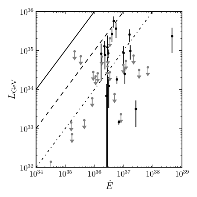
Figure 9.1: The observed $\gamma$-ray luminosities plotted against the observed spin-down luminosities for the PWNe candidates from Table 9.1.

In Figure 9.1, we compare the observed luminosity at GeV energies to the spin-down power of the observed pulsar. This plot shows that all LAT-detected PWNe emit a fraction $\lesssim 10\%$ of their spin-down energy into the $\gamma$-ray emission from the PWN.

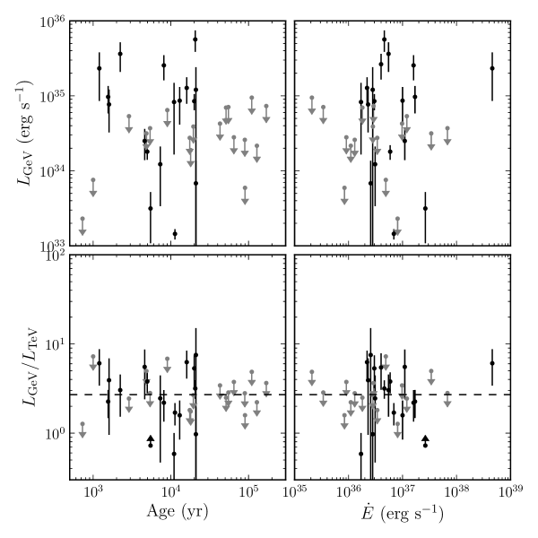
Figure 9.2: The observed $\gamma$-ray luminosities and the GeV to TeV luminosity ratios as a function of the ages and spin-down energies for the PWN candidates from Table 9.1. The dotted line corresponds to the average luminosity ratio ($\bar{R}$). Because 1708 1825HESS J1825$-$137 1640HESS J1640$-$465 1837HESS J1837$-$069 1632HESS J1632$-$478 1614HESS J1614$-$518 1616HESS J1616$-$508 1119HESS J1119$-$614 1303HESS J1303$-$631 1420HESS J1420$-$607 1841HESS J1841$-$055 1356HESS J1356$-$645 1023HESS J1023$-$575 1848HESS J1848$-$018 1514HESS J1514$-$591 1857HESS J1857$+$026 1708HESS J1708$-$443 1804HESS J1804$-$216 1634HESS J1634$-$472 1018HESS J1018$-$589 1507HESS J1507$-$622 1834HESS J1834$-$087 [] is classified as being a “PSR”-type source in Chapter 8, we consider the observed $\gamma$-ray luminosity of it to be an upper limit on the PWN emission. .

Next, in Figure 9.2 we compare compare the GeV luminosities and GeV to TeV luminosity ratios as a function of ages and spin-down energies of the host pulsars. These plots shows that there is no correlation between the GeV luminosities or GeV to TeV luminosity ratios and the ages and spin-down energies of the associate pulsars. In addition, we overlay the mean GeV to TeV luminosity ratio ($\bar{R}=2.7_{-1.4}^{+2.7}$).

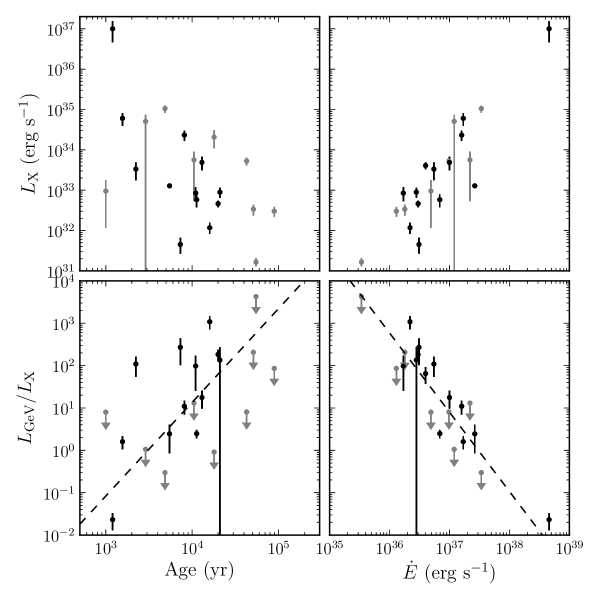
Figure 9.3: The observed X-ray flux and GeV to TeV luminosity ratios as a function of the age and spin-down energies for the PWN candidates from Table 9.1. The dotted line corresponds to the scaling relationships from Mattana et al. (2009) for the TeV to X-ray luminosity ratio scaled by the average GeV to TeV luminosity ($\bar{R}$). We caution that 3C 58 does not have a X-ray luminosity error.

Finally, in Figure 9.3 we compare the distribution of the X-ray luminosities and the GeV to X-ray luminosity ratios as a function of the ages and spin-down energies of the pulsars. This plot shows that the X-ray luminosity decreases with pulsar age and increases with spin-down energy. Similarly, the GeV to X-ray luminosity increases with age and decreases with energy. These correlations are consistent with the simple model predicted in Mattana et al. (2009) (See Section 3.5) and also with the observed VHE relationships from the same paper.

Chapter 10 Outlook

Since the observation of the Crab Nebula in 1989 (Weekes et al. 1989), we have learned much about the high-energy IC emission from PWN. The current generation of VHE experiments (H.E.S.S., Magic, and Veritas) have drastically expanded the population of PWN observed at $\gamma$-ray energies and PWNe are the most populous class of VHE sources in the Galaxy. Now, using the LAT on board Fermi, we have detected a large fraction of these VHE PWN at GeV energies and one PWN not yet detected at VHE energies.

The next great improvement in our knowledge of PWN will most likely come from next-generation IACTs. The proposed the Cherenkov Telescope Array (CTA) (Actis et al. 2011) will have a much improved effective area and angular resolution, allowing for the discovery of more VHE PWN as well as improved imaging of PWN candidates.

As was the case for 1825 1825HESS J1825$-$137 1640HESS J1640$-$465 1837HESS J1837$-$069 1632HESS J1632$-$478 1614HESS J1614$-$518 1616HESS J1616$-$508 1119HESS J1119$-$614 1303HESS J1303$-$631 1420HESS J1420$-$607 1841HESS J1841$-$055 1356HESS J1356$-$645 1023HESS J1023$-$575 1848HESS J1848$-$018 1514HESS J1514$-$591 1857HESS J1857$+$026 1708HESS J1708$-$443 1804HESS J1804$-$216 1634HESS J1634$-$472 1018HESS J1018$-$589 1507HESS J1507$-$622 1834HESS J1834$-$087 [], energy-dependent morphology at VHE energies can be used to unambiguous identify VHE emission as being caused by a pulsar (Aharonian et al. 2006c). Similarly, Van Etten & Romani (2011) showed for 1825 1825HESS J1825$-$137 1640HESS J1640$-$465 1837HESS J1837$-$069 1632HESS J1632$-$478 1614HESS J1614$-$518 1616HESS J1616$-$508 1119HESS J1119$-$614 1303HESS J1303$-$631 1420HESS J1420$-$607 1841HESS J1841$-$055 1356HESS J1356$-$645 1023HESS J1023$-$575 1848HESS J1848$-$018 1514HESS J1514$-$591 1857HESS J1857$+$026 1708HESS J1708$-$443 1804HESS J1804$-$216 1634HESS J1634$-$472 1018HESS J1018$-$589 1507HESS J1507$-$622 1834HESS J1834$-$087 [] that detailed spatial and spectral observations combined with multi-zone modeling can constrain the properties of the PWN. Detailed energy-dependent imaging of a larger sample of PWN by CTA will allow us a greater understanding of the physics of pulsar winds.

In addition, the Crab nebula has challenged our basic understand of the physics of PWNe. It is possible that more detailed observations could uncover additional variable PWN and this could help to explain the nature of this variable emission.

Finally, because of the high density of VHE PWN in the galactic plane, it is important to identify VHE sources as PWN to assist in the search for new source classes. There is significant potential for the discovery of new VHE source classes, but only after the numerous VHE PWN are classified. If the past is any guide to the future, there is much still to be learned.

References

- Abdo et al. (2010) Abdo, A., Ackermann, M., Ajello, M., et al. 2010, Astrophys.J., 722, 1303
- Abdo et al. (in prep) Abdo, A. A., Ajello, M., Allafort, A., Baldini, L., & et al. in prep, ApJS
- Abdo et al. (2007) Abdo, A. A., Allen, B., Berley, D., et al. 2007, ApJ, 664, L91
- Abdo et al. (2009a) Abdo, A. A., Ackermann, M., Ajello, M., et al. 2009a, ApJ, 699, L102
- Abdo et al. (2009b) —. 2009b, Physical Review Letters, 103, 251101
- Abdo et al. (2009c) Abdo, A. A., Ackermann, M., Atwood, W. B., et al. 2009c, ApJ, 696, 1084
- Abdo et al. (2009d) Abdo, A. A., Ackermann, M., Ajello, M., et al. 2009d, ApJ, 706, L1
- Abdo et al. (2009e) —. 2009e, ApJS, 183, 46
- Abdo et al. (2009f) Abdo, A. A., Allen, B. T., Aune, T., et al. 2009f, ApJ, 700, L127
- Abdo et al. (2009g) Abdo, A. A., Ackermann, M., Ajello, M., et al. 2009g, Astroparticle Physics, 32, 193
- Abdo et al. (2010a) —. 2010a, ApJ, 714, 927
- Abdo et al. (2010b) Abdo, A. A., Ackermann, M., Ajello, M., et al. 2010b, A&A, 523, A46
- Abdo et al. (2010c) Abdo, A. A., Ackermann, M., Ajello, M., et al. 2010c, Science, 328, 725
- Abdo et al. (2010d) —. 2010d, ApJS, 188, 405
- Abdo et al. (2010e) —. 2010e, ApJ, 708, 1254
- Abdo et al. (2010f) —. 2010f, ApJ, 718, 348
- Abdo et al. (2010) Abdo, A. A., Ackermann, M., Ajello, M., et al. 2010, The Astrophysical Journal, 713, 146
- Abdo et al. (2010a) Abdo, A. A., Ackermann, M., Ajello, M., et al. 2010a, Science, 327, 1103
- Abdo et al. (2010b) —. 2010b, ApJ, 712, 459
- Abdo et al. (2010c) Abdo, A. A., Ackermann, M., Ajello, M., et al. 2010c, A&A, 512, A7
- Abdo et al. (2010d) Abdo, A. A., Ackermann, M., Ajello, M., et al. 2010d, Physical Review Letters, 104, 101101
- Abdo et al. (2010e) —. 2010e, ApJS, 187, 460
- Abdo et al. (2011a) —. 2011a, Science, 331, 739
- Abdo et al. (2011b) —. 2011b, ApJ, 734, 28
- Abdo et al. (2012) Abdo, A. A., Wood, K. S., DeCesar, M. E., et al. 2012, ApJ, 744, 146
- Acciari et al. (2009) Acciari, V. A., Aliu, E., Arlen, T., et al. 2009, ApJ, 698, L133
- Acciari et al. (2010) —. 2010, ApJ, 719, L69
- Acciari et al. (2011) —. 2011, ApJ, 738, 3
- Acero et al. (in prep.) Acero, F., Ackermann, M., Ajello, M., & et al. in prep., ApJ
- Acero et al. (2012) Acero, F., Djannati-Ataï, A., Förster, A., et al. 2012, ArXiv e-prints
- Ackermann et al. (in prep) Ackermann, M., Ajello, M., Allafort, A., et al. in prep, ApJ
- Ackermann et al. (2011a) Ackermann, M., Ajello, M., Baldini, L., et al. 2011a, ApJ, 726, 35
- Ackermann et al. (2011b) Ackermann, M., Ajello, M., Allafort, A., et al. 2011b, ApJ, 743, 171
- Ackermann et al. (2012) Ackermann, M., Ajello, M., Atwood, W. B., et al. 2012, The Astrophysical Journal, 750, 3
- Ackermann et al. (2012) Ackermann, M., Ajello, M., Albert, A., et al. 2012, ApJS, 203, 4
- Actis et al. (2011) Actis, M., Agnetta, G., Aharonian, F., et al. 2011, Experimental Astronomy, 32, 193
- Aharonian et al. (2005a) Aharonian, F., Akhperjanian, A. G., Aye, K.-M., et al. 2005a, A&A, 435, L17
- Aharonian et al. (2005b) —. 2005b, A&A, 439, 1013
- Aharonian et al. (2006a) Aharonian, F., Akhperjanian, A. G., Bazer-Bachi, A. R., et al. 2006a, A&A, 460, 743
- Aharonian et al. (2006b) —. 2006b, A&A, 456, 245
- Aharonian et al. (2006c) —. 2006c, A&A, 460, 365
- Aharonian et al. (2006d) —. 2006d, A&A, 448, L43
- Aharonian et al. (2006e) —. 2006e, ApJ, 636, 777
- Aharonian et al. (2007a) —. 2007a, A&A, 467, 1075
- Aharonian et al. (2007b) —. 2007b, A&A, 472, 489
- Aharonian et al. (2007c) —. 2007c, ApJ, 661, 236
- Aharonian et al. (2007d) —. 2007d, A&A, 464, 235
- Aharonian et al. (2008a) —. 2008a, A&A, 481, 401
- Aharonian et al. (2008b) Aharonian, F., Akhperjanian, A. G., Barres de Almeida, U., et al. 2008b, A&A, 484, 435
- Aharonian et al. (2008c) —. 2008c, A&A, 477, 353
- Aharonian et al. (2009) Aharonian, F., Akhperjanian, A. G., Anton, G., et al. 2009, A&A, 499, 723
- Aharonian & Bogovalov (2003) Aharonian, F. A., & Bogovalov, S. V. 2003, New A, 8, 85
- Aharonian et al. (1994) Aharonian, F. A., Coppi, P. S., & Voelk, H. J. 1994, ApJ, 423, L5
- Aharonian et al. (2005c) Aharonian, F. A., Akhperjanian, A. G., Bazer-Bachi, A. R., et al. 2005c, A&A, 442, L25
- Aharonian et al. (2007e) —. 2007e, A&A, 469, L1
- Ajello et al. (2012) Ajello, M., Allafort, A., Baldini, L., et al. 2012, ApJ, 744, 80
- Akaike (1974) Akaike, H. 1974, IEEE Transactions on Automatic Control, 19, 716
- Albert et al. (2006) Albert, J., Aliu, E., Anderhub, H., et al. 2006, Science, 312, 1771
- Aliu (2011) Aliu, E. 2011, in International Cosmic Ray Conference, Vol. 7, International Cosmic Ray Conference, 227
- Arnold et al. (1962) Arnold, J. R., Metzger, A. E., Anderson, E. C., & van Dilla, M. A. 1962, J. Geophys. Res., 67, 4878
- Arons (1996) Arons, J. 1996, Space Sci. Rev., 75, 235
- Ashworth (1981) Ashworth, William B., J. 1981, Proceedings of the American Philosophical Society, 125, pp. 52
- Atwood et al. (2009) Atwood, W. B., Abdo, A. A., Ackermann, M., et al. 2009, ApJ, 697, 1071
- Baade & Zwicky (1934) Baade, W., & Zwicky, F. 1934, Physical Review, 46, 76
- Balbo et al. (2010) Balbo, M., Saouter, P., Walter, R., et al. 2010, A&A, 520, A111
- Baltz et al. (2008) Baltz, E. A., Berenji, B., Bertone, G., et al. 2008, J. Cosmology Astropart. Phys, 7, 13
- Bamba et al. (2003) Bamba, A., Ueno, M., Koyama, K., & Yamauchi, S. 2003, The Astrophysical Journal, 589, 253
- Bartoli et al. (2012) Bartoli, B., Bernardini, P., Bi, X. J., et al. 2012, ApJ, 745, L22
- Baum et al. (1946) Baum, W. A., Johnson, F. S., Oberly, J. J., et al. 1946, Phys. Rev., 70, 781
- Bertsch et al. (1992) Bertsch, D. L., Brazier, K. T. S., Fichtel, C. E., et al. 1992, Nature, 357, 306
- Bignami et al. (1975) Bignami, G. F., Boella, G., Burger, J. J., et al. 1975, Space Science Instrumentation, 1, 245
- Blandford & Romani (1988) Blandford, R. D., & Romani, R. W. 1988, MNRAS, 234, 57P
- Blumenthal & Gould (1970) Blumenthal, G. R., & Gould, R. J. 1970, Rev. Mod. Phys., 42, 237
- Bogovalov & Aharonian (2000) Bogovalov, S. V., & Aharonian, F. A. 2000, MNRAS, 313, 504
- Bolton et al. (1949) Bolton, J. G., Stanley, G. J., & Slee, O. B. 1949, Nature, 164, 101
- Bowyer et al. (1964) Bowyer, S., Byram, E. T., Chubb, T. A., & Friedman, H. 1964, Science, 146, 912
- Bradt et al. (1969) Bradt, H., Rappaport, S., & Mayer, W. 1969, Nature, 222, 728
- Browning et al. (1971) Browning, R., Ramsden, D., & Wright, P. J. 1971, Nature Physical Science, 232, 99
- Brumfiel (2007) Brumfiel, G. 2007, Nature, 448, 974
- Buehler et al. (2012) Buehler, R., Scargle, J. D., Blandford, R. D., et al. 2012, ApJ, 749, 26
- Burnham & Anderson (2002) Burnham, K. P., & Anderson, D. R. 2002, Model selection and multimodel inference: a practical information-theoretic approach, 2nd edn. (Springer)
- Burnight (1949) Burnight, T. 1949, Phys. Rev, 76, 19
- Caballero & Wilms (2012) Caballero, I., & Wilms, J. 2012, Mem. Soc. Astron. Italiana, 83, 230
- Carroll & Ostlie (2006) Carroll, B. W., & Ostlie, D. A. 2006, An Introduction to Modern Astrophysics, 2nd edn. (Benjamin Cummings)
- Cash (1979) Cash, W. 1979, ApJ, 228, 939
- Castelletti et al. (2006) Castelletti, G., Dubner, G., Golap, K., & Goss, W. M. 2006, A&A, 459, 535
- Caswell et al. (1981) Caswell, J. L., Milne, D. K., & Wellington, K. J. 1981, MNRAS, 195, 89
- Chandrasekhar (1931) Chandrasekhar, S. 1931, ApJ, 74, 81
- Chaves et al. (2008) Chaves, R. C. G., Renaud, M., Lemoine-Goumard, M., & Goret, P. 2008, in American Institute of Physics Conference Series, Vol. 1085, American Institute of Physics Conference Series, ed. F. A. Aharonian, W. Hofmann, & F. Rieger, 372–375
- Chen et al. (2011) Chen, A. W., Piano, G., Tavani, M., et al. 2011, A&A, 525, A33
- Cheng et al. (1986) Cheng, K. S., Ho, C., & Ruderman, M. 1986, ApJ, 300, 522
- Clifton et al. (1992) Clifton, T. R., Lyne, A. G., Jones, A. W., McKenna, J., & Ashworth, M. 1992, MNRAS, 254, 177
- Cocke et al. (1969) Cocke, W. J., Disney, M. J., & Taylor, D. J. 1969, Nature, 221, 525
- Collins et al. (1999) Collins, II, G. W., Claspy, W. P., & Martin, J. C. 1999, PASP, 111, 871
- Dame (2011) Dame, T. M. 2011, ArXiv e-prints
- Daugherty & Harding (1996) Daugherty, J. K., & Harding, A. K. 1996, ApJ, 458, 278
- de Geus et al. (1990) de Geus, E. J., Bronfman, L., & Thaddeus, P. 1990, A&A, 231, 137
- de Jager & Djannati-Ataï (2009) de Jager, O. C., & Djannati-Ataï, A. 2009, in Astrophysics and Space Science Library, Vol. 357, Astrophysics and Space Science Library, ed. W. Becker, 451
- de los Reyes et al. (2012) de los Reyes, R., Zajczyk, A., Chaves, R. C. G., & for the H. E. S. S. collaboration. 2012, ArXiv e-prints
- de Naurois & H.E.S.S. Collaboration (2013) de Naurois, M., & H.E.S.S. Collaboration. 2013, Advances in Space Research, 51, 258
- de Palma et al. (2013) de Palma, F., Brandt, T. J., Johannesson, G., Tibaldo, L., & for the Fermi LAT collaboration. 2013, in Fourth International Fermi Symposium
- Demorest et al. (2010) Demorest, P. B., Pennucci, T., Ransom, S. M., Roberts, M. S. E., & Hessels, J. W. T. 2010, Nature, 467, 1081
- Djannati-Ataĭ et al. (2008) Djannati-Ataĭ, A., de Jager, O. C., Terrier, R., & et al. 2008, in International Cosmic Ray Conference, Vol. 2, International Cosmic Ray Conference, 823–826
- Domainko & Ohm (2012) Domainko, W., & Ohm, S. 2012, A&A, 545, A94
- Dombrovsky (1954) Dombrovsky, V. A. 1954, Doklady Akademiya Nauk USSR, 94, 1021
- Drury et al. (1994) Drury, L. O., Aharonian, F. A., & Voelk, H. J. 1994, A&A, 287, 959
- Duncan (1921) Duncan, J. C. 1921, Proceedings of the National Academy of Science, 7, 179
- Dyks & Rudak (2003) Dyks, J., & Rudak, B. 2003, ApJ, 598, 1201
- Eadie et al. (1971) Eadie, W. T., Drijard, D., & James, F. E. 1971, Statistical methods in experimental physics (North-Holland Pub. Co.)
- Espinoza et al. (2011) Espinoza, C. M., Lyne, A. G., Kramer, M., Manchester, R. N., & Kaspi, V. M. 2011, ApJ, 741, L13
- Falanga et al. (2005) Falanga, M., Kuiper, L., Poutanen, J., et al. 2005, A&A, 444, 15
- Feenberg & Primakoff (1948) Feenberg, E., & Primakoff, H. 1948, Phys. Rev., 73, 449
- Fichtel et al. (1975) Fichtel, C. E., Hartman, R. C., Kniffen, D. A., et al. 1975, ApJ, 198, 163
- Finley et al. (1996) Finley, J. P., Srinivasan, R., & Park, S. 1996, ApJ, 466, 938
- Fisher (1925) Fisher, R. A. 1925, Statistical Methods for Research Workers (Edinburgh: Oliver and Boyd)
- Fritz et al. (1969) Fritz, G., Henry, R. C., Meekins, J. F., Chubb, T. A., & Friedman, H. 1969, Science, 164, 709
- Funk et al. (2007) Funk, S., Hinton, J. A., Pühlhofer, G., et al. 2007, ApJ, 662, 517
- Gaensler et al. (2003) Gaensler, B. M., Schulz, N. S., Kaspi, V. M., Pivovaroff, M. J., & Becker, W. E. 2003, ApJ, 588, 441
- Gaensler & Slane (2006) Gaensler, B. M., & Slane, P. O. 2006, ARA&A, 44, 17
- Gaisser et al. (1998) Gaisser, T. K., Protheroe, R. J., & Stanev, T. 1998, ApJ, 492, 219
- Gelfand et al. (2009) Gelfand, J. D., Slane, P. O., & Zhang, W. 2009, ApJ, 703, 2051
- Giordano & Fermi LAT Collaboration (2011) Giordano, F., & Fermi LAT Collaboration. 2011, in High-Energy Emission from Pulsars and their Systems, ed. D. F. Torres & N. Rea, 69
- Gold (1968) Gold, T. 1968, Nature, 218, 731
- Goldreich & Julian (1969) Goldreich, P., & Julian, W. H. 1969, ApJ, 157, 869
- Górski et al. (2005) Górski, K. M., Hivon, E., Banday, A. J., et al. 2005, ApJ, 622, 759
- Gotthelf & Halpern (2008) Gotthelf, E. V., & Halpern, J. P. 2008, ApJ, 681, 515
- Gould & Burbidge (1965) Gould, R. J., & Burbidge, G. R. 1965, Annales d’Astrophysique, 28, 171
- Grenier et al. (2005) Grenier, I. A., Casandjian, J.-M., & Terrier, R. 2005, Science, 307, 1292
- Grindlay & Hoffman (1971) Grindlay, J. E., & Hoffman, J. A. 1971, Astrophys. Lett., 8, 209
- Grondin et al. (2013) Grondin, M.-H., Romani, R. W., Lemoine-Goumard, M., et al. 2013
- Grondin et al. (2011) Grondin, M.-H., Funk, S., Lemoine-Goumard, M., et al. 2011, ApJ, 738, 42
- Gunn & Ostriker (1969) Gunn, J. E., & Ostriker, J. P. 1969, Nature, 221, 454
- H. E. S. S. Collaboration et al. (2012) H. E. S. S. Collaboration, Abramowski, A., Acero, F., et al. 2012, A&A, 541, A5
- Hall et al. (2003) Hall, T. A., Bond, I. H., Bradbury, S. M., et al. 2003, ApJ, 583, 853
- Hartman et al. (1999) Hartman, R. C., Bertsch, D. L., Bloom, S. D., et al. 1999, ApJS, 123, 79
- Haug (1975) Haug, E. 1975, Zeitschrift Naturforschung Teil A, 30, 1099
- Haug (1997) —. 1997, A&A, 326, 417
- Hayakawa (1952) Hayakawa, S. 1952, Progress of Theoretical Physics, 8, 571
- Heitler (1954) Heitler, W. 1954, The Quantum Theory of Radiation, Dover Books on Physics Series (New York : Dover Publications, Incorporated)
- Herschel (1800) Herschel, W. 1800, Philosophical Transactions of the Royal Society of London, 90, pp. 284
- H.E.S.S. Collaboration et al. (2011a) H.E.S.S. Collaboration, Abramowski, A., Acero, F., et al. 2011a, A&A, 531, A81
- H.E.S.S. Collaboration et al. (2011b) —. 2011b, A&A, 528, A143
- H.E.S.S. Collaboration et al. (2011c) H.E.S.S. Collaboration, Acero, F., Aharonian, F., et al. 2011c, A&A, 525, A45
- H.E.S.S. Collaboration et al. (2011d) H.E.S.S. Collaboration, Abramowski, A., Acero, F., et al. 2011d, A&A, 533, A103
- H.E.S.S. Collaboration et al. (2011e) —. 2011e, A&A, 525, A46
- Hessels et al. (2008) Hessels, J. W. T., Nice, D. J., Gaensler, B. M., et al. 2008, ApJ, 682, L41
- Hester (2008) Hester, J. J. 2008, ARA&A, 46, 127
- Hewish et al. (1968) Hewish, A., Bell, S. J., Pilkington, J. D. H., Scott, P. F., & Collins, R. A. 1968, Nature, 217, 709
- Hewitt et al. (2012) Hewitt, J., Grondin, M.-H., Lemoine-Goumard, M., et al. 2012
- Hofverberg (2011) Hofverberg, P. 2011, in International Cosmic Ray Conference, Vol. 7, International Cosmic Ray Conference, 247
- Hoppe (2008) Hoppe, S. 2008, in International Cosmic Ray Conference, Vol. 2, International Cosmic Ray Conference, 579–582
- Houck & Allen (2006) Houck, J. C., & Allen, G. E. 2006, ApJS, 167, 26
- Hutchinson (1952) Hutchinson, G. 1952, Philosophical Magazine Series 7, 43, 847
- Hwang et al. (2008) Hwang, U., Petre, R., & Flanagan, K. A. 2008, ApJ, 676, 378
- Jackson et al. (2005) Jackson, B., Scargle, J. D., Barnes, D., et al. 2005, IEEE Signal Processing Letters, 12, 105
- James & Roos (1975) James, F., & Roos, M. 1975, Computer Physics Communications, 10, 343
- Jansky (1933) Jansky, K. 1933, Proceedings of the Institute of Radio Engineers, 21, 1387
- Kamae et al. (2006) Kamae, T., Karlsson, N., Mizuno, T., Abe, T., & Koi, T. 2006, ApJ, 647, 692
- Kargaltsev et al. (2008) Kargaltsev, O., Pavlov, G. G., & Wong, J. A. 2008, ArXiv e-prints
- Kaspi & Helfand (2002) Kaspi, V. M., & Helfand, D. J. 2002, in Astronomical Society of the Pacific Conference Series, Vol. 271, Neutron Stars in Supernova Remnants, ed. P. O. Slane & B. M. Gaensler, 3
- Kaspi et al. (2006) Kaspi, V. M., Roberts, M. S. E., & Harding, A. K. 2006, Isolated neutron stars, ed. W. H. G. Lewin & M. van der Klis, 279–339
- Katagiri et al. (2011) Katagiri, H., Tibaldo, L., Ballet, J., et al. 2011, ApJ, 741, 44
- Katsuta et al. (2012) Katsuta, J., Uchiyama, Y., Tanaka, T., et al. 2012
- Kennel & Coroniti (1984a) Kennel, C. F., & Coroniti, F. V. 1984a, ApJ, 283, 694
- Kennel & Coroniti (1984b) —. 1984b, ApJ, 283, 710
- Kerr (2010) Kerr, M. 2010, PhD thesis, University of Washington
- Kijak & Gil (2003) Kijak, J., & Gil, J. 2003, A&A, 397, 969
- King (1962) King, I. 1962, AJ, 67, 471
- Klein & Nishina (1929) Klein, O., & Nishina, T. 1929, Zeitschrift fur Physik, 52, 853
- Kniffen & Fichtel (1970) Kniffen, D. A., & Fichtel, C. E. 1970, ApJ, 161, L157
- Koch & Motz (1959) Koch, H. W., & Motz, J. W. 1959, Reviews of Modern Physics, 31, 920
- Konopelko (2008) Konopelko, A. 2008, in International Cosmic Ray Conference, Vol. 2, International Cosmic Ray Conference, 767–770
- Krause et al. (2011) Krause, J., Carmona, E., Reichardt, I., & for the MAGIC Collaboration. 2011, ArXiv e-prints
- Kraushaar et al. (1965) Kraushaar, W., Clark, G. W., Garmire, G., et al. 1965, ApJ, 141, 845
- Kraushaar et al. (1972) Kraushaar, W. L., Clark, G. W., Garmire, G. P., et al. 1972, ApJ, 177, 341
- Lampland (1921) Lampland, C. O. 1921, PASP, 33, 79
- Lande et al. (2012) Lande, J., Ackermann, M., Allafort, A., et al. 2012
- Landi et al. (2007a) Landi, R., de Rosa, A., Dean, A. J., et al. 2007a, MNRAS, 380, 926
- Landi et al. (2007b) Landi, R., Masetti, N., Bassani, L., et al. 2007b, The Astronomer’s Telegram, 1047, 1
- Large et al. (1968) Large, M. I., Vaughan, A. E., & Mills, B. Y. 1968, Nature, 220, 340
- Lemoine-Goumard et al. (2011a) Lemoine-Goumard, M., Ferrara, E., Grondin, M.-H., Martin, P., & Renaud, M. 2011a, Mem. Soc. Astron. Italiana, 82, 739
- Lemoine-Goumard et al. (2011b) Lemoine-Goumard, M., Zavlin, V. E., Grondin, M.-H., et al. 2011b, A&A, 533, A102
- Li & Ma (1983) Li, T.-P., & Ma, Y.-Q. 1983, ApJ, 272, 317
- Longair (2011) Longair, M. S. 2011, High Energy Astrophysics, 3rd edn. (The Edinburgh Building, Cambridge CB2 8RU, UK: Cambridge University Press)
- Lundmark (1921) Lundmark, K. 1921, PASP, 33, 225
- Manchester et al. (2005) Manchester, R. N., Hobbs, G. B., Teoh, A., & Hobbs, M. 2005, AJ, 129, 1993
- Markwardt & Ogelman (1995) Markwardt, C. B., & Ogelman, H. 1995, Nature, 375, 40
- Matsumoto et al. (2007) Matsumoto, H., Ueno, M., Bamba, A., et al. 2007, PASJ, 59, 199
- Matsumoto et al. (2008) Matsumoto, H., Uchiyama, H., Sawada, M., et al. 2008, PASJ, 60, 163
- Mattana et al. (2009) Mattana, F., Falanga, M., Götz, D., et al. 2009, ApJ, 694, 12
- Mattox et al. (1992) Mattox, J. R., Bertsch, D. L., Fichtel, C. E., et al. 1992, ApJ, 401, L23
- Mattox et al. (1996) Mattox, J. R., Bertsch, D. L., Chiang, J., et al. 1996, ApJ, 461, 396
- Mayall & Oort (1942) Mayall, N. U., & Oort, J. H. 1942, PASP, 54, 95
- Mayer-Hasselwander et al. (1982) Mayer-Hasselwander, H. A., Kanbach, G., Bennett, K., et al. 1982, A&A, 105, 164
- McArthur (2011) McArthur, S. 2011, ArXiv e-prints
- McK Mahille et al. (2007) McK Mahille, J., Schild, R., Wendorf, F., & Brenmer, R. 2007, African Skies, 11, 2
- Meegan et al. (2009) Meegan, C., Lichti, G., Bhat, P. N., et al. 2009, ApJ, 702, 791
- Mizukami et al. (2011) Mizukami, T., Kubo, H., Yoshida, T., et al. 2011, ApJ, 740, 78
- Morrison (1958) Morrison, P. 1958, Il Nuovo Cimento, 7, 858
- Moskalenko & Strong (2000) Moskalenko, I. V., & Strong, A. W. 2000, ApJ, 528, 357
- Murphy et al. (2007) Murphy, T., Mauch, T., Green, A., et al. 2007, MNRAS, 382, 382
- Muslimov & Harding (2004) Muslimov, A. G., & Harding, A. K. 2004, ApJ, 606, 1143
- Neronov et al. (2011) Neronov, A., Semikoz, D. V., Tinyakov, P. G., & Tkachev, I. I. 2011, A&A, 526, A90
- Nolan et al. (1993) Nolan, P. L., Arzoumanian, Z., Bertsch, D. L., et al. 1993, ApJ, 409, 697
- Nolan et al. (1996) Nolan, P. L., Fierro, J. M., Lin, Y. C., et al. 1996, A&AS, 120, C61
- Nolan et al. (2012) Nolan, P. L., Abdo, A. A., Ackermann, M., et al. 2012, ApJS, 199, 31
- O’Brien et al. (2008) O’Brien, J. T., Johnston, S., Kramer, M., et al. 2008, MNRAS, 388, L1
- Pacini (1967) Pacini, F. 1967, Nature, 216, 567
- Pacini (1968) —. 1968, Nature, 219, 145
- Pacini & Salvati (1973) Pacini, F., & Salvati, M. 1973, ApJ, 186, 249
- Parent et al. (2011) Parent, D., Kerr, M., den Hartog, P. R., et al. 2011, ApJ, 743, 170
- Paron et al. (2008) Paron, S., Dubner, G., Reynoso, E., & Rubio, M. 2008, A&A, 480, 439
- Pellizzoni et al. (2010) Pellizzoni, A., Trois, A., Tavani, M., et al. 2010, Science, 327, 663
- Petre et al. (1996) Petre, R., Becker, C. M., & Winkler, P. F. 1996, The Astrophysical Journal Letters, 465, L43
- Pittori & the AGILE Team (2003) Pittori, C., & the AGILE Team. 2003, Chinese Journal of Astronomy and Astrophysics, 3, 517
- Pollock (1985) Pollock, A. M. T. 1985, A&A, 150, 339
- Protassov et al. (2002) Protassov, R., van Dyk, D. A., Connors, A., Kashyap, V. L., & Siemiginowska, A. 2002, ApJ, 571, 545
- Rea & Esposito (2011) Rea, N., & Esposito, P. 2011, in High-Energy Emission from Pulsars and their Systems, ed. D. F. Torres & N. Rea, 247
- Rees & Gunn (1974) Rees, M. J., & Gunn, J. E. 1974, MNRAS, 167, 1
- Renaud et al. (2008) Renaud, M., Goret, P., & Chaves, R. C. G. 2008, in American Institute of Physics Conference Series, Vol. 1085, American Institute of Physics Conference Series, ed. F. A. Aharonian, W. Hofmann, & F. Rieger, 281–284
- Reynoso et al. (1995) Reynoso, E. M., Dubner, G. M., Goss, W. M., & Arnal, E. M. 1995, AJ, 110, 318
- Reynoso et al. (2003) Reynoso, E. M., Green, A. J., Johnston, S., et al. 2003, MNRAS, 345, 671
- Richards & Comella (1969) Richards, D. W., & Comella, J. M. 1969, Nature, 222, 551
- Rieke & Weekes (1969) Rieke, G. H., & Weekes, T. C. 1969, ApJ, 155, 429
- Rishbeth (1958) Rishbeth, H. 1958, Australian Journal of Physics, 11, 550
- Rodriguez et al. (2003) Rodriguez, J., Tomsick, J. A., Foschini, L., et al. 2003, A&A, 407, L41
- Romani (1996) Romani, R. W. 1996, ApJ, 470, 469
- Romani et al. (2011) Romani, R. W., Kerr, M., Craig, H. A., et al. 2011, ApJ, 738, 114
- Rousseau et al. (2012) Rousseau, R., Grondin, M.-H., Van Etten, A., et al. 2012, A&A, 544, A3
- Rowell et al. (2008) Rowell, G., Horns, D., Fukui, Y., & Moriguchi, Y. 2008, in American Institute of Physics Conference Series, Vol. 1085, American Institute of Physics Conference Series, ed. F. A. Aharonian, W. Hofmann, & F. Rieger, 241–244
- Rybicki & Lightman (1979) Rybicki, G. B., & Lightman, A. P. 1979, Radiative processes in astrophysics (New York: John Wiley & Sons Ltd)
- Scargle et al. (2013) Scargle, J. D., Norris, J. P., Jackson, B., & Chiang, J. 2013, ApJ, 764, 167
- Schwarz (1978) Schwarz, G. 1978, The Annals of Statistics, 6, pp. 461
- Seward & Harnden (1982) Seward, F. D., & Harnden, Jr., F. R. 1982, ApJ, 256, L45
- Shaver & Goss (1970) Shaver, P. A., & Goss, W. M. 1970, Australian Journal of Physics Astrophysical Supplement, 14, 133
- Sheidaei (2011) Sheidaei, F. 2011, in International Cosmic Ray Conference, Vol. 7, International Cosmic Ray Conference, 243
- Shklovskii (1953) Shklovskii, I. S. 1953, Doklady Akad. Nauk SSSR, 90, 983
- Slane et al. (2010) Slane, P., Castro, D., Funk, S., et al. 2010, The Astrophysical Journal, 720, 266
- Slane et al. (2010) Slane, P., Castro, D., Funk, S., et al. 2010, ApJ, 720, 266
- Slane et al. (2008) Slane, P., Helfand, D. J., Reynolds, S. P., et al. 2008, ApJ, 676, L33
- Slane et al. (2004) Slane, P., Helfand, D. J., van der Swaluw, E., & Murray, S. S. 2004, ApJ, 616, 403
- Sreekumar et al. (1999) Sreekumar, P., Bertsch, D. L., Hartman, R. C., Nolan, P. L., & Thompson, D. J. 1999, Astroparticle Physics, 11, 221
- Sreekumar et al. (1992) Sreekumar, P., Bertsch, D. L., Dingus, B. L., et al. 1992, ApJ, 400, L67
- Sreekumar et al. (1998) Sreekumar, P., Bertsch, D. L., Dingus, B. L., et al. 1998, The Astrophysical Journal, 494, 523
- Staelin & Reifenstein (1968) Staelin, D. H., & Reifenstein, III, E. C. 1968, Science, 162, 1481
- Strong & Moskalenko (1998) Strong, A. W., & Moskalenko, I. V. 1998, ApJ, 509, 212
- Sugizaki et al. (2001) Sugizaki, M., Mitsuda, K., Kaneda, H., et al. 2001, ApJS, 134, 77
- Swanenburg et al. (1978) Swanenburg, B. N., Hermsen, W., Bennett, K., et al. 1978, Nature, 275, 298
- Swanenburg et al. (1981) Swanenburg, B. N., Bennett, K., Bignami, G. F., et al. 1981, ApJ, 243, L69
- Tam et al. (2010) Tam, P. H. T., Wagner, S. J., Tibolla, O., & Chaves, R. C. G. 2010, A&A, 518, A8
- Tanaka et al. (2011) Tanaka, T., Allafort, A., Ballet, J., et al. 2011, ApJ, 740, L51
- Taylor et al. (2003) Taylor, A. R., Gibson, S. J., Peracaula, M., et al. 2003, AJ, 125, 3145
- Terrier et al. (2008) Terrier, R., Mattana, F., Djannati-Atai, A., et al. 2008, in American Institute of Physics Conference Series, Vol. 1085, American Institute of Physics Conference Series, ed. F. A. Aharonian, W. Hofmann, & F. Rieger, 312–315
- The Fermi LAT Collaboration et al. (2012) The Fermi LAT Collaboration, Coe, M. J., Di Mille, F., et al. 2012, ArXiv e-prints
- Thompson (2008) Thompson, D. J. 2008, Reports on Progress in Physics, 71, 116901
- Thompson et al. (1977a) Thompson, D. J., Fichtel, C. E., Hartman, R. C., Kniffen, D. A., & Lamb, R. C. 1977a, ApJ, 213, 252
- Thompson et al. (1977b) Thompson, D. J., Fichtel, C. E., Kniffen, D. A., & Ogelman, H. B. 1977b, ApJ, 214, L17
- Thompson et al. (1993) Thompson, D. J., Bertsch, D. L., Fichtel, C. E., et al. 1993, ApJS, 86, 629
- Tomsick et al. (2003) Tomsick, J. A., Lingenfelter, R., Walter, R., et al. 2003, IAU Circ., 8076, 1
- Torii et al. (2000) Torii, K., Slane, P. O., Kinugasa, K., Hashimotodani, K., & Tsunemi, H. 2000, PASJ, 52, 875
- Torii et al. (1998) Torii, K., Kinugasa, K., Toneri, T., et al. 1998, ApJ, 494, L207
- Trussoni et al. (1996) Trussoni, E., Massaglia, S., Caucino, S., Brinkmann, W., & Aschenbach, B. 1996, A&A, 306, 581
- van der Swaluw & Wu (2001) van der Swaluw, E., & Wu, Y. 2001, ApJ, 555, L49
- Van Etten & Romani (2011) Van Etten, A., & Romani, R. W. 2011, ApJ, 742, 62
- Vladimirov et al. (2011) Vladimirov, A. E., Digel, S. W., Jóhannesson, G., et al. 2011, Computer Physics Communications, 182, 1156
- Watters & Romani (2011) Watters, K. P., & Romani, R. W. 2011, ApJ, 727, 123
- Weekes et al. (1989) Weekes, T. C., Cawley, M. F., Fegan, D. J., et al. 1989, ApJ, 342, 379
- Weinstein & for the VERITAS Collaboration (2009) Weinstein, A., & for the VERITAS Collaboration. 2009, ArXiv e-prints
- Wilks (1938) Wilks, S. S. 1938, Annals of Mathematical Statistics, 9, 60
- Young et al. (1986) Young, E. T., Lada, C. J., & Wilking, B. A. 1986, ApJ, 304, L45