Investigating the Physics and Environment of Lyman Limit Systems in Cosmological Simulations

Abstract

In this work, I investigate the properties of Lyman limit systems (LLSs) using state-of-the-art zoom-in cosmological galaxy formation simulations with on the fly radiative transfer, which includes both the cosmic UV background (UVB) and local stellar sources. I compare the simulation results to observations of the incidence frequency of LLSs and the HI column density distribution function over the redshift range $z=2-5$ and find good agreement. I explore the connection between LLSs and their host halos and find that LLSs reside in halos with a wide range of halo masses with a nearly constant covering fraction within a virial radius. Over the range $z=2-5$, I find that more than half of the LLSs reside in halos with $M<10^{10}h^{-1}M_{\odot}$, indicating that absorption line studies of LLSs can probe these low-mass galaxies which H₂-based star formation models predict to have very little star formation. I study the physical state of individual LLSs and test a simple model (Schaye 2001) which encapsulates many of their properties. I confirm that LLSs have a characteristic absorption length given by the Jeans length and that they are in photoionization equilibrium at low column densities. Finally, I investigate the self-shielding of LLSs to the UVB and explore how the non-sphericity of LLSs affects the photoionization rate at a given $N_{\rm HI}$. I find that at $z\approx 3$, LLSs have an optical depth of unity at a column density of $\sim 10^{18}{\rm cm}^{-2}$ and that this is the column density which characterizes the onset of self-shielding.

1 Introduction

Lyman limit systems are a special class of Ly$\alpha$ absorbers which span a range of column densities: $N_{{\rm HI}}=1.6\times 10^{17}{\rm cm}^{-2}-2\times 10^{20}{\rm cm}^{-2}$. The lower limit is defined by the column density which gives an optical depth of unity at the Lyman limit and the upper limit is defined by the transition to Damped Ly$\alpha$ (DLA) systems which are mostly neutral. They are primarily observed through quasar absorption lines although their absorption features have also been seen in the spectra of gamma-ray bursts. See Rauch (1998); Meiksin (2009) for reviews of Ly$\alpha$ absorbers and Wolfe, Gawiser & Prochaska (2005) for a review of DLAs.

Observations of LLSs and DLAs in the high-redshift universe provide a fertile ground for comparison with theoretical work. They give a unique window into the high-redshift universe since the quasar absorption line observations provide an area-weighted survey of these absorbers across a large range of redshifts which makes them especially simple to compare with simulations.

While the absorption line studies provide rich statistics of these systems when averaged over many lines of sight, it is difficult to deduce the environment in which individual absorbers reside. The main goal of this work is to understand the environment of LLSs, as well the physical mechanisms which control their properties. Many groups have studied the properties of LLSs in simulations of varying mass resolution and with many of the physical mechanisms which affect LLSs (Kohler & Gnedin, 2007; Altay et al., 2011; McQuinn, Oh & Faucher-Giguère, 2011; Fumagalli et al., 2011; Yajima, Choi & Nagamine, 2012; Rahmati et al., 2013a, b; Rahmati & Schaye, 2014). The simulations in this work have a relatively high mass resolution of $1.5\times 10^{5}{\rm h}^{-1}M_{\odot}$, allowing us to study lower mass halos, $M<10^{9}{\rm h}^{-1}M_{\odot}$, than has previously been achieved. This mass range is especially interesting since H₂-based star formation models indicate that these halos will not form stars (Gnedin & Kravtsov, 2010; Kuhlen, Madau & Krumholz, 2013) and hence they may only be detectable using absorption line studies.

In addition to studying the halos in which LLSs reside, I will use these simulations to study the self-shielding of LLSs to the UVB. LLSs are defined as having an optical depth greater than unity to radiation at the Lyman limit, i.e. $N_{{\rm HI}}=10^{17.2}{\rm cm}^{-2}$. The column density at which this self-shielding becomes effective is important since it controls the turnover of the HI column density distribution as was shown in Altay et al. (2011); McQuinn, Oh & Faucher-Giguère (2011); Rahmati et al. (2013a). In Section 7, I will show that due to the physical properties and anisotropic shielding of LLSs, as well as the spectrum of the UVB, a column density of $N_{{\rm HI}}\sim 10^{18}{\rm cm}^{-2}$ is needed to shield against the UVB with an optical depth of unity at $z\approx 3$.

This paper is arranged as follows. In Section 2, I discuss the simulations used in this paper. Next, I compare the simulation results to quasar absorption line observations of the high-redshift universe in Section 3 and find that the simulations qualitatively reproduce the features seen in observations. In Section 4, I explore the relation between LLSs and their host halos and find that LLSs reside in halos with a large range of masses but that there is a cutoff at low mass which is similar to the cutoff due to photoheating from the UVB. In Section 5, I investigate the physical mechanisms of individual LLSs and test a simple model for LLSs developed in Schaye (2001). In Section 6, I study the anisotropy of LLSs and how this affects their self-shielding properties. In Section 7, I discuss how the physical properties of LLSs and the spectral shape of the UVB affect the amount of self-shielding in these systems. In Section 8, I compare the results from this work to some recent works on LLSs. Finally, I conclude in Section 9.

2 Simulations

In this work, I have used the simulation described in Zemp et al. (2012), carried out using the Adaptive Refinement Tree (ART) code (Kravtsov, 1999; Kravtsov, Klypin & Hoffman, 2002; Rudd, Zentner & Kravtsov, 2008). The code has adaptive mesh refinement which gives a large dynamic range in spatial scale. These simulations follow five different Lagrangian regions, each of five virial radii around a system which evolves into a typical halo of an $L_{*}$ galaxy (${\rm M}\approx 10^{12}{\rm M}_{\odot}$) at $z=0$. These Lagrangian regions are embedded in a cube of size $25.6$ comoving $h^{-1}$ Mpc to model the tidal forces from surrounding structures. The outer region is coarsely resolved with a uniform $256^{3}$ grid. The dark matter mass resolution is $1.5\times 10^{5}h^{-1}{\rm M}_{\odot}$ in the high-resolution Lagrangian region and the baryonic mass resolution varies from $\sim 10^{3}{\rm M}_{\odot}$ to $\sim 10^{6}{\rm M}_{\odot}$ depending on cell size and density. The maximum spatial resolution is $195$ comoving $h^{-1}$pc. The cosmological parameters used are similar to the WMAP7 parameters: $\Omega_{M}=0.28$, $\Omega_{B}=0.046$, $\sigma_{8}=0.82$, $h=0.7$, and $n_{s}=0.96$.

These simulations include three-dimensional radiative transfer of UV radiation from the UVB as well as from stars formed in the simulation. This is done with the Optically Thin Variable Eddington Tensor (OTVET) approximation (Gnedin & Abel, 2001). The contribution from the UVB uses the model in Haardt & Madau (2001), while the contribution from local sources uses a Miller-Scalo IMF (Miller & Scalo, 1979) and the shape of the spectrum from local sources comes from Starburst99 modeling Leitherer et al. (1999) and is plotted in Figure 4 of Ricotti, Gnedin & Shull (2002). The OTVET method in this work follows the transfer of radiation at 4 frequencies: at the ${\rm HI}$, ${\rm HeI}$, and ${\rm HeII}$ ionization thresholds, as well as one to follow non-ionizing radiation at 1000 Å. The fidelity of this RT prescription was tested in Iliev et al. (2006, 2009) where it was found to work well except for some numerical diffusion of ionization fronts. The prescription has subsequently been improved and numerical diffusion has been almost completely eliminated Gnedin (2014). This detailed and faithful radiative transfer allows us to model the self-shielding of LLSs against the UVB. It is also important for understanding the effect of local sources on LLSs since they arise in close proximity to galaxies.

These simulations include a self-consistent, non-equilibrium chemical network of hydrogen and helium, including the effects of ionization from photoionization (corrected for dust-shielding), collisional ionization, and radiative recombination Gnedin & Kravtsov (2011). The chemical network also self-consistently models $H_{2}$, including the formation of molecular hydrogen in both primordial phase and on dust grains (see Gnedin & Kravtsov, 2011, for details). This physics includes the cooling and physical mechanisms needed to correctly model the gas in LLSs and allows for a realistic H₂-based star-formation model.

Finally, the simulations include thermal supernova feedback with an energy deposition of $2\times 10^{51}$ erg from Type Ia and Type II supernovae. This feedback prescription is known to be inefficient since the supernova energy is deposited in cells with high densities and relatively low temperatures which results in extremely efficient cooling. While efficient feedback has been shown to increase the cross-section of LLSs (e.g. Faucher-Giguère et al., 2015; Rahmati et al., 2015) examining the effect of realistic feedback is beyond the scope of this work. Note that since feedback also depends on the mass of the host galaxy, the inclusion of more efficient feedback would also likely affect the LLS cross-section versus halo mass which is explored below.

3 Column Density Distribution and Incidence of LLSs

Before delving into the properties of individual absorbers and their host halos, it is useful to test how well the simulations are modeling the properties of LLSs by comparing against observations. Two of the main statistics for LLSs measured by observers are the number of LLSs per absorption length (the incidence frequency) and the number of systems per unit absorption length per unit column density (the HI column density distribution). The incidence frequency is written as,

$$l_{\rm LLS}=\frac{{\rm d}\mathcal{N}}{{\rm d}X},$$ (1)

and the HI column density distribution is written as,

$$f(N_{{\rm HI}},z)=\frac{{\rm d}^{2}\mathcal{N}}{{\rm d}N_{{\rm HI}}{\rm d}X},$$ (2)

where the absorption length is given by

$$\frac{{\rm d}X}{{\rm d}z}=\frac{H_{0}}{H(z)}(1+z)^{2}.$$ (3)

These statistics are related since the HI column density distribution is the incidence frequency per unit column density. The absorption length is defined this way so that absorbers with a constant comoving number density and constant physical size have a constant incidence frequency. Hence, any evolution in these quantities is due to evolution in the cross-section of these systems, their number density, or a combination of these two. Since LLSs reside in and around galaxies, their incidence can be written in terms of the average LLS cross-section, $\sigma_{\rm LLS}(M,z)$, and the halo mass function, $n(M,z)$, at redshift $z$ (Gardner et al., 1997):

$$l_{\rm LLS}=\frac{c}{H_{0}}\int{\sigma}_{\rm LLS}(M,z)n(M,z){\rm d}M.$$ (4)

Note that I will also consider the quantity $l_{\tau>\tau_{0}}$, which is the incidence of systems with an optical depth greater than $\tau_{0}$ at the Lyman limit. Likewise, the HI column density distribution can be written as

$$f(N_{{\rm HI}},z)=\frac{c}{H_{0}}\int\frac{\partial\sigma(N_{{\rm HI}},M,z)}{\partial N_{{\rm HI}}}n(M,z){\rm d}M,$$ (5)

where $\sigma(N_{{\rm HI}},M,z)$ is the average cross-section of absorbers with a column density below $N_{{\rm HI}}$ around halos of mass $M$.

3.1 Observations of LLSs

Observations of LLSs in the high-redshift universe are primarily made by using quasar absorption lines. Since LLSs correspond to the flat portion of the curve of growth, their column density is harder to determine than systems with lower or higher column densities. The column densities of systems in the Ly$\alpha$ forest with $N_{{\rm HI}}<10^{17.2}{\rm cm}^{-2}$ can be directly determined either from Voigt profile fits to the Ly$\alpha$ absorption, or from fits to higher order Lyman transitions (e.g. Rudie et al., 2012). For DLAs and sub-DLAs, $N_{{\rm HI}}>10^{19}{\rm cm}^{-2}$, the natural line width of the Ly$\alpha$ transition produces damping wings which make the column densities of these systems easy to determine (e.g. Wolfe, Gawiser & Prochaska, 2005). However, in the intermediate range, $10^{17.2}{\rm cm}^{-2}<N_{{\rm HI}}<10^{19}{\rm cm}^{-2}$, the exact column density is difficult to measure and requires precise observations of both the Ly$\alpha$ line and the Lyman limit break (e.g. Prochter et al., 2010). While the exact column density may be difficult to determine in this range, the presence of an absorber with $N_{{\rm HI}}>10^{17.2}{\rm cm}^{-2}$ can be inferred from the Lyman limit break. As a result, observers can more easily measure the number of systems above a given threshold (typically $N_{{\rm HI}}=10^{17.2}{\rm cm}^{-2}$) which provides an integral constraint on the HI column density distribution. In some works (i.e. O’Meara et al., 2013), this counting is done for multiple thresholds which can be used to constrain the column density distribution.

In Figure 1, I show observations of the incidence of LLSs over a variety of redshifts. These come from Prochaska, O’Meara & Worseck (2010) and O’Meara et al. (2013). In Figure 2, I show the constraints on the HI column density distribution for LLSs at $z\approx 2.4$ from O’Meara et al. (2007) and O’Meara et al. (2013). Above $N_{{\rm HI}}=10^{19}{\rm cm}^{-2}$ these constraints come from the detection of individual LLSs for which the HI column density of each system can be determined. Between $N_{{\rm HI}}=10^{17.5}{\rm cm}^{-2}$ and $N_{{\rm HI}}=10^{19}{\rm cm}^{-2}$, the constraints are determined from $l_{\tau>2}$. Below $N_{{\rm HI}}=10^{17.5}{\rm cm}^{-2}$, the constraints are determined from the comparison of $l_{\tau>2}$, $l_{\tau>1}$, and $l_{\tau>0.5}$ in O’Meara et al. (2013). See O’Meara et al. (2013) for a detailed discussion of these constraints.

3.2 Measuring the Frequency and Column Density Distribution in Simulations

Using a method similar to observations, the HI column density is computed by taking lines of sight through the simulation, measuring the HI column density along these lines of sight, and counting the number of absorbers in each column density bin. Observationally, the HI column densities are determined by fitting profiles to the HI absorption lines. In simulations, the HI column density can simply be integrated along lines of sight in the three cartesian directions. Since systems in the simulation are randomly oriented with respect to the simulation box, these lines of sight effectively probe random lines of sight through systems in the simulation. This method gives the same HI column density as fitting absorption lines as long as there are not multiple systems along each line of sight.

In order to determine the column density at which these projection effects become important, I considered lines of sight of various lengths along the cartesian directions. These lines of sight were placed on a regular grid separated by 4 times the highest resolution element, $781$ comoving $h^{-1}$ pc. This sampling fixes the number of lines of sight taken through the simulation volume but does not affect the resolution along the line of sight, which is controlled by the size of each cell. Along each line of sight, I found the location of the cell with the maximum HI density and defined this to be the center of the absorber. This definition will allow us to probe the environment which is physically close to the absorber since we can take lines of sight originating from this point. I then considered lines of sight of length 10kpc, 50kpc, 200kpc, and the full box length, centered on the absorber. I found that while the 10kpc and 50kpc lines of sight differed substantially below $N_{{\rm HI}}=10^{16}{\rm cm}^{-2}$, the 200kpc and full box lines of sight showed fairly similar column densities (only 2.5% of systems differed by more than a factor of 2) indicating that the projection effects are not substantial for these systems. In this work I will restrict the analysis to $N_{{\rm HI}}>10^{16.5}{\rm cm}^{-2}$ where projection effects are even less important. This approach was also taken in Altay et al. (2011) and Rahmati et al. (2013a) where the projected column density was used for systems with $N_{{\rm HI}}>10^{17}{\rm cm}^{-2}$ and $N_{{\rm HI}}>10^{16}{\rm cm}^{-2}$ respectively. Note that these shorter lines of sight target gas associated with the absorber and will also be used to measure quantities like the characteristic size of an absorber.

3.3 LLS Incidence Frequency

Due to the difficulty in directly measuring the column density of LLSs, the frequency of LLSs per unit absorption length is the natural quantity to compare against observations. I have computed this quantity using two approaches and plotted the result in Figure 1. First, I counted the number of LLSs above $N_{{\rm HI}}>10^{17.5}{\rm cm}^{-2}$ along all of the sightlines in the simulation, and then divided by the absorption length in the simulation:

$$l_{\rm\tau>2}=\frac{\Delta\mathcal{N}_{\tau>2}}{\Delta X}.$$ (6)

The result of this simple approach is shown in Figure 1 and is consistent with observations although it has a somewhat different evolution in redshift.

In the second approach, I attempted to account for the bias inherent in a zoom-in simulation by rescaling the contribution from each halo mass bin. Since the zoom-in regions are selected to have a Milky Way progenitor, the mass function in these regions will be biased as a random volume of this size would have fewer massive galaxies. One way to account for this is to identify each LLS with its host halo, compute the mean cross-section in each halo mass range, $\overline{\sigma}_{\tau>2}(M_{i},z)$, and then compute the quantity

$$l_{\tau>2}=\frac{c}{H_{0}}\sum_{i}\overline{\sigma}_{\tau>2}(M_{i},z)\overline{n}(M_{i},z),$$ (7)

where

$$\overline{n}(M_{i},z)=\int_{M_{i}}^{M_{i}+\Delta M}n(M,z){\rm d}M,$$ (8)

and $n(M,z)$ is the true halo mass function. As long as the cross-section of individual halos is correctly modeled, this discretized version of Equation (4) will partially correct for the bias of the zoom-in simulation. Note that I have restricted this sum to be over resolved halos with $M>10^{8}h^{-1}{\rm M}_{\odot}$ (corresponding to $\approx$1000 particles) below which we cannot model the cross-section and that I used the halo mass function from Sheth & Tormen (2002) as the true halo mass function. Also note that this sum is only covers the mass range of halos within the simulation but due to the rapidly falling halo mass function and the relatively constant LLS covering fraction which we will discuss in Section 4, the inclusion of higher mass halos should not significantly change this result. The corrected incidence frequency is plotted in Figure 1. It is lower than the basic counting result since it lowers the contribution from more massive halos. While the simulated incidence frequency is consistent with the observations until $z\sim 3.5$, there is significant deviation at higher redshift. This is likely due to the zoom-in simulations used in this work which cannot capture the contribution from the filamentary cosmic-web at high-redshifts. The mean cross-section computed in the simulation can be found in Figure 3 and will be discussed in more detail in Section 4.

This technique also relies on the properties of the galaxies in the zoom-in region being representative of the properties of average galaxies in the universe. While this bias cannot be addressed with individual zoom-in regions, simulations with fixed-resolution (i.e. Rahmati & Schaye, 2014) give similar results for the cumulative distribution function (CDF) of LLSs with respect to halo mass, indicating that the assumption is a reasonable one. In Figure 6 of Rahmati & Schaye (2014), the CDF shows a similar behavior to what is found in Figure 5 of this work with $\sim 75\%,\sim 15\%,$ and $\sim 10\%$ of LLSs arising in halos with masses in the range $M<10^{10}M_{\odot}$, $10^{10}M_{\odot}<M<10^{11}M_{\odot}$, and $M>10^{11}M_{\odot}$, respectively at $z=3$. In this work we find $\sim 71\%$, $\sim 22\%,$ and $\sim 7\%$ of LLSs arising in halos with the same mass range.

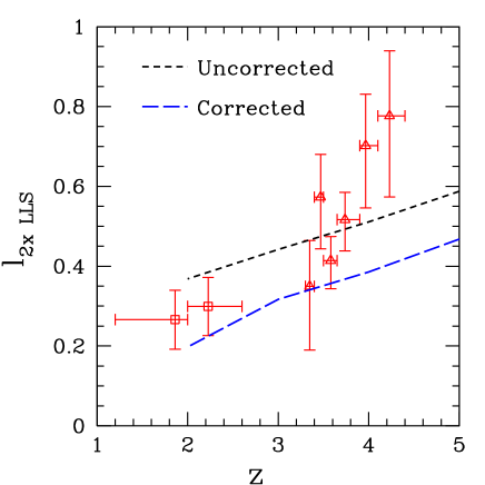
Figure 1: Incidence of systems with $N_{{\rm HI}}>10^{17.5}{\rm cm}^{-2}$ in simulations and observations as a function of redshift. The short-dashed black curve shows the basic estimate from counting the number of absorbers in the simulation and dividing by the absorption length of the simulation volume. The long-dashed blue curve shows the result of correcting for the halo mass function. The data are from two surveys: the squares are from O’Meara et al. (2013) and the triangles are from Prochaska, O’Meara & Worseck (2010).

3.4 Evolution of the HI Column Density Distribution

In order to compute the column density distribution, I count the number of absorbers in each HI column density bin, and divide by the total absorption length in the simulation:

$$f(N_{{\rm HI}})=\frac{\Delta\mathcal{N}(N_{{\rm HI}})}{\Delta N_{{\rm HI}}\Delta X}.$$ (9)

In Figure 2, I compare the HI column density distribution for LLSs in simulations to observations. Since the column density distribution is quite steep over this range, I have plotted the quantity $\log_{10}N_{{\rm HI}}f(N_{{\rm HI}},z)$ in order to aid comparison. The HI column density distribution in simulations has a qualitatively similar structure to the observed HI column density distribution. The column density distribution is steep at low $N_{{\rm HI}}$ and then flattens out when self-shielding becomes important as I will discuss further in Section 5. Once the gas becomes sufficiently neutral, the column density distribution steepens once again. This structure has been seen in many of the recent simulations of Ly$\alpha$ absorbers (i.e. McQuinn, Oh & Faucher-Giguère, 2011; Fumagalli et al., 2011; Altay et al., 2011; Rahmati et al., 2013a). In the observations, the flattening of the HI column density distribution is poorly constrained since it occurs on the flat portion of the curve of growth where there are only integral constraints on the HI column density distribution.

Interestingly, Figure 2 indicates that the HI column density distribution remains relatively flat over a larger range than seen in the observations. A similar shape was found in McQuinn, Oh & Faucher-Giguère (2011). Note that since the quantity being plotted is proportional to the number of absorbers per logarithmic $N_{{\rm HI}}$ bin, Figure 2 implies that there are more systems per logarithmic interval at $N_{{\rm HI}}=10^{20}{\rm cm}^{-2}$ than at $N_{{\rm HI}}=10^{19}{\rm cm}^{-2}$. A similar inversion is seen in the data although at slightly lower column density. I will discuss the location of this turnover further in Sec. 5.

From Figure 2, it is apparent that the shape of the HI column density distribution undergoes little evolution between $z=2$ and $z=5$, although there is a slight flattening at low column densities and low redshift. This lack of evolution agrees with the previous results found by Fumagalli et al. (2011) and Rahmati et al. (2013a). Note that this work finds slightly less evolution in the column density distribution from $z=5$ to $z=3$ than is found in Rahmati et al. (2013a). This difference is likely due to the same reason that I underpredict the incidence of LLS in Figure 1, the zoom-in simulations in this work do not capture the large-scale filaments at high redshift.

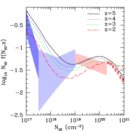
Figure 2: HI column density distribution compared to observations centered around $z\approx 2.4$. Since the column density distribution is fairly steep, I plot $\log_{10}N_{{\rm HI}}f(N_{{\rm HI}},z)$ so that the features are more salient. The light blue shaded region comes from constraints on $l_{\tau>2}$ from O’Meara et al. (2013). The dark blue shaded region comes from constraints on the slope of the column density distribution in the range $N_{{\rm HI}}\in 10^{16.9}-10^{17.5}{\rm cm}^{-2}$ from the constraints on $l_{\tau>2}$, $l_{\tau>1}$, and $l_{\tau>0.5}$ (O’Meara et al., 2013). The light red region comes from O’Meara et al. (2007). The red squares come from Noterdaeme et al. (2012). Note that the column density distribution from the simulations has not been re-scaled in any way. Since all of the observations are centered around $z\approx 2.5$, they should be compared with the $z=2$ and $z=3$ column density distribution.

4 LLSs and Their Host Halos

While these observations provide relatively unbiased statistics of the incidence of LLSs, individual lines of sight cannot easily be used to study the halos in which LLSs reside. Previous theoretical work has attempted to identify the host halos of these systems. Much of the early work that explored the halo mass range lacked the mass resolution to study absorbers in low-mass halos and extrapolated their properties from those of more massive halos (i.e. Katz et al., 1996; Abel & Mo, 1998; Gardner et al., 2001). Making use of simulations with better mass resolution, Kohler & Gnedin (2007) found that LLSs are associated with a large range of halo masses but that low-mass halos do not dominate the total cross-section of LLSs. More recent studies with similar resolution to this work found that while LLSs are associated with a large range of halo masses, there is a correlation between $N_{{\rm HI}}$ and halo mass with lower column density systems more likely to be found near lower mass halos (e.g. van de Voort et al., 2012; Rahmati & Schaye, 2014). Using simulations with even better mass resolution, as well as additional physics, I will now explore the relation between LLSs and their host halos.

4.1 LLS Cross-Section versus Halo Mass

A simple statistic to consider is the mean LLS cross-section as a function of halo mass. Some previous studies connect LLS and galaxies based on their projected separation. This choice is similar to what is done in observational studies which most likely is the main motivation for doing so in theoretical studies which aim to compare their results against observations, (e.g. Fumagalli et al., 2011). However, this can potentially lead to unphysical correlations when the gas is near multiple halos in projection. In this work, the nearest halo is instead determined by associating a given line of sight with the halo closest to the maximum density point along the line of sight. By associating the LLS with the nearest halo in 3-d space, the resulting cross-section should more accurately represent the gas residing in that halo. The cross-section for each halo is computed in each cartesian direction and then averaged.

In Figure 3, I plot this mean cross-section for systems within a virial radius of the host halo at four different redshifts. For reference, I also include a line with a logarithmic slope of $\frac{2}{3}$. The average cross-sections have a similar slope to this line, indicating that $\sigma_{\rm LLS}\propto r_{\rm vir}^{2}$ over a wide range of halo masses. This implies that the halos have a fairly constant covering fraction for LLSs within their virial radii. This covering fraction (both its magnitude and mass independence) is similar to the values reported in Fumagalli et al. (2014) with a $\sim 15\%$ covering fraction at $z=2$ and a $\sim 20\%$ covering fraction at $z=3$ within the virial radius, in agreement with Figure 2 of their work. Given that strong feedback is known to increase the LLS covering fractions (e.g. Faucher-Giguère et al., 2015; Rahmati et al., 2015) it is likely that these LLS covering fractions are lower limits. The average cross-section also has a sharp drop-off below a characteristic mass which I will discuss further below. The average cross-section evolves with redshift in two ways. First, there is a decrease in the mean cross-section at a given mass as the redshift decreases. Second, the characteristic mass below which the cross-section drops-off increases with redshift. Note that if the LLS is instead associated with the nearest and most massive halo within a projected virial radius, the low mass halos, $M<10^{9}{\rm h}^{-1}M_{\odot}$, will have a slightly lower cross-section since some of the gas which belongs to them gets associated with a larger halo instead.

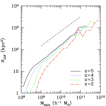
Figure 3: Mean LLS cross-section versus the mass of the closest halo at different redshifts. The black dashed line is for reference and has a logarithmic slope of $\frac{2}{3}$. The curves have a similar slope to this line, indicating that $\sigma_{\rm LLS}\propto r_{\rm vir}^{2}$. There is a clear evolution in redshift with halos of a given mass having a smaller LLS cross-section at lower redshifts. In addition, there is a cutoff at low mass which increases with decreasing redshift.

This characteristic mass and its evolution can be interpreted in terms of the photoionization of halos due to the UVB, a process described in Hoeft et al. (2006); Okamoto, Gao & Theuns (2008). In Okamoto, Gao & Theuns (2008), the authors studied the baryon fraction of halos as a function of halo mass and redshift. They found that there is a characteristic mass which evolves with redshift at which the halos retain half of the universal baryon fraction. Below this mass, the halos are unable to retain their gas due to photoheating from the UVB. Note that the reference simulation used in that work had a similar mass resolution ($2.2\times 10^{5}h^{-1}{\rm M}_{\odot}$) to the simulations used in this work so the same effect should be seen. Instead of the baryonic fraction, I use the LLS covering fraction within a virial radius:

$$f_{\rm LLS}=\frac{\sigma_{\rm LLS}}{\pi r_{\rm vir}^{2}}.$$ (10)

For large halos, this covering fraction asymptotes to a constant value which depends on redshift (see Fig. 3). I then find the characteristic mass at which the covering fraction drops to half of this asymptotic value, $M_{\frac{1}{2}}$. Below this mass, the covering fraction falls rapidly. I compare the characteristic mass derived from the LLSs covering fraction with the characteristic mass from Okamoto, Gao & Theuns (2008) in Figure 4. I find that they roughly agree and have a similar evolution with redshift which suggests that the drop in the LLS covering fraction is due to photoionization of low-mass halos. Note that this comparison is only a qualitative one since the characteristic mass as derived from the baryonic fraction is not expected to be the same as the characteristic mass as derived from the LLS covering fraction.

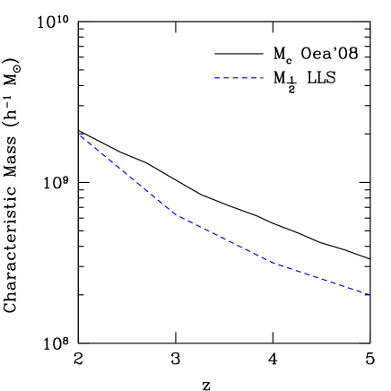
Figure 4: Characteristic mass scale for halos to retain half their gas. The solid black curve shows the characteristic mass from Okamoto, Gao & Theuns (2008), $M_{c}$, at which halos retain half of their baryonic mass. The dashed blue curve shows the characteristic mass, $M_{\frac{1}{2}}$, at which the covering fraction within the virial radius drops to half of the asymptotic value, as described in the text.

4.2 Contribution of Different Mass Halos to the LLS Population

Next, I compute how much each halo mass range contributes to the total LLS population. The cumulative contribution to the LLS incidence for halos with mass less than $M$ is given by

$$l_{\rm LLS}(<M)=\frac{c}{H_{0}}\sum_{M_{i}=M_{\rm min}}^{M}\overline{\sigma}_{\rm LLS}(M_{i},z)\overline{n}(M_{i},z),$$ (11)

where $M_{\rm min}$ is a minimum mass, given by $10^{8}h^{-1}{\rm M}_{\odot}$ in this work and $\overline{n}(M_{i},z)$ is defined as in Equation (8). This cumulative incidence is plotted in Figure 5 where it has been normalized by the total incidence. I find that a large range of halos contribute to the total LLS frequency. Furthermore, I find that for redshifts between $z=2$ and $z=5$, low-mass halos with $M<10^{10}h^{-1}{\rm M}_{\odot}$ contribute the majority of LLSs. While the contribution to the LLS population from halos with $M<10^{10}{\rm h}^{-1}{\rm M}_{\odot}$ has been studied before (i.e. Rahmati & Schaye, 2014), the mass resolution used in this work allows us to extend this to the population of LLSs residing in halos with $M<10^{9}{\rm h}^{-1}{\rm M}_{\odot}$ which contribute $\sim 30\%$ of the total LLSs at $z=3$.

This mass range is especially interesting since H₂-based models of star formation predict that these halos with $M<10^{10}h^{-1}{\rm M}_{\odot}$ will have little star formation and hence should be dark (Gnedin & Kravtsov, 2010; Kuhlen, Madau & Krumholz, 2013). The results of Figure 5 indicate that while these halos may be dark, they will contribute the majority of systems seen in surveys of LLSs.

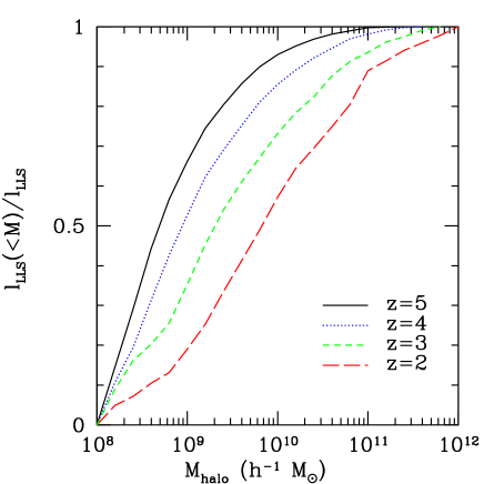
Figure 5: Cumulative LLS incidence versus halo mass at different redshifts. Note that the contribution from each mass range has been corrected by the halo mass function. While LLSs arise in a variety of systems, most LLSs arise in low-mass halos with $M<10^{10}h^{-1}M_{\odot}$. This figure also shows a clear evolution in redshift: at later times, LLSs arise in more massive halos.

4.3 Distance to the Nearest Halo

Now that I have explored the mass range of systems hosting LLSs, I will study the distance from the LLSs to the nearest halo. In Kohler & Gnedin (2007), the authors showed that the distance to the nearest halo scaled like the virial radius, although this relation had significant scatter due to the resolution of the simulation and the lack of statistics. In Figure 6, I plot the median distance to the nearest halo in units of the virial radius of the halo, as a function of halo mass. As expected from Figure 3, there is a self-similar structure where LLSs can be found at a constant fraction of the virial radius down to the cutoff mass. This plot is from the $z=3$ snapshot which has a cutoff mass of $M_{\frac{1}{2}}=6.3\times 10^{8}h^{-1}{\rm M}_{\odot}$ (see Fig. 4). Below this mass, the median distance to the nearest halo is dominated by systems outside of the virial radius and hence the distance to the nearest halo increases at low halo masses.

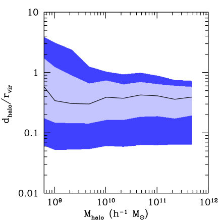
Figure 6: 3d distance to nearest halo, in units of the virial radius, as a function of halo mass. Note that this plot is made from the $z=3$ snapshot which has a characteristic mass of $6.3\times 10^{8}h^{-1}{\rm M}_{\odot}$. The black curve is the median, the light blue (dark blue) band is the 1$\sigma$ (2$\sigma$) scatter around the median. The constancy of this ratio over a wide range of masses indicates that the LLSs have a self-similar structure around their host halos where LLSs are found at the same fraction of the virial radius.

A related and important quantity is how the distance to the nearest halo depends on the column density of the absorber. In Figure 7 I plot the median distance to the nearest halo as a function of $N_{{\rm HI}}$. This shows an anti-correlation between the distance to the halo and $N_{{\rm HI}}$, i.e. stronger absorbers are closer to their host halo. This trend is very similar to what was found in Rahmati & Schaye (2014)with a fairly weak anti-correlation for LLSs which becomes stronger in the DLA regime(see Figure 2 in Rahmati & Schaye, 2014).

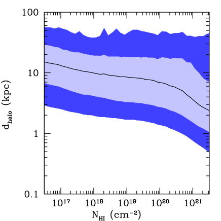
Figure 7: 3d distance to nearest halo in kpc as a function of the column density of the absorber. The black curve is the median, the light blue (dark blue) band is the 1$\sigma$ (2$\sigma$) scatter around the median. The trend shows an anti-correlation between distance and $N_{{\rm HI}}$ with stronger absorbers residing closer to their host halos.

5 Physical Properties of Individual LLSs

Now that I have explored the observed properties of LLSs, as well as the halos in which these systems reside, I will study the physical nature of individual LLSs. LLSs span a wide range of column densities: from $N_{{\rm HI}}=10^{17.2}{\rm cm}^{-2}$ to $N_{{\rm HI}}=10^{20.3}{\rm cm}^{-2}$. At the lower end of this range, the systems are mostly ionized and are believed to be in photoionization equilibrium (Schaye, 2001). As the column density increases, these systems become significantly self-shielded and become mostly neutral by the DLA threshold. In this section I will explore this transition and test the model developed in Schaye (2001).

5.1 Analytical Model

Schaye (2001) developed a simple model to describe the properties of LLSs. At low column densities, the gas is taken to be in photoionization equilibrium with the UVB, i.e.

$$\Gamma{n_{\rm HI}}=\beta_{\rm HII}n_{\rm e}n_{\rm HII}$$ (12)

where $\Gamma$ is the photoionization rate, $\beta_{\rm HII}$ is the recombination coefficient, and ${n_{\rm HI}},n_{\rm HII},n_{\rm e}$ are the number densities of HI, HII, and electrons respectively. This relation can be used to solve for the HI fraction in terms of the photoionization rate, recombination rate, and the hydrogen density. The recombination rate is a function of the temperature which can be found in Draine (2011).

In addition, Schaye (2001) argues that the characteristic size of the absorber is given by the Jeans length of the system:

$$L_{J}=t_{\rm ff}c_{\rm s}=0.52\>{\rm kpc}\>\Big{(}\frac{n_{\rm H}}{1{\rm cm}^{-3}}\Big{)}^{-1/2}T_{4}^{1/2},$$ (13)

where $T_{4}=T/10^{4}{\rm K}$ is the temperature of the gas and I have assumed that the gas is at the universal baryon fraction. The assumptions of this model are spelled out in detail in Schaye (2001) and assume that the gas in hydrostatic and photoionization equilibrium and that density distribution is uniform. Note that the temperature depends weakly on $N_{{\rm HI}}$ but is on the order of $10^{4}{\rm K}$ for LLSs. The photoionization equilibrium assumption breaks down as the system becomes significantly self-shielded and at large $N_{{\rm HI}}$, the gas becomes fully neutral. For systems at large $N_{{\rm HI}}$, assuming that the gas is fully neutral with a scale length given by the Jeans length gives the correct asymptotic behavior but not the normalization.

5.2 Characteristic Size

The model developed in Schaye (2001) assumes that the typical length of these systems is given by the Jeans length. As a measure of the characteristic size of the absorber, I take the length needed to get 90% of the total HI absorption along a line of sight. This mitigates the contribution of HI which is not associated with the LLS which can lead to artificially large sizes. This scheme was used by Prochaska & Wolfe (1997) where they faced a similar problem in measuring the velocity width from a metal-line absorption profile. I implement this method by taking 500kpc lines of sight centered on the absorber and determining the HI column density along this line of sight. I then find the distance needed to get 45% of the total $N_{{\rm HI}}$. I have tested that this characteristic length has converged by considering longer lines of sight (up to 1Mpc).

In Figure 8 I plot the median characteristic length as a function of $N_{{\rm HI}}$ along with the model from Schaye (2001). For the low $N_{{\rm HI}}$ systems, I have over-plotted the Jeans length assuming photoionization equilibrium. For the high $N_{{\rm HI}}$ systems, I over-plotted the Jeans length assuming the gas is fully neutral. At low $N_{{\rm HI}}$, I find that the model is very close to the median. Note that the model should not be expected to give an exact quantitative match but rather describe the scaling and trends of the simulation results. Most importantly, the model reproduces the scaling behavior at low $N_{{\rm HI}}$, $L_{J}\propto N_{{\rm HI}}^{-1/3}$, which follows from combining Equation (12) and Equation (13), i.e. assuming that the gas is in photoionization equilibrium with the UVB and in local hydrostatic equilibrium. This is a good assumption for optically thin gas at high redshift and explains the relation between column density and density seen in Ly$\alpha$ forest simulations (e.g. Davé et al., 2010; McQuinn, Oh & Faucher-Giguère, 2011; Altay et al., 2011; Rahmati et al., 2013a).

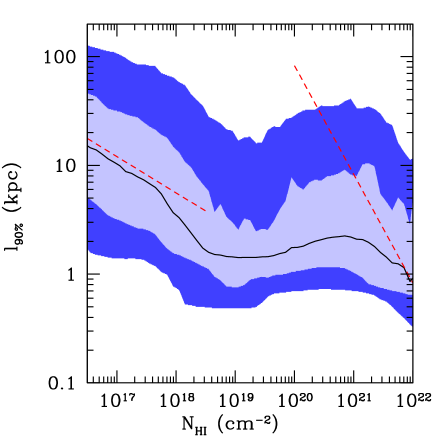
Figure 8: Absorption length for 90% of the absorption. The solid black curve is the median and the light blue (dark blue) band is the 1$\sigma$ (2$\sigma$) scatter around the median. At low $N_{{\rm HI}}$, the dashed red line is the Jeans length assuming photoionization equilibrium and $T=1.5\times 10^{4}$K - close to the average temperature in the simulation at these $N_{{\rm HI}}$. At high $N_{{\rm HI}}$, the dashed red line is the Jeans length assuming that the gas is fully neutral with an arbitrary normalization to show that the model recovers the scaling behavior.

5.3 Transition from Ionized to Neutral LLSs

As the HI column density increases from the threshold of a LLS up to a DLA, the systems go from mostly ionized to neutral due to self-shielding. In Figure 9, I plot the median HI column density versus the total hydrogen column density along 200kpc lines of sight centered on the absorber. As in the previous plots, these quantities are computed along lines of sight through the box. Note that I have plotted the total $N_{\rm H}$ on the $x$-axis to emphasize that $N_{{\rm HI}}$ depends on the total $N_{\rm H}$. Since the average HI fraction along a line of sight is given by $N_{{\rm HI}}/N_{\rm H}$, this plot also shows how the HI fraction depends on $N_{\rm H}$.

At low column density, $N_{{\rm HI}}<10^{18}{\rm cm}^{-2}$, I have included the photoionization equilibrium model with the UVB. The gas is taken to be highly ionized and in photoionization with the UVB. The column densities are thus given by $N_{{\rm HI}}=n_{\rm HI}L_{J}\propto n_{\rm H}^{\frac{3}{2}}$ and $N_{\rm H}=n_{\rm H}L_{J}\propto n_{\rm H}^{\frac{1}{2}}$ at constant temperature. Although this model does not quantitatively match the simulation result, it does reproduce the scaling behavior of $N_{{\rm HI}}\propto N_{\rm H}^{3}$. The main reason for the discrepancy is that atomic hydrogen is more localized that the total hydrogen since it must be self-shielded. As a result, for the 200 kpc line of sight used in Figure 9, $N_{\rm H}$ gets a more substantial contribution from material outside the Jeans length which offsets the relation to the right of the model at low column densities. The quantity considered below, $\langle n_{\rm H}\rangle$, avoids this problem and has a better match at low $N_{{\rm HI}}$.

Above the threshold of $N_{{\rm HI}}=10^{18}{\rm cm}^{-2}$, there is a rapid increase in $N_{{\rm HI}}$ for a small increase in $N_{\rm H}$ due to self-shielding of the gas. For the highest column density systems, $N_{{\rm HI}}>10^{20.3}{\rm cm}^{-2}$, the systems asymptote to fully atomic systems. To showcase this asymptotic behavior, I have included 3 lines in Figure 9 with successively higher neutral fractions. Note that at even higher column densities, molecular physics becomes important and non-negligible H₂ fractions make $N_{{\rm HI}}<N_{\rm H}$.

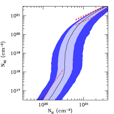
Figure 9: $N_{\rm H}$ versus $N_{{\rm HI}}$ along 200 kpc lines of sight. The solid black curve is the median and the light blue (dark blue) band is the 1$\sigma$ (2$\sigma$) scatter around the median. At low $N_{\rm H}$ I have assumed photoionization equilibrium. The dashed red line corresponds to $T=1.5\times 10^{4}$K - the average temperature at these $N_{{\rm HI}}$ in the simulation. Although the model does not quantitatively match the median, it does reproduce the scaling behavior of $N_{{\rm HI}}\propto N_{\rm H}^{3}$ which is described in the text. At large $N_{\rm H}$, the gas becomes neutral and asymptotically approaches $N_{{\rm HI}}=N_{\rm H}$ until molecular hydrogen effects and ionization from local sources become important. To guide the eye, I have included curves with $N_{{\rm HI}}=0.5N_{\rm H}$, $N_{{\rm HI}}=0.9N_{\rm H}$, and $N_{{\rm HI}}=N_{\rm H}$ which are lines of constant HI fraction. The median in the simulation is asymptoting to fully neutral gas.

A related plot found in other works (i.e. McQuinn, Oh & Faucher-Giguère, 2011; Altay et al., 2011; Rahmati et al., 2013a) is the median gas density versus $N_{{\rm HI}}$. As in these works, I compute the integral of ${n_{\rm H}}$ weighted by ${n_{\rm HI}}$:

$$\langle{n_{\rm H}}\rangle=\frac{\int{n_{\rm H}}{n_{\rm HI}}dl}{\int{n_{\rm HI}}dl}.$$ (14)

Since ${n_{\rm HI}}$ is more sharply peaked than ${n_{\rm H}}$ due to self-shielding, this effectively selects the central part of the absorber. I show the median $\langle{n_{\rm H}}\rangle$ in Figure 10. I find that the photoionization equilibrium model reproduces the properties well at low $N_{{\rm HI}}$. It matches the scaling behavior of $\langle{n_{\rm H}}\rangle\propto N_{{\rm HI}}^{2/3}$ derived from Equation (12) and Equation (13). Above $N_{{\rm HI}}=10^{18}{\rm cm}^{-2}$, self-shielding becomes important and there is a large increase in $N_{{\rm HI}}$ for a small increase in $\langle{n_{\rm H}}\rangle$. At the highest $N_{{\rm HI}}$, the gas is expected to be fully neutral and the model from Schaye (2001) predicts that $\langle{n_{\rm H}}\rangle\propto N_{{\rm HI}}^{2}$. As in Figure 8, the median does not asymptote to the model curve.

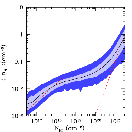
Figure 10: $n_{\rm H}$ weighted by $n_{\rm HI}$ averaged along 200 kpc sightlines versus $N_{{\rm HI}}$. The solid black curve is the median and the light blue (dark blue) band is the 1$\sigma$ (2$\sigma$) scatter around the median. At low $N_{{\rm HI}}$, the dashed red curve shows the prediction from the photoionization equilibrium model with $T=1.5\times 10^{4}$K which reproduces the scaling behavior of the median. At large $N_{{\rm HI}}$, the dashed red curves show the prediction from fully neutral gas with an arbitrary normalization to show the model recovers the scaling behavior

For ease in comparison with other work, I also include a related quantity which is the $n_{\rm HI}$ weighted $x_{\rm HI}$ fraction in Figure 11 (McQuinn, Oh & Faucher-Giguère, 2011; Altay et al., 2011). The comparison between the results of those works and this work is discussed in Section 8.

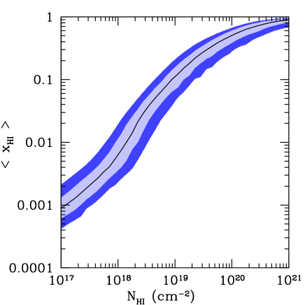
Figure 11: $x_{\rm HI}$ weighted by $n_{\rm HI}$ averaged along 200 kpc sightlines versus $N_{{\rm HI}}$. The solid black curve is the median and the light blue (dark blue) band is the 1$\sigma$ (2$\sigma$) scatter around the median.

5.4 Effect of Self-Shielding on the Column Density Distribution

In Section 3, we saw that the HI column density distribution has a flattening at $N_{{\rm HI}}\sim 10^{18}{\rm cm}^{-2}$ which has been attributed to self-shielding (McQuinn, Oh & Faucher-Giguère, 2011; Altay et al., 2011; Rahmati et al., 2013a). A priori it is unclear that this flattening is only due to self-shielding and not due to some feature in the total hydrogen column density distribution. This can be checked by comparing the HI column density distribution, $f_{\rm HI}(N_{{\rm HI}})$, and the total hydrogen column density distribution $f_{\rm H}(N_{\rm H})$, where I have included additional subscripts to emphasize that they are different distributions. These two distributions are related by

$$f_{\rm HI}(N_{{\rm HI}})=f_{\rm H}(N_{\rm H})\frac{dN_{\rm H}}{dN_{{\rm HI}}}.$$ (15)

The relation between $N_{{\rm HI}}$ and $N_{\rm H}$ is shown in Figure 9. Using the median of this relation, $\frac{dN_{\rm H}}{dN_{{\rm HI}}}$ can be computed. Furthermore, $f_{\rm H}(N_{\rm H})$ can be computed in the simulation and then Equation (15) can be used to compute $f_{\rm HI}(N_{{\rm HI}})$. The result of this procedure is shown in Figure 12. $f(N_{\rm H})$ is a power-law over the range in which the transition between ionized and self-shielding occurs. Therefore, these simulations show that the feature at $N_{{\rm HI}}\sim 10^{18}{\rm cm}^{-2}$ is a signature of self-shielding and not the distribution of the total hydrogen at the corresponding column density.

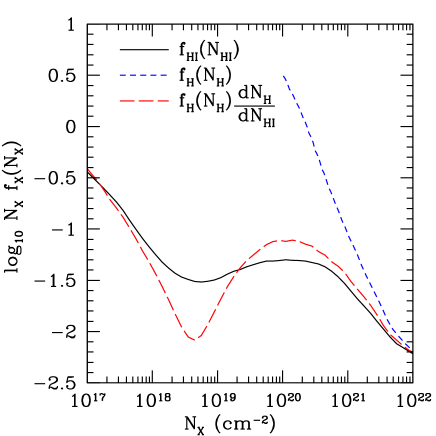
Figure 12: HI column density distribution and H column density distribution. The black solid curve shows the HI column density distribution as computed from the simulation. The blue, short-dashed, curve shows the total hydrogen column density distribution as computed in the simulation. Finally, the red long-dashed curve shows the result of taking the median profile in Figure 9 to compute $\frac{dN_{\rm H}}{dN_{{\rm HI}}}$ and then computing the HI column density distribution using Equation (15). Note that the median relation between $N_{{\rm HI}}$ and $N_{\rm H}$ was smoothed over in order to reduce the noise in the derivative.

5.5 Photoionization Rate

In the limit where we can neglect radiative recombination and local sources of radiation, the photoionization rate of LLSs directly measures the self-shielding of the LLS against the UVB. Since the distance of an absorber from its host galaxy is anti-correlated with its HI column density, as shown in Figure 7, low $N_{{\rm HI}}$ systems will not be significantly affected by the local radiation from their host halo. The decrease in the photoionization rate in a LLS allows us to measure the effective shielding of the LLS against the UVB. In Figure 13, I plot the photoionization rate averaged along lines of sight through the LLS, weighted by ${n_{\rm HI}}$:

$$\langle\Gamma\rangle=\frac{\int\Gamma(l)n_{{\rm HI}}dl}{\int n_{{\rm HI}}dl}.$$ (16)

If only the contribution from the UVB is considered, this integral can be solved for a monochromatic UVB. In this limit, the differential optical depth can be written as $d\tau={n_{\rm HI}}\sigma_{\rm HI}dl$ and get

$$\langle\Gamma\rangle=\frac{\int\Gamma_{0}e^{-\tau}\sigma_{\rm HI}^{-1}d\tau}{N_{{\rm HI}}},$$ (17)

where $\Gamma(\tau)=\Gamma_{0}e^{-\tau}$ and $\sigma_{\rm HI}$ is independent of $\tau$. This then gives

$$\langle\Gamma\rangle=\Gamma_{0}\frac{1-e^{-N_{{\rm HI}}\sigma_{\rm HI}}}{N_{{\rm HI}}\sigma_{\rm HI}}.$$ (18)

In Figure 13, I include this model for a slab with column density $N_{{\rm HI}}/2$ and find that a value of $\sigma=10^{-17.7}{\rm cm}^{2}$ provides a fairly good fit at low $N_{{\rm HI}}$ although it does not match the slope at large $N_{{\rm HI}}$. I use a column density of $N_{{\rm HI}}/2$ since the LLS is illuminated on all sides by the UVB and this model assumes that the LLS is being illuminated from one direction. The difference between this model and the median photoionization rate in the simulation for $N_{{\rm HI}}>10^{19}{\rm cm}^{-2}$ is due to the increasingly important effects of radiative recombination and local radiation as $N_{{\rm HI}}$ increases (i.e. Miralda-Escudé, 2005; Schaye, 2006; Rahmati et al., 2013b; Rahmati & Schaye, 2014). However, this effect is unimportant for determining the effective shielding of the LLS which is determined at lower column densities.

I also include a model for the average photoionization rate for a slab with column density $N_{{\rm HI}}/2$ illuminated on one side by the UVB using CLOUDY v13.01 (Ferland et al., 2013). For this model, I set up a slab with a plane-parallel geometry, irradiated by the Haardt-Madau background given in Haardt & Madau (2001), with appropriate helium and metal abundances. I varied the hydrogen density ($n_{\rm H}\in[10^{-3},10^{-1}]{\rm cm}^{-3}$) and the metallicity ($Z/Z_{\odot}\in[10^{-3},10^{-1}]$) and computed the HI photoionization rate as a function of HI column density through the slab. I found that this relationship was robust and did not depend on the HI density or metallicity. This result gives the long-dashed green curve in Figure 13 which can be compared to the photoionization rate in actual simulations. This model has an effective cross-section of $\sigma_{\rm HI}=10^{-17.6}{\rm cm}^{2}$ at low column densities. Interestingly, this model does not quantitatively match the absorption seen in the simulation. This discrepancy is due to the anisotropy of the LLS which I will discuss in the next section.

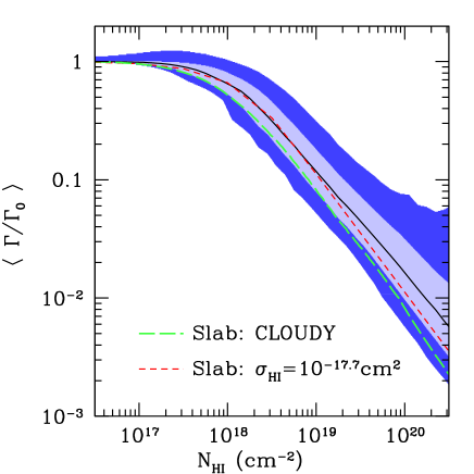
Figure 13: Median photoionization rate versus $N_{{\rm HI}}$. The photoionization rate is averaged along sightlines and weighted by the HI density. The solid black curve is the median and the light blue (dark blue) band is the 1$\sigma$ (2$\sigma$) scatter around the median. The short-dashed red curve is the model of the photoionization rate from Equation (18) which assumes a mono-chromatic UVB with $\sigma_{\rm HI}=10^{-17.7}{\rm cm}^{2}$ and has a column density of $N_{{\rm HI}}/2$. The long-dashed green line comes from computing the average photoionization rate, Equation (16), of a slab with column density $N_{{\rm HI}}/2$ illuminated by the UVB and was done with CLOUDY. These models are discussed further in the text.

6 Anisotropic Shielding of LLSs

In the previous section, I tested the model developed in Schaye (2001) and found that it successfully reproduced may of the properties of LLSs. In this model, LLSs are characterized by a single column density and the self-shielding of the absorber depends on this quantity. However, for a non-spherical absorber the column density will depend on the angular direction. To test the importance of this column density variation, I first identified the centers of LLS by finding the maximum density along a line of sight. Around this maximum, I then compute the column density along the 6 cartesian directions originating from this point to determine the HI column density in these 6 directions. In Figure 14, I show the column density along the original line of sight, $N_{{\rm HI}}$, versus the difference between $N_{{\rm HI}}$ and the minimum/maximum column density in the other 6 cartesian directions.

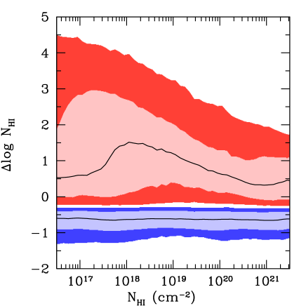
Figure 14: Comparison of the difference between the column density along a line of sight and the column density along different directions originating from the absorber. The red shaded (upper) region shows the 1 and 2$\sigma$ scatter of the difference between the maximum $N_{{\rm HI}}$ and the blue shaded (lower) region shows the 1 and 2$\sigma$ scatter of the minimum $N_{{\rm HI}}$ along the 6 cartesian directions originating at the center of the absorber. The black curves in the center of each region show the median.

Note that the column density on the $x$ axis is the column density through the entire system. This was chosen to highlight the difference between the observed $N_{{\rm HI}}$ of a system along a random line of sight, and the characteristic minimum/maximum $N_{{\rm HI}}$ between the center of the absorber and the UVB.

Figure 14 shows that if a random line of sight in the system has a column density of $N_{{\rm HI}}$, on average there will be a line of sight originating from the center of that system with a column density 0.6-0.7 dex lower, approximately $N_{{\rm HI}}/4$. As a result, systems will be more ionized than naively expected from the column density in a single direction. This result is important for understanding the column density distribution (Fig. 2), as well as the relationship between $N_{{\rm HI}}$ and $N_{\rm H}$ (Fig. 9).

In Figure 15, I compare the average photoionization rate along a cartesian direction with the average rate along the direction with the lowest $N_{{\rm HI}}$. Since the absorbers are randomly oriented with respect to the box, this cartesian direction probes an effectively random direction with respect to the absorber. The average photoionization along this direction is given by the black solid curve. Fitting this curve using Equation (18) gives an effective cross-section of $\sigma_{\rm HI}=10^{-17.7}{\rm cm}^{2}$ at low column densities. The second direction is the direction originating from the center of the LLS with the lowest $N_{{\rm HI}}$. The short-dashed blue curve shows the average photoionization rate versus column density along this direction. I also include a slab model using the UVB in the simulation. This is done using CLOUDY as I described in Section 5 and is given by the long-dashed red curve.

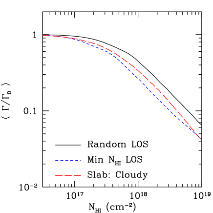
Figure 15: Photoionization rate versus $N_{{\rm HI}}$ in two different directions. The solid black curve is the median of the photoionization along a a specific cartesian direction and hence along an effectively random direction. As described in the text, the short-dashed blue curve is the median along the direction with the minimum $N_{{\rm HI}}$ originating from the center of the LLS. The long-dashed red curve is the photoionization rate from CLOUDY assuming the Haardt-Madau background at $z=3$ (Haardt & Madau, 2001).

By comparing the curves in Figure 15, I find that the photoionization rate from the slab model in CLOUDY falls between the rate along a random direction and the rate along the minimum direction in the simulation. This comparison is useful since it shows that if one takes a random line of sight through a LLS, the gas along this line of sight is less shielded than one would expect from the HI column density. This makes sense since, on average, there will be a line of sight to the UVB with a significantly lower column density (see Fig. 14) allowing for more photoionization than naively expected. Likewise, for gas along the direction with the lowest column density, there will be lines of sight with higher column densities which will result in a lower photoionization rate than expected.

7 Effective Shielding of LLSs

Putting together the results of Section 5 and Section 6, I find that the self-shielding of LLSs against the UVB is less than naively expected. Given a LLS with column density $N_{{\rm HI}}$, one would expect that this system is shielded by an optical depth of $\tau=N_{{\rm HI}}\sigma_{\rm HI}$, where $\sigma_{\rm HI}$ is an effective cross-section of HI to the UVB. Since the self-shielding of LLSs is known to flatten the column density distribution (i.e. Altay et al., 2011; McQuinn, Oh & Faucher-Giguère, 2011; Rahmati et al., 2013a, or Section 5.5 of this work), it is important to understand at what column density one should expect self-shielding to become important.

There are three effects which lower the amount of shielding. First, as I discussed in Section 5, since a LLS is bathed in the UVB from all sides, a system with a column density of $N_{{\rm HI}}$ is effectively only shielded by a column density of $N_{{\rm HI}}/2$. Second, the UVB is not monochromatic but has a spectrum which extends to high energies. Since the cross-section of HI decreases with increasing energy, these photons can penetrate deeper into the cloud and lower the effective cross-section of LLS to the UVB. As I showed in Figure 15, the effective cross-section against the UVB at $z=3$ is $\sigma_{\rm HI}\approx 10^{-17.6}{\rm cm}^{-2}$, 0.4 dex lower than the cross-section at the Lyman limit. Lastly, I investigated the effect of the anisotropy of the LLS in Section 6 and found that, on average, a LLS with a column density of $N_{{\rm HI}}$ will have a line of sight with column density $N_{{\rm HI}}/4$ from the center of the LLS to the UVB, i.e. half of what one would expect if the LLS was isotropic. This anisotropy means that an average LLS will be less shielded than expected from the column density. In Figure 15, I found that this results in a $0.1-0.2$ dex decrease in the optical depth as compared to a uniform slab.

Altogether, these three effects mean than a LLS need to have a column density of $N_{{\rm HI}}\sim 10^{18}{\rm cm}^{-2}$ in order to have an optical depth of unity. Since the flattening of the column density distribution is due to this self-shielding, this means that we should expect the column density distribution to start flattening around $N_{{\rm HI}}\sim 10^{18}{\rm cm}^{-2}$, as I find in Figure 2. In addition, the onset of self-shielding can clearly be seen in the relation between $N_{{\rm HI}}$ and $N_{\rm H}$ in Figure 9. Note that the effective cross-section of HI also depends weakly on the redshift of the LLS since the spectral shape of the UVB changes slowly with redshift.

8 Comparison with Previous Work

Both LLSs and DLAs have received significant attention in the literature and attempts are now being made to quantitatively match observations. In this section, I will compare the results in this work to papers which have made a similar attempt to understand the properties of LLSs.

Kohler & Gnedin (2007) studied LLSs using simulations which had lower spatial and mass resolution than the simulations in this work. They found many of the same trends found here although they were limited on the low-mass end. They also studied the properties of absorbers as a function of their parent halo and found that LLSs reside in halos with a large range of masses and concluded that the majority of LLSs do not reside in very low-mass halos. As in this work, they found that LLSs remain ionized up to fairly high column densities, $N_{{\rm HI}}=10^{20}{\rm cm}^{-2}$. Despite including many of the physical mechanisms needed to model the ionization state of the gas, their column density distribution did not show any signs of self-shielding around $N_{{\rm HI}}=10^{18}{\rm cm}^{-2}$.

McQuinn, Oh & Faucher-Giguère (2011) studied LLSs using simulations with a similar simulation volume as this work. They found a similar HI column density distribution as was found in this work, with significant flattening due to self-shielding starting a little above $N_{{\rm HI}}\sim 10^{18}{\rm cm}^{-2}$. They also made comparisons to the model in Schaye (2001) and found that this model had a qualitative agreement with their results. Just as in this work, they found that LLSs remain ionized up to high column densities, as can be seen in the middle panel of Figure 5 in McQuinn, Oh & Faucher-Giguère (2011) , where they have a $n_{\rm HI}$ weighted neutral fraction of $\sim 0.1$ at $N_{{\rm HI}}=10^{19}{\rm cm}^{-2}$, consistent with the neutral fraction reported in Figure 11 of this work.

Altay et al. (2011) studied both LLSs and DLAs and found a nice agreement with observed column density distribution over a wide range of $N_{{\rm HI}}$ and find self-shielding starts to flatten the HI column density distribution above $N_{{\rm HI}}=10^{18}{\rm cm}^{-2}$. Interestingly, the LLSs in their simulations are significantly less ionized than in this work or in McQuinn, Oh & Faucher-Giguère (2011). The left panel of Figure 3 in that works shows that the $n_{\rm HI}$ weighted neutral fraction at $N_{{\rm HI}}=10^{19}{\rm cm}^{-2}$ is approximately -0.2 dex, as compared to the -1 dex reported in McQuinn, Oh & Faucher-Giguère (2011) and Figure 11 of this work. Despite this difference in the ionization fraction, their relation between $\langle n_{\rm H}\rangle$ versus $N_{{\rm HI}}$ is very similar to what was found in this work in Figure 10.

Rahmati et al. (2013a) studied the redshift evolution of the column density distribution and found a similar evolution as to Figure 2. While the amplitude decreases with decreasing redshift, they find that the column density distribution becomes slightly shallower at lower redshifts and low column densities. As was discussed in Section 3.4 , the overall normalization of their HI column density distribution evolves more than this work between $z=5$ and $z=3$. This is likely due to the same reason this work had difficulty reproducing the frequency of LLSs at high-redshift in Figure 1: since this work uses zoom-in simulations, it does not capture the large-scale filamentary structure at high redshift.

Rahmati & Schaye (2014) discussed many of the same properties of LLSs as in this work using fixed dark matter particle mass of $6.3\times 10^{6}$ h${}^{-1}M_{\odot}$ ,as opposed to the zoom-in simulations used in this work. The comparison between this work and Rahmati & Schaye (2014) provides a good test of the assumption that the zoom-in region is not overly biased. The cumulative LLS incidence with respect to halo mass is also computed in the top right panel of Figure 6 inRahmati & Schaye (2014) and shows that there is not a large contribution from halos above $10^{12}M_{\odot}$, a range which is inaccessible with the zoom-in simulations used in this work. On the low-mass end, the simulations show that there is a significant contribution from halos below a halo mass of $10^{10}M_{\odot}$, in agreement with Figure 5 of this work. Rahmati & Schaye (2014) also studied the impact parameter of LLSs and found similar results to Figure 7 an anti-correlation between $N_{\rm HI}$ and the distance to the nearest halo.

9 Summary and Conclusion

In this work, I have explored the properties of LLSs using cosmological zoom-in simulations which include on the fly radiative transfer and have high mass resolution. The simulations in this work reproduce the observed incidence frequency of LLSs as well as the HI column density distribution, indicating that the simulations are effectively modeling LLSs.

Using these simulations, I investigated the host halos of LLSs. The high mass resolution of these simulations allowed me to investigate the LLS content of halos down to $10^{8}{\rm h}^{-1}M_{\odot}$. These results showed that halos have a nearly constant covering fraction of LLSs within their virial radius over a wide range of halo masses, similar to the results in Fumagalli et al. (2014). However, it is important to note that the simulations use in this work, as well as those in Fumagalli et al. (2014) use inefficient feedback which leads an overproduction of stellar mass in the halos of interest. As has been recently shown in Faucher-Giguère et al. (2015) and Rahmati et al. (2015), including more efficient feedback which is needed to produce realistic stellar masses also increases the covering fraction of LLSs and boosts it to values significantly higher than what is found in this work and in Fumagalli et al. (2014). Efficient feedback will likely affect many of the properties of LLSs and this will be investigated in future work.

In addition to this near-constant covering fraction, there is a cutoff at low halo masses which increases as the redshift decreases. I argued that this evolution of the cutoff is real since the simulations have the necessary mass resolution to adequately model these halos and that the evolution can be explained by the photoionization of gas in the galaxy due to the UVB. In addition, I found that between $z=2-5$, more than $50\%$ of LLSs reside in halos with $M<10^{10}{\rm h}^{-1}M_{\odot}$. This is especially interesting since H₂-based star formation models predict that these galaxies will be dark (i.e. Gnedin & Kravtsov, 2010; Kuhlen, Madau & Krumholz, 2013). As a result, absorption line studies of LLSs will be an important testing ground for simulations since they probe a large reservoir of gas which will be difficult to detect with other means.

Next, I investigated the properties of individual LLSs. I tested a simple model from Schaye (2001) and found that it reproduced the characteristic size and HI fraction of LLSs well for $N_{{\rm HI}}<10^{18}{\rm cm}^{-2}$. Above this threshold, the gas is no longer optically thin and the model is no longer valid. However, in the DLA regime, the gas is almost entirely neutral so the simple model is justified once again with a scale length given by the Jeans length. Using the relation between $N_{{\rm HI}}$ and $N_{\rm H}$, I showed how onset of self-shielding at $N_{{\rm HI}}=10^{18}{\rm cm}^{-2}$ is responsible for the flattening of the HI column density distribution which has also been shown in McQuinn, Oh & Faucher-Giguère (2011); Altay et al. (2011); Rahmati et al. (2013a).

Lastly, I studied why this self-shielding occurs at a higher value than one might naively expect for LLSs. While the hard spectrum from the UVB accounts for most of the difference, there is also a significant effect from the anisotropic structure of LLSs. For an absorber with a column density of $N_{{\rm HI}}$ in a given direction, I found that on average, there are lines of sight which have significantly less shielding to the UVB. This results in the absorber being more ionized than expected from the column density. Together, these effects result in the onset of self-shielding being pushed to $N_{{\rm HI}}=10^{18}{\rm cm}^{-2}$. One consequence of this result is that if one can independently constrain the UVB or the anisotropic structure of LLSs, the other quantity can be constrained by measuring the column density at which self-shielding kicks in.

I would like to thank the anonymous referee for a thoughtful and thorough report which improved the quality of the paper. I would like to acknowledge helpful comments from Nick Gnedin, Andrey Kravtsov, Stephan Meyer, Dan Holz, Tom Witten, Oscar Agertz and Benedikt Diemer. This work was supported in part by the NSF grant AST-0908063, and by the NASA grant NNX-09AJ54G. The simulations used in this work have been performed on the Joint Fermilab - KICP Supercomputing Cluster, supported by grants from Fermilab, Kavli Institute for Cosmological Physics, and the University of Chicago. This work made extensive use of the NASA Astrophysics Data System and the arXiv.org preprint server. I made use of the CAMB code to generate power spectra in the course of this work.

References

- Abel & Mo (1998) Abel T., Mo H. J., 1998, ApJ, 494, L151
- Altay et al. (2011) Altay G., Theuns T., Schaye J., Crighton N. H. M., Dalla Vecchia C., 2011, ApJ, 737, L37+
- Davé et al. (2010) Davé R., Oppenheimer B. D., Katz N., Kollmeier J. A., Weinberg D. H., 2010, MNRAS, 408, 2051
- Draine (2011) Draine B. T., 2011, Physics of the Interstellar and Intergalactic Medium
- Faucher-Giguère et al. (2015) Faucher-Giguère C.-A., Hopkins P. F., Kereš D., Muratov A. L., Quataert E., Murray N., 2015, MNRAS, 449, 987
- Ferland et al. (2013) Ferland G. J. et al., 2013, Rev. Mexicana Astron. Astrofis., 49, 137
- Fumagalli et al. (2014) Fumagalli M., Hennawi J. F., Prochaska J. X., Kasen D., Dekel A., Ceverino D., Primack J., 2014, ApJ, 780, 74
- Fumagalli et al. (2011) Fumagalli M., Prochaska J. X., Kasen D., Dekel A., Ceverino D., Primack J. R., 2011, MNRAS, 418, 1796
- Gardner et al. (1997) Gardner J. P., Katz N., Hernquist L., Weinberg D. H., 1997, ApJ, 484, 31
- Gardner et al. (2001) Gardner J. P., Katz N., Hernquist L., Weinberg D. H., 2001, ApJ, 559, 131
- Gnedin (2014) Gnedin N. Y., 2014, ApJ, 793, 29
- Gnedin & Abel (2001) Gnedin N. Y., Abel T., 2001, New Astronomy, 6, 437
- Gnedin & Kravtsov (2010) Gnedin N. Y., Kravtsov A. V., 2010, ApJ, 714, 287
- Gnedin & Kravtsov (2011) Gnedin N. Y., Kravtsov A. V., 2011, ApJ, 728, 88
- Haardt & Madau (2001) Haardt F., Madau P., 2001, in Clusters of Galaxies and the High Redshift Universe Observed in X-rays, Neumann D. M., Tran J. T. V., eds.
- Hoeft et al. (2006) Hoeft M., Yepes G., Gottlöber S., Springel V., 2006, MNRAS, 371, 401
- Iliev et al. (2006) Iliev I. T. et al., 2006, MNRAS, 371, 1057
- Iliev et al. (2009) Iliev I. T. et al., 2009, MNRAS, 400, 1283
- Katz et al. (1996) Katz N., Weinberg D. H., Hernquist L., Miralda-Escude J., 1996, ApJ, 457, L57
- Kohler & Gnedin (2007) Kohler K., Gnedin N. Y., 2007, ApJ, 655, 685
- Kravtsov (1999) Kravtsov A. V., 1999, PhD thesis, NEW MEXICO STATE UNIVERSITY
- Kravtsov, Klypin & Hoffman (2002) Kravtsov A. V., Klypin A., Hoffman Y., 2002, ApJ, 571, 563
- Kuhlen, Madau & Krumholz (2013) Kuhlen M., Madau P., Krumholz M. R., 2013, ApJ, 776, 34
- Leitherer et al. (1999) Leitherer C. et al., 1999, ApJS, 123, 3