Perturbed Message Passing for Constraint Satisfaction Problems

Abstract

We introduce an efficient message passing scheme for solving Constraint Satisfaction Problems (CSPs), which uses stochastic perturbation of Belief Propagation (BP) and Survey Propagation (SP) messages to bypass decimation and directly produce a single satisfying assignment. Our first CSP solver, called Perturbed Belief Propagation, smoothly interpolates two well-known inference procedures; it starts as BP and ends as a Gibbs sampler, which produces a single sample from the set of solutions. Moreover we apply a similar perturbation scheme to SP to produce another CSP solver, Perturbed Survey Propagation. Experimental results on random and real-world CSPs show that Perturbed BP is often more successful and at the same time tens to hundreds of times more efficient than standard BP guided decimation. Perturbed BP also compares favorably with state-of-the-art SP-guided decimation, which has a computational complexity that generally scales exponentially worse than our method (w.r.t. the cardinality of variable domains and constraints). Furthermore, our experiments with random satisfiability and coloring problems demonstrate that Perturbed SP can outperform SP-guided decimation, making it the best incomplete random CSP-solver in difficult regimes.

Keywords: Constraint Satisfaction Problem, Message Passing, Belief Propagation, Survey Propagation, Gibbs Sampling, Decimation

1 Introduction

Probabilistic Graphical Models (PGMs) provide a common ground for recent convergence of themes in computer science (artificial neural networks), statistical physics of disordered systems (spin-glasses) and information theory (error correcting codes). In particular, message passing methods have been successfully applied to obtain state-of-the-art solvers for Constraint Satisfaction Problems (Mézard et al., 2002)

The PGM formulation of a CSP defines a uniform distribution over the set of solutions, where each unsatisfying assignment has a zero probability. In this framework, solving a CSP amounts to producing a sample from this distribution. To this end, usually an inference procedure estimates the marginal probabilities, which suggests an assignment to a subset of the most biased variables. This process of sequentially fixing a subset of variables, called decimation, is repeated until all variables are fixed to produce a solution. Due to inaccuracy of the marginal estimates, this procedure gives an incomplete solver (Kautz et al., 2009), in the sense that the procedure’s failure is not a certificate of unsatisfiability. An alternative approach is to use message passing to guide a search procedure that can back-track if a dead-end is reached (e.g.,  Kask et al., 2004; Parisi, 2003). Here using a branch and bound technique and relying on exact solvers, one may also determine when a CSP is unsatisfiable.

The most common inference procedure for this purpose is Belief Propagation (Pearl, 1988). However, due to geometric properties of the set of solutions (Krzakala et al., 2007) as well as the complications from the decimation procedure (Coja-Oghlan, 2011; Kroc et al., 2009), BP-guided decimation fails on difficult instances. The study of the change in the geometry of solutions has lead to Survey Propagation (Braunstein et al., 2002) which is a powerful message passing procedure that is slower than BP (per iteration) but typically remains convergent, even in many situations when BP fails to converge.

Using decimation, or other search schemes that are guided by message passing, usually requires estimating marginals or partition functions, which is harder than producing a single solution (Valiant, 1979). This paper introduces a message passing scheme to eliminate this requirement, therefore also avoiding the complications of applying decimation. Our alternative has advantage over both BP- and SP-guided decimation when applied to solve CSPs. Here we consider BP and Gibbs Sampling (GS) updates as operators – ${\Phi}$ and ${\Psi}$ respectively – on a set of messages. We then consider inference procedures that are convex combination (i.e., $\gamma{\Psi}+(1-\gamma){\Phi}$) of these two operators. Our CSP solver, Perturbed BP, starts at $\gamma=0$ and ends at $\gamma=1$, smoothly changing from BP to GS, and finally producing a sample from the set of solutions. This change amounts to stochastic biasing the BP messages towards the current estimate of marginals, where this random bias increases in each iteration. This procedure is often much more efficient than BP-guided decimation (BP-dec) and sometimes succeeds where BP-dec fails. Our results on random CSPs (rCSPs) show that Perturbed BP is competitive with SP-guided decimation (SP-dec) in solving difficult random instances.

Since SP can be interpreted as BP applied to an “auxiliary” PGM (Braunstein and Zecchina, 2003), we can apply the same perturbation scheme to SP, which we call Perturbed SP. Note that this system, also, does not perform decimation and directly produce a solution (without using local search). Our experiments show that Perturbed SP is often more successful than both SP-dec and Perturbed BP in finding satisfying assignments.

Stochastic variations of BP have been previously proposed to perform inference in graphical models (e.g.,  Ihler and Mcallester, 2009; Noorshams and Wainwright, 2013). However, to our knowledge, Perturbed BP is the first method to directly combine GS and BP updates.

In the following, Section 1.1 introduces PGM formulation of CSP using factor-graph notation. Section 1.2 reviews the BP equations and decimation procedure, then Section 1.3 casts GS as a message update procedure. Section 2 introduces Perturbed BP as a combination of GS and BP. Section 2.1 compares BP-dec and Perturbed BP on benchmark CSP instances, showing that our method is often several folds faster and more successful in solving CSPs. Section 3 overviews the geometric properties of the set of solutions of rCSPs, then reviews first order Replica Symmetry Breaking Postulate and the resulting SP equations for CSP. Section 3.2 introduces Perturbed SP and Section 3.3 presents our experimental results for random satisfiability and random coloring instances close to the unsatisfiability threshold. Finally, Section 3.4 further discusses the behavior of decimation and perturbed BP in the light of a geometric picture of the set of solutions and the experimental results.

1.1 Factor Graph Representation of CSP

Let $x=(x_{1},x_{2},\ldots,x_{N})$ be a tuple of $N$ discrete variables $x_{i}\in\mathcal{X}_{i}$, where each $\mathcal{X}_{i}$ is the domain of $x_{i}$. Let $I\subseteq\mathcal{N}=\{1,2,\ldots,N\}$ denote a subset of variable indices and $x_{I}\!=\!\{x_{i}\!\mid\!i\in I\}$ be the (sub)tuple of variables in $x$ indexed by the subset $I$. Each constraint $C_{I}(x_{I}):\;\big{(}\prod_{i\in I}\mathcal{X}_{i}\big{)}\rightarrow\{0,1\}$ maps an assignment to 1 iff that assignment satisfies that constraint. Then the normalized product of all constraints defines a uniform distribution over solutions:

$$\mu(x)\quad\triangleq\quad\frac{1}{Z}\prod_{I}C_{I}(x_{I})$$ (1)

where the partition function $Z\;=\;\sum_{\mathcal{X}}\prod_{I}C_{I}(x_{I})$ is equal to the number of solutions. Notice that $\mu(x)$ is non-zero iff all of the constraints are satisfied – that is $x$ is a solution. With slight abuse of notation we will use probability density and probability distribution interchangeably.

Example 1 ($q$-COL:)

Here, $x_{i}\in\mathcal{X}_{i}=\{1,\ldots,q\}$ is a q-ary variable for each $i\in\mathcal{N}$, and we have $M$ constraints; each constraint $C_{i,j}(x_{i},x_{j})=1-\delta(x_{i},x_{j})$ depends only on two variables and is satisfied iff the two variables have different values (colors). Here $\delta(x,x^{\prime})$ is equal to 1 if $x=x^{\prime}$ and 0 otherwise.

This model can be conveniently represented as a bipartite graph, known as a factor graph (Kschischang et al., 2001), which includes two sets of nodes: variable nodes $x_{i}$, and constraint (or factor) nodes $C_{I}$. A variable node $i$ (note that we will often identify a variable “$x_{i}$” with its index “$i$”) is connected to a constraint node $I$ if and only if $i\in I$. We will use $\partial$ to denote the neighbors of a variable or constraint node in the factor graph – that is $\partial I=\{i\;\mid\;i\in I\}$ (which is the set $I$) and $\partial i=\{I\;\mid\;i\in I\}$. Finally we use $\Delta i$ to denote the Markov blanket of node $x_{i}$ ($\Delta i=\{j\in\partial I\;\mid\;I\in\partial i,j\neq i\}$).

The marginal of $\mu(\cdot)$ for variable $x_{i}$ is defined as

$$\mu(x_{i})\;\triangleq\;\sum_{\mathcal{X}_{\mathcal{N}\setminus i}}\mu(x)$$

where the summation above is over all variables but $x_{i}$. Below, we use $\widehat{\mu}(x_{i})$ to denote an estimate of this marginal. Finally, we use $\mathcal{S}$ to denote the (possibly empty) set of solutions $\mathcal{S}=\{x\in\mathcal{X}\;\mid\;\mu(x)\neq 0\}$.

Example 2 ($\kappa$-SAT:)

All variables are binary ($\mathcal{X}_{i}=\{True,False\}$) and each clause (constraint $C_{I}$) depends on $\kappa=|\partial I|$ variables. A clause evaluates to 0 only for a single assignment out of $2^{\kappa}$ possible assignment of variables (Garey and Johnson, 1979).

Consider the following 3-SAT problem over 3 variables with 5 clauses:

$$SAT(x)\;=\;\underbrace{(\neg x_{1}\vee\neg x_{2}\vee x_{3})}_{C_{1}}\wedge\underbrace{(\neg x_{1}\vee x_{2}\vee x_{3})}_{C_{2}}\wedge\underbrace{(x_{1}\vee\neg x_{2}\vee x_{3})}_{C_{3}}\wedge\underbrace{(\neg x_{1}\vee x_{2}\vee\neg x_{3})}_{C_{4}}\wedge\underbrace{(x_{1}\vee\neg x_{2}\vee\neg x_{3})}_{C_{5}}$$ (2)

The constraint corresponding to the first clause takes the value $1$, except for $x=\{True,True,False\}$, in which case it is equal to $0$. The set of solutions for this problem is given by:
$\mathcal{S}=\big{\{}(True,True,True),\;(False,False,False),\;(False,False,True)\big{\}}$. Figure 1 shows the solutions as well as the corresponding factor graph.

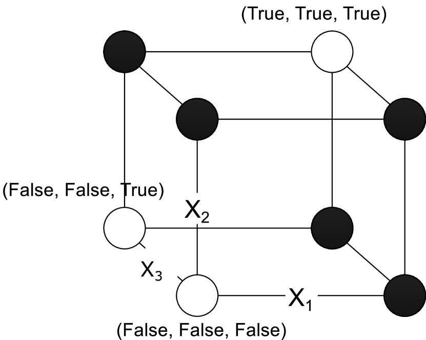
(a)

(b)

Figure 1: (a) The set of all possible assignments to 3 variables. The solutions to the 3-SAT problem of Eq 2 are in white circles. (b) The factor-graph corresponding to the 3-SAT problem of Eq 2. Here each factor prohibits a single assignment.

1.2 Belief Propagation-guided Decimation

Belief Propagation (Pearl, 1988) is a recursive update procedure that sends a sequence of messages from variables to constraints ($\nu_{i\to{I}}$) and vice-versa ($\nu_{{I}\to i}$):

$$\nu_{i\to{I}}(x_{i})\;\propto\;\prod_{J\in\partial i\setminus I}\nu_{J\to i}(x_{i})$$ (3)

$$\nu_{I\to i}(x_{i})\;\propto\;\sum_{x_{I\setminus i}\in\mathcal{X}_{\partial I\setminus i}}C_{I}(x_{I})\prod_{j\in\partial I\setminus i}\nu_{j\to I}(x_{j})\;$$ (4)

where ${J\in\partial i\setminus I}$ refers to all the factors connected to variable $x_{i}$, except for factor $C_{I}$. Similarly the summation in Eq 4 is over $\mathcal{X}_{\partial I\setminus i}$, means we are summing out all $x_{j}$ that are connected to $C_{I}$ (i.e., $x_{j}\;s.t.\;j\in I\setminus i$) except for $x_{i}$.

The messages are typically initialized to a uniform or a random distribution. This recursive update of messages is usually performed until convergence – i.e., until the maximum change in the value of all messages, from one iteration to the next, is negligible (i.e., below some small $\epsilon$). At any point during the updates, the estimated marginal probabilities are given by

$$\widehat{\mu}(x_{i})\;\propto\;\prod_{J\in\partial i}\nu_{J\to i}(x_{i})$$ (5)

In a factor graph without loops, each BP message summarizes the effect of the (sub-tree that resides on the) sender-side on the receiving side.

Example 3

Applying BP to the 3-SAT problem of Eq 2 takes 20 iterations to converge (i.e., for the maximum change in the marginals to be below $\epsilon=10^{-9}$). Here the message, $\nu_{C_{1}\to 1}(x_{1})$, from $C1$ to $x_{1}$ is:

$$\nu_{C_{1}\to 1}(x_{1})\quad\propto\quad\sum_{x_{2,3}}C_{1}(x_{1,2,3})\;\nu_{2\to C_{1}}(x_{2})\;\nu_{3\to C_{1}}(x_{3})$$

Similarly, the message in the opposite direction, $\nu_{1\to C_{1}}(x_{1})$, is defined as

$$\nu_{1\to C_{1}}(x_{1})\quad\propto\quad\nu_{C_{2}\to 1}(x_{1})\;\nu_{C_{3}\to 1}(x_{1})\;\nu_{C_{4}\to 1}(x_{1})\;\nu_{C_{5}\to 1}(x_{1})$$

Here BP gives us the following approximate marginals: $\widehat{\mu}(x_{1}=True)=\widehat{\mu}(x_{2}=True)=.319$ and $\widehat{\mu}(x_{3}=True)=.522$. From the set of solutions, we know that the correct marginals are $\widehat{\mu}(x_{1}=True)=\widehat{\mu}(x_{2}=True)=1/3$ and $\widehat{\mu}(x_{3}=True)=2/3$. The error of BP is caused by influential loops in the factor-graph of Figure 1(b). Here the error is rather small; it can be arbitrarily large in some instances or BP may not converge at all.

The time complexity of BP updates of Eq 3 and Eq 4, for each of the messages exchanged between $i$ and $I$, are $\mathcal{O}(|\partial i|\ |\mathcal{X}_{i}|)$ and $\mathcal{O}(|\mathcal{X}_{I}|)$ respectively. We may reduce the time complexity of BP by synchronously updating all the messages $\nu_{i\to I}\;\forall I\in\partial i$ that leave node $i$. For this, we first calculate the beliefs $\widehat{\mu}(x_{i})$ using Eq 5 and produce each $\nu_{i\to I}$ using

$$\nu_{i\to{I}}(x_{i})\;\propto\;\frac{\widehat{\mu}(x_{i})}{\nu_{I\to{i}}(x_{i})}.$$ (6)

Note than we can substitute Eq 4 into Eq 3 and Eq 5 and only keep variable-to-factor messages. After this substitution, BP can be viewed as a fixed-point iteration procedure that repeatedly applies the operator ${\Phi}(\{\nu_{i\to I}\})\triangleq\{{\Phi}_{i\to I}(\{\nu_{j\to J}\}_{j\in\Delta i,J\in\partial i\setminus I}\})\}_{i,I\in\partial i}$ to the set of messages in hope of reaching a fixed point:

$$\nu_{i\to I}(x_{i})\quad\propto\quad\prod_{J\in\partial i\setminus I}\sum_{\mathcal{X}_{\partial J\setminus i}}C_{J}(x_{J})\prod_{j\in\partial J\setminus i}\nu_{j\to J}(x_{j})\quad\triangleq\quad{\Phi}_{i\to I}(\{\nu_{j\to J}\}_{j\in\Delta i,J\in\partial i\setminus I})(x_{i})$$ (7)

Also Eq 5 becomes

$$\widehat{\mu}(x_{i})\quad\propto\quad\prod_{I\in\partial i}\sum_{\mathcal{X}_{\partial I\setminus i}}C_{I}(x_{I})\prod_{j\in\partial I\setminus i}\nu_{j\to I}(x_{j})$$ (8)

where ${\Phi}_{i\to I}$ denotes individual message update operators. We let operator ${\Phi}(.)$ denote the set of these ${\Phi}_{i\to I}$ operators.

1.2.1 Decimation

The decimation procedure can employ BP (or SP) to solve a CSP. We refer to the corresponding method as BP-dec (or SP-dec). After running the inference procedure and obtaining $\widehat{\mu}(x_{i}),\;\forall i$, the decimation procedure uses a heuristic approach to select the most biased variables (or just a random subset) and fixes these variables to their most biased values (or a random $\widehat{x}_{i}\sim\widehat{\mu}(x_{i})$). If it selects a fraction $\rho$ of remaining variables to fix after each convergence, this multiplies an additional $\log_{\frac{1}{\rho}}(N)$ to the linear (in $N$) cost for each iteration of BP (or SP). The following algorithm 1 summarizes BP-dec with a particular scheduling of updates:

input : factor-graph of a CSP

output : a satisfying assignment $x^{*}$ if an assignment was found. unsatisfied otherwise

1 initialize the messages

2 $\widetilde{\mathcal{N}}\leftarrow\mathcal{N}$ (set of all variable indices)

while $\widetilde{\mathcal{N}}$ is not empty do // decimation loop

3

       repeat// BP loop

4      

5             foreach $i\in\widetilde{\mathcal{N}}$ do

6                   calculate messages $\{\nu_{I\to i}\}_{I\in\partial i}$ using Eq 4

7                   if $\{\nu_{I\to i}\}_{I\in\partial i}$ are contradictory then

                        return : unsatisfied

8                        

9                   calculate marginal $\widehat{\mu}(x_{i})$ using Eq 5

10                   calculate messages $\{\nu_{i\to I}\}_{I\in\partial i}$ using Eq 3 or Eq 6

11                  

12      until convergence

13      select $\mathcal{B}\subseteq{\widetilde{\mathcal{N}}}$ using $\{\widehat{\mu}(x_{i})\}_{i\in\widetilde{\mathcal{N}}}$

14       fix $x^{*}_{j}\leftarrow\arg_{x_{j}}\max\widehat{\mu}(x_{j})\quad\forall j\in\mathcal{B}$

15       reduce the constraints $\{C_{I}\}_{I\in\partial j}$ for every $j\in\mathcal{B}$

16      

return : $x^{*}=(x^{*}_{1},\ldots,x^{*}_{N})$

Algorithm 1 Belief Propagation-guided Decimation (BP-dec)

The condition of line 1 is satisfied iff the product of incoming messages to node $i$ is $0$ for all $x_{i}\in\mathcal{X}_{i}$. This means that neighboring constraints have strict disagreement about the value of $x_{i}$ and the decimation has found a contradiction. This contradiction can happen because, either (I) there is no solution for the reduced problem even if the original problem had a solution, or (II) the reduced problem has a solution but the BP messages are inaccurate.

Example 4

To apply BP-dec to previous example, we first calculate BP marginals, as shown in the example above. Here $\widehat{\mu}(x_{1})$ and $\widehat{\mu}(x_{2})$ have the highest bias. By fixing the value of $x_{1}$ to $False$, the SAT problem of Eq 2 collapses to:

$$SAT(x_{\{2,3\}})|_{x_{1}=False}\;=\;(\neg x_{2}\vee x_{3})\wedge(\neg x_{2}\vee\neg x_{3})$$ (9)

BP-dec applies BP again to this reduced problem, which give $\widehat{\mu}(x_{2}=True)=.14$ (note here that $\mu(x_{2}=True)=0$) and $\widehat{\mu}(x_{3}=True)=1/2$. By fixing $x_{2}$ to $False$, another round of decimation yields a solution $x^{*}=(False,False,True)$.

1.3 Gibbs Sampling as Message Update

Gibbs Sampling (GS) is a Markov Chain Monte Carlo (MCMC) inference procedure (Andrieu et al., 2003) that can produce a set of samples $\widehat{x}[1],\ldots,\widehat{x}[L]$ from a given PGM. We can then recover the marginal probabilities, as empirical expectations:

$$\widehat{\mu}^{L}(x_{i})\quad\propto\quad\frac{1}{L}\sum_{n=1}^{L}\delta(\widehat{x}[{n}]_{i},x_{i})$$ (10)

Our algorithm only considers a single particle $\widehat{x}=\widehat{x}[1]$. GS starts from a random initial state $\widehat{x}^{(t=0)}$ and at each time-step $t$, updates each $\widehat{x}_{i}$ by sampling from:

$$\widehat{x}^{(t)}_{i}\;\sim\;\mu(x_{i})\quad\propto\quad\prod_{I\in\partial i}C_{I}(x_{i},\widehat{x}^{(t-1)}_{\partial I\setminus i})$$ (11)

If the Markov chain satisfies certain basic properties (Robert and Casella, 2005), $x_{i}^{(\infty)}$ is guaranteed to be an unbiased sample from $\mu(x_{i})$ and therefore our marginal estimate, $\widehat{\mu}^{L}(x_{i})$, becomes exact as $L\to\infty$.

In order to interpolate between BP and GS, we establish a correspondence between a particle in GS and a set of variable-to-factor messages – i.e., $\widehat{x}\Leftrightarrow\{\nu_{i\to I}(.)\}_{i,I\in\partial i}$. Here all the messages leaving variable $x_{i}$ are equal to a $\delta$-function defined based on $\widehat{x}_{i}$:

$$\nu_{i\to I}(x_{i})\;=\;\delta(x_{i},\widehat{x}_{i})\quad\forall I\in\partial i$$ (12)

We define the random GS operator ${\Psi}=\{{\Psi}_{i}\}_{i}$ and rewrite the GS update of Eq 11 as

$$\nu_{i\to I}(x_{i})\quad\triangleq\quad{\Psi}_{i}(\{\nu_{j\to J}(x_{j})\}_{j\in\Delta i,J\in\partial i})(x_{i})\quad=\quad\delta(\widehat{x}_{i},x_{i})$$ (13)

where $\widehat{x}_{i}$ is sampled from

$$\widehat{x}_{i}\;\sim\;\widehat{\mu}(x_{i})\quad \propto\quad\prod_{J\in\partial i}C_{I}(x_{i},\widehat{x}_{\partial I\setminus i})$$

$$\propto\quad\prod_{I\in\partial i}\sum_{\mathcal{X}_{\partial I\setminus i}}C_{I}(x_{I})\prod_{j\in\partial I\setminus i}\nu_{j\to I}(x_{j})$$ (14)

Note that Eq 14 is identical to BP estimate of the marginal Eq 8. This equality is a consequence of the way we have defined messages in the GS update and allows us to combine BP and GS updates in the following section.

2 Perturbed Belief Propagation

Here we introduce an alternative to decimation that does not require repeated application of inference. The basic idea is to use a linear combination of BP and GS operators (Eq 7 and Eq 13) to update the messages:

$${\Gamma}(\{\nu_{i\to I}\})\triangleq\gamma\;{\Psi}(\{\nu_{i\to I}\})+(1-\gamma){\Phi}(\{\nu_{i\to I}\})$$ (15)

The Perturbed BP operator ${\Gamma}=\{{\Gamma}_{i\to I}\}_{i,I\in\partial i}$ updates each message by calculating the outgoing message according to BP and GS operators and linearly combines them to get the final message. During $T$ iterations of Perturbed BP, the parameter $\gamma$ is gradually and linearly changed from $0$ towards $1$. Algorithm 2 below summarizes this procedure.

input : factor graph of a CSP, number of iterations T

output : a satisfying assignment $x^{*}$ if an assignment was found. unsatisfied otherwise

1 initialize the messages

2 $\gamma\leftarrow 0$

3 $\widetilde{\mathcal{N}}\leftarrow\mathcal{N}$ (set of all variable indices)

4 for $t=1$ to $T$ do

5       foreach  variable $x_{i}$ do

6             calculate $\nu_{I\to i}$ using Eq 4 $\forall I\in\partial i$

7             if $\{\nu_{I\to i}\}_{I\in\partial i}$ are contradictory then

                  return : unsatisfied

8                  

9             calculate marginals $\widehat{\mu}(x_{i})$ using Eq 14

10             calculate BP messages $\nu_{i\to I}$ using Eq 3 or Eq 6  $\forall I\in\partial i$.

11             sample $\widehat{x}_{i}\sim\widehat{\mu}(x_{i})$

12             combine BP and Gibbs sampling messages: $\nu_{i\to I}\ \leftarrow\ \gamma\ \nu_{i\to I}\ \ +\ (1-\gamma)\ \delta(x_{i},\widehat{x}_{i})$

13            

14      $\gamma\leftarrow\gamma+\frac{1}{T-1}$

15      

return : $x^{*}=\{x^{*}_{1},\ldots,x^{*}_{N}\}$

16

Algorithm 2 Perturbed Belief Propagation

In step 2, if the product of incoming messages is $0$ for all $x_{i}\in\mathcal{X}_{i}$ for some $i$, different neighboring constraints have strict disagreement about $x_{i}$; therefore this run of Perturbed BP will not be able to satisfy this CSP. Since the procedure is inherently stochastic, if the CSP is satisfiable, re-application of the same procedure to the problem may avoid this specific contradiction.

2.1 Experimental Results on Benchmark CSP

This section compares the performance of BP-dec and Perturbed BP on benchmark CSPs. We considered CSP instances from XCSP repository (Roussel and Lecoutre, 2009; Lecoutre, 2013), without global constraints or complex domains.

We used a convergence threshold of $\epsilon=.001$ for BP and terminated if the threshold was not reached after $T=10\times 2^{10}=10,240$ iterations. To perform decimation, we sort the variables according to their bias and fix $\rho$ fraction of the most biased variables in each iteration of decimation. This fraction, $\rho$, was initially set to $100\%$, and it was divided by $2$ each time BP-dec failed on the same instance. BP-dec was repeatedly applied using the reduced $\rho$, at most $10$ times, unless a solution was reached (that is $\rho=.1\%$ at final attempt).

For Perturbed BP, we set $T=10$ at the starting attempt, which was increased by a factor of $2$ in case of failure. This was repeated at most $10$ times, which means Perturbed BP used $T=10,240$ at its final attempt. Note that Perturbed BP at most uses the same number of iterations as the maximum iterations per single iteration of decimation in BP-dec.

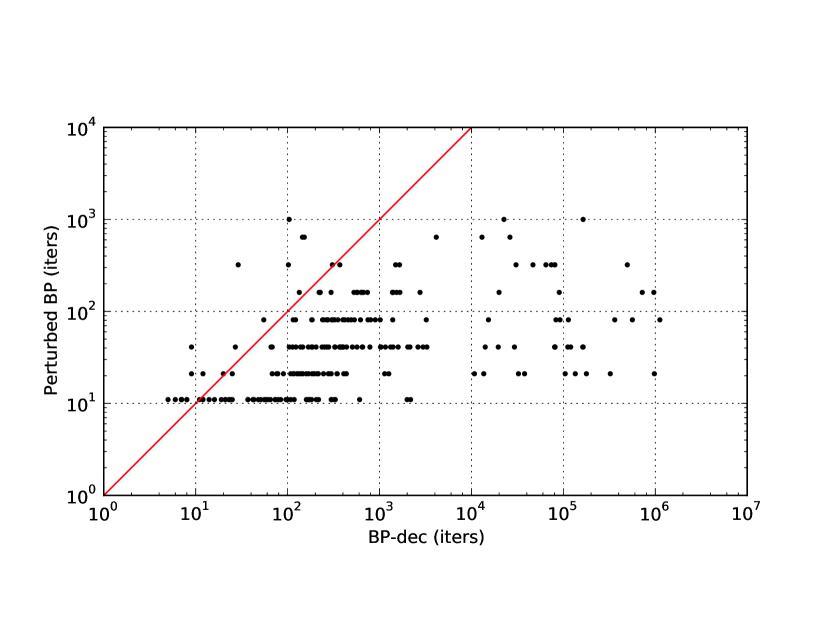
(a) iterations

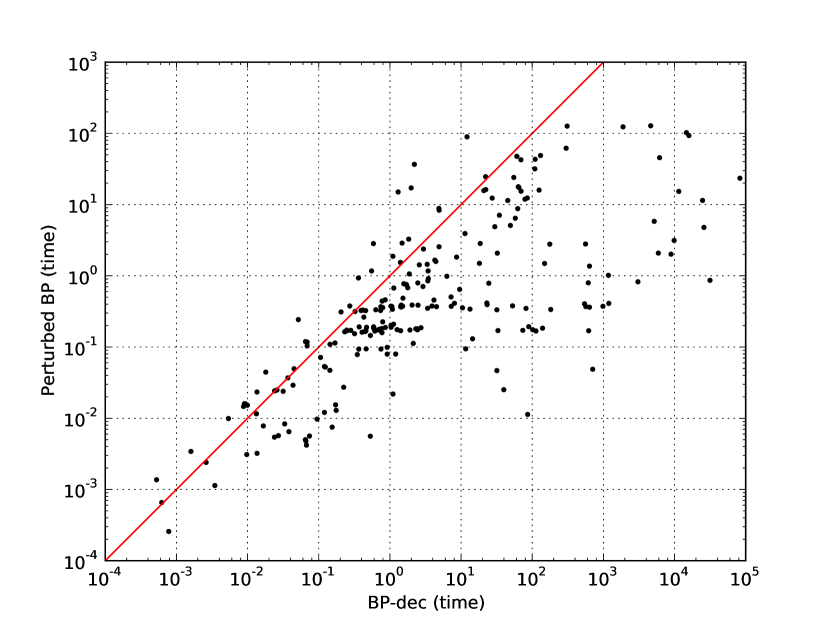
(b) time (seconds)

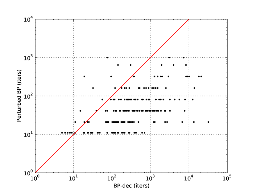
(c) iterations for $T=1000$

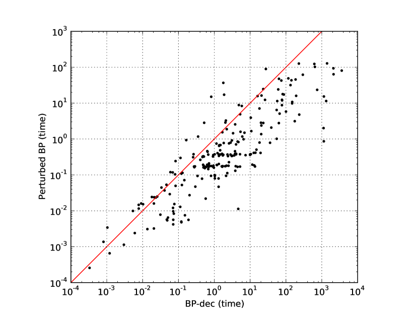
(d) time (seconds) for $T=1000$

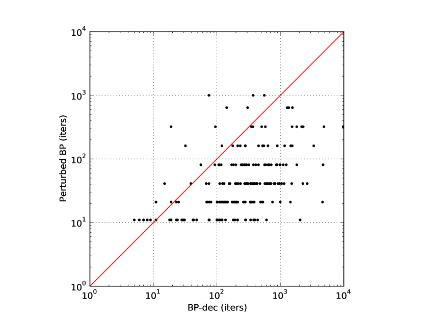
(e) iterations for $T=100$

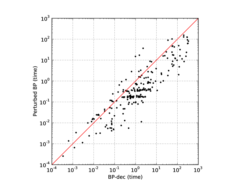
(f) time (seconds) for $T=100$

Figure 2: Comparison of time and number of iterations used by BP-dec and Perturbed BP in benchmark instances where both methods found satisfying assignments. (a,b) Maximum number of BP iterations per iteration of decimation is $T=10,240$, equal to the maximum iterations used by Perturbed BP. (c,d) Maximum number of iterations for BP in BP-dec is reduced to $T=1000$. (e,f) Maximum number of iterations for BP in BP-dec is further reduced to $T=100$.

Figure 2(a,b) compares the time and iterations of BP-dec and Perturbed BP for successful attempts where both methods satisfied an instance. The result for individual problem-sets is reported in the appendix.

Empirically, we found that Perturbed BP both solved (slightly) more instances than BP-dec (284 vs 253), and was (hundreds of times) more efficient: while Perturbed BP required only 133 iterations on average, BP-dec required an average of 41,284 iterations for successful instances.

We also ran BP-dec on all the benchmarks with maximum number of iterations set to $T=1000$ and $T=100$ iterations. This reduced the number of satisfied instances to $249$ for $T=1000$ and $247$ for $T=100$, but also reduced the average number of iterations to $1570$ and $562$ respectively, which are still several folds more expensive than Perturbed BP. Figure 2(c-f) compare the time and iterations used by BP-dec in these settings with that of Perturbed BP, when both methods found a satisfying assignment. See the appendix for a more detailed report on these results.

3 Critical Phenomena in Random CSPs

Random CSP (rCSP) instances have been extensively used in order to study the properties of combinatorial problems (Mitchell et al., 1992; Achioptas and Sorkin, 2000; Krzakala et al., 2007) as well as in analysis and design of algorithms (e.g.,  Selman et al., 1994; Mézard et al., 2002). Random CSPs are closely related to spin-glasses in statistical physics (Kirkpatrick and Selman, 1994; Fu and Anderson, 1986). This connection follows from the fact that the Hamiltonian of these spin-glass systems resembles the objective functions in many combinatorial problems, which decompose to pairwise (or higher order) interactions, allowing for a graphical representation in the form of a PGM. Here message passing methods, such as belief propagation (BP) and survey propagation (SP), provide consistency conditions on locally tree-like neighborhoods of the graph.

The analogy between a physical system and computational problem extends to their critical behavior where computation relates to dynamics (Ricci-Tersenghi, 2010). In computer science, this critical behavior is related to the time-complexity of algorithms employed to solve such problems, while in spin-glass theory this translates to dynamics of glassy state, and exponential relaxation times (Mézard et al., 1987). In fact, this connection has been used to attempt to prove the conjecture that $\mathcal{P}$ is not equal to $\mathcal{NP}$ (Deolalikar, 2010).

Studies of rCSP, as a critical phenomena, focus on the geometry of the solution space as a function of the problem’s difficulty, where rigorous (e.g.,  Achlioptas and Coja-Oghlan, 2008; Cocco et al., 2003) and non-rigorous (e.g., Cavity method of Mézard and Parisi (2001) and Mézard and Parisi (2003)) analyses have confirmed the same geometric picture.

When working with large random instances, a scalar $\alpha$ associated with a problem instance, a.k.a. control parameter – for example, the clause to variable ratio in SAT – can characterize that instance’s difficulty (i.e., larger control parameter corresponds to a more difficult instance) and in many situations it characterizes a sharp transition from satisfiability to unsatisfiability (Cheeseman et al., 1991).

Example 5 (Random $\kappa$-SAT)

Random $\kappa$-SAT instance with $N$ variables and $M=\alpha N$ constraints are generated by selecting $\kappa$ variables at random for each constraint. Each constraint is set to zero (i.e., unsatisfied) for a single random assignment (out of $2^{\kappa}$). Here $\alpha$ is the control parameter.

Example 6 (Random $q$-COL)

The control parameter for a random $q$-COL instances with $N$ variables and $M$ constraints is its average degree $\alpha=\frac{2M}{N}$. We consider Erdős-Rény random graphs and generate a random instance by sequentially selecting two distinct variables out of $N$ at random to generate each of $M$ edges. For large $N$, this is equivalent to selecting each possible factor with a fixed probability, which means the nodes have Poisson degree distribution $\mathbb{P}(|\partial i|=d)\propto e^{-\alpha}\alpha^{d}$.

While there are tight bounds for some problems (e.g.,  Achlioptas et al., 2005), finding the exact location of this transition for different CSPs is still an open problem. Besides transition to unsatisfiability, these analyses has revealed several other (phase) transitions (Krzakala et al., 2007). Figure 3(a)-(c) shows how the geometry of the set of solutions changes by increasing the control parameter.

Here we enumerate various phases of the problem for increasing values of the control parameter: (a) In the so-called Replica Symmetric (RS) phase, the symmetries of the set of solutions (a.k.a. ground states) reflect the trivial symmetries of problem w.r.t. variable domains. For example, for $q$-COL the set of solutions is symmetric w.r.t. swapping all red and blue assignment. In this regime, the set of solutions form a giant cluster (i.e., a set of neighboring solutions), where two solutions are considered neighbors when their Hamming distance is one (Achlioptas and Coja-Oghlan, 2008) or non-divergent with number of variables (Mézard and Parisi, 2003). Local search methods (e.g.,  Selman et al., 1994) and BP-dec can often efficiently solve random CSPs that belong to this phase.

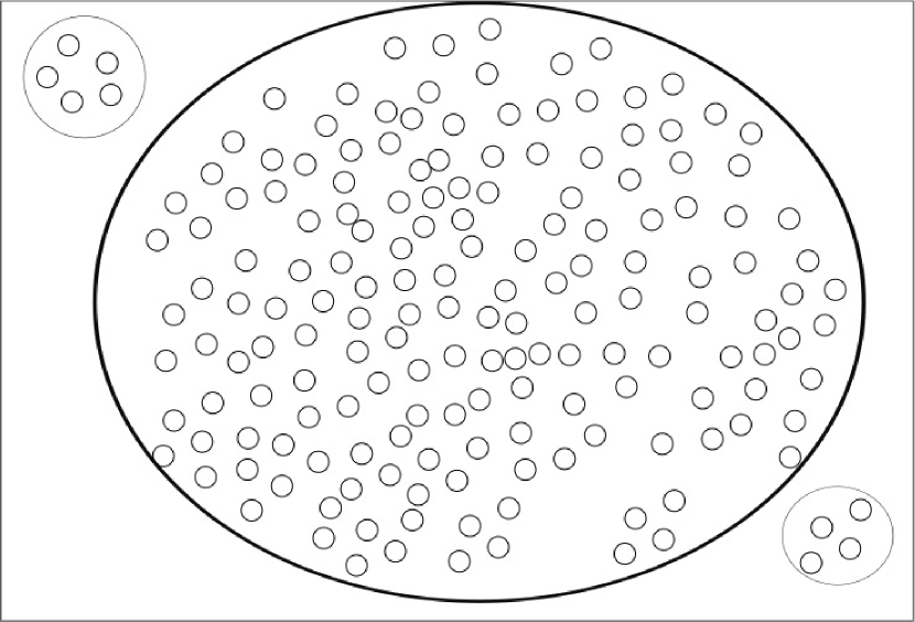
(a) Replica Symmetric

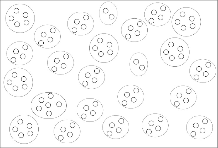
(b) clustering

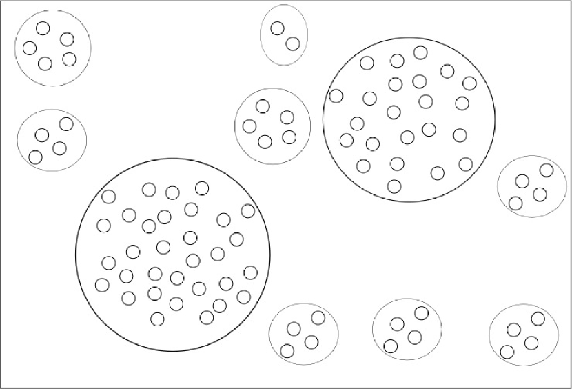
(c) condensation

Figure 3: A 2-dimensional schematic view of how the set of solutions of CSP varies as we increase the control parameter $\alpha$ from (a) replica symmetric phase to (b) clustering phase to (c) condensation phase. Here small circles represent solutions and the bigger circles represent clusters of solutions. Note that this view is very simplistic in many ways; for example, the total number of solutions and the size of clusters should generally decrease from (a) to (c).

(b) In clustering or dynamical transition (1dRSB), the set of solutions decomposes into an exponential number of distant clusters. Here two clusters are distant if the Hamming distance between their respective members is divergent (e.g., linear) in the number of variables. (c) In the condensation phase transition (1sRSB), the set of solutions condenses into a few dominant clusters. Dominant clusters have roughly the same number of solutions and they collectively contain almost all of the solutions. While SP can be used even within the condensation phase, BP usually fails to converge in this regime. However each cluster of solutions in the clustering and condensation phase is a valid fixed-point of BP, which is called a “quasi-solution” of BP. (d) A rigidity transition (not included in Figure 3) identifies a phase in which a finite portion of variables are fixed within dominant clusters. This transition triggers an exponential decrease in the total number of solutions, which leads to (e) unsatisfiability transition. This rough picture summarizes first order Replica Symmetry Breaking’s (1RSB) basic assumptions (Mézard and Montanari, 2009).

From a geometric perspective, the intuitive idea behind Perturbed BP, is to perturb the messages towards a solution. However, in order to achieve this, we need to initialize the messages to a proper neighborhood of a solution. Since these neighborhoods are not initially known, we resort to stochastic perturbation of messages to make local marginals more biased towards a subspace of solutions. This continuous perturbation of all messages is performed in a way that allows each BP message to re-adjust itself to the other perturbations, more and more focusing on a random subset of solutions.

3.1 1RSB Postulate and Survey Propagation

Large random graphs are locally tree-like, which means the length of short loops are typically in the order of $\log(N)$ (Janson et al., 2001). This ensures that, in the absence of long-range correlations, BP is asymptotically exact, as the set of messages incoming to each node or factor are almost independent. Although BP messages remain uncorrelated until the condensation transition (Krzakala et al., 2007), the BP equations do not completely characterize the set of solutions after the clustering transition. This inadequacy is indicated by the existence of a set of several valid fixed points (rather than a unique fixed-point) for BP, each of which corresponds to a quasi-solution. For a better intuition, consider the cartoons of Figures 3(b) and (c). During the clustering phase (b), $x_{i}$ and $x_{j}$ (corresponding to the $x$ and $y$ axes) are not highly correlated, but they become correlated during and after condensation (c). This correlation between variables that are far apart in the PGM results in correlation between the BP messages. This violates BP’s assumption that messages are uncorrelated, which results in BP’s failure in this regime.

1RSB’s approach to incorporating this clustering of solutions into the equilibrium conditions is to define a new Gibbs measure over clusters. Let $\mathbf{y}\subset\mathcal{S}$ denote a cluster of solutions and $\mathcal{Y}$ be the set of all such clusters. The idea is to treat $\mathcal{Y}$ the same as we treated $\mathcal{X}$, by defining a distribution

$$\boldsymbol{\mu}(\mathbf{y})\quad\propto\quad{|\mathbf{y}|^{m}}\quad\forall\;\mathbf{y}\in\mathcal{Y}$$ (16)

where ${m}\in[0,1]$, called the Parisi parameter (Mézard et al., 1987), specifies how each cluster’s weight depends on its size. This implicitly defines a distribution over $\mathcal{X}$

$$\mu(x)\quad\propto\quad\sum_{\mathbf{y}\ni x}\boldsymbol{\mu}(\mathbf{y})$$ (17)

N.b., ${m}=1$ corresponds to the original distribution (Eq 1).

Example 7

Going back to our simple 3-SAT example, $\mathbf{y}^{(1)}=\{(True,True,True)\}$ and $\mathbf{y}^{(2)}=\{(False,False,False),\ (False,False,True)\}$ are two clusters of solutions. Using $m=1$, we have
$\boldsymbol{\mu}(\{\{True,True,True\}\})=1/3$ and $\boldsymbol{\mu}(\{\{False,False,False\},\{False,False,True\}\})=2/3$. This distribution over clusters reproduces the distribution over solutions – i.e., $\mu(x)=1/3\;\forall x\in\mathcal{S}$. On the other hand, using $m=0$, produces a uniform distribution over clusters, but it does not give us a uniform distribution over the solutions.

This meta-construction for $\mu(\mathbf{y})$ can be represented using an auxiliary PGM. One may use BP to find marginals over this PGM; here BP messages are distributions over all BP messages in the original PGM, as each cluster is a fixed-point for BP. This requirement to represent a distribution over distributions makes 1RSB practically intractable. In general, each original BP message is a distribution over $\mathcal{X}_{i}$ and it is difficult to define a distribution over this infinite set. However this simplifies if the original BP messages can have limited values. Fortunately if we apply max-product BP to solve a CSP, instead of sum-product BP (of Eqs 3 and 4), the messages can have a finite set of values.

Max-Product BP: Our previous formulation of CSP was using sum-product BP. In general, max-product BP is used to find the Maximum a Posteriori (MAP) assignment in a PGM, which is a single assignment with the highest probability. In our PGM, the MAP assignment is a solution for the CSP. The max-product update equations are

$$\eta_{i\to{I}}(x_{i})\;=\;\prod_{J\in\partial i\setminus I}\eta_{J\to i}(x_{i})\; =\;{\Lambda}_{i\to I}(\ \{\eta_{J\to i}\}_{J\in\partial i\setminus I}\ )(x_{i})$$ (18)

$$\eta_{I\to i}(x_{i})\;=\;\max_{\mathcal{X}_{\partial I\setminus i}}C_{I}(x_{I})\prod_{j\in\partial I\setminus i}\eta_{j\to I}(x_{j})\; =\;{\Lambda}_{I\to i}(\ \{\eta_{j\to I}\}_{j\in\partial I\setminus i}\ )(x_{i})$$ (19)

$$\widehat{\mu}(x_{i})\;=\;\prod_{J\in\partial i}\eta_{J\to i}(x_{i})\; =\;{\Lambda}_{i}(\ \{\eta_{J\to i}\}_{J\in\partial i}\ )(x_{i})$$ (20)

where ${\Lambda}=\{{\Lambda}_{i\to I},{\Lambda}_{I\to i}\}_{i,I\in\partial I}$ is the max-product BP operator and ${\Lambda}_{i}$ represents the marginal estimate as a function of messages. Note that here messages and marginals are not distributions. We initialize $\nu_{i\to I}(x_{i})\in\{0,1\},\;\forall I,i\in\partial I,x_{i}\in\mathcal{X}_{i}$. Because of the way constraints and update equations are defined, at any point during the updates we have $\nu_{i\to I}(x_{i})\in\{0,1\}$. This is also true for $\widehat{\mu}(x_{i})$. Here any of $\nu_{i\to I}(x_{i})=1$, $\nu_{I\to i}(x_{i})=1$ or $\widehat{\mu}(x_{i})=1$, shows that value $x_{i}$ is allowed according to a message or marginal, while $0$ forbids that value. Note that $\widehat{\mu}(x_{i})={0}\;\forall x_{i}\in\mathcal{X}_{i}$ iff no solution was found, because the incoming messages were contradictory. The non-trivial fixed-points of max-product BP define quasi-solutions in 1RSB phase, and therefore define clusters $\mathbf{y}$.

Example 8

If we initialize all messages to $1$ for our simple 3-SAT example, the final marginals over all the variables are equal to 1, allowing all assignments for all variables. However beside this trivial fixed-point, there are other fixed points that correspond to two clusters of solutions.

For example, considering the cluster $\{(False,False,False),(False,False,True)\}$, the following $\{\eta_{i\to I}\}$ (and their corresponding $\{\eta_{I\to i}\}$ define a fixed-point for max-product BP:

$$\eta_{1\to I}(True)=\widehat{\mu}_{1}(True)=0 \quad\eta_{1\to I}(False)=\widehat{\mu}_{1}(False)=1\quad \forall I\in\partial 1$$

$$\eta_{2\to I}(True)=\widehat{\mu}_{2}(True)=0 \quad\eta_{2\to I}(False)=\widehat{\mu}_{2}(False)=1\quad \forall I\in\partial 2$$

$$\eta_{3\to I}(True)=\widehat{\mu}_{3}(True)=1 \quad\quad\eta_{3\to I}(False)=\widehat{\mu}_{3}(False)=1\quad \forall I\in\partial 3$$

Here the messages indicate the allowed assignments within this particular cluster of solutions.

3.1.1 Survey Propagation

Here we define the 1RSB update equations over max-product BP messages. We skip the explicit construction of the auxiliary PGM that results in SP update equations, and confine this section to the intuition offered by SP messages. For the construction of the auxiliary-PGM see (Braunstein and Zecchina, 2003) and (Mézard and Montanari, 2009). See (Maneva et al., 2007) for a different perspective on the relation of BP and SP for the satisfiability problem and (Kroc et al., 2007) for an experimental study of SP applied to SAT.

Let $\mathcal{Y}_{i}=2^{|\mathcal{X}_{i}|}$ be the power-set of $\mathcal{X}_{i}$. Each max-product BP message can be seen as a subset of $\mathcal{X}_{i}$ that contains the allowed states. Therefore $\mathcal{Y}_{i}$ as its power-set contains all possible max-product BP messages. Each message $\boldsymbol{\nu}_{i\to I}:\;\mathcal{Y}_{i}\to[0,1]$ in the auxiliary PGM defines a distribution over original max-product BP messages.

Example 9 (3-COL)

$\mathcal{X}_{i}=\{1,2,3\}$ is the set of colors and
$\mathcal{Y}_{i}=\{\{\},\{1\},\{2\},\{3\},\{1,2\},\{2,3\},\{1,3\},\{1,2,3\}\}$. Here $\mathbf{y}_{i}=\{\}$ corresponds to the case where none of the colors are allowed.

Applying sum-product BP to our auxiliary PGM gives entropic SP(${m}$) updates as:

$$\boldsymbol{\nu}_{i\to I}(\mathbf{y}_{i})\propto|\mathbf{y}_{i}|^{{m}}\;\sum_{\{\eta_{J\to i}\}_{J\in\partial i\setminus I}}\delta(\mathbf{y}_{i},{\Lambda}_{i\to I}(\{\eta_{J\to i}\}_{J\in\partial i\setminus I}))\prod_{J\in\partial i\setminus I}\boldsymbol{\nu}_{J\to i}(\eta_{J\to i})$$ (21)

$$\boldsymbol{\nu}_{I\to i}(\mathbf{y}_{i})\propto|\mathbf{y}_{i}|^{{m}}\;\sum_{\{\eta_{j\to I}\}_{j\in\partial I\setminus i}}\delta(\mathbf{y}_{i},{\Lambda}_{I\to i}(\{\eta_{j\to I}\}_{j\in\partial I\setminus i}))\prod_{j\in\partial I\setminus i}\boldsymbol{\nu}_{j\to I}(\eta_{j\to I})$$ (22)

$$\boldsymbol{\nu}_{i\to{I}}(\{\})\quad:=\quad\boldsymbol{\nu}_{I\to{i}}(\{\})\quad:=\quad 0\quad\quad\forall i,\;I\in\partial i$$ (23)

where the summations are over all combinations of max-product BP messages. Here the $\delta$-function ensures that only the set of incoming messages that satisfy the original BP equations make contributions. Since we only care about the valid assignments and $\mathbf{y}_{i}=\{\}$ forbids all assignments, we ignore its contribution (Eq 23).

Example 10 (3-SAT)

Consider the SP message $\boldsymbol{\nu}_{1\to C_{1}}(\mathbf{y}_{1})$ in the factor graph of Figure 1(b). Here the summation in Eq 21 is over all possible combinations of incoming max-product BP messages $\eta_{C_{2}\to 1},\ldots,\eta_{C_{5}\to 1}$. Since each of these messages can assume one of the three valid values – e.g., 
$\eta_{C^{2}\to 1}(x_{1})\in\{\ \{True\},\{False\},\{True,False\}\ \}$ – for each particular assignment of $\mathbf{y}_{1}$, a total of
$|\{\{True\},\{False\},\{True,False\}\}|^{|\partial 1\setminus C_{1}|}=3^{4}$ possible combinations are enumerated in the summations of Eq 21. However only the combinations that form a valid max-product message update have non-zero contribution in calculating $\boldsymbol{\nu}_{1\to C_{1}}(\mathbf{y}_{1})$. These are basically the messages that appear in a max-product fixed point as discussed in Example 8.

Each of original messages corresponds to a different sub-set of clusters and ${m}$ (from Eq 16) controls the effect of each cluster’s size on its contribution. At any point, we can use these messages to estimate the marginals of $\widehat{\boldsymbol{\mu}}(\mathbf{y})$ defined in Eq 16

$$\widehat{\boldsymbol{\mu}}(\mathbf{y}_{i})\;\propto\;|\mathbf{y}_{i}|^{{m}}\;\sum_{\{\eta_{J\to i}\}_{J\in\partial i}}\delta(\mathbf{y}_{i},\ {\Lambda}_{i}(\ \{\eta_{J\to i}\}_{J\in\partial i})\ )\prod_{J\in\partial i}\boldsymbol{\nu}_{J\to i}(\eta_{J\to i})$$ (24)

This also implies a distribution over the original domain, which we slightly abuse notation to denote by:

$$\widehat{\boldsymbol{\mu}}(x_{i})\;\propto\;\sum_{\mathbf{y}_{i}\ni x_{i}}\widehat{\boldsymbol{\mu}}(\mathbf{y}_{i})$$ (25)

The term SP usually refers to SP($0$) – i.e., $m=0$ – where all clusters, regardless of their size, contribute the same amount to $\boldsymbol{\mu}(\mathbf{y})$. Now that we can obtain an estimate of marginals, we can employ this procedure within a decimation process to incrementally fix some variables. Here either $\widehat{\boldsymbol{\mu}}(x_{i})$ or $\widehat{\boldsymbol{\mu}}(\mathbf{y}_{i})$ can be used by the decimation procedure to fix the most biased variables. In the former case, a variable $\mathbf{y}_{i}$ is fixed to $\mathbf{y}_{i}^{*}=\{x^{*}_{i}\}$ when $x^{*}_{i}=\arg_{x_{i}}\max\widehat{\boldsymbol{\mu}}(x_{i})$. In the latter case, $\mathbf{y}_{i}^{*}=\arg_{y_{i}}\max\widehat{\boldsymbol{\mu}}(\mathbf{y}_{i})$. Here we use SP-dec(S) to refer to the former procedure (that uses $\widehat{\boldsymbol{\mu}}(x_{i})$ to fix variables to a single value) and use SP-dec(C) to refer to the later case (in which variables are fixed to a cluster of assignments).

The original decimation procedure for $\kappa$-SAT (Braunstein et al., 2002) corresponds to SP-dec(S). SP-dec(C) for CSP with Boolean variables is only slightly different, as SP-dec(C) can choose to fix a cluster to $\mathbf{y}_{i}=\{True,False\}$ in addition to the options of $\mathbf{y}_{i}=\{True\}$ and $\mathbf{y}_{i}=\{False\}$, available to SP-dec(S). However, for larger domains (e.g., $q$-COL), SP-dec(C) has a clear advantage. For example in $3$-COL, SP-dec(C) may choose to fix a cluster to $\mathbf{y}_{i}=\{1,2\}$ while SP-dec(S) can only choose between $\mathbf{y}_{i}\in\{\{1\},\{2\},\{3\}\}$. This significant difference is also reflected in their comparative success-rate on $q$-COL. (See Table 1 in Section 3.3.)

During the decimation process, usually after fixing a subset of variables, the SP marginals $\widehat{\boldsymbol{\mu}}(x_{i})$ become uniform, indicating that clusters of solutions have no preference over particular assignments of the remaining variables. The same happens when we apply SP to random instances in RS phase. At this point (a.k.a. paramagnetic phase), a local search method or BP-dec can often efficiently find an assignment to the variables that are not yet fixed by decimation. Note that both SP-dec(C) and SP-dec(S) switch to local search as soon as all $\widehat{\boldsymbol{\mu}}(x_{i})$ become close to uniform.

The computational complexity of each SP update of Eq 22 is $\mathcal{O}(2^{|\mathcal{X}_{i}|}-1)^{|\partial I|}$ as for each particular value $\mathbf{y}_{i}$, SP needs to consider every combination of incoming messages, each of which can take $2^{|\mathcal{X}_{i}|}$ values (minus the empty set). Similarly, using a naive approach the cost of update of Eq 21 is $\mathcal{O}(2^{|\mathcal{X}_{i}|}-1)^{|\partial i|}$. However by considering incoming messages one at a time, we can perform the same exact update in $\mathcal{O}(|\partial i|\;2^{2|\mathcal{X}_{i}|})$. In comparison to the cost of BP updates, we see that SP updates are substantially more expensive for large $|\mathcal{X}_{i}|$ and $|\partial I|$.

3.2 Perturbed Survey Propagation

The perturbation scheme that we use for SP is similar to what we did for BP. Let
$\boldsymbol{\Phi}_{i\to I}(\ \{\boldsymbol{\nu}_{j\to J}\}_{j\in\Delta i,(J\in\partial i)\setminus I})\ )$ denote the update operator for the message from variable $\mathbf{y}_{i}$ to factor $C_{I}$. This operator is obtained by substituting Eq 22 into Eq 21 to get a single SP update equation. Let $\boldsymbol{\Phi}(\{\boldsymbol{\nu}_{i\to I}\}_{i,I\in\partial i})$ denote the aggregate SP operator, which applies $\boldsymbol{\Phi}_{i\to I}$ to update each individual message.

We perform Gibbs sampling from the “original” domain $\mathcal{X}$ using the implicit marginal of Eq 25. We denote this random operator by $\boldsymbol{\Psi}=\{\boldsymbol{\Psi}_{i}\}_{i}$:

$$\boldsymbol{\nu}_{i\to I}(\mathbf{y}_{i})\;=\;\boldsymbol{\Psi}_{i}(\ \{\boldsymbol{\nu}_{j\to J}\}_{j\in\Delta i,J\in\partial i}\ )\;\triangleq\;\delta(\mathbf{y}_{i},\{\widehat{x}_{i}\})\quad\text{where}\;\widehat{x}_{i}\sim\widehat{\boldsymbol{\mu}}(x_{i})$$ (26)

where the second argument of the $\delta$-function is a singleton set, containing a sample from the estimate of marginal.

Now, define the Perturbed SP operator as the convex combination of SP and either of the GS operator above:

$$\boldsymbol{\Gamma}(\{\boldsymbol{\nu}_{i\to I}\})\;\triangleq\;\gamma\boldsymbol{\Psi}(\{\boldsymbol{\nu}_{i\to I}\})\;+\;(1-\gamma)\boldsymbol{\Phi}(\{\boldsymbol{\nu}_{i\to I}\})$$ (27)

Similar to perturbed BP, during iterations of Perturbed SP, $\gamma$ is gradually increased from $0$ to $1$. If perturbed SP reaches the final iteration, the samples from the implicit marginals represent a satisfying assignment. The advantage of this scheme to SP-dec is that perturbed SP does not require any further local search. In fact we may apply $\boldsymbol{\Gamma}$ to CSP instances in the RS phase as well, where the solutions form a single giant cluster. In contrast, applying SP-dec, to these instances simply invokes the local search method.

To demonstrate this, we applied Perturbed SP(S) to benchmark CSP instances of Table 2 in which the maximum number of elements in the factor was less than $10$. Here Perturbed SP(S) solved $80$ instances out of $202$ cases, while Perturbed BP solved $78$ instances.

3.3 Experiments on random CSP

We implemented all the methods above for general factored CSP using the libdai code base (Mooij, 2010). To our knowledge this is the first general implementation of SP and SP-dec. Previous applications of SP-dec to $\kappa$-SAT and $q$-COL (Braunstein et al., 2003; Mulet et al., 2002; Braunstein et al., 2002) were specifically tailored to just one of those problems.

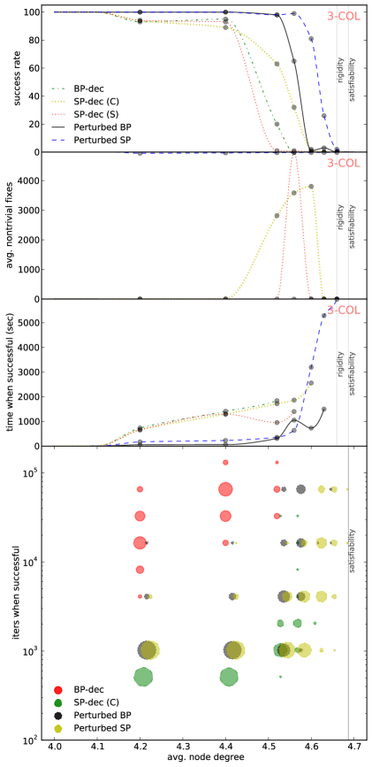
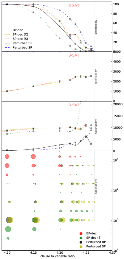
Figure 4: (first row) Success-rate of different methods for 3-COL and 3-SAT for various control parameters. (second row) The average number of variables (out of $N=5000$) that are fixed using SP-dec (C) and (S) before calling local search, averaged over 100 instances. (third row) The average amount of time (in seconds) used by the successful setting of each method to find a satisfying solution. For SP-dec(C) and (S) this includes the time used by local search. (fourth row) The number of iterations used by different methods at different control parameters, when the method was successful at finding a solution. The number of iterations for each of 100 random instances is rounded to the closest power of 2. This does not include the iterations used by local search after SP-dec.

Here we report the results on $\kappa$-SAT for $\kappa\in\{3,4\}$ and $q$-COL for $q\in\{3,4,9\}$. We used the procedure discussed in the examples of Section 3 to produce $100$ random instances with $N=5,000$ variables for each control parameter $\alpha$. We report the probability of finding a satisfying assignment for different methods (i.e., the portion of $100$ instances that were satisfied by each method). For coloring instances, to help decimation, we break the initial symmetry of the problem by fixing a single variable to an arbitrary value.

For BP-dec and SP-dec, we use a convergence threshold of $\epsilon=.001$ and fix $\rho=1\%$ of variables per iteration of decimation. Perturbed BP and Perturbed SP use $T=1000$ iterations. Decimation-based methods use a maximum of $T=1000$ iterations per iteration of decimation. If any of the methods failed to find a solution in the first attempt, $T$ was increased by a factor of $4$ at most $3$ times (so in the final attempt: $T=64,000$). To avoid blow-up in run-time, for BP-dec and SP-dec, only the maximum iteration, $T$, during the first iteration of decimation, was increased (this is similar to the setting of Braunstein et al. (2002) for SP-dec). For both variations of SP-dec (see Section 3.1.1), after each decimation step, if $\max_{i,x_{i}}\mu(x_{i})-\frac{1}{|\mathcal{X}_{i}|}<.01$ we consider the instance para-magnetic, and run BP-dec (with $T=1000$, $\epsilon=.001$ and $\rho=1\%$) on the simplified instance.

Figure 4(first row) visualizes the success rate of different methods on $100$ instances of 3-SAT (right) and 3-COL (left). Figure 4(second row) reports the number of variables that are fixed by SP-dec(C) and (S) before calling BP-dec as local search. The third row shows the average amount of time that is used to find a satisfying solution. This does not include the failed attempts. For SP-dec variations, this time includes the time used by local search. The final row of Figure 4 shows the number of iterations used by each method at each level of difficulty over the successful instances. Here the area of each disk is proportional to the frequency of satisfied instances with that particular number of iterations for each control parameter and inference method.

Here we make the following observations:

• Perturbed BP is much more effective than BP-dec, while remaining ten to hundreds of times more efficient.

• As the control parameter grows larger, the chance of requiring more iterations to satisfy the instance increases for all methods.

• Although computationally very inefficient, BP-dec is able to find solutions for instances with larger control parameters than suggested by previous results (e.g.,  Mézard and Montanari, 2009).

• For many instances where SP-dec(C) and (S) use few iterations, the variables are fixed to a trivial cluster $\mathbf{y}_{i}=\mathcal{X}_{i}$, which allows all assignments. This is particularly pronounced for 3-COL, where up to $\alpha=4.4$ the non-trivial fixes remains zero and therefore the success rate up to this point is solely due to BP-dec.

• While for 3-SAT, SP-dec(C) and SP-dec(S) have a similar performance, for 3-COL, SP-dec(C) significantly outperforms SP-dec(S).

Table 1 reports the success-rate as well as the average of total iterations in the successful attempts of each method. Here the number of iterations for SP-dec(C) and (S) is the sum of iterations used by the method and the following local search. We observe that Perturbed BP can solve most of the easier instances using only $T=1000$ iterations (e.g., see Perturb BP’s result for 3-SAT at $\alpha=4.1$, 3-COL at $\alpha=4.2$ and 9-COL at $\alpha=33.4$).

Table 1 also supports our speculation in Section 3.1.1 that SP-dec(C) is in general preferable to SP-dec(S), in particular when applied to the coloring problem.

The most important advantage of Perturbed BP over SP-dec and Perturbed SP is that Perturbed BP can be applied to instances with large factor cardinality (e.g., $10$-SAT) and large variable domains (e.g., $9$-COL). For example for $9$-COL, the cardinality of each SP message is $2^{9}=512$, which makes SP-dec and Perturbed SP impractical. Here BP-dec is not even able to solve a single instance around the dynamical transition (as low as $\alpha=33.4$) while Perturbed BP satisfies all instances up to $\alpha=34.1$. Besides the experimental results reported here, we have also used perturbed BP to efficiently solve other CSPs such as K-Packing, K-set-cover and clique-cover within the context of min-max inference (Ravanbakhsh et al., 2014).

Table 1: Comparison of different methods on $\{3,4\}$-SAT and $\{3,4,9\}$-COL. For each method the success-rate and the average number of iterations (including local search) on successful attempts are reported. The approximate location of phase transitions are from (Montanari et al., 2008; Zdeborova and Krzakala, 2007) .

3.4 Discussion

It is easy to check that, for ${m}=1$, SP updates produce sum-product BP messages as an average case; that is, the SP updates (Eqs 21 and 22) reduce to that of sum-product BP (Eqs 3 and 4) where

$$\nu_{i\to{I}}(x_{i})\quad\propto\sum_{\mathbf{y}_{i}\ni x_{i}}\boldsymbol{\nu}_{i\to{I}}(\mathbf{y}_{i})$$ (28)

Figure 5: This schematic view demonstrates the clustering during condensation phase. Here assume $x$ and $y$ axes correspond to $x_{1}$ and $x_{2}$. Considering the whole space of assignments, $x_{1}$ and $x_{2}$ are highly correlated. The formation of this correlation between distant variables on a PGM breaks BP. Now assume that Perturbed BP messages are focused on the largest shaded ellipse. In this case the correlation is significantly reduced.

This suggests that the BP equation remains correct wherever SP($1$) holds, which has lead to the belief that BP-dec should perform well up to the condensation transition (Krzakala et al., 2007). However in reaching this conclusion, the effect of decimation was ignored. More recent analyses (Coja-Oghlan, 2011; Montanari et al., 2007; Ricci-Tersenghi and Semerjian, 2009) draw a similar conclusion about the effect of decimation: At some point during the decimation process, variables form long-range correlations such that fixing one variable may imply an assignment for a portion of variables that form a loop, potentially leading to contradictions. Alternatively the same long-range correlations result in BP’s lack of convergence and error in marginals that may lead to unsatisfying assignments.

Perturbed BP avoids the pitfalls of BP-dec in two ways: (I) Since many configurations have non-zero probability until the final iteration, Perturbed BP can avoid contradictions by adapting to the most recent choices. This is in contrast to decimation in which variables are fixed once and are unable to change afterwards. A backtracking scheme suggested by Parisi (2003) attempts to fix the same problem with SP-dec. (II) We speculate that simultaneous bias of all messages towards sub-regions over which the BP equations remain valid, prevents the formation of long-range correlations between variables that breaks BP in 1sRSB; see Figure 5.

In all experiments, we observed that Perturbed BP is competitive with SP-dec, while BP-dec often fails on much easier problems. We saw that the cost of each SP update grows exponentially faster than the cost of each BP update. Meanwhile, our perturbation scheme adds a negligible cost to that of BP – i.e., that of sampling from these local marginals and updating the outgoing messages accordingly. Considering the computational complexity of SP-dec, and also the limited setting under which it is applicable, Perturbed BP is an attractive substitute. Furthermore our experimental results also suggest that Perturbed SP(S) is a viable option for real-world CSPs with small variable domains and constraint cardinalities.

Conclusion

We considered the challenge of efficiently producing assignments that satisfy hard combinatorial problems, such as $\kappa$-SAT and $q$-COL. We focused on ways to use message passing methods to solve CSPs, and introduced a novel approach, Perturbed BP, that combines BP and GS in order to sample from the set of solutions. We demonstrated that Perturbed BP is significantly more efficient and successful than BP-dec. We also demonstrated that Perturbed BP can be as powerful as a state-of-the-art algorithm (SP-dec), in solving rCSPs while remaining tractable for problems with large variable domains and factor cardinalities. Furthermore we provided a method to apply the similar perturbation procedure to SP, producing the Perturbed SP process that outperforms SP-dec in solving difficult rCSPs.

A. Detailed Results for Benchmark CSP

In Table 2 we report the average number of iterations and average time for the attempt that successfully found a satisfying assignment (i.e., the failed instances are not included in the average). We also report the number of satisfied instances for each method as well as the number of satisfiable instance in that series of problems (if known). Further information about each data-set maybe obtained from Lecoutre (2013).

Table 2: Comparison of Perturbed BP and BP-guided decimation on benchmark CSPs.

				BP-dec			Perturbed BP
problem	series	instances	$\#$ satisfiable	$\#$ satisfied	avg. time (s)	avg. iters	$\#$ satisfied	avg. time (s)	avg. iters
Geometric	-	100	92	77	208.63	30383	81	.70	74
Dimacs	aim-50	24	16	9	11.41	25344	14	.07	181
	aim-100	24	16	8	18.2	16755	11	.15	213
	aim-200	24	N/A	7	401.90	160884	6	.17	46
	ssa	8	N/A	4	.60	373.25	4	.50	86
	jhnSat	16	16	16	5839.86	141852	13	9.82	117
	varDimacs	9	N/A	4	2.95	715	4	.12	18
QCP	QCP-10	15	10	10	43.87	30054	10	.22	51
	QCP-15	15	10	3	5659.70	600741	4	9.59	530
	QCP-25	15	10	0	0	0	0	0	0
Graph-Coloring	ColoringExt	17	N/A	4	.05	103	5	.04	25
	school	8	N/A	0	N/A	N/A	5	62.86	153
	myciel	16	N/A	5	.21	59	5	.05	11
	hos	13	N/A	5	27.34	606	5	10.04	37
	mug	8	N/A	4	.068	313	4	.004	11
	register-fpsol	25	N/A	0	N/A	N/A	0	N/A	N/A
	register-inithx	25	N/A	0	N/A	N/A	0	N/A	N/A
	register-zeroin	14	N/A	3	5906.16	26544	0	N/A	N/A
	register-mulsol	49	N/A	5	59.27	418	0	N/A	N/A
	sgb-queen	50	N/A	7	35.66	916	11	7.56	81
	sgb-games	4	N/A	1	.91	434	1	.07	21
	sgb-miles	34	N/A	4	20.86	371	2	4.20	181
	sgb-book	26	N/A	5	1.72	444	5	.18	39
	leighton-5	8	N/A	0	N/A	N/A	0	N/A	N/A
	leighton-15	28	N/A	0	N/A	N/A	1	106.46	641
	leighton-25	29	N/A	2	304.49	1516	2	94.11	241
All Interval Series	series	12	12	2	4.78	11319	7	1.85	520
Job Shop	e0ddr1	10	10	9	707.74	9195	5	37	257
	e0ddr2	10	10	5	3640.40	26544	7	74.49	366
	ewddr2	10	10	10	10871.96	48053	9	21.24	72
Schurr’s Lemma	-	10	N/A	1	39.89	120152	2	.97	100
Ramsey	Ramsey 3	8	N/A	1	.01	61	4	.75	283
	Ramsey 4	8	N/A	2	12941.51	561300	7	7.39	81
Chessboard Coloration	-	14	N/A	5	35.51	3111	5	.66	27
Hanoi	-	3	3	3	.48	12	3	.52	14
Golomb Ruler	Arity 3	8	N/A	2	1.39	103	2	19.78	660
Queens	queens	8	8	7	3.30	159	8	2.43	57
Multi-Knapsack	mknap	2	2	2	2.44	6	2	4.41	10
Driver	-	7	7	5	10.14	1438	5	4.74	274
Composed	25-10-20	10	10	8	1.62	695	5	.17	38
Langford	lagford-ext	4	2	0	N/A	N/A	1	.002	10
	lagford 2	22	N/A	4	.67	127	10	11.64	10
	lagford 3	20	N/A	0	N/A	N/A	N/A	N/A	N/A

References

- Achioptas and Sorkin (2000) D Achioptas and Gregory B Sorkin. Optimal myopic algorithms for random 3-sat. In Foundations of Computer Science, 2000. Proceedings. 41st Annual Symposium on, pages 590–600. IEEE, 2000.
- Achlioptas and Coja-Oghlan (2008) D Achlioptas and A Coja-Oghlan. Algorithmic barriers from phase transitions. arXiv:0803.2122, March 2008.
- Achlioptas et al. (2005) D Achlioptas, A Naor, and Y Peres. Rigorous location of phase transitions in hard optimization problems. Nature, 435(7043):759–764, June 2005. ISSN 0028-0836. doi: 10.1038/nature03602.
- Andrieu et al. (2003) C Andrieu, N de Freitas, A Doucet, and M Jordan. An introduction to MCMC for machine learning. Machine Learning, 2003.
- Braunstein and Zecchina (2003) A Braunstein and R Zecchina. Survey propagation as local equilibrium equations. CoRR, 2003.
- Braunstein et al. (2002) A Braunstein, M Mézard, and R Zecchina. Survey propagation: an algorithm for satisfiability. Random Structures and Algorithms, 27(2):19, 2002.
- Braunstein et al. (2003) A Braunstein, R Mulet, A Pagnani, M Weigt, and R Zecchina. Polynomial iterative algorithms for coloring and analyzing random graphs. Physical Review E, 68(3):036702, 2003.
- Cheeseman et al. (1991) P Cheeseman, B Kanefsky, and W M Taylor. Where the really hard problems are. In Proceedings of the 12th IJCAI - Volume 1, IJCAI’91, pages 331–337, San Francisco, CA, USA, 1991. Morgan Kaufmann Publishers Inc. ISBN 1-55860-160-0.
- Cocco et al. (2003) S Cocco, O Dubois, J Mandler, and R Monasson. Rigorous decimation-based construction of ground pure states for spin-glass models on random lattices. Physical review letters, 90(4):047205, 2003.
- Coja-Oghlan (2011) A Coja-Oghlan. On belief propagation guided decimation for random k-sat. In Proceedings of the Twenty-Second Annual ACM-SIAM Symposium on Discrete Algorithms, SODA ’11, pages 957–966. SIAM, 2011.
- Deolalikar (2010) V. Deolalikar. Deolalikar P vs NP paper, 2010. URL {http://michaelnielsen.org/polymath1/index.php?title=Deolalikar_P_vs_NP_paper}.
- Fu and Anderson (1986) Y Fu and P W Anderson. Application of statistical mechanics to NP-complete problems in combinatorial optimisation. Journal of Physics A: Mathematical and General, 19(9):1605–1620, June 1986. ISSN 0305-4470, 1361-6447. doi: 10.1088/0305-4470/19/9/033.
- Garey and Johnson (1979) M R Garey and D S Johnson. Computers and Intractability: A Guide to the Theory of NP-Completeness, volume 44 of A Series of Books in the Mathematical Sciences. W. H. Freeman, 1979. ISBN 0716710455.
- Ihler and Mcallester (2009) A T Ihler and D A Mcallester. Particle belief propagation. In International Conference on Artificial Intelligence and Statistics, pages 256–263, 2009.
- Janson et al. (2001) S Janson, T Luczak, and V. F. Kolchin. Random graphs. Bull. London Math. Soc, 33:363–383, 2001.
- Kask et al. (2004) K Kask, R Dechter, and V Gogate. Counting-based look-ahead schemes for constraint satisfaction. In Principles and Practice of Constraint Programming–CP 2004, pages 317–331. Springer, 2004.
- Kautz et al. (2009) H A. Kautz, A Sabharwal, and B Selman. Incomplete algorithms. In Armin Biere, Marijn Heule, Hans van Maaren, and Toby Walsh, editors, Handbook of Satisfiability, volume 185 of Frontiers in Artificial Intelligence and Applications, pages 185–203. IOS Press, 2009. ISBN 978-1-58603-929-5.
- Kirkpatrick and Selman (1994) S Kirkpatrick and B Selman. Critical behavior in the satisfiability of random boolean expressions. Science, 264(5163):1297–1301, 1994.
- Kroc et al. (2009) L Kroc, A Sabharwal, and B Selman. Message-passing and local heuristics as decimation strategies for satisfiability. In Proceedings of the 2009 ACM symposium on Applied Computing, pages 1408–1414. ACM, 2009.
- Kroc et al. (2007) Lukas Kroc, Ashish Sabharwal, and Bart Selman. Survey propagation revisited. In In 23rd UAI, pages 217–226, 2007.
- Krzakala et al. (2007) F Krzakala, A Montanari, F Ricci-Tersenghi, G Semerjian, and L Zdeborová. Gibbs states and the set of solutions of random constraint satisfaction problems. Proceedings of the National Academy of Sciences, 104(25):10318–10323, 2007.
- Kschischang et al. (2001) Frank R Kschischang, Brendan J Frey, and H-A Loeliger. Factor graphs and the sum-product algorithm. Information Theory, IEEE Transactions on, 47(2):498–519, 2001.
- Lecoutre (2013) Ch Lecoutre. A collection of csp benchmark instances., October 2013. URL http://www.cril.univ-artois.fr/~lecoutre/benchmarks.html.
- Maneva et al. (2007) E Maneva, E Mossel, and M Wainwright. A new look at survey propagation and its generalizations. Journal of the ACM (JACM), 54(4):17, 2007.
- Mézard and Montanari (2009) M. Mézard and A. Montanari. Information, Physics, and Computation. Oxford, 2009.
- Mézard and Parisi (2001) M Mézard and G Parisi. The Bethe lattice spin glass revisited. The European Physical Journal B-Condensed Matter and Complex Systems, 20(2):217–233, 2001.
- Mézard and Parisi (2003) M Mézard and G Parisi. The cavity method at zero temperature. J. Stat. Phys 111 1, 2003.
- Mézard et al. (1987) M Mézard, G Parisi, and M A Virasoro. Spin Glass Theory and Beyond. Singapore: World Scientific, 1987.
- Mézard et al. (2002) M Mézard, G Parisi, and R Zecchina. Analytic and algorithmic solution of random satisfiability problems. Science, 297(5582):812–815, August 2002. ISSN 0036-8075, 1095-9203. doi: 10.1126/science.1073287.
- Mitchell et al. (1992) D Mitchell, B Selman, and H Levesque. Hard and easy distributions of sat problems. In Association for the Advancement of Artificial Intelligence (AAAI), volume 92, pages 459–465, 1992.
- Montanari et al. (2007) A Montanari, F Ricci-tersenghi, and G Semerjian. Solving constraint satisfaction problems through belief propagation-guided decimation. In in Proc. of the Allerton Conf. on Commun., Control, and Computing, 2007.
- Montanari et al. (2008) A Montanari, F Ricci-Tersenghi, and G Semerjian. Clusters of solutions and replica symmetry breaking in random k-satisfiability. arXiv:0802.3627, February 2008. doi: 10.1088/1742-5468/2008/04/P04004. J. Stat. Mech. P04004 (2008).
- Mooij (2010) J M Mooij. libDAI: A free and open source C++ library for discrete approximate inference in graphical models. Journal of Machine Learning Research, 11:2169–2173, August 2010.
- Mulet et al. (2002) R. Mulet, A. Pagnani, M. Weigt, and R. Zecchina. Coloring random graphs. Physical review letters, 89(26):268701, 2002.
- Noorshams and Wainwright (2013) N Noorshams and M J. Wainwright. Belief propagation for continuous state spaces: Stochastic message-passing with quantitative guarantees. Journal of Machine Learning Research, 14:2799–2835, 2013.
- Parisi (2003) G Parisi. A backtracking survey propagation algorithm for k-satisfiability. Arxiv preprint condmat0308510, page 9, 2003.
- Pearl (1988) J Pearl. Probabilistic Reasoning in Intelligent Systems: Networks of Plausible Inference, volume 88 of Representation and Reasoning. Morgan Kaufmann, 1988. ISBN 1558604790.
- Ravanbakhsh et al. (2014) S Ravanbakhsh, C Srinivasa, B Frey, and R Greiner. Min-max problems on factor-graphs. Proceedings of The 31st International Conference on Machine Learning, pp. 1035–1043, 2014.
- Ricci-Tersenghi (2010) F Ricci-Tersenghi. Being glassy without being hard to solve. Science, 330(6011):1639–1640, 2010.
- Ricci-Tersenghi and Semerjian (2009) F Ricci-Tersenghi and G Semerjian. On the cavity method for decimated random constraint satisfaction problems and the analysis of belief propagation guided decimation algorithms. arXiv:0904.3395, April 2009. J Stat. Mech. P09001 (2009).
- Robert and Casella (2005) Ch P. Robert and G Casella. Monte Carlo Statistical Methods (Springer Texts in Statistics). Springer-Verlag New York, Inc., Secaucus, NJ, USA, 2005. ISBN 0387212396.
- Roussel and Lecoutre (2009) O Roussel and Ch Lecoutre. Xml representation of constraint networks: Format xcsp 2.1. arXiv preprint arXiv:0902.2362, 2009.
- Selman et al. (1994) B Selman, H A Kautz, and B Cohen. Noise strategies for improving local search. In Association for the Advancement of Artificial Intelligence (AAAI), volume 94, pages 337–343, 1994.
- Valiant (1979) L G. Valiant. The complexity of computing the permanent. Theoretical computer science, 8(2):189–201, 1979.
- Zdeborova and Krzakala (2007) L Zdeborova and F Krzakala. Phase transitions in the coloring of random graphs. Physical Review E, 76(3):031131, 2007.