Sensitivity of Tunneling-Rotational Transitions in Ethylene Glycol to Variation of Electron-to-Proton Mass Ratio

Abstract

Ethylene glycol in its ground conformation has tunneling transition with the frequency about 7 GHz. This leads to a rather complicated tunneling-rotational spectrum. Because tunneling and rotational energies have different dependence on the electron-to-proton mass ratio $\mu$, this spectrum is highly sensitive to the possible $\mu$ variation. We used simple 14 parameter effective Hamiltonian to calculate dimensionless sensitivity coefficients $Q_{\mu}$ of the tunneling-rotational transitions and found that they lie in the range from $-17$ to $+18$. Ethylene glycol has been detected in the interstellar medium. All this makes it one of the most sensitive probes of $\mu$ variation at the large space and time scales.

I Introduction

Traditionally such values as $\alpha=\frac{e^{2}}{\hbar c}$ – fine structure constant and $\mu=\frac{m_{e}}{m_{p}}$ – electron to proton mass ratio are considered unchanging over time and space. But since their exact values cannot be calculated within the Standard model, it is natural to question their invariability.

For the first time this issue was addressed by Dirac in 1937 Dirac (1937); he pointed out an interesting numerical coincidence (which is specific to current age of the Universe) between two large dimensionless ratios involving fundamental constants ($H_{0}$ – Hubble constant, $c$ – speed of light, $\hbar$ – Planck constant, $G$ – gravitational constant, $\alpha,m_{e},m_{p}$, etc.). More precisely, Dirac noticed that the ratio of electrostatic and gravitational attraction between a proton and an electron is the same order of magnitude as the age of the Universe in atomic units (atomic unit of time is $\hbar/\alpha^{2}c^{2}m_{e}\approx 2.42\times 10^{-17}$ s). He suggested that this coincidence should persist and thus some of the involved constants have to change over time.

Multiple other theories with slowly varying parameters appeared since then. They connect the drift of constants with the existence of additional dimensions in space Damour (2012), or the different local density of matter around the Universe (Chameleon theories) Khoury and Weltman (2004); Olive and Pospelov (2008), or with some global scalar field Barrow and Lip (2012); Uzan (2011). Testing these models can lead to deeper understanding of physics.

On the contrary recent laboratory experiments Rosenband et al. (2008); Cingöz et al. (2007); Shelkovnikov et al. (2008); Blatt et al. (2008); Ferreira et al. (2012); Blatt et al. (2008), astronomical observations and geophysical evidence Petrov et al. (2006) have placed tight constraints on the possible variation of $\alpha$ and $\mu$; in fact they tempt us to declare an actual invariability of their numerical values. Current laboratory bounds (on 1$\sigma$ level) are Rosenband et al. (2008); Blatt et al. (2008):

$$|\dot{\alpha}/\alpha|<4\times 10^{-17}\;\mathrm{yr}^{-1}\,,$$ (1)

$$|\dot{\mu}/\mu|<3\times 10^{-15}\;\mathrm{yr}^{-1}\,.$$ (2)

The high redshift astrophysical observations lead to the following limits Levshakov et al. (2012); Bagdonaite et al. (2013) ( 1$\sigma$, presuming a linear change in time):

$$|\dot{\alpha}/\alpha|<6\times 10^{-16}\;\mathrm{yr}^{-1}\,,$$ (3)

$$|\dot{\mu}/\mu|<1.5\times 10^{-17}\;\mathrm{yr}^{-1}\,.$$ (4)

At the same time there is tentative astrophysical evidence that $\alpha$ is changing in space (“Australian dipole”) Webb et al. (2011).

These constraints obviously put limits on theories beyond the Standard model, so that constants should change slowly if not at all. Testing the “constancy of constants” such as $\alpha$ and $\mu$ is examining the Einstein principle of local position invariance: “the outcome of any local non-gravitational experiment is independent of where and when it is being carried out.” In order to experimentally prove or refute invariability of constants more experiments are needed. In point of fact we are testing the laws of physics that we are currently using, the basis of our understanding of the Universe.

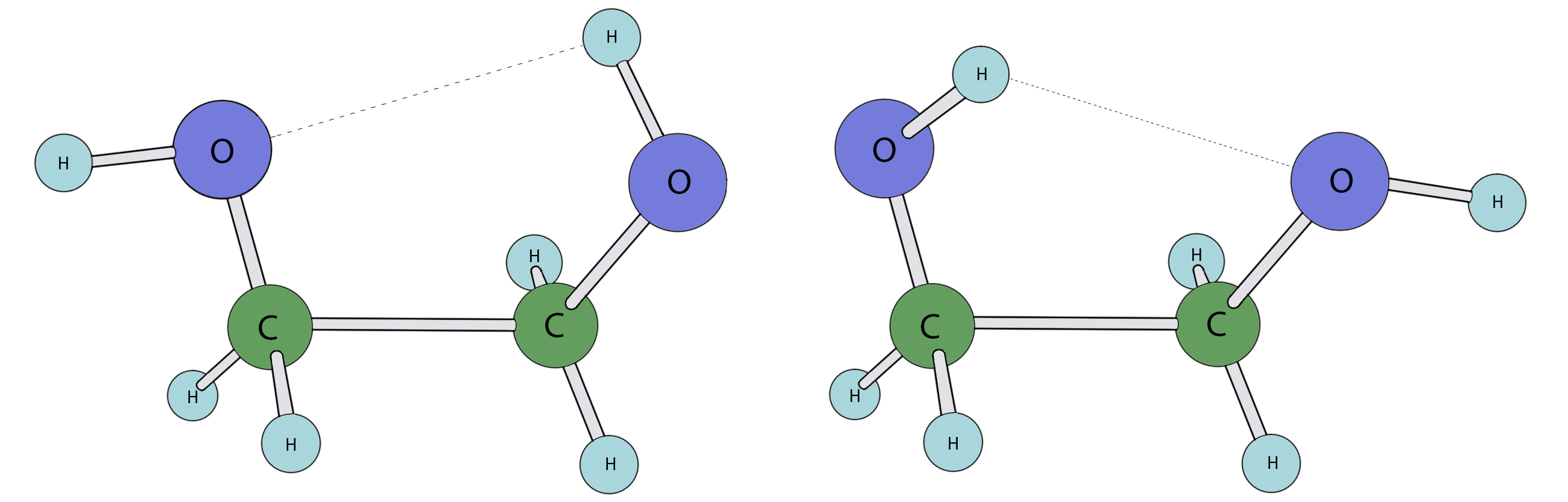
Figure 1: Schematic molecules of ethylene glycol in two degenerate states of the conformation $g^{\prime}Ga$.

Using spectra from extragalactic sources for studying variation of constants was first proposed by Savedoff (1956). Later it was also shown Thompson (1975) that molecular spectra provide a way to determine possible variation of $\mu$. High sensitivity for $\mu$ variation may exist in molecules which have more than one equivalent potential minimum and which can tunnel between these minima van Veldhoven et al. (2004). A well-known example of this kind of molecule is ammonia, $\mathrm{NH_{3}}$, a compound fortunately abundant in interstellar medium (ISM). Mixed tunneling-rotational transitions can be even more sensitive to the change of $\mu$. But highly sensitive transitions of this type can be seen only in asymmetric isotopologues of ammonia, $\mathrm{NH_{2}D}$ and $\mathrm{NHD_{2}}$ Kozlov et al. (2010).

Recently a large number of polyatomic molecules has been observed from the ISM at the redshift $z=0.89$ Muller et al. (2011). That finding stimulated studies of the molecules with mixed tunneling-rotational transitions. Up to now following these molecules have been studied: hydronium ($\mathrm{H_{3}O^{+}}$) Kozlov et al. (2011), hydrogen peroxide ($\mathrm{H_{2}O_{2}}$) Kozlov (2011), methanol ($\mathrm{CH_{3}OH}$) Jansen et al. (2011); Levshakov et al. (2011), methylamine ($\mathrm{CH_{3}NH_{2}}$) Ilyushin et al. (2012), methyl mercaptan ($\mathrm{CH_{3}SH}$) Jansen et al. (2013) and acetaldehyde ($\mathrm{C_{2}H_{4}O}$), acetamide ($\mathrm{CH_{3}CONH_{2}}$), methyl formate ($\mathrm{HCOOCH_{3}}$), acetic acid ($\mathrm{CH_{3}COOH}$) in Jansen et al. (2011). The strongest restriction for $\mu$ variation on a cosmological timescale (4) has been obtained by the observations of methanol spectra at redshift $z=0.89$ Bagdonaite et al. (2013).

We suggest similar consideration of ethylene glycol $\mathrm{C_{2}H_{6}O_{2}}$. It has two equivalent minima in the lowest $g^{\prime}Ga$ conformation, see Fig. 1. Ethylene glycol has been detected in the comet C/1995 O1 (Hale-Bopp) Crovisier et al. (2004) and in ISM to the center of the Milky Way galaxy Hollis et al. (2002); Requena-Torres et al. (2008). Also, recent success in detection of complex organic compounds Muller et al. (2011) at high redshift gives us hope to spot ethylene glycol outside of the Milky Way. Therefore it is important to know which transitions in ethylene glycol are especially sensitive to the change of $\mu$. In this paper we calculate sensitivity coefficients for a large number of transitions, including those which have not been observed yet.

II Method

Let $\omega$ be a present-day experimentally observed transition frequency and $\tilde{\omega}$ a frequency shifted due to possible time (and space) change of $\alpha$ and $\mu$. This shift $\Delta\omega=\tilde{\omega}-\omega$ is linked to $\Delta\alpha$ and $\Delta\mu$ through sensitivity coefficients $Q_{\alpha}$ and $Q_{\mu}$ (we do not consider hyperfine transitions, which may depend on additional parameters, such as nuclear $g$-factors):

$$\frac{\Delta\omega}{\omega}=Q_{\alpha}\frac{\Delta\alpha}{\alpha}+Q_{\mu}\frac{\Delta\mu}{\mu}\,.$$ (5)

For tunneling-rotational spectra of molecules built of light elements ($Z<10$) the sensitivity coefficient $Q_{\alpha}\ll 1$. At the same time typical coefficient $Q_{\mu}\gtrsim 1$. Therefore we neglect $\alpha$-dependence and link $\Delta\omega$ solely with $\Delta\mu$:

$$\frac{\Delta\omega}{\omega}=Q_{\mu}\frac{\Delta\mu}{\mu}\,,$$ (6)

$$\Delta\mu=\tilde{\mu}-\mu\,,\quad|\Delta\mu/\mu|\ll 1\,.$$ (7)

Experimental data for the spectrum of ethylene glycol are taken from Christen et al. (1995).

II.1 Effective Hamiltonian

Ethylene glycol molecule has several conformations, which correspond to the local minima of the potential. The lowest conformation is labeled as $g^{\prime}Ga$ and is twofold degenerate Christen et al. (1995). One can see from Fig. 1 that two equivalent configurations differ mostly by the positions of the two end OH groups. It is this conformation that has been observed in the ISM Hollis et al. (2002); Crovisier et al. (2004); Requena-Torres et al. (2008). Below we discuss effective Hamiltonian for this conformation.

Tunneling motion between two configurations of the $g^{\prime}Ga$ conformation lifts degeneracy and causes 7 GHz energy splitting of the ground state Hollis et al. (2002). For a rotating molecule there is strong Coriolis interaction between large amplitude tunneling mode and overall rotation Christen et al. (1995). Our main goal is to calculate sensitivity coefficients (6) for the tunneling-rotational transitions. To this end we need to define how the parameters of the effective Hamiltonian depend on the electron-to-proton mass ratio $\mu$. This dependence can be reliably established only for the relatively simple Hamiltonians Levshakov et al. (2011); Ilyushin et al. (2012). More sophisticated Hamiltonian can provide better accuracy for the transition frequencies, but do not lead to significant improvement of the accuracy for the sensitivity coefficients.

We found out that reasonable accuracy for the tunneling-rotational spectrum is provided by the 14 parameter Hamiltonian, which in the molecular frame $\xi,\eta,\zeta$ has the form:

$$H_{\mathrm{eff}} =CJ_{\xi}^{2}+BJ_{\eta}^{2}+AJ_{\zeta}^{2}$$ (8a)

$$-\Delta_{J}\bm{J}^{4}-\Delta_{K}J_{\zeta}^{4}-\Delta_{JK}\bm{J}^{2}J_{\zeta}^{2}$$ (8b)

$$+d_{1}\bm{J}^{2}\left(J_{+}^{2}+J_{-}^{2}\right)+d_{2}\left(J_{+}^{4}+J_{-}^{4}\right)$$ (8c)

$$-\frac{\tau}{2}\left(F-W_{C}J_{\xi}^{2}-W_{B}J_{\eta}^{2}-W_{A}J_{\zeta}^{2}\right)$$ (8d)

$$+\left[d_{3}J_{\zeta}+d_{4}\left(J_{+}+J_{-}\right)\right]\delta_{\tau^{\prime},-\tau}\,.$$ (8e)

The first line corresponds to asymmetric top. For ethylene glycol $A\gg B\gtrsim C$, so we can use a basis set $|J,K_{A}\rangle$ for prolate top with $K_{A}\equiv\langle J_{\zeta}\rangle$. Lines (8b,8c) describe diagonal and non-diagonal in $K_{A}$ centrifugal corrections respectively. The line (8d) describes tunneling degree of freedom, where $F$ is tunneling frequency, $\tau=\pm 1$ is tunneling quantum number. Rotational constants weakly depend on the quantum number $\tau$ Christen et al. (1995), so we define $A\equiv(A_{+1}+A_{-1})/2$ and $W_{A}\equiv(A_{+1}-A_{-1})/2$, etc. Parameters $W_{i}$ can be considered as centrifugal corrections to the tunneling frequency $F$ Kozlov et al. (2011). Finally, we introduced two terms (8e), which are non-diagonal in $\tau$ and depend on the rotational quantum numbers. These terms describe Coriolis interaction between rotational degrees of freedom and the tunneling mode. This interaction becomes particularly important when levels with the same quantum number $J$, but different $\tau$ come close to each other. The term $d_{3}$ causes repulsion of such levels with $\Delta K_{A}=0$ and the second one causes repulsion of levels with $\Delta K_{A}=\pm 1$. Addition of these two Coriolis terms to the Hamiltonian improves quality of the fit by more than two orders of magnitude.

Table 1: Modelling of experimental spectrum of ethylene glycol from Ref. Christen et al. (1995) with effective Hamiltonian (8). Frequencies are given in MHz and $\Delta\omega=\omega_{\mathrm{theor}}-\omega_{\mathrm{exper}}$. Quantum numbers $J,K_{A},K_{C}$ correspond to the rigid asymmetric top and $v$ is linked to $\tau$ from (8d): $v=(1-\tau)/2$. Unprimed and primed quantum numbers correspond to upper and lower states respectively. Sensitivity coefficients $\mathrm{Q}_{\mu}$ are calculated as described in Sec. II.2. Estimated theoretical errors are given in parentheses. Two transitions observed to the Galactic centerRequena-Torres et al. (2008) are in boldface.

$J$	$K_{A}$	$K_{C}$	$v\,$	$J^{\prime}$	$K_{A}^{\prime}$	$K_{C}^{\prime}$	$v^{\prime}$	$\omega_{\mathrm{theor}}$	$\omega_{\mathrm{exper}}$	$\Delta\omega$	$Q_{\mu}$
2	2	1	1	2	2	0	0	6889.3	6889.1	$0.2$	$4.0(5)$
5	4	2	1	5	4	1	0	6952.6	6952.0	$0.6$	$4.0(5)$
5	4	1	1	5	4	2	0	6954.6	6953.3	$1.3$	$4.0(5)$
3	3	1	1	3	3	0	0	6956.9	6957.2	$-0.3$	$4.0(5)$
3	3	0	1	3	3	1	0	6962.9	6963.8	$-0.9$	$4.0(5)$
4	4	1	1	4	4	0	0	6964.1	6963.9	$0.2$	$4.0(5)$
4	4	0	1	4	4	1	0	6964.3	6963.9	$0.4$	$4.0(5)$
4	3	1	1	4	3	2	0	6972.4	6972.4	$0.0$	$4.0(5)$
5	3	2	1	5	3	3	0	7024.6	7024.7	$-0.1$	$4.0(5)$
2	2	0	1	2	2	1	0	7026.3	7026.5	$-0.2$	$4.0(5)$
5	1	4	0	5	1	5	1	7600.7	7600.7	$0.0$	$-1.7(4)$
1	1	0	1	1	1	1	0	7925.6	7925.5	$0.1$	$3.6(4)$
4	2	2	1	4	2	3	0	7949.0	7948.9	$0.1$	$3.6(4)$
5	2	3	1	5	1	4	0	9217.5	9217.4	$0.1$	$3.3(4)$
2	1	1	1	2	1	2	0	9852.3	9852.1	$0.2$	$3.1(3)$
2	0	2	1	1	1	1	1	10534.7	10534.5	$0.2$	$0.97(1)$
2	0	2	0	1	1	1	0	10551.8	10551.9	$-0.1$	$1.00(1)$
1	1	0	0	1	0	1	0	10747.6	10747.5	$0.1$	$1.00(1)$
1	1	0	1	1	0	1	1	10754.2	10754.3	$-0.1$	$1.01(1)$
5	1	5	1	4	2	2	1	11488.2	11488.0	$0.2$	$0.99(1)$
5	1	5	1	5	0	5	0	11745.2	11745.0	$0.2$	$2.8(3)$
2	1	1	0	2	0	2	0	11785.9	11785.8	$0.1$	$1.00(1)$
2	1	1	1	2	0	2	1	11810.2	11810.3	$-0.1$	$1.03(1)$
2	1	2	0	1	1	1	1	12492.6	12492.7	$-0.1$	$2.4(3)$
3	1	2	1	3	1	3	0	12689.2	12689.1	$0.1$	$2.4(2)$
$\mathbf{2}$	$\mathbf{0}$	$\mathbf{2}$	$\mathbf{0}$	$\mathbf{1}$	$\mathbf{0}$	$\mathbf{1}$	$\mathbf{1}$	$\mathbf{13380.4}$	$\mathbf{13380.6}$	$\bf-0.\bf 2$	$\bf-0.\bf 6(2)$
3	1	2	0	3	0	3	0	13444.8	13444.8	$0.0$	$1.03(1)$
3	1	2	1	3	0	3	1	13571.4	13571.5	$-0.1$	$1.2(2)$
1	1	0	0	0	0	0	1	13990.8	13990.9	$-0.1$	$-0.5(2)$
2	1	1	0	1	1	0	1	14412.1	14412.2	$-0.1$	$-0.4(2)$
4	1	3	1	3	2	2	1	14678.1	14678.1	$0.0$	$1.00(1)$
4	1	3	0	3	2	2	0	14706.0	14706.2	$-0.2$	$1.02(1)$
4	1	3	1	4	0	4	1	15808.4	15809.0	$-0.6$	$1.1(1)$
4	1	3	0	4	0	4	0	15972.1	15971.9	$0.2$	$1.01(1)$
1	1	1	1	1	0	1	0	16734.2	16734.1	$0.1$	$2.2(2)$
4	1	3	1	4	1	4	0	16786.7	16786.8	$-0.1$	$2.1(2)$
5	2	4	0	5	1	4	1	16897.4	16897.6	$-0.2$	$-0.2(2)$
1	0	1	1	0	0	0	0	17153.8	17153.6	$0.2$	$2.2(2)$
1	1	1	1	0	0	0	1	19977.4	19977.5	$-0.1$	$1.00(1)$
1	1	1	0	0	0	0	0	19982.4	19982.3	$0.1$	$1.00(1)$
$\mathbf{3}$	$\mathbf{0}$	$\mathbf{3}$	$\mathbf{0}$	$\mathbf{2}$	$\mathbf{0}$	$\mathbf{2}$	$\mathbf{1}$	$\mathbf{23392.9}$	$\mathbf{23393.0}$	$\bf-0.\bf 1$	$\bf 0.\bf 1(1)$
3	1	2	0	2	1	1	1	25027.5	25027.6	$-0.1$	$0.2(1)$
3	2	1	1	3	1	2	1	28259.1	28259.3	$-0.2$	$1.00(1)$
3	2	1	0	3	1	2	0	28292.2	28291.9	$0.3$	$0.98(1)$
4	0	4	0	3	0	3	1	33272.8	33272.9	$-0.1$	$0.5(1)$
3	2	2	0	3	1	3	0	33656.7	33656.4	$0.3$	$0.9(1)$
4	2	3	0	3	2	2	1	33806.6	33806.3	$0.3$	$0.4(1)$
4	3	2	0	3	3	1	1	33977.3	33976.8	$0.5$	$0.4(1)$
4	3	1	0	3	3	0	1	33995.2	33994.6	$0.6$	$0.4(1)$
4	1	3	0	3	1	2	1	35673.5	35673.4	$0.1$	$0.4(1)$
4	2	3	0	4	1	4	0	35915.2	35915.1	$0.1$	$0.9(1)$
3	1	3	1	2	1	2	0	36061.4	36061.5	$-0.1$	$1.6(1)$
3	0	3	1	2	0	2	0	37188.1	37187.7	$0.4$	$1.5(1)$
3	2	2	1	2	2	1	0	37557.0	37557.2	$-0.2$	$1.6(1)$
3	1	3	1	2	0	2	1	38019.3	38019.7	$-0.4$	$1.00(1)$
3	1	3	0	2	0	2	0	38070.3	38070.2	$0.1$	$1.1(1)$
5	2	4	1	5	1	5	1	38351.8	38351.8	$0.0$	$1.00(1)$
3	1	2	1	2	1	1	0	38973.6	38973.4	$0.2$	$1.5(1)$
5	0	5	0	4	0	4	1	42628.9	42629.1	$-0.2$	$0.6(1)$
5	2	4	0	4	2	3	1	43919.9	43919.7	$0.2$	$0.5(1)$
5	4	2	0	4	4	1	1	44199.5	44199.7	$-0.2$	$0.5(1)$
5	4	1	0	4	4	0	1	44200.4	44200.6	$-0.2$	$0.5(1)$
5	3	3	0	4	3	2	1	44264.4	44263.9	$0.5$	$0.5(1)$
5	3	2	0	4	3	1	1	44326.3	44326.0	$0.3$	$0.5(1)$
5	2	3	0	4	2	2	1	45180.0	45179.7	$0.3$	$0.5(1)$
4	1	4	1	3	1	3	0	45547.5	45547.6	$-0.1$	$1.4(1)$
5	1	4	0	4	1	3	1	46166.4	46166.5	$-0.1$	$0.6(1)$
4	0	4	1	3	0	3	0	47217.7	47217.4	$0.3$	$1.4(1)$
4	2	3	1	3	2	2	0	47696.1	47696.4	$-0.3$	$1.4(1)$
4	3	2	1	3	3	1	0	47888.3	47888.7	$-0.4$	$1.4(1)$
4	3	1	1	3	3	0	0	47906.6	47906.9	$-0.3$	$1.4(1)$
4	2	2	1	3	2	1	0	48366.6	48366.8	$-0.2$	$1.4(1)$
4	1	3	0	3	0	3	1	49244.9	49245.2	$-0.3$	$0.6(1)$
4	1	3	1	3	1	2	0	49581.3	49581.1	$0.2$	$1.4(1)$
5	3	2	1	5	2	3	1	49690.5	49690.6	$-0.1$	$1.00(1)$
3	1	2	1	2	0	2	0	50759.5	50759.3	$0.2$	$1.4(1)$
5	1	5	1	4	1	4	0	55352.4	55352.7	$-0.3$	$1.3(1)$
5	2	4	1	4	2	3	0	57789.0	57789.2	$-0.2$	$1.4(1)$
5	3	2	1	4	3	1	0	58219.2	58219.4	$-0.2$	$1.4(1)$
5	2	3	1	4	2	2	0	59076.2	59076.3	$-0.1$	$1.4(1)$

II.2 Determining $\mu$-dependence of the effective Hamiltonian

Below we find parameters of the effective Hamiltonian (8) from the fit to the experimental spectrum Christen et al. (1995). However, we assume that, in principle, these parameters can be found from the ab initio calculations. Repeating such calculations with different values of $\mu$ we can find $\mu$-dependence of our parameters. On the other hand, at least for the largest parameters of our Hamiltonian we can find approximate $\mu$-dependence without extensive calculations. For example, rotational constants scale as $1/(MR^{2})$, where $M$ is nuclear mass and $R$ is equilibrium internuclear distance. This means that in atomic units, which are traditionally used to define sensitivity coefficients, the rotational constants $A,\,B,\,C$ scale as $\mu^{1}$. Similar arguments show that centrifugal corrections $\Delta_{J},\,\Delta_{K},\,\Delta_{JK}$ and $d_{1},\,d_{2}$ scale as $\mu^{2}$. The accuracy of these scalings is on the order of 1%, or so Levshakov et al. (2011); Ilyushin et al. (2012). Without calculating these scalings more accurately we can not improve the accuracy for the sensitivity coefficients $Q_{\mu}$ by adding higher centrifugal corrections to our Hamiltonian.

In order to find $\mu$-dependence of the constant $F$ we can either do some model calculations for the tunneling mode Flambaum and Kozlov (2007); Kozlov et al. (2011), or use experimental data for the deuterated species van Veldhoven et al. (2004). We use the latter approach here. Using semiclassical arguments we can expect following scaling of the parameter $F$:

$$F=a\mu^{1/2}\exp\left(-b/\mu^{1/2}\right)\,,$$ (9)

$$Q_{\mu}(F)=\frac{1}{2}\left(1+b/\mu^{1/2}\right)\,.$$ (10)

We can find parameters $a$ and $b$ from experimental values of $F$ for two isotopologues of ethylene glycol: $F=6958$ MHz for HOCH₂CH₂OH and $F=293$ MHz for DOCH₂CH₂OD Christen et al. (1995). We consider deuterated molecule as one with a proton of a double mass.

According to Fig. 1 two degenerate configurations differ mostly by the positions of the OH (or OD) groups. We do not know the exact tunneling path and the respective effective tunneling mass. In the two limiting models the tunneling motion can be approximated as a rotation of the rigid OH groups, or simply as the motion of two hydrogen atoms. In the first case the tunneling masses for two isotopologues are $M_{1}=M_{\rm H}M_{\rm O}/(M_{\rm H}+M_{\rm O})$ and $M_{2}=M_{\rm D}M_{\rm O}/(M_{\rm D}+M_{\rm O})$. In the second case $M_{1}=M_{\rm H}$ and $M_{2}=M_{\rm D}$. For the first case we get $Q_{\mu}(F)=4.31$ and for the second case $Q_{\mu}(F)=3.91$. Actual tunneling mass should lie between these two limiting cases, so the conservative estimate is:

$$Q_{\mu}(F)=4.1\pm 0.2\,.$$ (11)

Finally we need to determine $\mu$-dependence for centrifugal corrections to the tunneling frequency $W_{i}$ and Coriolis parameters $d_{3}$ and $d_{4}$. At present there is no accurate theory for these terms, but it is usually assumed Jansen et al. (2011); Ilyushin et al. (2012) that their scaling with $\mu$ is given by a product of lower-order Hamiltonian terms, in this case the tunneling and rotational constants. The sensitivity coefficients for the higher-order terms are thus given by

$$Q_{\mu}(W_{i})=Q_{\mu}(d_{3})=Q_{\mu}(d_{4})=Q_{\mu}(F)+1\,.$$ (12)

Knowing the scalings of the parameters of the effective Hamiltonian we can find $\mu$ dependence of the transition frequencies by diagonalizing $H_{\mathrm{eff}}$ for several sets of parameters, which corresponds to different values of $\mu$.

Table 2: Optimized parameters of the effective Hamiltonian (8) in MHz.

$A$	$15363.284$
$B$	$5587.121$
$C$	$4613.531$
$\Delta_{J}$	$0.0074$
$\Delta_{K}$	$0.0774$
$\Delta_{JK}\quad$	$-0.0329$
$d_{1}$	$0.0025$
$d_{2}$	$0.00003$
$F$	$6958.1$
$W_{C}$	$13.088$
$W_{B}$	$-0.425$
$W_{A}$	$2.771$
$d_{3}$	$217.09$
$d_{4}$	$50.83$

III Numerical results and discussion

The lowest part of the tunneling-rotational spectrum of ethylene glycol is shown in Fig. 2. Effective Hamiltonian discussed above is used to model the spectrum and to calculate corresponding sensitivities $Q_{\mu}$. We fit 14 parameters from Eq. (8) to the experimental transition frequencies measured by Christen et al. (1995). Typical temperature of the ISM is $T\lesssim 10$K, so the levels with $J>5$ are weakly populated. Transitions for higher $J$’s observed in Hollis et al. (2002) correspond to the much warmer gas and are very broad (linewidths $>$ 20 km/s). Because of that we use Hamiltonian, which includes only lowest centrifugal corrections and restrict our consideration to the levels with $J\leq 5$. Results of this fit are presented in Table LABEL:tab1. Achieved agreement is quite satisfactory taking into account relative simplicity of the model we use. The maximum deviation $\Delta\omega$ from the measured frequency is 1.3 MHz, while the rms deviation is about 0.3 MHz.

The optimized parameters of the model are listed in Table 2. One can see that centrifugal and Coriolis corrections to the tunneling are rather large. The largest term $d_{3}$ causes up to a hundred MHz shifts of several transition lines. Being nondiagonal in the quantum number $\tau$ the terms $d_{3}$ and $d_{4}$ become important only for the close levels with the opposite values of $\tau$ and the same $J$. There are only several such levels with $J\leq 5$. Other terms of the Hamiltonian contribute more uniformly to the tunneling-rotational spectrum of the molecule.

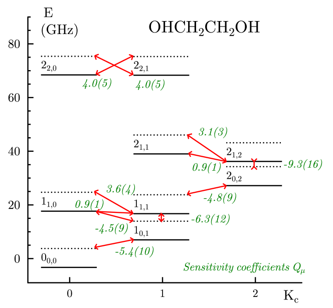
Figure 2: The lowest part of the tunneling-rotational spectrum of ethylene glycol. Quantum numbers of energy levels are given as $J_{K_{a},K_{c}}$. Solid lines correspond to $v=0$, dotted ones to $v=1$. Sensitivity coefficients $Q_{\mu}$ are in italic. Note that predominantly rotational transitions ($\Delta v=0$) have $Q_{\mu}\approx 1$.

Table 3: Predicted low-frequency tunneling-rotational transitions (in the range from 800 MHz to 6.8 GHz) and their sensitivity coefficients $Q_{\mu}$. Frequencies are in MHz and wavelengths are in cm. Other notations are the same as in Table LABEL:tab1.

$J$	$K_{A}$	$K_{C}$	$v\,$	$J^{\prime}$	$K_{A}^{\prime}$	$K_{C}^{\prime}$	$v^{\prime}$	$\omega$	$\lambda$	$Q_{\mu}$
3	1	3	0	3	0	3	1	882.2	34.0	$-16.5(58)$
1	1	0	0	1	1	1	0	966.4	31.0	$0.9(1)$
4	0	4	1	4	1	4	0	978.3	30.6	$17.8(38)$
4	2	2	0	4	2	3	0	1000.9	30.0	$0.95(1)$
3	1	3	1	3	1	2	0	1181.6	25.4	$17.9(26)$
2	1	2	0	2	0	2	1	1957.9	15.3	$-9.3(16)$
3	3	1	0	4	2	2	1	2641.3	11.4	$-6.9(12)$
3	1	2	0	2	2	1	0	2653.8	11.3	$1.2(2)$
3	1	2	1	2	2	1	1	2682.2	11.2	$0.98(2)$
4	1	3	0	4	1	4	1	2815.2	10.7	$-6.2(11)$
1	1	1	0	1	0	1	1	2828.6	10.6	$-6.3(12)$
2	1	1	0	2	1	2	0	2892.1	10.4	$0.9(1)$
1	0	1	0	0	0	0	1	3243.2	9.2	$-5.4(10)$
2	0	2	0	1	1	1	1	3598.8	8.3	$-4.8(9)$
1	1	0	0	1	0	1	1	3795.0	7.9	$-4.5(9)$
2	1	2	1	2	1	1	0	4043.9	7.4	$6.2(8)$
2	2	1	1	3	1	2	0	4303.7	7.0	$5.8(7)$
2	1	1	0	2	0	2	1	4850.0	6.2	$-3.2(7)$
3	1	2	0	3	1	3	0	5703.3	5.3	$0.6(5)$
4	2	3	1	4	2	2	0	5938.8	5.0	$4.5(5)$
1	1	1	1	1	1	0	0	5986.6	5.0	$4.5(5)$
4	1	4	0	4	0	4	0	6107.3	4.9	$1.4(3)$
3	1	2	0	3	0	3	1	6585.5	4.6	$-1.7(4)$
3	2	2	1	3	2	1	0	6611.0	4.5	$4.2(5)$

In the experiment Christen et al. (1995) only transitions above 6.8 GHz were detected. At the same time, we are primarily interested in low frequency mixed tunneling-rotational transitions with $\omega\gtrsim 1$ GHz, where high sensitivities are possible. Transitions with even lower frequencies are hardly detectable by modern Earth based radio telescopes. To the best of our knowledge such transitions for ethylene glycol were never seen. Thus, we used our effective Hamiltonian with optimal parameters from Table 2 to search for such low frequency transitions. We again restricted ourselves to $J\leq 5$ where our model has been tested against the experiment and proved to be quite reliable. Within these limits we found 24 low frequency transitions listed in Table 3. Some of them are shown in Fig. 2. We estimate the accuracy of the predicted frequencies to be about 0.5 MHz.

We used the same optimal effective Hamiltonian to calculated sensitivities $Q_{\mu}$ for all transitions from Tables LABEL:tab1 and 3 as was described in Sec. II.2. In order to estimate the uncertainty for the obtained $Q$ factors we made several additional calculations. The main error comes from the uncertainty (11), so we first calculated sensitivities for maximum and minimum values of $Q_{\mu}(F)$.

As we pointed out above, the theoretical grounds for Eq. (12) are not very solid. Therefore we repeated calculations of the $Q$ factors with smaller number of fitting parameters. In particular, we successively turned each of the parameters $d_{i}$ and $W_{i}$ to zero and made fits for remaining 13 parameter sets. After that we calculated sensitivity coefficients $Q_{\mu}$ for such restricted parameter sets. Note that according to Eq. (6) the value of $Q_{\mu}$ is inversely proportional to the transition frequency $\omega$. For the low frequency transitions predicted frequency may be quite sensitive to the values of the parameters and can be significantly different for the best fit and for the restricted fits. This part of the error is trivial and can be easily eliminated for example by using the experimental frequencies instead of the calculated ones. Because of that we excluded this error by using frequencies from the best fit in the denominator, while the frequency shift $\Delta\omega$ in the numerator was recalculated for each restricted set of parameters.

After all these calculations being done we estimate the error $\Delta Q_{\mu}$ for each transition by taking maximum deviation from the main calculation with optimal parameters. In most cases maximum error comes from the uncertainty in the value of $Q_{\mu}(F)$. However, for some important transitions with high sensitivities the largest deviation corresponds to the fit with $d_{4}$ set to zero. The optimal value of this parameter is rather large and setting it to zero significantly influences both the frequencies and their $\mu$ dependence. The error associated with the parameter $d_{4}$ is particularly large for some of the most interesting low-frequency transitions. On the contrary, transitions with sensitivities close to unity are not sensitive to any changes of the parameters discussed above. Here the main error comes from the uncertainty to which we know $\mu$ dependence of the rotational constants. In Refs. Levshakov et al. (2011); Ilyushin et al. (2012) this error was estimated to be about 1%. This is the minimal error of our calculation for the predominantly rotational transitions with $Q_{\mu}\approx 1$.

Conclusion

During last few years the molecules with mixed tunneling-rotational spectra proved to be very useful for constraining possible $\mu$ variation on the large space-time scale. Current most stringent limit on such variation has been obtained with methanol Bagdonaite et al. (2013). There is large variability in the abundances of different species in the ISM and in observed intensities of different molecular lines. Because of that it is useful to study all potentially interesting molecules and transitions. In this paper we considered one of the last unstudied relatively simple molecules with the tunneling mode.

We found several low frequency transitions in the range between 0.8 and 7 GHz with high sensitivity to $\mu$ variation of both signs. Note that it is the difference in sensitivities that is important for the observation of $\mu$-variation. The maximum difference in sensitivities for these transitions is close to 34. This is comparable to the differences earlier found for methanol Jansen et al. (2011); Levshakov et al. (2011). For a higher frequencies there are several transitions around 7.0 GHz with sensitivities $Q_{\mu}\approx 4.0$ and one transition at 7.6 GHz with sensitivity $Q_{\mu}\approx-1.7$. Small frequency differences may help to observe these lines simultaneously, minimizing possible systematic errors.

Ethylene glycol has been detected in the ISM Hollis et al. (2002); Requena-Torres et al. (2008), which makes it one of the perspective candidates for the search for $\mu$ variation. Observed lines from the cold molecular clouds in the Milky Way can be very narrow allowing for high precision spectroscopy. This can be used Molaro et al. (2009); Levshakov et al. (2011); Ellingsen et al. (2011) to study the possible dependence of the electron-to-proton mass ratio on the local matter density, which is predicted by models with chameleon scalar fields Khoury and Weltman (2004); Olive and Pospelov (2008). At the same time high redshift observations of the tunneling-rotational lines can be used to study $\mu$ variation on the cosmological timescale Ellingsen et al. (2012); Bagdonaite et al. (2013).

We thank Sergei Levshakov for helpful discussions. This work is partly supported by the Russian Foundation for Basic Research, Grant No. 14-02-00241.

References

- Dirac (1937) P. A. M. Dirac, Nature 139, 323 (1937).
- Damour (2012) T. Damour, Classical and Quantum Gravity 29, 184001 (2012), arxiv:1202.6311.
- Khoury and Weltman (2004) J. Khoury and A. Weltman, Phys. Rev. Lett. 93, 171104 (2004), arXiv:astro-ph/0309300 .
- Olive and Pospelov (2008) K. A. Olive and M. Pospelov, Phys. Rev. D 77, 043524 (2008), arXiv:0709.3825 .
- Barrow and Lip (2012) J. D. Barrow and S. Z. W. Lip, Phys. Rev. D 85, 023514 (2012), arXiv:1110.3120 .
- Uzan (2011) J.-P. Uzan, Living Reviews in Relativity 14, 2 (2011).
- Rosenband et al. (2008) T. Rosenband, D. B. Hume, P. O. Schmidt, C. W. Chou, A. Brusch, L. Lorini, W. H. Oskay, R. E. Drullinger, T. M. Fortier, J. E. Stalnaker, S. A. Diddams, W. C. Swann, N. R. Newbury, W. M. Itano, D. J. Wineland, and J. C. Bergquist, Science 319, 1808 (2008).
- Cingöz et al. (2007) A. Cingöz, A. Lapierre, A.-T. Nguyen, N. Leefer, D. Budker, S. K. Lamoreaux, and J. R. Torgerson, Phys. Rev. Lett. 98, 040801 (2007), arXiv:physics/0609014 .
- Shelkovnikov et al. (2008) A. Shelkovnikov, R. J. Butcher, C. Chardonnet, and A. Amy-Klein, Phys. Rev. Lett. 100, 150801 (2008), arXiv:0803.1829 .
- Ferreira et al. (2012) M. C. Ferreira, M. D. Julião, C. J. A. P. Martins, and A. M. R. V. L. Monteiro, Phys. Rev. D 86, 125025 (2012), arXiv:1212.4164 .
- Blatt et al. (2008) S. Blatt, A. D. Ludlow, G. K. Campbell, J. W. Thomsen, T. Zelevinsky, M. M. Boyd, J. Ye, X. Baillard, M. Fouché, R. Le Targat, A. Brusch, P. Lemonde, M. Takamoto, F.-L. Hong, H. Katori, and V. V. Flambaum, Physical Review Letters 100, 140801 (2008), arXiv:0801.1874 .
- Petrov et al. (2006) Y. V. Petrov, A. I. Nazarov, M. S. Onegin, V. Y. Petrov, and E. G. Sakhnovsky, Phys. Rev. C 74, 064610 (2006), arXiv:hep-ph/0506186 .
- Levshakov et al. (2012) S. A. Levshakov, F. Combes, F. Boone, I. I. Agafonova, D. Reimers, and M. G. Kozlov, Astron. Astrophys. 540, L9 (2012).
- Bagdonaite et al. (2013) J. Bagdonaite, P. Jansen, C. Henkel, H. L. Bethlem, K. M. Menten, and W. Ubachs, Science 339, 46 (2013).
- Webb et al. (2011) J. K. Webb, J. A. King, M. T. Murphy, V. V. Flambaum, R. F. Carswell, and M. B. Bainbridge, Phys. Rev. Lett. 107, 191101 (2011), arXiv:1008.3907.
- Savedoff (1956) M. P. Savedoff, Nature 178, 688 (1956).
- Thompson (1975) R. I. Thompson, Astrophys. Lett. 16, 3 (1975).
- van Veldhoven et al. (2004) J. van Veldhoven, J. Küpper, H. L. Bethlem, B. Sartakov, A. J. A. van Roij, and G. Meijer, Eur. Phys. J. D 31, 337 (2004).
- Kozlov et al. (2010) M. G. Kozlov, A. V. Lapinov, and S. A. Levshakov, J. Phys. B 43, 074003 (2010), arXiv:0908.2983 .
- Muller et al. (2011) S. Muller, A. Beelen, M. Guélin, S. Aalto, J. H. Black, F. Combes, S. Curran, P. Theule, and S. Longmore, Astron. Astrophys. 535, A103 (2011), arXiv:1104.3361.
- Kozlov et al. (2011) M. G. Kozlov, S. G. Porsev, and D. Reimers, Phys. Rev. A 83, 052123 (2011), arXiv:1103.4739 .
- Kozlov (2011) M. G. Kozlov, Phys. Rev. A 84, 042120 (2011), arXiv:1108.4520 .
- Jansen et al. (2011) P. Jansen, L.-H. Xu, I. Kleiner, W. Ubachs, and H. L. Bethlem, Phys. Rev. Lett. 106, 100801 (2011).
- Levshakov et al. (2011) S. A. Levshakov, M. G. Kozlov, and D. Reimers, Astrophys. J. 738, 26 (2011), arXiv:1106.1569 .
- Ilyushin et al. (2012) V. V. Ilyushin, P. Jansen, M. G. Kozlov, S. A. Levshakov, I. Kleiner, W. Ubachs, and H. L. Bethlem, Phys. Rev. A 85, 032505 (2012).
- Jansen et al. (2013) P. Jansen, L.-H. Xu, I. Kleiner, H. L. Bethlem, and W. Ubachs, Phys. Rev. A 87, 052509 (2013), arxiv:1304.5249.
- Jansen et al. (2011) P. Jansen, I. Kleiner, L.-H. Xu, W. Ubachs, and H. L. Bethlem, Phys. Rev. A 84, 062505 (2011), eprint arXiv:1109.5076.
- Crovisier et al. (2004) J. Crovisier, D. Bockelée-Morvan, N. Biver, P. Colom, D. Despois, and D. C. Lis, Astron. Astrophys. 418, L35 (2004).
- Hollis et al. (2002) J. M. Hollis, F. J. Lovas, P. R. Jewell, and L. H. Coudert, Astrophys. J. 571, L59 (2002).
- Requena-Torres et al. (2008) M. A. Requena-Torres, J. Martín-Pintado, S. Martín, and M. R. Morris, Astrophys. J. 672, 352 (2008).
- Christen et al. (1995) D. Christen, L. H. Coudert, R. D. Suenram, and F. J. Lovas, Journal of Molecular Spectroscopy 172, 57 (1995).
- Flambaum and Kozlov (2007) V. V. Flambaum and M. G. Kozlov, Phys. Rev. Lett. 98, 240801 (2007), arXiv:0704.2301 .
- Molaro et al. (2009) P. Molaro, S. A. Levshakov, and M. G. Kozlov, Nuclear Physics B Proceedings Supplements 194, 287 (2009), arXiv:0907.1192 .
- Ellingsen et al. (2011) S. Ellingsen, M. Voronkov, and S. Breen, Phys. Rev. Lett. 107, 270801 (2011), arXiv:1111.4708 .
- Ellingsen et al. (2012) S. P. Ellingsen, M. A. Voronkov, S. L. Breen, and J. E. J. Lovell, Astrophys. J. 747, L7 (2012), arXiv:1201.5644.