A 3D BABCOCK-LEIGHTON SOLAR DYNAMO MODEL

Abstract

We present a 3D kinematic solar dynamo model in which poloidal field is generated by the emergence and dispersal of tilted sunspot pairs (more generally Bipolar Magnetic Regions, or BMRs). The axisymmetric component of this model functions similarly to previous 2D Babcock-Leighton (BL) dynamo models that employ a double-ring prescription for poloidal field generation but we generalize this prescription into a 3D flux emergence algorithm that places BMRs on the surface in response to the dynamo-generated toroidal field. In this way, the model can be regarded as a unification of BL dynamo models (2D in radius/latitude) and surface flux transport models (2D in latitude/longitude) into a more self-consistent framework that captures the full 3D structure of the evolving magnetic field. The model reproduces some basic features of the solar cycle including an 11-yr periodicity, equatorward migration of toroidal flux in the deep convection zone, and poleward propagation of poloidal flux at the surface. The poleward-propagating surface flux originates as trailing flux in BMRs, migrates poleward in multiple non-axisymmetric streams (made axisymmetric by differential rotation and turbulent diffusion), and eventually reverses the polar field, thus sustaining the dynamo. In this letter we briefly describe the model, initial results, and future plans.

1. INTRODUCTION

Babcock (1961) was the first to describe how the emergence of toroidal magnetic flux through the solar surface and the subsequent evolution of that flux can produce a large-scale poloidal magnetic field. Furthermore, he argued that this process, together with the generation of toroidal field by differential rotation (the $\Omega$-effect) gives rise to the 11-yr solar activity cycle. Later work beginning with Leighton (1964, 1969) fleshed out Babcock’s vision and transformed it into viable numerical dynamo models of the solar cycle.

Though many alternative solar dynamo models have been proposed, the Babcock-Leighton (BL) paradigm has remained compelling because it is firmly grounded in solar observations and provides a robust mechanism for producing cyclic dynamo activity (see reviews by Dikpati & Gilman, 2009; Charbonneau, 2010). One of the major milestones in model development occurred in the 1990s when meridional circulation was included and was shown to play a crucial role in regulating the cycle period and other cycle features such as the poleward drift of photospheric flux and the phasing of polar field reversals (Wang & Sheeley, 1991; Choudhuri et al., 1995; Dikpati & Charbonneau, 1999). In recognition of the importance of flux transport by meridional circulation, these new BL models were christened Flux-Transport (FT) dynamo models and remain popular today.

Though they ostensibly rely on flux emergence and evolution in order to operate, most early BL/FT models did not explicitly include sunspots. instead, the generation of poloidal field through the BL mechanism was represented as an idealized axisymmetric source term in the poloidal component of the magnetohydrodynamic (MHD) induction equation. This BL source term is often nonlocal in the sense that it is confined to the surface layers, but its amplitude is proportional to the strength of the toroidal field near the bottom of the convection zone (CZ). The 2D (axisymmetric) MHD induction equation is then solved to follow the evolution of kinematic, axisymmetric (longitudinally-averaged) mean fields.

Another milestone in model development was to replace the non-local $\alpha$-effect with a more phenomenological representation of tilted sunspot pairs. This was originally done in an axisymmetric context through Durney’s (1997) double-ring algorithm which represents a tilted sunspot pair as two overlapping toroidal rings with opposite polarity. This algorithm was later extended and implemented into 2D BL/FT dynamo models by Nandy & Choudhuri (2001), Munoz-Jaramillo et al. (2010) and Guerrero et al. (2012).

A more sophisticated 3D flux emergence algorithm was recently presented by Yeates & Munoz-Jaramillo (2013; hereafter YM13). To our knowledge, this is the first use of a fully 3D Babcock-Leighton source term. In their model, YM13 model flux emergence through an imposed helical flow that lifts and twists the dynamo-generated toroidal field such that it emerges through the surface and then evolves according to the action of turbulent diffusion and mean fields.

Here we explore an alternative approach to a 3D kinematic BL/FT model. Rather than imposing a flow to advect the magnetic field upward as in YM13, we place a spot pair (or, more generally a Bipolar Magnetic Region, or BMR; cf. YM13) confined to the surface layers above the position where the subsurface toroidal flux peaks. Since the mean-field component of the 3D induction equation is equivalent to a corresponding double-ring algorithm, this approach makes closer contact with previous 2D (latitude-radius) BL/FT dynamo models. Furthermore, Since the emergent field is confined to the surface layers, it makes closer contact with a seperate class of models known as surface flux transport (SFT) models that follow the 2D (latitude/longitude) evolution of emergent flux in the solar photosphere subject to mean flows and turbulent diffusion (Leighton, 1964; Wang & Sheeley, 1991; Schrijver, 2001; Baumann et al., 2006).

In summary, our model is a unification of BL/FT dynamo models and SFT models. Though it is not the first such unification (see Munoz-Jaramillo et al. 2010, YM13), it is a promising approach that we intend to pursue in the future to study the 3D evolution of the cyclic solar magnetic field and its coupling to the corona and heliosphere. We describe the basic model components in §2 and the flux emergence algorithm in §3. We then present illustrative results, conclusions, and future plans in §4.

2. DEVELOPMENT OF 3D BABCOCK-LEIGHTON DYNAMO MODEL

Building on the success of previous 2D BL/FT dynamo models, we construct a 3D solar dynamo model by solving the MHD induction equation in the kinematic limit

$$\frac{\partial{\bf B}}{\partial t}=\mbox{\boldmath$\nabla\times$}\left({\bf v}\mbox{\boldmath$\times$}{\bf B}-\eta_{t}\mbox{\boldmath$\nabla\times$}{\bf B}\right)$$ (1)

where $\eta_{t}(r)$ is a turbulent diffusion, and solar velocity fields are specified based on photospheric observations and helioseismic inversions. We use spherical polar coordinates ($r$,$\theta$,$\phi$) throughout. Unlike many mean-field dynamo models, we do not include an explicit $\alpha$-effect. Instead, the dynamo is sustained by the appearance and evolution of sunspot pairs (BMRs) which are placed on the surface in response to the dynamo-generated field by the “Spotmaker” algorithm described in §3.

In this introductory paper, the velocity field ${\bf v}$ is axisymmetric, consisting only of differential rotation and meridional circulation. In this case the evolution of the mean field $\left<{\bf B}\right>$ (brackets denote an average over longitude, $\phi$) is independent of modes with higher azimuthal wavenumbers ($m>0$). This can be verified by averaging eq. (1) over longitude. Thus, from the perspective of the mean fields, the Spotmaker algorithm is equivalent to the the double-ring approach used in previous 2D BL/FT dynamo models (Durney, 1997; Nandy & Choudhuri, 2001; Munoz-Jaramillo et al., 2010; Guerrero et al., 2012), though details such as the spatial profiles and temporal cadence of the spot appearances are different. We view this as beneficial at this stage in the model development because it allows us to make direct contact with existing 2D BL/FT models. Future modeling will incorporate non-axisymmetric flow fields and nonlinear feedbacks (see §4) which will break this degeneracy with 2D models but for now it provides an auspicious framework to build upon previous work.

The framework of the model is built upon the ASH (Anelastic Spherical Harmonic) code described by Clune et al. (1999) and Brun et al. (2004). ASH is a workhorse code that has been applied extensively to simulate solar and stellar convection (see Miesch, 2005; Brun, 2010) but here we use it in a kinematic mode to solve only the induction equation. The numerical method is pseudospectral, with a triangularly-truncated spherical harmonic decomposition in the horizontal dimensions and mixed semi-implicit/explicit timestepping. This version of the ASH code uses a fourth-order finite difference formulation in the radial dimension.

The differential rotation and meridional circulation that comprise ${\bf v}$ are expressed in terms of an angular velocity profile $\Omega(\theta,r)$ and a mass flux stream flunction $\Psi(\theta,r)$ with the same formulations and parameter values used in the 2D models of Dikpati (2011). For the turbulent diffusion $\eta_{t}$ we use the two-step profile described by Dikpati & Gilman (2007).

3. FLUX EMERGENCE ALGORITHM: SPOTMAKER

Our objective is to construct a solar dynamo model that captures both the solar activity cycle and the observed evolution of large-scale magnetic flux solar surface. However, capturing the full complexity of active region formation and dispersal through is currently beyond the capability of a single numerical dynamo model. Here we use an idealized flux emergence algorithm to place spots on the solar surface in response to the dynamo-generated toroidal field near the base of the CZ. As mentioned in §1 this algorithm can be regarded as a 3D generalization of the axisymmetric double-ring algorithm of Durney (1997) and Munoz-Jaramillo et al. (2010).

The first step in the algorithm is to define a spot-producing toroidal flux near the base of the CZ as follows

$$\hat{B}_{\phi}(\theta,\phi,t)=\int_{r_{a}}^{r_{b}}h(r)B_{\phi}(r,\theta,\phi,t)dr$$ (2)

where $h(r)=h_{0}\left(r-r_{a}\right)\left(r_{b}-r\right)$ and $h_{0}$ is defined such that $\int_{r_{a}}^{r_{b}}h(r)dr=1$. This is similar to analogous expressions used by Rempel (2006), but unlike previous models, the flux $\hat{B}_{\phi}(\theta,\phi,t)$ is not necessarily axisymmetric; longitudinal structure is permitted in the toroidal bands that give rise to active regions.

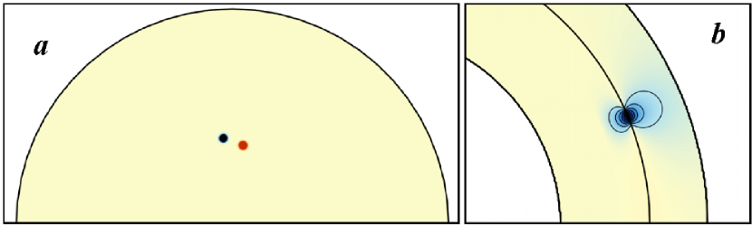
Figure 1.— Structure of a spot pair generated by the flux emergence algorithm, Spotmaker. ($a$) orthographic projection of radial field at the solar surface illustrating a mid-latitude spot with a Joy’s law tilt. Blue and red denote inward and outward field respectively. ($b$) Mean (axisymmetric) component of the poloidal field associated with the tilted spot pair. Colors and contours correspond to the magnetic potential $\Gamma$, with blue denoting a counter-clockwise field orientation. Here the penetration radius $r_{p}=0.95R$.

The next step is to suppress sunspot formation at high latitudes. This is empirically motivated but may have a dynamical explanation in terms of the disruption of high-latitude toroidal flux systems by the magneto-rotational instability (Parfrey & Menou, 2007). We accomplish this by applying a mask to $\hat{B}_{\phi}(\theta,\phi,t)$ such that

$$B^{*}(\theta,\phi,t)=\frac{2g_{0}|\sin\theta\cos\theta|}{1+\exp[-\gamma_{s}\theta^{\prime}]}~{}~{}\hat{B}(\theta,\phi,t)~{}~{}~{},$$ (3)

where $\theta^{\prime}=\theta-\pi/4$ in the northern hemisphere (NH) and $3\pi/4-\theta$ in the southern hemisphere (SH). Here we use $\gamma_{s}=30$ and choose the normalization $g_{0}$ such that the maximum value of the masking function is unity (see Dikpati et al., 2004).

The placement of a spot pair in latitude and longitude is given by the location where the amplitude of $B^{*}(\theta,\phi,t)$ is maximum. If this occurs over a broad range of longitude (for example, from axisymmetric initial conditions), then a longitude is chosen at random from those locations where $B^{*}(\theta,\phi,t)$ is within 0.1% of its peak value.

A spot is placed if the maximum amplitude of $B^{*}$ exceeds a threshold value $B_{t}$. However, in order to avoid introducing overlapping spots at every time step, a time delay is also required. This can be loosely regarded as a dynamical adjustment time between flux emergence events. Here we use a cumulative lognormal distribution function defined as

$${\cal C}(\Delta)=\frac{1}{2}\left[1-\mbox{erf}\left(-\frac{\ln\Delta-\mu}{\sigma\sqrt{2}}\right)\right]~{}~{}~{}.$$ (4)

where $\Delta=t-t_{s}$ is the time lag since the last appearance of a spot, $t_{s}$, and $\mu$ and $\sigma$ are parameters related to the mean time between spots, $\tau_{s}$ and the mode of the distribution, $\tau_{p}$ as follows:

$$\sigma^{2}=\frac{2}{3}~{}\left[\ln(\tau_{s})-\ln(\tau_{p})\right]\mbox{\hskip 14.45377pt and \hskip 14.45377pt}\mu=\ln{\tau_{p}}+\sigma^{2}~{}~{}~{}.$$ (5)

Spots are placed if $\mbox{max}(B^{*})>B_{t}$ and ${\cal C}(\Delta)\geq z$, where $z$ is a random number chosen every time step. Seperate records of $B^{*}$ and $t_{s}$ are kept for each hemisphere and separate random numbers $z$ are chosen.

After deciding where and when a spot pair should be placed, the next step is to specify its 2D (latitude,longitude) profile on the solar surface which we write as

$$B_{R}(\theta,\phi)={\cal S}B_{s}~{}\left[g_{T}(\theta,\phi)-g_{L}(\theta,\phi)\right]$$ (6)

where ${\cal S}$ is the sign of $B^{*}$ at the (co)latitude and longitude of the spot pair, $\theta_{s}$ and $\phi_{s}$. The functions $g_{L}(\theta,\phi)$ and $g_{T}(\theta,\phi)$ are Gaussian or polynomial profiles defining the leading and trailing spots. For example, $g_{L}(\theta,\phi)=1-3s^{2}+2s^{3}$ for $s\leq 1$ where $s^{2}r_{s}^{2}=(\theta-\theta_{L})^{2}+(\phi-\phi_{L})^{2}$ and $r_{s}$ is the angular radius of each spot (see below). A similar expression holds for $g_{T}(\theta,\phi)$.

Each spot pair is given a tilt in accordance with Joy’s law, as seen in solar observations; $\delta=\delta_{0}\cos\theta$ where $\delta_{0}=32^{\circ}.1\pm 0^{\circ}.7$ (Stenflo & Kosovichev, 2012). This gives $\theta_{L/T}=\theta_{s}\pm s_{r}\sin\delta$ and $\phi_{L/T}=\phi_{s}\pm s_{r}\cos\delta$. The angular distance between spots, $s_{r}$, is an input parameter (here equal to 3 $r_{s}$). For an illustration of the resulting surface field see Fig. 1$a$.

The field strength $B_{s}$ and radius $r_{s}$ of the spot pair are determined by the flux content

$$\Phi_{s}=2\Phi_{0}~{}\frac{|\hat{B}(\theta_{s},\phi_{s},t)|}{B_{q}}~{}\frac{10^{23}}{1+(\hat{B}(\theta,\phi)/B_{q})^{2}}~{}~{}\mbox{Mx}=B_{s}r_{s}^{2}~{}~{}~{}~{}.$$ (7)

Here $B_{q}$ is a quenching field strength (here 10⁵ G) and $\Phi_{0}$ is an amplification factor that can be adjusted to promote supercritical dynamo action. Solar observations suggest $\Phi_{0}\sim 1$, implying a flux of 10²³ Mx in the strongest active regions but for the preliminary proof-of-concept models presented here, we use fewer, stronger spots, with $\Phi_{0}=200$, $\tau_{p}=400$ days, and $\tau_{s}=$ 600 days. Typically we specify the spot strength as an input parameter $B_{s}=3000~{}\Phi_{0}$ G and set $r_{s}=(\Phi_{s}/B_{s})^{1/2}$. However, we often find it practical to set minumum and maximum values for $r_{s}$ (here 8-43 Mm), and then adjust $B_{s}$ accordingly to give the desired flux. For $\Phi_{0}=200$, this preliminary procedure yields artificially strong spots of 600-1500 kG. Future models will incorporate more realistic spot/BMR distributions.

The 3D structure of the field in a given spot pair is computed by doing a potential field extrapolation below the surface, ${\bf B}_{spot}(r,\theta,\phi)=\mbox{\boldmath$\nabla$}\Gamma$ where

$$\Gamma(r,\theta,\phi)=\sum_{\ell m}\left(a_{\ell m}r^{\ell}+b_{\ell m}r^{-(\ell+1)}\right)Y_{\ell m}(\theta,\phi)~{}~{}~{}.$$ (8)

The coefficients $a_{\ell m}$ and $b_{\ell m}$ are chosen such that $B_{r}(r,\theta,\phi)=B_{R}(\theta,\phi)$ at $r=R$ and $B_{r}=0$ for $r\leq r_{p}$, where $r_{p}$ is an input parameter representing the initial penetration depth of active regions. Here we use $r_{p}=0.95R$.

We do not expect the subsurface field structure of actual sunspots to be potential. However, equation (8) is easy to implement and it makes close contact with previous axisymmetric BL solar dynamo models in which the BL source term is assumed to be confined to the surface layers. This is justified by solar observations and modeling efforts that suggest active regions decouple from their roots within a few days after emergence (Schüssler & Rempel, 2005), a time short compared to the 11-yr solar activity cycle. The other limit, in which active regions remain anchored to progenitor fields in the lower CZ and tachocline after emergence, will be considered in future work (see also YM13).

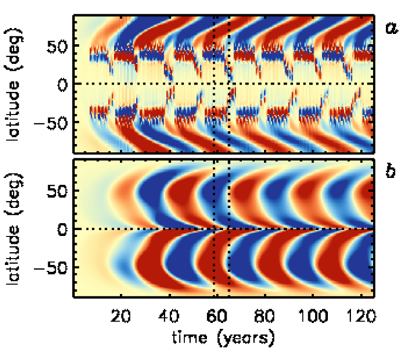
Figure 2.— Butterfly diagram for a representative solar dynamo simulation. ($a$) mean radial field $\left<B_{r}\right>$ at the surface ($r=R$) as a function of latitude and time. Blue and red denote inward and outward polarity respectively and the saturation level of the color table is $\pm$ 100 G. ($b$) Mean toroidal field $\left<B_{\phi}\right>$ near the base of the convection zone ($r=0.71R$; blue westward, red eastward, saturation $\pm 30kG$). Vertical lines denote times of 58.57, 58.83, and 64.94 yr represented in Fig. 3.

4. RESULTS AND DISCUSSIONS

Fig. 2 highlights magnetic cycles achieved in a solar dynamo simulation represented in terms of butterfly diagrams. Shown are the mean radial field near the surface (Fig. 2$a$) and the mean toroidal field near the base of the CZ (Fig. 2$b$) as a function of latitude and time. The numerical resolution of this simulation is 300$\times$512$\times$1024 in $r$, $\theta$, $\phi$ (maximum spherical harmonic degree 340) and the computation domain extends from $0.69R$–$R$, with an electrically conducting inner boundary and a radial field boundary condition on the outer surface.

The half-period of the magnetic cycle is roughly 11-12 yrs, comparable to the solar cycle. As in other advection-dominated 2D BL/FT models, this period is regulated largely by the imposed meridional flow and in particular the equatorward flow of several m s^-1 near the base of the CZ (Dikpati & Gilman, 2009; Charbonneau, 2010). Still, to our knowlege this is the first published demonstration of a self-sustained, cyclic solar dynamo model that incorporates a 3D flux emergence algorithm for the generation of poloidal field. The dynamo not only includes sunspots (BMRs), but as a BL model, it relies on them for its operation.

Fig. 3 shows an illustrative example of surface flux evolution. The sequence begins at $t=$ 58.57 yr ($a$) when a new sunspot pair has just emerged in the SH amid remnant flux from previous emergence events. Note also the slighly older spot pair in the NH at a latitude of about 45^∘ and longitude near -180^∘. About three months later ($b$), trailing flux from the southern spot (blue) has begun to disperse and merge with a growing axisymmetric band of negative flux at a latitude of roughly -65^∘. Similarly, trailing flux from the northern spot (red) contributes to a positive-polarity band of flux at a latitude of about 67^∘. About 6 years later ($c$), these bands (red in the north and blue in the south) have migrated toward higher latitudes and have begun to reverse the polar fields (see also Fig. 2$a$). Meanwhile, the next generation of sunspots has already begun to build opposite-polarity bands equatorward of these.

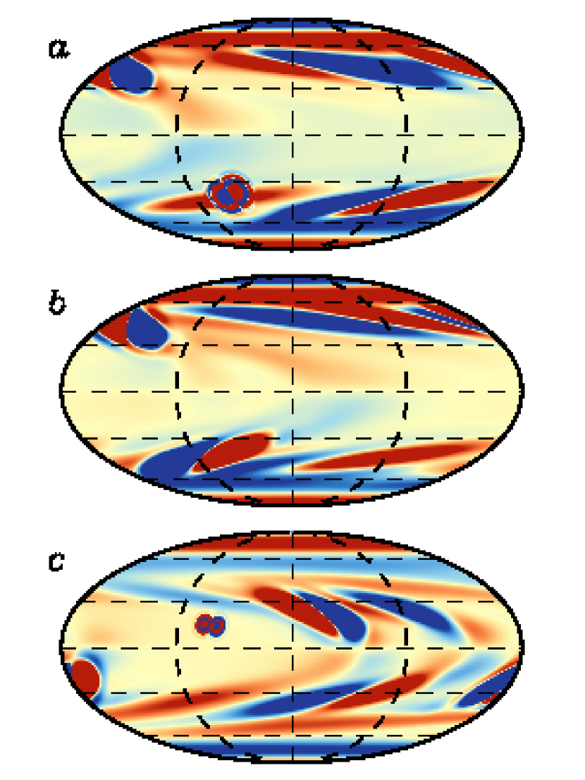
Figure 3.— Evolution of the radial magnetic field $B_{r}$ at the solar surface. Shown are Molleweide projections at the three times indicated by vertical lines in Fig. 2($a$), namely $t=$ 58.57, 58.83, and 64.94 yr. Blue and red denote inward (negative) and outward (positive) polarity with a saturation level of $\pm$ 100 G to highlight relatively weak fields. The low saturation level reveals some Gibbs ringing around the spots as a consequence of the spectral method, but this is two orders of magnitude smaller than the field at spot center (180 kG and 1.5 MG for the fresh spots in $a$ and $c$ respectively) and is quickly dissipated, with no significant contribution to the flux budget.

This surface flux evolution is similar to the evolution of magnetic flux as seen in photospheric magnetograms and as captured by SFT models and it demonstrates that the BL mechanism does indeed operate in a 3D context as originally envisioned by Babcock (1961) and Leighton (1964, 1969). The dispersal of tilted sunspot pairs due to differential rotation, meridional circulation, and turbulent diffusion generates a mean poloidal field that sustains the dynamo (see also YM13). Trailing flux from bipolar active regions migrates toward the poles from mid-latitudes in several streams (Fig. 2$a$) while leading flux cancels across the equator. Note that this cancellation occurs only in a time-integrated sense, since the randomness of spot appearances essentially guarantees that the 3D field distribution at any instant is not symmetric about the equator.

In many previous dynamo models, the mean toroidal field near the base of the CZ is taken as a proxy for the sunspot number. In our model this exhibits systematic equatorward propagation at low latitudes similar to the solar butterfly diagram (Fig. 2$b$). However, in our model this proxy is no longer necessary since we incorporate sunspots (BMRs) explicitly. Their behavior in Fig. 2$a$ does not agree as well with solar observations, showing a tendency to linger at mid-latitudes before a rapid rush toward the equator near the end of a cycle. This can largely be attributed to the masking function in eq. (3) which favors mid-latitudes. Since this masking function was originally designed to mimic Joy’s-law tilts that we capture explicitly, it will be justified to replace it with a more uniform low-latitude profile that may be calibrated to more closely match solar observations.

As mentioned in §3, field strengths in this preliminary model are artificially high due to the prodigious flux assigned to BMRs. Typical polar field strengths are 100 G, about an order of magnitude larger that solar values. However, the relative strengths are in reasonable agreement with solar observations in that most of the magnetic energy (ME) is in the mean toroidal field, which exceeds the ME in the non-axisymmteric field by a factor of 30-40 and the ME in the mean poloidal field by a factor of 3000-4000.

In summary, the main result of this letter is the construction of a viable 3D BL/FT solar dynamo model using a novel Spotmaker algorithm for flux emergence. Spotmaker is a 3D generalization of the double-ring algorithm previously used in 2D BL/FT models and provides a mechanism for unifying BL/FT dynamo models with SFT models, building on the sucesses of each. We focused here on the kinematic regime with imposed mean flows. Though this provides an instructive starting point, the real promise of this model will be realized when we consider nonlinear feedbacks and non-axisymmetric flows. By linking in the full ASH machinery to solve the anelastic equations of motion, we plan to include Lorentz-force feedbacks and enhanced radiative cooling in the vicinity of active regions. This should produce torsional oscillations as well as modulation of the meridional circulation and poloidal field generation over the course of multiple cycles. We will also consider more realistic sunspot distributions and alternative flux emergence algorithms such as that proposed by YM13. On a longer time scale, we will include resolved convective motions and investigate their role in the generation and transport of magnetic flux.

The model presented here is the first step toward a series of progressively more sophisticated and realistic 3D solar dynamo models that will allow us to study not only the physics of the dynamo itself, but also the response of the corona and heliosphere to cyclic dynamo-generated fields.

References

- Babcock (1961) Babcock, H. W. 1961, ApJ, 133, 572
- Baumann et al. (2006) Baumann, I., Schmitt, D., & Schüssler, M. 2006, A&A, 446, 307
- Brun (2010) Brun, A. S. 2010, EAS Pub. Ser., 44, 81
- Brun et al. (2004) Brun, A. S., Miesch, M. S., & Toomre, J. 2004, ApJ, 614, 1073
- Charbonneau (2010) Charbonneau, P. 2010, Living Reviews in Solar Physics, 7, http://www.livingreviews.org/lrsp-2010-3
- Choudhuri et al. (1995) Choudhuri, A. R., Schüssler, M., & Dikpati, M. 1995, Astron. Astrophys., 303, L29
- Clune et al. (1999) Clune, T. C., Elliott, J. R., Miesch, M. S., Toomre, J., & Glatzmaier, G. A. 1999, Parallel Computing, 25, 361
- Dikpati (2011) Dikpati, M. 2011, ApJ, 733, 90 (7 pp)
- Dikpati & Charbonneau (1999) Dikpati, M. & Charbonneau, P. 1999, ApJ, 518, 508
- Dikpati et al. (2004) Dikpati, M., de Toma, G., Gilman, P. A., Arge, C. N., & White, O. R. 2004, ApJ, 601, 1136
- Dikpati & Gilman (2007) Dikpati, M. & Gilman, P. A. 2007, Solar Phys., 241, 1
- Dikpati & Gilman (2009) —. 2009, Space Sci. Rev., 144, 67
- Durney (1997) Durney, B. R. 1997, ApJ, 486, 1065
- Guerrero et al. (2012) Guerrero, G., Rheinhardt, M., Brandenburg, A., & Dikpati, M. 2012, MNRAS, 420, L1
- Leighton (1964) Leighton, R. B. 1964, ApJ, 140, 1547
- Leighton (1969) —. 1969, ApJ, 156, 1
- Miesch (2005) Miesch, M. S. 2005, Living Reviews in Solar Physics, 2, http://www.livingreviews.org/lrsp-2005-1
- Munoz-Jaramillo et al. (2010) Munoz-Jaramillo, A., Nandy, D., P.C.H.Martens, & Yeates, A. R. 2010, ApJ, 720, L20
- Nandy & Choudhuri (2001) Nandy, D. & Choudhuri, A. R. 2001, ApJ, 551, 576
- Parfrey & Menou (2007) Parfrey, K. P. & Menou, K. 2007, ApJ, 667, L207
- Rempel (2006) Rempel, M. 2006, ApJ, 647, 662
- Schrijver (2001) Schrijver, C. J. 2001, ApJ, 547, 475
- Schüssler & Rempel (2005) Schüssler, M. & Rempel, M. 2005, A&A, 441, 337
- Stenflo & Kosovichev (2012) Stenflo, J. O. & Kosovichev, A. G. 2012, ApJ, 745, 129 (12pp)
- Wang & Sheeley (1991) Wang, Y. M. & Sheeley, N. R. 1991, ApJ, 375, 761
- Yeates & Munoz-Jaramillo (2013) Yeates, A. R. & Munoz-Jaramillo, A. 2013, MNRAS, 436, 3366