A class of compact entities in three component Bose - Einstein condensates.

Abstract

We introduce a new class of soliton-like entities in spinor three component BECs. These entities generalize well known solitons. For special values of coupling constants, the system considered is Completely Integrable and supports $N$ soliton solutions. The one-soliton solutions can be generalized to systems with different values of coupling constants. However, they no longer interact elastically. When two so generalized solitons collide, a spin component oscillation is observed in both emerging entities. We propose to call these newly found entities oscillatons. They propagate without dispersion and retain their character after collisions. We derived an exact mathematical model for oscillatons and showed that the well known one soliton solutions are a particular case.

I Introduction

The idea of spinor condensates was first suggested in seminal papers of Ho Shenoy+Ho:BinaryMixturesOfBEC and Ohmi Machida:BECWithInternalDoF ; Machida:SpinDomainInBEC . The experimental creation of spinor condensates Ketterle:OpticalConfinementOfBEC , in which the spin degree of freedom, frozen in magnetic traps, comes into play, opened the possibility to observe phenomena that are not present in single component Bose Einstein condensates. These include the formation of spin domains Ketterle:SpinDomainsInFroundStateOfBEC and spin textures Stamper-Kurn:SpinTextures . A theoretical description of the formation of spin domains can be found, for example in Tsubota:DomainFormationInBEC . A spinor condensate formed by atoms with spin $F$ is described by a macroscopic wave function with $2F+1$ components. Here we focus on the $F=1$ case, which has been studied in a number of theoretical works. The ground state structure was investigated by several authors, for instance in Ho:PhaseDiagramOfSpinorBEC ; Ho:GroundStateOfSpinorBEC ; Ueda:ExactEigenstatesOfSpinorBEC . Even multicomponent vector solitons with $F=1$ have been predicted; bright solitons in Wadati:SpinorSolitons , dark solitons Wadati:DarkSolitons , as well as gap solitons Malomed:SolitonsNonlinearModulation (the latter type requires the presence of an optical lattice).

We investigate the dynamics of an $F=1$ spinor Bose Einstein condensate for a wide range of scattering length. In particular, we address the general problem of spin soliton collisions. For one specific ratio of the scattering lengths, Wadati and coworkers in Wadati:BrightSpinorSolitons ; Wadati:KdV found a complete classification of the one soliton solution with respect to the spin states and even presented an explicit formula of the two-soliton solution. One soliton solutions come in two classes: polar, and ferromagnetic solitons Wadati:BrightSpinorSolitons ; Wadati:KdV . Both can be generalized to a wider set of scattering lengths. Here we consider all possible values of the ratio of scattering lengths. Our system is no longer integrable, but some of the one soliton solutions can be generalized to obtain solutions that preserve their shape throughout.

The paper is organized as follows: in chapter 2 we show that $F=1$ one soliton solutions can be generalized for arbitrary nonlinear coupling, we discuss their shape and collisions. In chapter 3 we introduce a new kind of soliton solutions, which we call oscillatons. We study their dynamics and interactions.

II General considerations

In this section we review and generalize results concerning the system of spinor Gross-Pitaevskii equations for the case of $F=1$ and equal coupling constants. This system is completely integrable and was thoroughly investigated by Wadati, Ieda and Miyakawa Wadati:BrightSpinorSolitons . Here we concentrate on bright soliton solutions.

To begin with, we consider a dilute gas of trapped bosonic atoms with hyperfine spin $F=1$. The wavefunction in vector form is $\mathbf{\Phi}\left(x,t\right)=\left(\Phi_{1},\Phi_{0},\Phi_{-1}\right)^{T}$ and it must satisfy the spinor Gross Pitaevski equation

$$\imath\hbar\partial_{t}\mathbf{\Phi}=\left[-\frac{\hbar^{2}}{2M}\partial_{x}^{2}+c_{0}\mathbf{\Phi}^{\dagger}\mathbf{\Phi}+c_{2}\left(\sum_{\alpha=1}^{3}\left(\mathbf{\Phi}^{\dagger}\hat{f}^{\alpha}\mathbf{\Phi}\right)\hat{f}^{\alpha}\right)\right]\mathbf{\Phi}.$$ (1)

Here $\hat{f}^{\alpha}(\alpha=1,2,3)$ are the angular momentum operators in 3x3 representation and $c_{0}$ is negative to allow for bright soliton formation.

In the paper of Ieda et al Wadati:BrightSpinorSolitons the authors considered this system with coupling constants $c_{2}=c_{0}\equiv c<0$. In this case Eq. (1) describes a completely integrable system. The authors find N soliton solutions via the Hirota method. In particular, they present both $\textrm{N}=1$ and $\textrm{N}=2$ solutions explicitly.

II.1 One soliton solutions

We introduce dimensionless units: $x\rightarrow\frac{\hbar^{2}\,L^{2}}{N|c_{0}|}\,x$ and $t\rightarrow\frac{2M}{\hbar}\left(\frac{\hbar^{2}\,L^{2}}{N|c_{0}|}\right)^{2}.$ Here $N$ is the number of atoms and $L$ is a characteristic length of the problem (e.g. $L=\sigma_{\perp}/\sqrt{3\pi}$ where $\sigma_{\perp}$ is the transverse size of trap confining the semi-one dimensional condensate). When we express Eq. (1) in these units, and divide the equation by $|c_{0}|$, all the coefficients but the ratio between self and cross nonlinear coupling $\frac{-c_{2}}{|c_{0}|}$, which we denote by $\gamma$, will be equal to one. To allow for the formation of bright solitons $c_{0}$ must be negative. The dimensionless form of our equation is

$$\imath\partial_{t}\mathbf{\Phi}=\Big{[}-\partial_{x}^{2}-\mathbf{\Phi}^{\dagger}\mathbf{\Phi}-\gamma\left(\mathbf{\Phi}^{\dagger}\hat{f}^{\alpha}\mathbf{\Phi}\right)\hat{f}^{\alpha}\Big{]}\mathbf{\Phi}.$$ (2)

When $\gamma=1$ the general one-soliton solution is given by

$$\mathbf{\Phi}=\frac{2ke^{\imath\varphi}}{1+\frac{1}{4k^{2}}e^{-2z}+k^{2}|\chi^{\dagger}\bar{\chi}|^{2}e^{2z}}\left[\frac{1}{2k}e^{-z}\chi+k(\chi^{\dagger}\bar{\chi})^{\ast}e^{z}\bar{\chi}\right],$$ (3)

where $z=k(x-x_{0}-2pt)$ a coordinate for observing soliton’s envelope moving with velocity $2p,$ $\varphi=px+(k^{2}-p^{2})t$ a coordinate for observing the soliton’ s carrier wave, $\chi=(\chi_{+1},\chi_{0},\chi_{-1})^{T}$ - the polarization of soliton (normalized spinor), and $\bar{\chi}=(\chi_{-1}^{\ast},-\chi_{0}^{\ast},\chi_{+1}^{\ast})^{T}$ - time reversed polarization.

The solitons can be classified according to the value of the parameter $\left|\chi^{\dagger}\bar{\chi}\right|=\left|\chi^{\dagger}\hat{T}\chi\right|\equiv\langle T\rangle$ the mean value of the time reversal operator. $\hat{T}$ is defined as $\hat{T}=e^{-\imath\pi\hat{f}^{y}}\,\hat{K},$ where $\hat{K}$ is a complex conjugate operator. $\langle T\rangle$ can take values ranging from $0$ to $1.$ Solutions with $\langle T\rangle$ taking extreme values are of the greatest interest to us, because they can be generalized to systems with general $\gamma.$ Solitons with intermediate values of $\langle T\rangle$ seem to be unique for integrable systems. We distinguish three classes of solitons
1. Ferromagnetic state
When $\langle T\rangle=0$ Eq.(3) simplifies into separable form

$$\mathbf{\Phi}=k\,\textrm{sech}\left[k(x-x_{0}^{\prime}-2pt)\right]e^{\imath px}e^{\imath(k^{2}-p^{2})t}\chi.$$ (4)

Furthermore, the condition $\chi^{\dagger}\bar{\chi}=0$ implies that $\chi$ can be written as

$$\chi^{(\textrm{ferro})}=e^{-\imath(\theta-\tau)}\left(\begin{array}[]{c}e^{-\imath\beta}\cos^{2}\frac{\alpha}{2}\\ \sqrt{2}\cos\frac{\alpha}{2}\sin\frac{\alpha}{2}\\ e^{\imath\beta}\sin^{2}\frac{\alpha}{2}\\ \end{array}\right)=e^{\imath\tau}\hat{\mathcal{U}}(\beta,\alpha,\theta)\left(\begin{array}[]{r}1\\ 0\\ 0\\ \end{array}\right).$$ (5)

This is the spin state which minimizes energy in a system of $c_{2}<0.$ This kind of solution can be generalized for any $\gamma\neq 1$. We do so by replacing $k$ multiplying the sech function in Eq. 5 with an appropriate $\gamma$ dependent coefficient. One can check that appropriate solution has the form

$$\mathbf{\Phi}^{(\textrm{ferro})}=\sqrt{\frac{2}{1+\gamma}}\,k\,\textrm{sech}\left[k(x-x_{0}-2pt)\right]e^{\imath p\,x}e^{\imath\left(k^{2}-p^{2}\right)t}\,e^{\imath\tau}\hat{\mathcal{U}}\,\left(\begin{array}[]{r}1\\ 0\\ 0\\ \end{array}\right).$$ (6)

We call it a generalized ferromagnetic soliton. The total number of atoms is

$$N_{\textrm{tot}}=\int_{-\infty}^{\infty}dx\,\mathbf{\Phi}^{\dagger}\mathbf{\Phi}=\frac{4}{1+\gamma}\,k,$$ (7)

the total mean spin

$$\mathbf{f}_{\textrm{tot}}=\int_{-\infty}^{\infty}dx\,\hat{\mathbf{e}}_{\alpha}(\mathbf{\Phi}^{\dagger}\hat{f}^{\alpha}\mathbf{\Phi})=N_{\textrm{tot}}\left(\begin{array}[]{c}\sin\alpha\cos\beta\\ \sin\alpha\sin\beta\\ \cos\alpha\\ \end{array}\right).$$ (8)

Here $\hat{\mathbf{e}}_{\alpha}$ are versors of the coordinate system ($\alpha=x,y,z,$ summation for repeating indices). Finally the total momentum and energy of the generalized ferromagnetic soliton are

$$P^{\textrm{ferro}}_{\textrm{tot}} = \int_{-\infty}^{\infty}dx\,\mathbf{\Phi}^{\dagger}(-\imath\partial_{x}\mathbf{\Phi})=N_{\textrm{tot}}\,p,$$ (9)

$$E^{\textrm{ferro}} = \int_{-\infty}^{\infty}dx\,\left[\partial_{x}\mathbf{\Phi}^{\dagger}\partial_{x}\mathbf{\Phi}-\frac{1}{2}(\mathbf{\Phi}^{\dagger}\mathbf{\Phi})^{2}-\frac{\gamma}{2}(\mathbf{\Phi}^{\dagger}\hat{f}^{\alpha}\mathbf{\Phi})(\mathbf{\Phi}^{\dagger}\hat{f}^{\alpha}\mathbf{\Phi})\right]=$$ (10)

$$= N_{\textrm{tot}}\left(p^{2}-\frac{N_{\textrm{tot}}^{2}(1+\gamma)^{2}}{48}\right).$$

2. The polar state
Considering Eq. (3) $\langle T\rangle=1$, we recover a normal sech-type soliton:

$$\mathbf{\Phi}=\sqrt{2}\,k\,\textrm{sech}\left[k(x-x_{0}-2pt)\right]e^{\imath px}e^{\imath(k^{2}-p^{2})t}\chi.$$ (11)

The constrain $\chi^{\dagger}\bar{\chi}=1$ implies that

$$\chi^{(\textrm{polar})}=e^{\imath\tau}\left(\begin{array}[]{c}-\frac{1}{\sqrt{2}}e^{-\imath\beta}\sin\alpha\\ \cos\alpha\\ \frac{1}{\sqrt{2}}e^{\imath\beta}\sin\alpha\\ \end{array}\right)=e^{\imath\tau}\hat{\mathcal{U}}(\beta,\alpha,\theta)\left(\begin{array}[]{r}0\\ 1\\ 0\\ \end{array}\right),$$ (12)

and one can check that the local mean spin density vanishes identically. Generalization of this soliton solution is straightforward. Since it is a spinless state, the spin mixing interaction term in Eq. (2) vanishes and what remains is stratified by (11) for all $\gamma.$ We will refer to this solution as ageneralized polar soliton

$$\mathbf{\Phi}^{(\textrm{polar})}=\sqrt{2}\,k\,\textrm{sech}\left[k(x-x_{0}-2pt)\right]e^{\imath p\,x}e^{\imath\left(k^{2}-p^{2}\right)t}e^{\imath\tau}\hat{\mathcal{U}}\left(\begin{array}[]{r}0\\ 1\\ 0\\ \end{array}\right).$$ (13)

Notice that the amplitude of the soliton is different from that of the ferromagnetic soliton, which leads to the different relation between the total number of atoms and parameter $k$

$$N_{\textrm{tot}}=4k.$$ (14)

The energy difference between ferromagnetic and polar solitons, with the same number of atoms, is:

$$E^{\textrm{ferro}}-E^{\textrm{polar}}=-\frac{1}{48}N_{\textrm{tot}}^{3}\gamma(2+\gamma).$$ (15)

3. Split solitons
If $0<\langle T\rangle<1,$ for every moment $t,$ each component of the local mean spin density vector $f^{\alpha}(x,t)=\mathbf{\Phi}^{\dagger}\hat{f}^{\alpha}\mathbf{\Phi},$ is an anisymmetric function of $x$ with respect to a certain point $x_{\textrm{node}}(t).$

This implies that the total mean spin of this state, $\mathbf{f}_{\textrm{tot}}=\int dx\,\mathbf{f}(x),$ is equal to $0.$ Careful examination of the density profile of this kind of soliton reveals the reason for this. For $\langle T\rangle$ close to $0$ the density splits into two disjointed peaks traveling with the same velocity. Each of these peaks is actually a ferromagnetic soliton with mean spins anti parallel to each other. As $\langle T\rangle$ approaches $1$ the peaks begin to merge, consequently creating a single entity without spin - a polar soliton. Figure (1) shows the density profile $n(x)=\mathbf{\Phi}^{\dagger}\mathbf{\Phi},$ of split soliton for different values of $\langle T\rangle$ and $\gamma=1$ from Eq. (3).

Figure 1: Density profiles ($n(x)=\mathbf{\Phi}^{\dagger}\mathbf{\Phi}$) of split solitons for different values of $\langle T\rangle$, $\gamma=1$.

II.2 Collisions

II.2.1 Elastic Collisions

We begin with a short review of the integrable case. The only effect of a two soliton collision in the case of scalar solitons is a phase shift. The wave function after the collision can acquire additional phase and translation ($\mathbf{\Phi}\rightarrow e^{\imath\tau}\mathbf{\Phi},$ and $\mathbf{\Phi}(x,t)\rightarrow\mathbf{\Phi}(x-\Delta x,t).$) Ablowitz+Segur:Solitons+InverseScattering . In the context of the analysis of the previous section we can distinguish the following cases:
(a) Polar-polar solitons collisions In a polar-polar soliton collision, the solitons emerge unaltered, aside from phase changes. It is the result of the general rule: polar soliton cannot change polarization of it’s partner.
(b) Ferromagnetic-ferromagnetic solitons collisions Ferromagnetic solitons change their phases and can rotate each other’s polarization. However, the values of $\langle T\rangle$ of each of the solitons remain equal to $0$; in this kind of collision, solitons can’t change their type.
(c) Polar-ferromagnetic solitons collision In a collision, ferromagnetic solitons experience only phase shifts; polarizations remain unchanged. This is a consequence of the inability of a polar soliton to influence the polarizations of other solitons when they interact. In the case of a polar soliton, a combination of phase shifts and polarization rotation can change $\langle T\rangle.$ This means that a polar soliton can be transformed into a split soliton in the collision. However, $\langle T\rangle$ can never reach $0,$ because the total spin must be conserved and there is no spin transfer in the collision. A polar soliton will not change into a split soliton if the polarizations of ferromagnetic and polar solitons are orthogonal: $\chi^{(\textrm{polar})\dagger}\chi^{(\textrm{ferro})}=0.$

II.2.2 Generalized soliton collisions

Previously we have seen that two classes of one-soliton solutions can be generalized to (almost) arbitrary $\gamma$. However, in order to call these solutions real solitons one has to examine their mutual interactions. We have conducted a series of numerical experiments on collisions of generalized solitons for various values of $\gamma.$ We discovered that non-dissipating, localized entities emerge in the wake of the collision. Although those entities resemble solitons, there is a major difference: they are no longer stationary - populations of magnetic components are oscillating with a well defined frequency. This behavior is generic, it occurs for almost all values of $\gamma$ (with exceptions of $\gamma=1$, when system is integrable and $\gamma=0$, when there are no spin mixing interactions) and all configurations of collisions. We propose to call these oscillating, soliton-like entities oscillatons. The creation of oscillatons is indeed generic, however, depending on the details of the collisions (such as the sign of $\gamma$ and classes of solitons participating in it) this process can be accompanied by some side effects (for example: a short period of intense radiation, a small momentum transfer).

We consider a head-on collision of two generalized solitons for some $\gamma.$ At $t=0$, when solitons are far apart, the wave function is, within a good approximation, a sum of two one-soliton wave functions $\mathbf{\Phi}(t=0)\approx\mathbf{\Phi}^{(1)}+\mathbf{\Phi}^{(2)}$. The wave functions of solitons $\mathbf{\Phi}^{(i)}$ are given by (6) for generalized ferromagnetic solitons and (13) for generalized polar solitons.

Each of the participating solitons is described by a set of parameters: gauge phase $\tau$, Euler angles $\beta,\alpha$ and $\theta$ (in the case of a polar soliton $\theta$ is a dummy variable), momentum $p$ and amplitude $k.$ In principle, the result of a collision can depend on all of these parameters. However, Galilean and gauge-rotation invariance of the equation reduces the number of parameters significantly. Firstly, the Galilean invariance allows us to fix one of the solitons in place (we will call it the target) and set the other one in motion (we will call it the bullet). Equivalently, the collision can be viewed in the reference frame moving with the target soliton. Secondly, gauge-rotation invariance allows us to fix the target’s polarization to “standard” orientation ($(1,0,0)^{T}$ for the ferromagnetic and $(0,1,0)^{T}$ for the polar target) and the gauge phase of the target can be set to zero. In this work we restricted considerations to equal norms. This configuration allows for observation of the behavior of a post-target oscillaton at large times. As an example we will use a polar-ferromagnetic collision (for polar-polar collision see MyPRL:Oscillatons ).

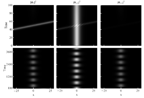
Figure 2: Top: Density plot of $|\Phi_{1}|^{2}$ (left), $|\Phi_{0}|^{2}$ (center) and $|\Phi_{-1}|^{2}$ (right) for a collision of a stationary polar and a moving ferromagnetic soliton. Here $\gamma=-1/3,$ the momentum is $p=1.5,$ and the Euler angles are $\beta=\alpha=\pi/4,$ $\tau=\theta=0.$ Both solitons are normalized to $1.$ Bottom: Details of the initially stationary polar soliton pictured after the collision and to a much longer time scale. Observe the oscillatory character of the wave function components.

Figures (2) show space-time plots of collisions and propagation of post-target oscillatons in a time scale much longer then the time of collision. The oscillatory behavior can be clearly seen. Each of those components can be fitted with the function $f_{m}(t)=a_{m}+b_{m}\,\cos(\omega t+\varphi_{m}),$ where $m=1,0,-1.$ Relative phases between components are such, that the total density $|\Phi_{1}(x_{\textrm{max}})|^{2}+|\Phi_{0}(x_{\textrm{max}})|^{2}+|\Phi_{-1}(x_{\textrm{max}})|^{2}$ is constant in time. The frequency $\omega$ defines the frequency of an oscillaton.

An important feature of the collision is the spin transfer. Figures (3) show space-time density plot of local spin density $|\mathbf{f}(x,t)|=\sqrt{(\mathbf{\Phi}^{\dagger}\hat{f}^{\alpha}\mathbf{\Phi})(\mathbf{\Phi}^{\dagger}\hat{f}^{\alpha}\mathbf{\Phi})}.$ At first, only a ferromagnetic soliton has spin. During the collision, a polar soliton, and hence a post-polar oscillaton, acquire some spin at the expense of a post-ferro oscillaton. Spin densities of both oscillatons are constant and the total spin ($|\mathbf{f}_{\textrm{tot}}|=\int dx|\mathbf{f}(x,t)|$) is conserved. In the case of polar-polar collision, both participants start with no spin. During the collision, both target and bullet acquire spins, but the spin vectors are anti parallel, so that the total spin is still $0.$

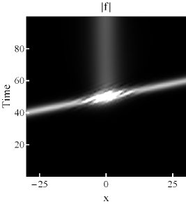
Figure 3: Density plot of local spin density $|\mathbf{f}(x,t)|$ for the collision showed in Fig. (2).

We found that the oscillation frequency is determined by the spin transferred in the collision. It depends only on the magnitude of the spin vector, not its direction: the greater the spin transfer, the greater the oscillation frequency. The amount of spin transferred in the collision depends on all collision parameters: the momentum $p$, Euler angles, norm and $\gamma.$

Dependance on momentum is mostly due to the time of interaction; fast collision means less time for atoms to transfer and weaker effects of interactions. We found that the frequency of oscillations depends on the momentum as $\omega(p)\propto e^{-a\,p}/p^{b},$ where $a$ and $b$ are constants, fitted for a particular collision type. Notice that $\omega$ has a maximum for some $p.$ The collisions are elastic (oscillatons are not created) when spinors of participating solitons ($\chi$ in Eq. (13) and Eq. (6)) are parallel or perpendicular. In the case of parallel spinors, the equations effectively reduce to the scalar Gross-Pitaevskii equation, which is integrable, hence, the collision is elastic.

Another noteworthy feature of the dynamics of the collisions is the very small momentum transfer. Notice that despite a very long time of observation, the oscillaton practically has not moved from its original position (aside from a small “recoil”, characteristic of polar-ferro soliton collision  Wadati:BrightSpinorSolitons . This means that the only effective way to transfer energy between solitons/oscillatons is a transfer and redistribution of atoms between magnetic components.

The collisions between generalized solitons are inelastic. As soon as oscillatons split up, we observe a short period of intense radiation. The actual intensity of this radiation strongly depends on the collision setup and value of $\gamma.$ Figure (4) shows norms of oscillaton as a function of time.

Figure 4: Norm $\int\mathbf{\Phi}^{\dagger}\mathbf{\Phi}\,dx$ of the Oscillatons created in collision of polar and ferromagnetic soliton as a function of time and $\gamma.$ Collision setups are as in Fig. (2). Atoms are lost due to radiation.

Note the exponential-like norm decay to some fixed value, this atom loss is due to radiation. In the collision solitons and/or oscillatons exchange atoms. This leads to the spin and energy transfer. It seems that, in the collision, solitons can acquire an extra amount of atoms and end up in a non stable state. By releasing these excess particles, in the form of radiation, the oscillaton may transfer into its equilibrium state. The frequency of oscillations is insensitive to radiation.

III A new type of soliton: an oscillaton

III.1 One oscillaton solution

In a collision of solitons, spin is transferred such that the spin vector of the outgoing oscillaton has a non-zero component in the $XY$ plane. The amplitude of oscillations can be affected by rotating the frame of reference, the frequency of oscillations however does not change. Particularly, in a reference frames where the projection of the spin vector on the Z-axis was greater, the amplitude of oscillations dropped. In a special frame, in which spin vector is parallel to $Z$-axis, the amplitude is $0.$ On top of that, an oscillaton has a very simple form when viewed in this “good” reference frame: a $m=0$ component vanishes, $m=\pm 1$ have constant modulai with time dependence in the form of a linear phases increase. In summary, an oscillaton wave function can be modeled by the following anzats

$$\mathbf{\Phi}=e^{\imath\tau}\hat{\mathcal{U}}(\beta,\alpha,\theta)\left[\eta_{+}(x)e^{\imath\mu_{+}t}\left(\begin{array}[]{r}1\\ 0\\ 0\\ \end{array}\right)+\eta_{-}(x)e^{\imath\mu_{-}t}\left(\begin{array}[]{r}0\\ 0\\ -1\\ \end{array}\right)\right],$$ (16)

where $\eta_{\pm}$ are real, symmetric functions, $\mu_{\pm}$ are positive, real numbers and $\hat{\mathcal{U}}$ is a spin rotation operator parameterized by the Euler angles $\{\beta,\alpha,\theta\}.$ This anzats describes oscillations of component populations, as can be seen by examining the modulai of components

$$|\Phi_{0}|^{2} = \frac{1}{2}\sin^{2}\alpha\left(\eta_{+}^{2}+\eta_{-}^{2}+2\eta_{+}\eta_{-}\cos\left[\omega\,t-2\theta\right]\right),$$ (17)

$$|\Phi_{\pm 1}|^{2} = \eta_{\pm}^{2}\sin^{4}\frac{\alpha}{2}+\eta_{\mp}^{2}\cos^{4}\frac{\alpha}{2}-\frac{1}{2}\eta_{+}\eta_{-}\sin^{2}\alpha\cos\left[\omega\,t-2\theta\right],$$ (18)

where $\omega\equiv\mu_{+}-\mu_{-}.$ The local spin density in this state is

$$\mathbf{f}=\hat{e}_{\alpha}(\mathbf{\Phi}^{\dagger}\hat{f}^{\alpha}\mathbf{\Phi})=\left(\eta_{+}^{2}-\eta_{-}^{2}\right)\left(\begin{array}[]{c}\sin\alpha\cos\beta\\ \sin\alpha\sin\beta\\ \cos\alpha\\ \end{array}\right).$$ (19)

We find that the $\beta$ angle plays a role only in determining the orientation of the spin vector. We also find that the total spin is constant in time.

The total density profile of oscillaton is constant in time

$$n=\mathbf{\Phi}^{\dagger}\mathbf{\Phi}=\eta_{+}^{2}+\eta_{-}^{2}.$$ (20)

This anzats substituted into Eq. (2) leads to the following system of two coupled ordinary differential equations

$$-\mu_{\pm}+(1+\gamma)\eta_{\pm}^{2}+(1-\gamma)\eta_{\mp}^{2}+\frac{\eta_{\pm}^{\prime\prime}}{\eta_{\pm}}=0.$$ (21)

The problem has thus been reduced to solving ordinary differential equations. Additionally we have a first integral

$$-\mu_{+}\eta_{+}^{2}-\mu_{-}\eta_{-}^{2}+\frac{1+\gamma}{2}\left(\eta_{+}^{4}+\eta_{-}^{4}\right)+(1-\gamma)\eta_{+}^{2}\eta_{-}^{2}+\eta_{+}^{\prime 2}+\eta_{-}^{\prime 2}=\textrm{const}$$ (22)

The equations (21) are nonlinear, so amplitudes of wave function components $\eta_{\pm}$ determine chemical potentials $\mu_{\pm},$ and $\omega=\mu_{+}-\mu_{-}.$ For the case of $\mu_{+}=\mu_{-}\equiv\mu$ (or $\omega=0$) we have no oscillations. This implies $\eta_{+}=\eta_{-}=\sqrt{\mu}\,\textrm{sech}(\sqrt{\mu}x)$ and the spinor part of the wavefunction is proportional to $(1,0,-1)^{T},$. This can be obtained from polar spinor $(0,1,0)^{T}$ by a rotation $\hat{\mathcal{U}}.$ Hence that polar soliton (13) is a special case of an oscillaton. When $\mu_{-}=0$ or $\mu_{+}=0$ the ferromagnetic soliton (6) is obtained from Eq. (21). Again, we see that a ferromagnetic soliton is also a special case of an oscillaton.

This ansatz opens new possibilities of finding both exact and approximate solutions. A particular case is when $\gamma=1$ (integrable system), for which a solution for the pair of equations (21) is obtained explicitly. For this $\gamma$ the equations for $\eta_{\pm}$ decouple and each can be solved analytically. The solutions of interest are

$$\eta_{\pm}(x)=\sqrt{\mu_{\pm}}\,\textrm{sech}\left(\sqrt{\mu_{\pm}}\,x\right).$$ (23)

We have found a solution that looks like being composed of two ferromagnetic solitons! As long as $\mu_{+}\neq\mu_{-}$ there will be oscillations with frequency $\omega=\mu_{+}-\mu_{-},$ although, it is not possible to obtain such an oscillaton in a collision.

In order to ascribe an oscillaton as obtained in a particular collision, one has to follow the steps listed below.

1. Establish the orientation of the spin vector of the oscillaton and perform a rotation to the reference frame in which this vector will be parallel to the $Z$-axis We will call this frame of reference the eigenframe.

2. Determine the chemical potentials, the $\mu_{\pm}$ of $m=\pm 1$ components of the wave function.

3. Insert the chemical potentials into the oscillaton equations (21) and solve them for $\eta_{+}$ and $\eta_{-}$.

The first two steps can always be completed. The third is problematic. In general, the oscillaton equations (21) are not exactly solvable. However, in the following sections we will show that, in the cases of oscillatons created in collisions of generalized polar and ferromagnetic solitons, approximate solutions can indeed be found.

III.1.1 Post-ferromagnetic oscillaton

Figure (5) shows an oscillaton “created” out of a ferromagnetic soliton in polar-ferro collision, when viewed in its eigenframe. In this collision $\gamma=-1/3,$ the ferromagnetic soliton was the target and the polar soliton with $p=1.5,$ $\alpha=\beta=\pi/4,$ $\tau=\theta=0,$ was the bullet.

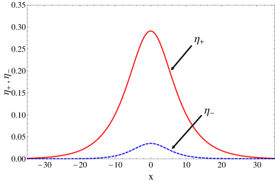
Figure 5: (Color online) Modulus of components of post-ferromagnetic oscillaton viewed in its eigenframe: $|\Phi_{1}|=\eta_{+}$ (red, solid line) and $|\Phi_{-1}|=\eta_{-}$ (blue , dashed line). The oscillaton was created in a collision of the target ferromagnetic soliton and the bullet polar soliton with $p=1.5,$ $\alpha=\beta=\pi/4,$ $\tau=\theta=0,$ and $\gamma=-1/3.$

Looking back to Fig. (5), it is clear that one of the components of the wave function is much smaller then the other, or $\eta_{+}\gg\eta_{-}.$ In terms of our equations (21) this means that we can neglect $\eta_{-}^{2}$ terms in comparison to $\eta_{+}^{2}$

$$-\mu_{+}+(1+\gamma)\eta_{+}^{2}+\frac{\eta_{+}^{\prime\prime}}{\eta_{+}} \approx 0$$ (24)

$$-\mu_{-}+(1-\gamma)\eta_{+}^{2}+\frac{\eta_{-}^{\prime\prime}}{\eta_{-}} \approx 0.$$ (25)

Now, the first equation depends only on $\eta_{+}$ and can be solved exactly: $\eta_{+}=\sqrt{2\mu_{+}/(1+\gamma)}\,\textrm{sech}\left(\sqrt{\mu_{+}}\,x\right).$ We next insert this value into the equation for $\eta_{-}$, where it plays the role of a trapping potential:

$$\eta_{-}^{\prime\prime}+\left[-\mu_{-}+2\mu_{+}\left(\frac{1-\gamma}{1+\gamma}\right)\textrm{sech}^{2}\left(\sqrt{\mu_{+}}\,x\right)\right]\eta_{-}=0.$$ (26)

Fortunately, this equation can be solved exactly Landau+Lifshitz:vol3 . The even solution is

$$\eta_{-}\propto\textrm{sech}^{\epsilon}\left(\sqrt{\mu_{+}}\,x\right)\,P^{(\epsilon,\epsilon)}_{2n}\left[\textrm{tanh}\left(\sqrt{\mu_{+}}\,x\right)\right],$$ (27)

where $\epsilon=\sqrt{\mu_{-}/\mu_{+}},$ $n=0,1,2,\ldots$ and $P^{(a,b)}_{m}\left[z\right]$ is a Jacobi polynomial, given by

$$P^{(a,b)}_{m}\left[z\right]=\frac{(-1)^{m}}{2^{m}m!}(1+z)^{-a}(1-z)^{-b}\frac{d^{m}}{dz^{m}}(1+z)^{a+m}(1-z)^{b+m}.$$ (28)

The first two solutions are

$$\eta_{-}^{(n=0)} \propto \textrm{sech}^{\epsilon}\left(\sqrt{\mu_{+}}\,x\right),$$

$$\eta_{-}^{(n=1)} \propto \textrm{sech}^{\epsilon}\left(\sqrt{\mu_{+}}\,x\right)\left[1-\left(\frac{1+2\epsilon}{2+2\epsilon}\right)\textrm{sech}^{2}\left(\sqrt{\mu_{+}}\,x\right)\right].$$

Equation (26) imposes a quantization condition on the chemical potential $\mu_{-}$:

$$\mu_{-}=\frac{\mu_{+}}{4}\left[-1-4n+\sqrt{1+8\frac{1-\gamma}{1+\gamma}}\right]^{2}.$$ (29)

The condition $\mu_{-}\geq 0$ ($\eta_{-}$ must be a bounded state) gives the number of allowed energy levels $n.$ For $\gamma>-1/2$ there is only one eigenvalue, corresponding to $n=0.$ As $\gamma$ approaches $-1/2$ from above the $n=1$ value appears. At $\gamma=-9/11,$ $n=2$ appears. As we near $\gamma=-1,$ the spectrum becomes arbitrarily rich. Unfortunately, for $\gamma\rightarrow-1$ our approximation breaks down, as can be seen from Eq. (24). Luckily, from the physical point of view, the most interesting cases are for $\gamma\sim 0,$ where the approximation should work.

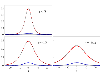
Figure 6: Comparison of solutions of Eq. (24) and (25) with post-ferromagnetic oscillatons found numerically viewed in their respective eigenframes. Oscillatons have been created in the collision of a target ferromagnetic soliton and a bullet polar soliton with $p=1.5,$ $\alpha=\beta=\pi/4,$ $\tau=\theta=0.$ The collisions were carried out for three cases of $\gamma:$ $1/3$ (top-left panel), $-1/3$ (bottom-left panel) and $-7/12$ (bottom-right panel). Agreement between the approximate solution for $\eta_{\pm}$ (lines) and red/blue dots obtained in the simulation is very good. In order to obtain the solutions the chemical potentials $\mu_{\pm}$ and the normalization constant of $\eta_{-}$ had to be fitted to match the numerical results. For all presented cases $n$ in Eq. (29) has been found to be $0.$

Figure (6) shows a comparison between solutions of approximate equations (24), (25) and post-ferromagnetic oscillatons obtained in ferro-polar soliton collisions for different values of $\gamma.$ In all cases the $\eta_{-}$ component ended up in the ground state ($n=0$ in Eq. (29)), even for $\gamma=-7/12<-1/2.$ Agreement between the model and the results of numerical simulations is very good.

III.1.2 Post-polar Oscillaton

Figure (7) compares components of the wavefunction of a post-polar oscillaton viewed in its eigenframe and the original polar soliton. Here we use as an example the collision setup presented in Fig. (2).

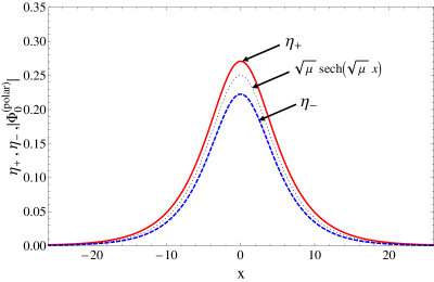
Figure 7: (Color online) Modulus of components of post-polar oscillaton viewed in its eigenframe: $|\Phi_{1}|=\eta_{+}$ (red,solid line) and $|\Phi_{-1}|=\eta_{-}$ (blue, dashed line). Components are compared with $\sqrt{\mu}\,\textrm{sech}(\sqrt{\mu}\,x)$ (dotted line). The oscillaton was created in the collision of the target polar soliton and the bullet ferromagnetic soliton with $p=1.5,$ $\alpha=\beta=\pi/4,$ $\tau=\theta=0,$ and $\gamma=-1/3.$

In this case, $\eta_{+}$ and $\eta_{-}$ are comparable. We propose the following ansatz:

$$\eta_{\pm}=\alpha_{\pm}\,\textrm{sech}^{\sqrt{\mu_{\pm}/\mu}}\left(\sqrt{\mu}\,x\right),$$ (30)

where $\mu$ is some “central” chemical potential. We anticipate that the central chemical potential is in fact the amplitude $\mu=k^{2}$ of the initial polar soliton (see Eq. (13)). This was confirmed by numerical simulations. Now, we will assume that the exponents in (30) can be written in the following form

$$\sqrt{\frac{\mu_{\pm}}{\mu}}\equiv\sqrt{1+\delta_{\pm}},$$ (31)

where $\delta_{\pm}$ are small corrections. Ansatz (30) inserted into equations (21) leads to the following system

$$(1+\gamma)\alpha_{\pm}^{2}\textrm{sech}^{2\sqrt{1+\delta_{\pm}}}\left(\sqrt{\mu}\,x\right)+$$

$$+(1-\gamma)\alpha_{\mp}^{2}\textrm{sech}^{2\sqrt{1+\delta_{\mp}}}\left(\sqrt{\mu}\,x\right)+$$

$$-\mu_{\pm}\left(1+\frac{1}{\sqrt{1+\delta_{\pm}}}\right)\textrm{sech}^{2}\left(\sqrt{\mu}\,x\right)=0.$$ (32)

In order to make further progress with equation (III.1.2) we investigate the Taylor expansion of $\textrm{sech}^{2\sqrt{1+\delta}}$ in $\delta$

$$\textrm{sech}^{2\sqrt{1+\delta}}\left(\sqrt{\mu}\,x\right) = \textrm{sech}^{2}\left(\sqrt{\mu}\,x\right)+\left(\frac{d}{d\delta}\,\textrm{sech}^{2\sqrt{1+\delta}}\right)\Big{|}_{\delta=0}\,\delta+\ldots=$$ (33)

$$= \textrm{sech}^{2}\left(\sqrt{\mu}\,x\right)\left[1+\delta\,\ln\left(\textrm{sech}\left(\sqrt{\mu}\,x\right)\right)\right]+\ldots$$

For $|x|\lesssim 1/\sqrt{\mu},$ the second term in the expansion can be neglected. Within this region of $x,$ $\textrm{sech}^{2\sqrt{1+\delta}}\approx\textrm{sech}^{2}$ and equation (III.1.2) can be satisfied, as long as

$$\mu_{\pm}+\sqrt{\mu}\,\sqrt{\mu_{\pm}}=(1+\gamma)\alpha_{\pm}^{2}+(1-\gamma)\alpha_{\mp}^{2}.$$ (34)

(since $1+\delta_{\pm}=\mu_{\pm}/\mu$). This relation is valid as long as we can approximate $\textrm{sech}^{2\sqrt{1+\delta}}$ by $\textrm{sech}^{2}$ in equation (III.1.2). It is easy to see that this approximation will work for $|x|\gg 1/\sqrt{\mu}.$ For large $x,$ $\textrm{sech}^{2\sqrt{\mu_{\pm}/\mu}}$ terms can be dropped and Eq. (21) reduces to

$$-\mu_{\pm}+\frac{\eta_{\pm}^{\prime\prime}}{\eta_{\pm}}=0,$$ (35)

satisfied by ansatz (30), as $\alpha_{\pm}\textrm{sech}^{\sqrt{\mu_{\pm}/\mu}}(\sqrt{\mu}\,x)\rightarrow 2\alpha_{\pm}\exp\left(-\sqrt{\mu}|x|\right),$ when $|x|\gg 1\/\sqrt{\mu}.$

Now we will establish validity of our approximation in the intermediate range of $x,$ i.e. $|x|\gtrsim 1/\sqrt{\mu}.$ So far we haven’t used the fact that $\delta_{\pm}$ should be small. For small $\delta$ and $|x|\gtrsim 1\sqrt{\mu}$ the expansion (33) can be written as

$$\textrm{sech}^{2\sqrt{1+\delta}}\left(\sqrt{\mu}\,x\right) = \textrm{sech}^{2}\left(\sqrt{\mu}\,x\right)\Bigg{[}1+\delta\ln\left(\textrm{sech}\right)+.$$ (36)

$$+\delta^{2}\left(-\frac{1}{4}\ln(\textrm{sech})+\frac{1}{2}\ln^{2}(\textrm{sech})\right)+\ldots\Bigg{]}$$

$$\approx \textrm{sech}^{2}(\sqrt{\mu}\,x)\left[1+\delta\sqrt{\mu}\,|x|+\frac{1}{2}\left(\delta\sqrt{\mu}\,|x|\right)^{2}+\ldots\right]$$

$$= \textrm{sech}^{2}\left(\sqrt{\mu}\,x\right)\,e^{\delta\sqrt{\mu}\,|x|}.$$

This means, that $\textrm{sech}^{2\sqrt{1+\delta}}\approx\textrm{sech}^{2},$ if $|x|\ll 1/\delta\sqrt{\mu}$ and we conclude, that our approximation is valid everywhere if $1\/\sqrt{\mu}\ll 1/\delta\sqrt{\mu},$ or $\delta\ll 1.$ In order to convince ourself that $\delta_{\pm}$ are indeed small, we perform an estimate using Eq. (34). As we saw in Fig. (7) amplitudes of oscillaton components differ by small corrections from the amplitude of the initial polar soliton. Knowing this, we can write $\alpha_{\pm}^{2}=\mu(1\pm\Delta)$, where $\mu$ is an amplitude of the initial soliton and $\Delta$ is small. Inserting it into equations (34) we get

$$\left(\sqrt{1+\delta_{\pm}}\right)^{2}+\sqrt{1+\delta_{\pm}}=2\left(1\pm\gamma\,\Delta\right).$$ (37)

The solution to this equation is $\delta_{\pm}\approx\pm\frac{4}{3}\gamma\,\Delta$.

We see that, indeed, small differences in amplitudes implies small differences in chemical potentials. For an alternative calculations see Appendix A.

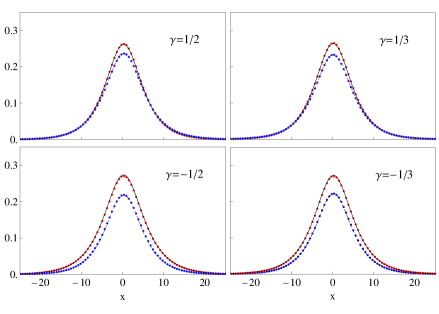
Figure 8: Comparison of approximate solutions (30) and (III.1.2) with post-polar oscillatons found numerically viewed in their respective eigenframes. oscillatons have been created in a collision of the target polar soliton and the bullet ferromagnetic soliton with $p=1.5,$ $\alpha=\beta=\pi/4,$ $\tau=\theta=0.$ The collisions were carried out for four cases of $\gamma:$ $1/2$ (top-left panel), $1/3$ (top-right panel), $-1/2$ (bottom-left panel) and $-1/3$ (bottom-right panel). Agreement between approximate solution for $\eta_{\pm}$ (solid/dashed line) and red/blue dots obtained in simulation is very good. In order to obtain the solutions, chemical potentials $\mu_{\pm}$ had to be fitted to mach the numerical results. The central chemical potential $\mu$ in Eq. (30) and (III.1.2) is found to be the amplitude of initial polar soliton $\mu=k^{2}$ (see Eq. (13)).

Figure (8) presents a comparison of approximate solutions (30) and (III.1.2) with post-polar oscillatons obtained in polar-ferro solitons collisions for different values of $\gamma.$ The agreement between the model and numerical results, for all $x,$ is very good.

III.2 Oscillaton collisions

The results of numerical experiments show that there is no qualitative difference between oscillatons and generalized solitons. We observe the same characteristic features: spin transfer, brief periods of radiation, small momentum transfer and so on. After the collision, oscillatons emerge altered, but nevertheless still described by our model. Besides a small atomic loss due to radiation and a tiny momentum change, oscillatons change their frequency of oscillations. Evidently, this is the result of spin transfer during the collision - a mechanism we discussed above. The similarity between solitons and oscillatons collisions is no surprise. Our previous considerations showed that both polar and ferromagnetic solitons are indeed special cases of oscillatons - non oscillating ones. In Table 1 we compare oscillaton parameters before and after a collision. We choose to look at changes in crucial parameters: chemical potentials $\mu_{\pm}$, total spin $\mathbf{f}_{\textrm{tot}}$. We analyze four cases. First we consider post-polar vs post-polar oscillaton collision for (A) $\gamma=-1/3$, and (B) $\gamma=1/3$. We collide an oscillaton with small spin (I) with one of much larger spin (II). From the point of view of the oscillaton with greater spin, the collision was almost elastic; the relative change of chemical potentials $\mu_{\pm}$ and spins are very small. This behavior is somewhat similar to the elastic collision of two ferromagnetic solitons in the case of a completely integrable system ($\gamma=1$), when the solitons, due to interaction, only rotate each other’s spins. On the other hand, the oscillaton with smaller spin experiences not only a rotation of its spin vector, but also a substantial increase of its magnitude.

Next we consider the collision of post-polar and post-ferromagnetic oscillatons for (C) $\gamma=-1/3$ and (D) $\gamma=1/3$. The results are analogous. Post ferromagnetic oscillatons (labeled as II), with greater spin, collide almost elastically: chemical potentials and spins have hardly changed. The post-polar oscillatons (I), with smaller spin, similarly to the previous case, experiences not only reorientation of the spin vector, but also an increase of magnitude.

Table 1: Comparison of the oscillaton parameters before and after collision. Here we define $|\mathbf{f}_{\textrm{tot}}|\equiv\int|\mathbf{f}^{(\textrm{before})}|\textrm{d}x$, $\Delta\mu_{\pm}\equiv\frac{\mu_{\pm}^{(\textrm{after})}-\mu_{\pm}^{(\textrm{before})}}{\mu_{\pm}^{(\textrm{before})}}$, $\Delta|\mathbf{f}_{\textrm{tot}}|\equiv\frac{\int|\mathbf{f}^{(\textrm{after})}|-|\mathbf{f}^{(\textrm{before})}|\textrm{d}x}{\int|\mathbf{f}^{(\textrm{before})}|\textrm{d}x}$, $\cos\Delta\theta\equiv\frac{\mathbf{f}^{(\textrm{before})}\cdot\mathbf{f}^{(\textrm{after})}}{|\mathbf{f}^{(\textrm{before})}||\mathbf{f}^{(\textrm{after})}|}$

	$|\mathbf{f}_{\textrm{tot}}|$	$\Delta\mu_{+}$	$\Delta\mu_{-}$	$\Delta|\mathbf{f}_{\textrm{tot}}|$	$\cos\Delta\theta$
A	Post—polar vs. post—polar oscillaton collision at $\gamma=-1/3$
I	0.05535	-0.09035	0.06098	3.325	0.9844
II	0.2175	0.002253	-0.002147	-0.02487	-0.1902
B	Post—polar vs. post—polar oscillaton collision at $\gamma=1/3$
I	0.0279	0.1021	-0.08473	6.947	0.822
II	0.1106	-0.007527	0.004616	-0.1147	-0.733
C	Post—polar vs. post—ferro oscillaton collision at $\gamma=-1/3$
I	0.05535	-0.06036	0.04176	-0.445	0.7197
II	0.977	0.0004905	-0.0003409	0.001215	0.9944
D	Post—polar vs. post—ferro oscillaton collision at $\gamma=1/3$
I	0.0279	0.01687	-0.01961	1.364	0.06856
II	0.9939	-0.001359	0.000303	0.0009568	0.9994

IV Summary

We considered a one dimensional, three component Bose-Einstein condensate with spin exchange interaction and general coupling constants $c_{2}$ and negative $c_{0}$. The class of soliton-like solutions, universal to a wide range of coupling constants has been found. We called these solutions oscillatons. The mathematical model of a one-oscillaton solution have been derived.

Upon interacting with each other, oscillatons, similarly to solitons in an integrable system, retain theirs identities. However, unlike in the soliton case, the collisions are not elastic. Experimental realization of the ideas presented here was suggested earlier MyPRL:Oscillatons .

Appendix A Expansion in the case $\eta_{+}\approx\eta_{-}$.

Assume the difference between $\mu_{+}$ and $\mu_{-}$ to be small. Introduce $\mu_{\pm}=\mu(1\pm\delta)$ and $\xi=\sqrt{\mu}x.$ We now have $\eta_{\pm}=\sqrt{\frac{\mu}{1+\gamma}}\,f_{\pm}.$ Equations (21) now lead to

$$\frac{\textrm{d}^{2}f_{\pm}}{\textrm{d}\xi^{2}}-f_{\pm}+f^{3}_{\pm}+\beta f^{2}_{\mp}\,f_{\pm}=\pm\delta f_{\pm},$$ (38)

where $\beta=(1-\gamma)/(1+\gamma).$ We now expand $f_{\pm}$ in $\delta$:

$$f_{\pm}\approx f^{(0)}+f_{\pm}^{(1)}\,\delta.$$ (39)

Equation (38) in zero order is:

$$\begin{array}[]{lcr}\frac{\textrm{d}^{2}\,f^{(0)}}{\textrm{d}\xi^{2}}-f^{(0)}+(1+\beta)f^{(0)^{3}}=0&\quad\Rightarrow&f^{(0)}=\sqrt{\frac{2}{1+\beta}}\,\textrm{sech}(\xi).\\ \end{array}$$ (40)

And in the next order we find

$$\hat{L}f^{(1)}_{\pm}+2\beta f^{(0)^{2}}f_{\mp}^{(1)}=\pm f^{(0)},$$ (41)

where

$$\hat{L}=\frac{\textrm{d}^{2}}{\textrm{d}\xi^{2}}-1+(3+\beta)f^{(0)^{2}}=\frac{\textrm{d}^{2}}{\textrm{d}\xi^{2}}-1+2\left(\frac{3+\beta}{1+\beta}\right)\textrm{sech}^{2}\xi.$$ (42)

Adding the two equations (41) yields

$$\left[\frac{\textrm{d}^{2}}{\textrm{d}\xi^{2}}-1+3(1+\beta)f^{(0)^{2}}\right](f_{+}^{(1)}+f_{-}^{(1)})=0$$ (43)

Solved by $f_{+}^{(1)}+f_{-}^{(1)}\propto df^{(0)}(\xi)/{\textrm{d}\xi},$ corresponding to a shift in position, a trivial transformation. Thus, without loss of generality we may assume $f^{(1)}_{+}=-f^{(1)}_{-}.$ Define

$$f^{(1)}_{+}-f^{(1)}_{-}\equiv\sqrt{\frac{2}{1+\beta}}\,\Delta f.$$ (44)

We now have just one differential equation to solve:

$$\hat{L}\Delta f=\textrm{sech}(\xi).$$ (45)

The solution to the inhomogeneous equation is

$$\Delta f_{\textrm{inh}}=\frac{1}{2}\left(\frac{1+\beta}{3-\beta}\right)\cosh(\xi).$$

This solution is ill behaved at large distances from the center. We must try to balance this by our choice of solution to the homogeneous equation. Write

$$\begin{array}[]{lccr}\hat{L}\Delta f_{\textrm{h}}=0&\;,&\Delta f_{\textrm{h}}=\textrm{sech}(\xi)\,F(z)&\;,\quad z\equiv\frac{e^{-\xi}}{e^{\xi}+e^{-\xi}}\\ \end{array}$$ (46)

Now

$$z(1-z)\frac{\textrm{d}^{2}F}{\textrm{d}z^{2}}+2(1-2z)\frac{\textrm{d}F}{\textrm{d}z}+(\lambda-2)F=0,$$ (47)

where $\lambda=2(3-\beta)/(1+\beta).$ This equation is solved by Whitaker+Watson:AcourseOfModernAnalysis

$$F(z)=A\>{}_{2}F_{1}\left[\frac{\alpha}{2},\frac{\beta}{2},\frac{1}{2},(1-2z)^{2}\right],$$ (48)

where ${}_{2}F_{1}$ is a hypergeometric function and

$$\begin{array}[]{ccccc}1-2z=\tanh\xi&,\quad\alpha\beta=2-\lambda&,\quad\alpha=\frac{3+\kappa}{2}&,\quad\beta=\frac{3-\kappa}{2}&,\quad\kappa\equiv\sqrt{1+4\lambda}.\\ \end{array}$$

We have taken the symmetric solution only. It is essential to demand that the hypergeometric function ${}_{2}F_{1}$ be non—polynomial, i.e. $\lambda$ not one of $2(n+1)(2n+1)$ ($n$ is an integer).

The full solution is now

$$\Delta f=\frac{1}{\lambda}\cosh\xi+A\,\textrm{sech}\,\xi\>{}_{2}F_{1}\left[\frac{3+\kappa}{2},\frac{3-\kappa}{2},\frac{1}{2},\tanh^{2}\xi\right],$$ (49)

where $A$ is a constant to be determined. Now for $\xi\rightarrow\pm\infty,$ $\tanh^{2}\xi\rightarrow 1.$ We find that in this limit conveniently Morse+Feshbach:MethodsOfTheoreticalPhysics

$$\lim_{x\rightarrow 1}{}_{2}F_{1}\left[\frac{3+\kappa}{2},\frac{3-\kappa}{2},\frac{1}{2},x\right]=\frac{\Gamma\left(\frac{1}{2}\right)\Gamma\left(1\right)}{\Gamma\left(\frac{3+\kappa}{2}\right)\Gamma\left(\frac{3-\kappa}{2}\right)}\,\frac{1}{1-x},$$ (50)

with $x=\tanh^{2}\xi,$ $1/(1-x)=\cosh^{2}\xi.$ Thus, for $\xi\rightarrow\pm\infty$

$$\Delta f\rightarrow\frac{1}{\lambda}\cosh\xi+A\frac{\sqrt{\pi}}{\Gamma\left(\frac{3+\kappa}{2}\right)\Gamma\left(\frac{3-\kappa}{2}\right)}\cosh\xi$$ (51)

and so we choose $A=-\Gamma\left(\frac{3+\kappa}{2}\right)\Gamma\left(\frac{3-\kappa}{2}\right)/\sqrt{\pi}\lambda.$
The complete, well behaved solution is

$$\Delta f=\frac{1}{\lambda}\left(\cosh\xi-\frac{\Gamma\left(\frac{3+\kappa}{2}\right)\Gamma\left(\frac{3-\kappa}{2}\right)}{\sqrt{\pi}}\textrm{sech}\,\xi\;{}_{2}F_{1}\left[\frac{3+\kappa}{2},\frac{3-\kappa}{2},\frac{1}{2},\tanh^{2}\xi\right]\right).$$ (52)

As indicated above, ${}_{2}F_{1}$ must not be polynomial. This is reflected in our solution, as the Gamma function of $-n$ is infinite. When ${}_{2}F_{1}$ is polynomial, e.g. $\textrm{sech}\,\xi$ for $\lambda=2,$ $\textrm{sech}\,\xi(1-5\tanh^{2}\xi)$ for $\lambda=12,$ it fails to balance the solution of the inhomogeneous equation at large distances. Our calculation is therefore somewhat flawed, though only for isolated points.

The case $\lambda=0$ must be considered separately. The solution to (45) is, for $\beta=3$

$$\Delta f=\xi\,\sinh\xi-\cosh\xi\ln\left(2\cosh\xi\right),$$ (53)

which is perfectly well behaved at large distances.

References

- (1) T.-L. Ho and V. B. Shenoy, Phys. Rev. Lett., 77, 3276 (1996)
- (2) T. Ohmi and K. Machida, Journal of the Physical Society of Japan, 67, 1822 (1998)
- (3) T. Isoshima, K. Machida, and T. Ohmi, Phys. Rev. A, 60, 4857 (1999)
- (4) D. M. Stamper-Kurn, M. R. Andrews, A. P. Chikkatur, S. Inouye, H.-J. Miesner, J. Stenger, and W. Ketterle, Phys. Rev. Lett., 80, 2027 (1998)
- (5) J. Stenger, S. Inouye, D. Stamper-Kurn, H.-J. Miesner, A. Chikkatur, and W. Ketterle, Nature, 396, 345 (1998)
- (6) M. Vengalattore, S. R. Leslie, J. Guzman, D. M. Stamper-Kurn, Phys. Rev. Lett., 100, 170403 (2008)
- (7) K. Kasamatsu and M. Tsubota, Phys. Rev. Lett., 93, 100402 (2004)
- (8) C. V. Ciobanu, S.-K. Yip, T.-L. Ho, Phys. Rev. A, 61, 033607 (2000)
- (9) T.-L. Ho and S. K. Yip, Phys. Rev. Lett., 84, 4031 (2000)
- (10) M. Koashi and M. Ueda, Phys. Rev. Lett., 84, 1066 (2000)
- (11) J. Ieda, T. Miyakawa, and M. Wadati, Journal of the Physical Society of Japan, 73, 2996 ( 2004)
- (12) M. Uchiyama, J. Ieda, and M. Wadati, Journal of the Physical Society of Japan, 75, 064002 (2006)
- (13) L. Li, Z. Li, B. A. Malomed, D. Mihalache, and W. M. Liu, Phys. Rev. A, 72, 033611 (2005)
- (14) J. Ieda, T. Miyakawa, M. Wadati, Phys. Rev. Lett., 93, 194102 (2004)
- (15) T. Tsuchida and M. Wadati, Journal of the Physical Society of Japan, 67, 1175 (1998)
- (16) M. Ablowitz and H. Segur, Solitons and the Inverse Scattering Transform, SIAM, Philadelphia, (1981)
- (17) P. Szankowski, M. Trippenbach, E. Infeld, and G. Rowlands, Phys. Rev. Lett., 105, 125302 (2010)
- (18) L. Landau and L. Lifshitz, Quantum Mechanics Non-Relativistic Theory, Third Edition: Volume 3, Pergamon Press Ltd. (1977) pp. 73–74
- (19) E. Whitaker and G. Watson, A course of modern analysis, Cambridge University Press, Cambridge (1996)
- (20) P. Morse and H. Feshbach, Methods of theoretical physics, Vol. 1, Mc Graw Hill, N.Y. (1953)