Pseudo-random Phase Precoded Spatial Modulation

Abstract

Spatial modulation (SM) is a transmission scheme that uses multiple transmit antennas but only one transmit RF chain. At each time instant, only one among the transmit antennas will be active and the others remain silent. The index of the active transmit antenna will also convey information bits in addition to the information bits conveyed through modulation symbols (e.g., QAM). Pseudo-random phase precoding (PRPP) is a technique that can achieve high diversity orders even in single antenna systems without the need for channel state information at the transmitter (CSIT) and transmit power control (TPC). In this paper, we exploit the advantages of both SM and PRPP simultaneously. We propose a pseudo-random phase precoded SM (PRPP-SM) scheme, where both the modulation bits and the antenna index bits are precoded by pseudo-random phases. The proposed PRPP-SM system gives significant performance gains over SM system without PRPP and PRPP system without SM. Since maximum likelihood (ML) detection becomes exponentially complex in large dimensions, we propose low complexity local search based detection (LSD) algorithm suited for PRPP-SM systems with large precoder sizes. Our simulation results show that with 4 transmit antennas, 1 receive antenna, $5\times 20$ pseudo-random phase precoder matrix and BPSK modulation, the performance of PRPP-SM using ML detection is better than SM without PRPP with ML detection by about 9 dB at $10^{-2}$ BER. This performance advantage gets even better for large precoding sizes.

Keywords – Multi-antenna systems, spatial modulation, pseudo-random phase precoding, local search based detection.

I Introduction

The link reliability in single-input-single-output (SISO) fading channels is poor due to lack of diversity. One way to improve the link reliability is to get diversity gains through the use of multiple antennas. Diversity gains can be achieved even in single-antenna systems using rotation coding [1] or transmit power control [2]. Transmit power control requires channel state information at the transmitter (CSIT). Whereas, rotation coding does not require CSIT. The idea in rotation coding is to use multiple channel uses and precode the transmit symbol vector using a phase precoder matrix without requiring more slots than the number of symbols precoded. A $2\times 2$ phase precoder matrix with optimized phases is shown to achieve a diversity gain of two in SISO fading channels [1]. In [3], the rotation coding idea has been exploited for large precoder sizes. Instead of using optimized phases in the precoder matrix (solving for optimum phases for large precoder sizes is difficult), pseudo-random phases are used. Also, the issue of detection complexity at the receiver for large precoder sizes has been addressed by using the low complexity likelihood ascent search (LAS) algorithm in [4]. It has been shown that with pseudo-random phase precoding (PRPP) and LAS detection, near-exponential diversity is achieved in a SISO fading channel for large precoder sizes (e.g., $300\times 300$ precoder matrix).

Recently, spatial modulation (SM) is getting increasingly popular for multi-antenna communications [5],[6]. SM is a transmission scheme that uses multiple transmit antennas but only one transmit RF chain (thus requiring less RF hardware size, cost and complexity). At each time instant, only one among all the transmit antennas will be active and the others remain silent. The index of the active transmit antenna will also convey information bits in addition to the information bits conveyed through modulation symbols (e.g., QAM). An advantage of SM over conventional modulation is that, for a given spectral efficiency, conventional modulation requires a larger modulation alphabet size than SM. For example, conventional modulation (with 1 transmit antenna and 1 transmit RF chain) requires 8-QAM or 8-PSK to achieve 3 bpcu spectral efficiency. Whereas, in SM (with 4 transmit antennas and 1 transmit RF chain) the same spectral efficiency can be achieved using BPSK. This is because while the BPSK symbol can convey 1 bit, 2 additional bits can be conveyed through the index of the chosen transmit antenna. This possibility of using a smaller modulation alphabet size in SM, in turn, results in SNR gains (for a given probability of error performance) in favor of SM over conventional modulation [7],[8].

In this paper, we exploit the advantages of both SM and PRPP simultaneously. Our contributions in this paper are as follows.

• We propose a method to precode both the modulation bits and the antenna index bits in SM systems using pseudo-random phases. We refer to this system as PRPP-SM system. The novelty here is that while conventional PRPP system uses a square precoding matrix of size $p\times p$ (where $p$ is the number of channel uses), in PRPP-SM system, in order to precode the antenna index bits in addition to the modulation bits, we use a rectangular precoding matrix of size $p\times pn_{t}$ (where $n_{t}$ is the number of transmit antennas).

• For small precoder sizes (e.g., $5\times 20$), we demonstrate using ML detection that the PRPP-SM system significantly outperforms PRPP system (without SM) and SM system (without PRPP), for the same spectral efficiency. This performance advantage is because of the SNR gain due to the use of smaller alphabet size and diversity gain due to phase precoding.

• For large precoding sizes, we propose a low complexity detection algorithm based on local search. The novelty here is a suitable neighborhood definition that takes into account the antenna index bits in the PRPP-SM signal set.

The rest of the paper is organized as follows. SM and PRPP are introduced in Section II. The proposed PRPP-SM system and the detection algorithm are presented in Section III. Simulation results and discussions are presented in Section IV. Conclusions are presented in Section V.

Figure 1: PRPP transmitter.

II PRPP and SM systems

In this section, we briefly introduce PRPP and SM systems.

II-A PRPP system

Figure 1 shows the PRPP transmitter. It takes $p$ modulated symbols and forms the symbol vector ${\bf s}\in{\mathbb{A}}^{p}$, where ${\mathbb{A}}$ is the modulation alphabet. The symbol vector ${\bf s}$ is then precoded using a $p\times p$ precoding matrix ${\bf P}$ to get the transmit vector ${\bf P}\mathbf{s}$. The $(r,c)$th entry of the precoder matrix ${\bf P}$ is $\frac{1}{\sqrt{p}}e^{j\theta_{r,c}}$, where the phases $\{\theta_{r,c}\}$ are generated using a pseudo-random sequence generator. The seed of this random number generator is pre-shared among the transmitter and receiver. The precoded sequence ${\bf P}{\bf s}$ is transmitted through the channel, which is assumed to be frequency-flat fading. The channel fade coefficients are assumed to be i.i.d from one channel use to the other. At the receiver, after $p$ channel uses, the received symbols are accumulated to form the $p\times 1$ received vector ${\bf y}$, given by

$${\bf y} = {\bf D}{\bf P}\mathbf{s}+{\bf n}$$ (1)

$$= {\bf G}\mathbf{s}+{\bf n},$$

where ${\bf D}=\text{diag}\{h_{(1)}\,h_{(2)}\,\cdots\,h_{(p)}\}$, ${\bf G}={\bf D}{\bf P}$, $h_{(i)}$s are i.i.d. complex Gaussian fade coefficients with zero mean and unit variance, and ${\bf n}$ is the $p\times 1$ noise vector $[n_{(1)}\,n_{(2)}\,\cdots\,n_{(p)}]^{T}$ whose entries are distributed as ${\mathbb{C}}{\mathcal{N}}(0,\sigma^{2})$. The entries of the matrix ${\bf G}$ are uncorrelated and $\lVert{\bf D}\rVert_{F}=\lVert{\bf G}\rVert_{F}$. This creates a $p\times p$ virtual MIMO system. It has been shown in [3] that as the precoder size becomes large (e.g., $p=300$) the performance of PRPP in SISO fading, using the likelihood ascent search (LAS) detection algorithm in [4] with MMSE initial solution, approaches exponential diversity performance (i.e., close to SISO AWGN performance). This point is illustrated in Fig. 2 which shows the performance of PRPP with BPSK modulation for $p=50$ and 400 in SISO fading channels.

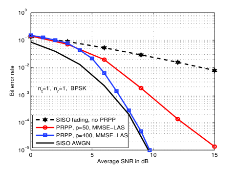
Figure 2: Performance of PRPP in SISO fading with $p=50,400$, BPSK, and LAS detection.

II-B SM system

The SM system uses $n_{t}$ transmit antennas but only one transmit RF chain as shown in Fig. 3. The number of transmit RF chains, $n_{rf}=1$. In a given channel use, the transmitter selects one of its $n_{t}$ transmit antennas, and transmits a modulation symbol from the alphabet ${\mathbb{A}}$ on the selected antenna. The number of bits transmitted per channel use through the modulation symbol is $\lfloor\log_{2}|{\mathbb{A}}|\rfloor$, and the number of bits conveyed per channel use through the index of the transmitting antenna is $\lfloor\log_{2}n_{t}\rfloor$. Therefore, a total of $\lfloor\log_{2}|{\mathbb{A}}|\rfloor+\lfloor\log_{2}n_{t}\rfloor$ bits per channel use (bpcu) is conveyed. For example, in a system with $n_{t}=2$, 8-QAM, the system throughput is 4 bpcu.

Figure 3: SM transmitter with $n_{t}$ antennas and one transmit RF chain.

Figure 4: Proposed PRPP-SM system.

The SM alphabet set for a fixed $n_{t}$ and ${\mathbb{A}}$ is given by

$${\mathbb{S}}_{n_{t},{\mathbb{A}}}=\big{\{}{\bf x}_{j,l}:j=1,\cdots,n_{t},\ \ l=1,\cdots,|{\mathbb{A}}|\big{\}},$$

$$\mbox{s.t.}\ \ {\bf x}_{j,l}=[0,\cdots,0,\underbrace{s_{l}}_{{\scriptsize{\mbox{$j$th coordinate}}}},0,\cdots,0]^{T},\ \ x_{l}\in\mathbb{A}.$$ (2)

For example, for $n_{t}=2$ and 4-QAM, ${\mathbb{S}}_{n_{t},{\mathbb{A}}}$ is given by

$${\mathbb{S}}_{2,\mbox{{\tiny 4-QAM}}} = \Bigg{\{}\begin{bmatrix}+1+j\\ 0\end{bmatrix},\begin{bmatrix}+1-j\\ 0\end{bmatrix},\begin{bmatrix}-1+j\\ 0\end{bmatrix},\begin{bmatrix}-1-j\\ 0\end{bmatrix},$$ (3)

$$\begin{bmatrix}0\\ +1+j\end{bmatrix},\begin{bmatrix}0\\ +1-j\end{bmatrix},\begin{bmatrix}0\\ -1+j\end{bmatrix},\begin{bmatrix}0\\ -1-j\end{bmatrix}\Bigg{\}}.$$

Let ${\bf x}\in{\mathbb{S}}_{n_{t},{\mathbb{A}}}$ denote the transmit vector. Let ${\bf H}\in\mathbb{C}^{n_{r}\times n_{t}}$ denote the channel gain matrix, where $H_{i,j}$ denotes the channel gain from the $j$th transmit antenna to the $i$th receive antenna, assumed to be i.i.d complex Gaussian with zero mean and unit variance. The received signal at the $i$th receive antenna is

$$y_{i}=H_{i,j}x_{l}+n_{i},\quad\quad i=1,\cdots,n_{r},$$ (4)

where $n_{r}$ is the number of receive antennas, $x_{l}$ is the $l$th symbol in ${\mathbb{A}}$ transmitted by the $j$th antenna, and $n_{i}$ is the noise component. The signals received at all the receive antennas can be written in vector form as

$${\bf y} = {\bf H}{\bf x}+{\bf n},$$ (5)

For this system model, the ML detection rule is given by

$$\hat{{\bf x}}=\mathop{\text{argmin}}_{{\bf x}\in{\mathbb{S}}_{n_{t},{\mathbb{A}}}}\ \|{\bf y}-{\bf H}{\bf x}\|^{2}.$$ (6)

III Proposed PRPP-SM system

The proposed PRPP-SM transmitter consists of $n_{t}$ transmit antennas and $n_{rf}=1$ transmit RF chains as shown in Fig. 4. It takes $p$ modulated symbols and forms the symbol vector ${\bf x}_{s}\in{\mathbb{A}}^{p}$, where ${\mathbb{A}}$ is the modulation alphabet. Let the matrix ${\bf A}$ of size $pn_{t}\times p$ denote the transmit antenna activation pattern, such that ${\bf A}{\bf x}_{s}\in{\mathbb{S}}_{n_{t},{\mathbb{A}}}^{p}$, where ${\mathbb{S}}_{n_{t},{\mathbb{A}}}$ is the SM signal set given by (2). The matrix ${\bf A}$ consists of $p$ submatrices ${\bf A}_{(i)}$, $i=1,\cdots,p$, each of size $n_{t}\times p$, such that ${\bf A}=[{\bf A}_{(1)}^{T}\,{\bf A}_{(2)}^{T}\,\cdots\,{\bf A}_{(p)}^{T}]^{T}$. The submatrix ${\bf A}_{(i)}$ is constructed as

$${\bf A}_{(i)}=[{\bf 0}_{(1)}\,\cdots\,{\bf 0}_{(i-1)}\,{\bf a}_{(i)}\,{\bf 0}_{(i+1)}\,\cdots\,{\bf 0}_{(p)}],$$ (7)

where ${\bf 0}_{(k)}$ is a $n_{t}\times 1$ vector of zeroes, and ${\bf a}_{(i)}$ is a $n_{t}\times 1$ vector constructed as

$${\bf a}_{(i)}=[0\,\cdots\,0\,\underbrace{1}_{\mbox{\tiny{$j_{i}$th coordinate}}}0\,\cdots\,0]^{T},$$ (8)

where $j_{i}$ is the index of the active antenna during the $i$th channel use. Note that, with the above definitions, ${\bf A}_{(i)}{\bf x}_{s}\in{\mathbb{S}}_{n_{t},{\mathbb{A}}}$. For example, in a system with $n_{t}=2$ and $p=3$, to activate antennas 1, 2 and 1 in three consecutive channel uses, respectively, the matrix ${\bf A}$ is given by

$${{{\bf A}\ =\ \begin{bmatrix}{\bf A}_{(1)}\\ {\bf A}_{(2)}\\ {\bf A}_{(3)}\end{bmatrix}=\begin{bmatrix}1&0&0\\ 0&0&0\\ \cr\hfil\hfil\textstyle\hfil\hfil\textstyle\vrule width=2.0pt,height=0.4pt\hfil\hfil\textstyle\hskip 2.0pt\xleaders\hbox{\hskip 2.0pt\vrule width=4.0pt,height=0.4pt\hskip 2.0pt}\hskip 0.0pt plus 1.0fil minus 1.0fil\hfil\hfil\textstyle\hskip 2.0pt\vrule width=2.0pt,height=0.4pt\hfil\hfil\textstyle\cr\cr\cr}0&0&0\\ 0&1&0\\ \cr\hfil\hfil\textstyle\hfil\hfil\textstyle\vrule width=2.0pt,height=0.4pt\hfil\hfil\textstyle\hskip 2.0pt\xleaders\hbox{\hskip 2.0pt\vrule width=4.0pt,height=0.4pt\hskip 2.0pt}\hskip 0.0pt plus 1.0fil minus 1.0fil\hfil\hfil\textstyle\hskip 2.0pt\vrule width=2.0pt,height=0.4pt\hfil\hfil\textstyle\cr\cr\cr}0&0&1\\ 0&0&0\end{bmatrix}.$$ (9)

Note that the indices of the non-zero rows in matrix ${\bf A}$ gives the support of the spatially modulated vector ${\bf A}{\bf x}_{s}\in{\mathbb{S}}_{n_{t},{\mathbb{A}}}^{p}$. For example, in (9), the support given by ${\bf A}$ is $\{1,4,5\}$.

The ${\bf A}{\bf x}_{s}$ vector is then precoded as ${\bf P}{\bf A}{\bf x}_{s}$, using a rectangular precoder matrix ${\bf P}$ of size $p\times pn_{t}$. The $(r,c)$th entry of the ${\bf P}$ matrix is $\frac{1}{\sqrt{p}}e^{j\theta_{r,c}}$, where the phases $\{\theta_{r,c}\}$ are generated using a pseudo-random sequence generator, whose seed is pre-shared among the transmitter and receiver. The output of the precoder is transmitted on the selected antenna in each channel use.

Let $n_{r}$ denote the number of receive antennas. The $pn_{r}\times 1$ received signal vector at the receiver is given by

$${\bf y} = {\bf D}{\bf A}{\bf P}{\bf A}{\bf x}_{s}+{\bf n},$$ (10)

where ${\bf D}=\mbox{diag}\{{\bf H}_{(1)}\,{\bf H}_{(2)}\,\cdots\,{\bf H}_{(p)}\}$, ${\bf H}_{(i)}$ is the $n_{r}\times n_{t}$ channel matrix of the $i$th channel use, the elements of ${\bf H}_{(i)}$ are i.i.d. complex Gaussian with zero mean and unit variance, ${\bf n}$ is the $pn_{r}\times 1$ noise vector $[{\bf n}_{(1)}^{T}\,{\bf n}_{(2)}^{T}\,\cdots\,{\bf n}_{(p)}^{T}]^{T}$ where the entries of ${\bf n}_{(i)}$ are distributed as $\mathbb{C}{\cal N}(0,\sigma^{2})$. Note that $\lVert{\bf D}{\bf A}{\bf P}{\bf A}\rVert_{F}=\lVert{\bf D}{\bf A}\rVert_{F}$. This creates a $pn_{r}\times p$ virtual MIMO system. For this system model, the ML detection rule is given by

$$\{\hat{{\bf x}}_{s},\hat{{\bf A}}\}=\mathop{\text{argmin}}_{{\bf x}_{s}\in{\mathbb{A}}^{p},\forall{\bf A}}\ \|{\bf y}_{p}-{\bf D}{\bf A}{\bf P}{\bf A}{\bf x}_{s}\|^{2}.$$ (11)

The indices of the non-zero rows in $\hat{\mathbf{A}}$ and the entries of $\hat{\mathbf{x}}_{s}$ are demapped to obtain the information bits.

Note that the ML solution in (11) can be computed only for small precoder sizes because of its exponential complexity in $p$, i.e., $O((|{\mathbb{A}}|n_{t})^{p})$). In Section IV, we will establish the superiority of the PRPP-SM over conventional PRPP and SM systems using ML detection. For large precoder sizes, we propose a low complexity detection algorithm in the following subsection.

III-A Proposed PRPP-SM detector

In this subsection, we propose a local search based detection (LSD) algorithm that achieves near-ML performance in PRPP-SM systems with large $p$ at a low computational complexity. The local search detector obtains a local minima in terms of the ML cost in a local neighborhood. In the proposed PRPP-SM system, a key requirement for local search is a suitable neighborhood definition that takes into account the antenna index bits also. We propose the following neighborhood definition for the local search. The set of neighbors of a given pair of $\{{\bf A},{\bf x}_{s}\}$, denoted by ${\mathcal{N}}({\bf A},{\bf x}_{s})$, is defined as the set of all pairs $\{{\bf A}^{\prime},{\bf x}_{s}^{\prime}\}$ that satisfies one of the following three conditions:

1. ${\bf x}_{s}={\bf x}_{s}^{\prime}$ and ${\bf A}_{(i)}\neq{\bf A}_{(i)}^{\prime}$ for exactly a single index $i$.

2. ${\bf A}={\bf A}^{\prime}$ and ${\bf x}_{s}$ differs from ${\bf x}_{s}^{\prime}$ in exactly one entry.

3. ${\bf A}_{(i)}\neq{\bf A}_{(i)}^{\prime}$ for exactly a single index $i$, and for that index $i$, $x_{s}(i)\neq x^{\prime}_{s}(i)$.

For a PRPP-SM system with $n_{t}=2$, $p=2$, and ${\mathbb{A}}=\{\pm 1\}$, an example of a neighborhood is

${{{{{{{{\scriptsize\hskip 2.84526pt{\cal N}\left(\begin{bmatrix}1&0\\ 0&0\\ \cr\hfil\hfil\textstyle\hfil\hfil\textstyle\vrule width=2.0pt,height=0.4pt\hfil\hfil\textstyle\hskip 2.0pt\xleaders\hbox{\hskip 2.0pt\vrule width=4.0pt,height=0.4pt\hskip 2.0pt}\hskip 0.0pt plus 1.0fil minus 1.0fil\hfil\hfil\textstyle\hskip 2.0pt\vrule width=2.0pt,height=0.4pt\hfil\hfil\textstyle\cr\cr\cr}0&0\\ 0&1\end{bmatrix},\begin{bmatrix}+1\\ -1\end{bmatrix}\right)=\left\{\begin{matrix}\vspace{2mm}\left\{\begin{bmatrix}1&0\\ 0&0\\ \cr\hfil\hfil\textstyle\hfil\hfil\textstyle\vrule width=2.0pt,height=0.4pt\hfil\hfil\textstyle\hskip 2.0pt\xleaders\hbox{\hskip 2.0pt\vrule width=4.0pt,height=0.4pt\hskip 2.0pt}\hskip 0.0pt plus 1.0fil minus 1.0fil\hfil\hfil\textstyle\hskip 2.0pt\vrule width=2.0pt,height=0.4pt\hfil\hfil\textstyle\cr\cr\cr}0&1\\ 0&0\end{bmatrix},\begin{bmatrix}+1\\ -1\end{bmatrix}\right\},\left\{\begin{bmatrix}1&0\\ 0&0\\ \cr\hfil\hfil\textstyle\hfil\hfil\textstyle\vrule width=2.0pt,height=0.4pt\hfil\hfil\textstyle\hskip 2.0pt\xleaders\hbox{\hskip 2.0pt\vrule width=4.0pt,height=0.4pt\hskip 2.0pt}\hskip 0.0pt plus 1.0fil minus 1.0fil\hfil\hfil\textstyle\hskip 2.0pt\vrule width=2.0pt,height=0.4pt\hfil\hfil\textstyle\cr\cr\cr}0&1\\ 0&0\end{bmatrix},\begin{bmatrix}+1\\ +1\end{bmatrix}\right\},\\ \vspace{2mm}\left\{\begin{bmatrix}1&0\\ 0&0\\ \cr\hfil\hfil\textstyle\hfil\hfil\textstyle\vrule width=2.0pt,height=0.4pt\hfil\hfil\textstyle\hskip 2.0pt\xleaders\hbox{\hskip 2.0pt\vrule width=4.0pt,height=0.4pt\hskip 2.0pt}\hskip 0.0pt plus 1.0fil minus 1.0fil\hfil\hfil\textstyle\hskip 2.0pt\vrule width=2.0pt,height=0.4pt\hfil\hfil\textstyle\cr\cr\cr}0&0\\ 0&1\end{bmatrix},\begin{bmatrix}-1\\ -1\end{bmatrix}\right\},\left\{\begin{bmatrix}1&0\\ 0&0\\ \cr\hfil\hfil\textstyle\hfil\hfil\textstyle\vrule width=2.0pt,height=0.4pt\hfil\hfil\textstyle\hskip 2.0pt\xleaders\hbox{\hskip 2.0pt\vrule width=4.0pt,height=0.4pt\hskip 2.0pt}\hskip 0.0pt plus 1.0fil minus 1.0fil\hfil\hfil\textstyle\hskip 2.0pt\vrule width=2.0pt,height=0.4pt\hfil\hfil\textstyle\cr\cr\cr}0&0\\ 0&1\end{bmatrix},\begin{bmatrix}+1\\ +1\end{bmatrix}\right\},\\ \left\{\begin{bmatrix}0&0\\ 1&0\\ \cr\hfil\hfil\textstyle\hfil\hfil\textstyle\vrule width=2.0pt,height=0.4pt\hfil\hfil\textstyle\hskip 2.0pt\xleaders\hbox{\hskip 2.0pt\vrule width=4.0pt,height=0.4pt\hskip 2.0pt}\hskip 0.0pt plus 1.0fil minus 1.0fil\hfil\hfil\textstyle\hskip 2.0pt\vrule width=2.0pt,height=0.4pt\hfil\hfil\textstyle\cr\cr\cr}0&0\\ 0&1\end{bmatrix},\begin{bmatrix}+1\\ -1\end{bmatrix}\right\},\left\{\begin{bmatrix}0&0\\ 1&0\\ \cr\hfil\hfil\textstyle\hfil\hfil\textstyle\vrule width=2.0pt,height=0.4pt\hfil\hfil\textstyle\hskip 2.0pt\xleaders\hbox{\hskip 2.0pt\vrule width=4.0pt,height=0.4pt\hskip 2.0pt}\hskip 0.0pt plus 1.0fil minus 1.0fil\hfil\hfil\textstyle\hskip 2.0pt\vrule width=2.0pt,height=0.4pt\hfil\hfil\textstyle\cr\cr\cr}0&0\\ 0&1\end{bmatrix},\begin{bmatrix}-1\\ -1\end{bmatrix}\right\}\end{matrix}\right\}.}$

The proposed LSD algorithm starts with an initial solution $\{{\bf A}^{(0)},{\bf x}_{s}^{(0)}\}$, which is also the current solution. Using the defined neighborhood, the algorithm considers all the neighbors of $\{{\bf A}^{(0)},{\bf x}_{s}^{(0)}\}$ and searches for the neighbor with the least ML cost which also has a lower ML cost than the current solution. If such a neighbor is found, then this neighbor is designated as the current solution. This marks the completion of one iteration of the algorithms. The iterations are repeated until a local minima is reached (i.e., there is no neighbor better than the current solution). The solution corresponding to the local minima is declared as the final output $\{\hat{{\bf A}},\hat{{\bf x}}_{s}\}$. This algorithm is listed in Algorithm 1 below.

Algorithm 1 Listing of the proposed LSD algorithm

1:  $\mathbf{Input:y,D}$, $\mathbf{P}$

2:  Initial solution : $\{{\bf A}^{(0)},{\bf x}_{s}^{(0)}\}$, $\{\hat{{\bf A}},\hat{{\bf x}}_{s}\}=\{{\bf A}^{(0)},{\bf x}_{s}^{(0)}\}$

3:  Compute ${\cal N}(\hat{{\bf A}},\hat{{\bf x}}_{s})$

4:  $\{{\bf A}^{c},{\bf x}_{s}^{c}\}$ = $\mathop{\text{argmin}}\limits_{\{{\bf B},{\bf z}\}\in{\cal N}(\hat{{\bf A}},\hat{{\bf x}}_{s})}\,\|{\bf y}-{\bf D}{\bf B}{\bf P}{\bf B}{\bf z}\|^{2}$

5:  if  $\|{\bf y}-{\bf D}{\bf A}^{c}{\bf P}{\bf A}^{c}{\bf x}_{s}^{c}\|^{2}<\|{\bf y}-{\bf D}\hat{{\bf A}}{\bf P}\hat{{\bf A}}\hat{{\bf x}}_{s}\|^{2}$ then

6:     $\{\hat{{\bf A}},\hat{{\bf x}}_{s}\}=\{{\bf A}^{c},{\bf x}_{s}^{c}\}$

7:     Go to step 3

8:  end if

9:  $\mathbf{Output}$ : $\{\mathbf{\hat{A}},\mathbf{\hat{s}}\}$

Computing the initial support and initial solution $\{{\bf A}^{(0)},{\bf x}_{s}^{(0)}\}$: The algorithm needs the initial support matrix ${\bf A}^{(0)}$ and the initial solution vector ${\bf x}_{s}^{(0)}$. The initial support matrix is obtained as follows. Obtain a $pn_{t}\times 1$ vector ${\bf v}$ through an MMSE estimator as

$${\bf v}=({\bf D}^{H}{\bf D}+\sigma^{2}{\bf I})^{-1}{\bf D}^{H}{\bf y}.$$

The vector ${\bf v}$ consists of $p$ subvectors ${\bf v}_{(i)}$, $i=1,\cdots,p$, each of size $n_{t}\times 1$, such that ${\bf v}=[{\bf v}_{(1)}^{T}\,{\bf v}_{(2)}^{T}\,\cdots\,{\bf v}_{(p)}^{T}]^{T}$. The indices of the elements with the largest magnitude in each ${\bf v}_{(i)}$ are taken as the indices of the non-zero rows of ${\bf A}^{(0)}$. The initial solution vector is obtained through an MMSE estimator as

$${\bf x}_{s}^{(0)}={\cal Q}\left(({\bf F}^{H}{\bf F}+\sigma^{2}{\bf I})^{-1}{\bf F}^{H}{\bf y}\right),$$

where ${\bf F}={\bf D}{\bf A}^{(0)}{\bf P}{\bf A}^{(0)}$ and ${\cal Q}(.)$ denotes the Euclidean distance quantizer such that ${\bf x}_{s}^{(0)}\in{\mathbb{A}}^{p}$.

IV Simulation results

In this section, we present the simulation results on the BER performance of the proposed PRPP-SM system with ML detection (for small $p$) and LSD detection (for large $p$).

Figure 5 compares the BER performance of PRPP-SM against the performance of SM without PRPP at a spectral efficiency of 3 bpcu using ML detection. BER plots for $n_{t}=4,n_{rf}=1,n_{r}=1$, and BPSK modulation for different precoder sizes $p=2,4,5$ are shown. It is observed that that the performance of PRPP-SM is better than SM without PRPP by about 9 dB at $p=5$ and $10^{-2}$ BER. This performance advantage in favor of the PRPP-SM system is due to the diversity gain offered by the pseudo-random phase precoding.

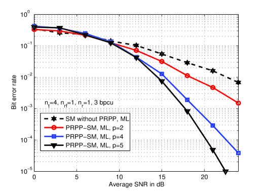
Figure 5: Performance comparison between PRPP-SM system ($n_{t}=4,n_{rf}=1,n_{r}=1$, BPSK) with ML detection and SM system without PRPP with ML detection. System throughput is 3 bpcu.

Figure 6 compares the performance of PRPP-SM against the performance of PRPP without SM (i.e., $n_{t}=1$, $p>1$) at a spectral efficiency of 3 bpcu using ML detection. Here, the PRPP-SM system has $n_{t}=4,n_{rf}=1,n_{r}=1$, BPSK modulation, and the PRPP system without SM has $n_{t}=1,n_{r}=1$, 8-QAM with varying precoder sizes $p=2,4,5$. It is observed that the performance of PRPP-SM is better than the PRPP system without SM by about 4 dB at $p=5$ and $10^{-2}$ BER. This performance advantage in favor of PRPP-SM system is mainly due to the SNR gain in using BPSK in PRPP-SM against using 8-QAM in PRPP with out SM, for the same spectral efficiency of 3 bpcu.

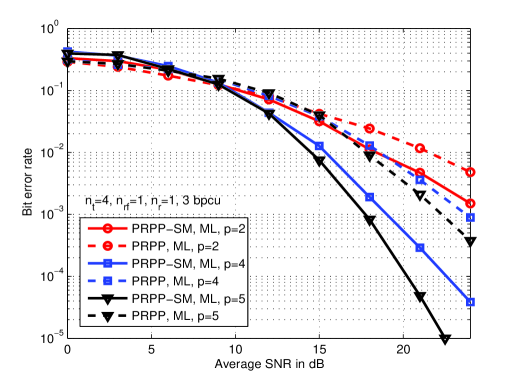
Figure 6: Performance comparison between PRPP-SM system ($n_{t}=4,n_{rf}=1,n_{r}=1$, BPSK) with ML detection and PRPP system without SM ($n_{t}=1,n_{rf}=1,n_{r}=1$, 8-QAM) with ML detection. System throughput is 3 bpcu.

Figure 7 compares the performance of PRPP-SM using the proposed LSD algorithm against the performance of PRPP without SM using LAS detection from [4]. MMSE initial solution is used in both LSD and LAS algorithms. For PRPP-SM, we have used $n_{t}=4,n_{rf}=1,n_{r}=8$, BPSK modulation. For PRPP without SM, we have used $n_{t}=1,n_{r}=8,$ 8-QAM. Large precoder sizes are used here; the precoder sizes used in both the systems are $p=10,20,70$. The spectral efficiency in both the systems is 3 bpcu. It is observed that the performance of PRPP-SM system is better than the PRPP system without SM by about 10 dB at $p$=70 and $10^{-2}$ BER. This indicates the potential of PRPP-SM system to perform very well when large precoder sizes are employed.

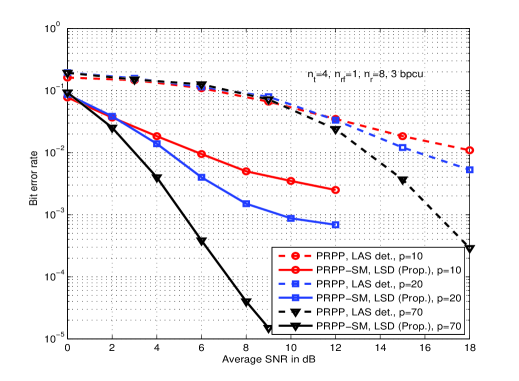
Figure 7: Comparison of the BER performance of PRPP-SM ($n_{t}=4,n_{rf}=1,n_{r}=8$, BPSK) using the proposed LSD algorithm with that of PRPP without SM ($n_{t}=n_{rf}=1,n_{r}=8$, 8-QAM) with LAS detection. System throughput is 3 bpcu.

V Conclusions

We proposed a novel pseudo-random phase precoder based spatial modulation (PRPP-SM) scheme for uncoded transmissions over fading channels. In the proposed scheme, we precoded both the modulation bits as well as the antenna index bits using a rectangular precoder matrix. Our simulation results showed that the proposed PRPP-SM system achieved diversity gains and SNR gains compared to conventional PRPP and SM systems. To facilitate the detection when large precoder sizes are used in the proposed PRPP-SM systems, we proposed a low complexity local search algorithm which used a neighborhood definition suited for taking into account the antenna index bits as well. We note that the spatial dimension in large antenna arrays can be exploited by transmitting the $p$-length precoded vector through $p$ antenna elements. This would lead to a trade-off between the number of transmit RF chains and number of channel uses. Such a generalized PRPP-SM scheme is an interesting topic for further study.

References

- [1] D. Tse and P. Viswanath, Fundamentals of Wireless Communication, Cambridge University Press, 2005.
- [2] V. Sharma, K. Premkumar and R. N. Swamy, “Exponential diversity achieving spatio-temporal power allocation scheme for fading channels,” IEEE Trans. Info. Theory, vol. 54, no. 1, pp. 188-208, Jan. 2008.
- [3] R. Annavajjala and P. V. Orlik, “Achieving near exponential diversity on uncoded low-dimensional MIMO, multi-user and multi-carrier systems without transmitter CSI,” Proc. ITA 2011, Jan. 2011.
- [4] K. V. Vardhan, S. K. Mohammed, A. Chockalingam, and B. S. Rajan, “A low-complexity detector for large MIMO systems and multicarrier CDMA systems,” IEEE J. Sel. Areas Commun., vol. 26, no. 3, pp. 473-485, Apr. 2008.
- [5] R. Mesleh, H. Hass, S. Sinaovic, C. W. Ahn, “Spatial modulation,” IEEE Trans. Veh. Tech., vol. 57, no. 4, pp. 2228-2241, Jul. 2008.
- [6] M. Di Renzo, H. Haas, A. Ghrayeb, S. Sugiura, and L. Hanzo, “Spatial modulation for generalized MIMO: challenges, opportunities and implementation,” Proceedings of the IEEE, vol. 102, no. 1, pp. 53-55, Jan. 2014.
- [7] N. Serafimovski1, S. Sinanovic, M. Di Renzo, and H. Haas, “Multiple access spatial modulation,” EURASIP J. Wireless Commun. and Networking 2012, 2012:299.
- [8] P. Raviteja, T. Lakshmi Narasimhan, and A. Chockalingam, “Multiuser SM-MIMO versus massive MIMO: uplink performance comparison,” available online: arXiv:1311.1291 [cs.IT] 6 Nov 2013.