Solutions to the quantum Rabi model with two equivalent qubits

Abstract

Using extended coherent states, an analytically exact study has been carried out for the quantum Rabi model with two equivalent qubits. Compact transcendental functions of one variable have been derived leading to exact solutions. The energy spectrum is clearly identified and analyzed. Also obtained analytically is the necessary and sufficient conditions for the occurrence of isolated exceptional solutions, which are not doubly degenerate as in the one-qubit quantum Rabi model.

1 Introduction

Quantum Rabi model (QRM) describes a two-level atom (qubit) coupled to a cavity electromagnetic mode (an oscillator)[1], a minimalist paradigm of matter-light interactions with applications in numerous fields ranging from quantum optics, quantum information science to condensed matter physics. The solutions to the QRM are however highly nontrivial. Recently, Braak presented an analytically exact solution [2] to a one-photon QRM using the representation of bosonic creation and annihilation operators in the Bargmann space of analytical functions [3]. A so-called G function with a single energy variable was derived yielding exact eigensolutions. Alternatively, using the method of extended coherent states (ECS), this G function was recovered in a simpler, yet physically more transparent manner by Chen et al.[4].

The extension of QRM to multiple qubits coupled with a single cavity mode, also known as the Dicke model[5], has also attracted considerable attention both theoretically [6, 7, 8, 9, 10, 11] and experimentally [12, 13, 14, 15, 16, 17] in the past decade. As quantum information resources such as the quantum entanglement [18] and the quantum discord [19] can be easily stored in two qubits and the Greenberger-Horne-Zeilinger (GHZ) states [20] which are generated in three qubits, it is not suprising that devices with more than one qubit find potential applications in quantum information technology[21]. More recently, some exact analytical solutions are attempted for a small number of qubits, such as two qubits[22, 23, 24] and three equivalent qubits[25] in the representation of the Bargmann space. In those studies, the G functions are often determined by matrices of high dimensions, and are therefore more complicated in form than that in the one-qubit QRM [2]. It is also a tedious task to get eigensolutions by solving coupled, highly nonlinear equations of multiple variables[22, 23, 24, 26]. In the absence of a simple G function, it is difficult to arrive at a concise description of the spectrum, and all but impossible to derive analytically a condition for the occurrence of exceptional solutions[26], which exist at special values of model parameters, and are the eigenvalues that do not correspond to zeros of the G function.

In this work, employing ECS, we demonstrate a successful derivation of a concise G function for the QRM with two equivalent qubits, similar to the case of the one-qubit QRM [2, 4]. Moreover, some isolated exact solution and the necessary and sufficient condition for its occurrence, similar to the Juddian solutions [27], are also presented.

The remainder of the paper is organized as follows. In Sec. II, a single variable G function is derived in detail for the QRM with two equivalent qubits. The solutions of these G functions and discussions about the exceptional solutions are presented in Sec. III, a brief summary is given finally.

2 The G-function

The Hamiltonian of the QRM with two equivalent qubits, also known as the Dicke model of $N=2$, can be written as

$$H={\omega}d^{{\dagger}}d+\Delta J_{z}+\frac{2\lambda}{\sqrt{N}}(d^{{\dagger}}+d)J_{x},$$ (1)

where $\Delta$ is the energy splitting of the two-level system (qubit), $d^{{\dagger}}$ creates one photon in the common single-mode cavity with frequency $\omega$, $\lambda$ describes the atom-cavity coupling strength, and

$$J_{z}=\frac{1}{2}\sum_{i=1,2}\sigma_{z}^{(i)},J_{x}=\frac{1}{2}\sum_{i=1,2}\sigma_{x}^{(i)}=\frac{1}{2}\left(J_{+}+J_{-}\right),$$ (2)

where   $\sigma_{x,z}^{(i)}~{}(i=1,2)$ is the Pauli operator of the $i-$th qubit, $J$ is the usual angular momentum operator, and $J_{+}$ and $J_{-}$ are the angular rising and lowering operators and obey the $SU(2)$ Lie algebra $[J_{+},J_{-}]=2J_{z},[J_{z},J_{\pm}]=\pm J_{\pm}$. So the Hilbert space of this algebra in this model is spanned by the Dicke state $\left|j,m_{z}\right\rangle$ with $j=1,m_{z}=-1,0,1$ and $j=0,m_{z}=0$.

There is a trivial exact eigensolution in the subspace of the $j=0$ Dicke state, because $\left|j=0,m_{z}=0\right\rangle$ is simultaneously the eigenstate of $J_{z}\$and $J_{x}$. The eigenfunction of the whole system in this subspace is $\left|n\right\rangle=\left|0,0\right\rangle\left|n\right\rangle_{\mathrm{ph}}$ where $\left|n\right\rangle_{\mathrm{ph}}=\frac{\left(d^{\dagger}\right)^{n}}{\sqrt{n!}}\left|0\right\rangle$ with eigenvalue $E_{n}=n\hbar\omega$. The solution in the space of the $j=1$ eigenstate is however highly nontrivial, and has been a subject of recent interest[11, 22, 24]. Our goal is to find analytically exact solutions with simplest forms.

A transformed Hamiltonian with a rotation with respect to the $y$ axis by an angle $\frac{\pi}{2}$ in the matrix form can be written as ( in units of $\hbar=\omega=1$)

$$H=\left(\begin{array}[]{ccc}d^{{\dagger}}d+g(d^{{\dagger}}+d)&-\frac{\Delta}{\sqrt{2}}&0\\ -\frac{\Delta}{\sqrt{2}}&d^{{\dagger}}d&-\frac{\Delta}{\sqrt{2}}\\ 0&-\frac{\Delta}{\sqrt{2}}&d^{{\dagger}}d-g(d^{{\dagger}}+d)\end{array}\right),$$ (3)

where $g=\frac{2\lambda}{\sqrt{2}}$.

In this paper, we analytically study the $N=2$ Dicke model with similar ansatz of the wavefunctions as in Ref. [9]. Note that the diagonal elements in the above matrix can be changed into free particle number operators by shifting the photonic operator with displacements $g,0,-g$. To employ our previous ECS approach[28, 9], we perform the following two Bogoliubov transformations with finite displacement

$$A=d+g,B=d-g.$$ (4)

In Bogoliubov operators $A$($B$), the matrix element $H_{11}$ ($H_{33}$) can be reduced to the free particle number operators $A^{\dagger}A$ ($B^{\dagger}B$) plus a constant, which is very helpful for the further study.

First, the wavefunction is proposed in terms of operator $A$ as

$$\left|{}\right\rangle=\left(\begin{array}[]{c}\sum_{n=0}^{\infty}\sqrt{n!}u_{n}|n\rangle_{A}\\ \sum_{n=0}^{\infty}\sqrt{n!}v_{n}|n\rangle_{A}\\ \sum_{n=0}^{\infty}\sqrt{n!}w_{n}|n\rangle_{A}\end{array},\right)$$ (5)

where $u_{n},v_{n},$and $f_{n}$ are the expansion coefficients, $\left|n\right\rangle_{A}\;$is just called extended coherent state with the following properties

$$\left|n\right\rangle_{A} = \frac{\left(A^{\dagger}\right)^{n}}{\sqrt{n!}}\left|0\right\rangle_{A}=\frac{\left(d^{\dagger}+g\right)^{n}}{\sqrt{n!}}\left|0\right\rangle_{A},$$ (6)

$$\left|0\right\rangle_{A} = e^{-\frac{1}{2}g^{2}-gd^{\dagger}}\left|0\right\rangle.$$ (7)

where the vacuum state $\left|0\right\rangle_{A}$ of the Bogoliubov operators $A$ is a well-defined eigenstate of the one-photon annihilation operator $d$, also known as a coherent state or a displaced oscillator [29].

The Schrödinger equation leads to

$$E\sum_{n=0}^{\infty}\sqrt{n!}u_{n}|n\rangle_{A} = \sum_{n=0}^{\infty}\sqrt{n!}[(n-g^{2})u_{n}-\frac{\Delta}{2}\sqrt{2}v_{n}]|n\rangle_{A},$$

$$E\sum_{n=0}^{\infty}\sqrt{n!}v_{n}|n\rangle_{A} = \sum_{n=0}^{\infty}\sqrt{n!}\{[(n+g^{2})v_{n}-\frac{\Delta}{2}\sqrt{2}(u_{n}+w_{n})]|n\rangle_{A}$$

$$-g(\sqrt{n+1}v_{n}|n+1\rangle_{A}+\sqrt{n}v_{n}|n-1\rangle_{A})\},$$

$$E\sum_{n=0}^{\infty}\sqrt{n!}w_{n}|n\rangle_{A} = \sum_{n=0}^{\infty}\sqrt{n!}\{[(n+3g^{2})w_{n}-\frac{\Delta}{2}\sqrt{2}v_{n}]|n\rangle_{A}$$

$$-2g(\sqrt{n+1}w_{n}|n+1\rangle_{A}+\sqrt{n}w_{n}|n-1\rangle_{A})\}.$$

Projecting the above three equations onto ${}_{A}\langle m|$ yields

$$Eu_{m} = (m-g^{2})u_{m}-\frac{\Delta}{\sqrt{2}}v_{m},$$ (8)

$$Ev_{m} = (m+g^{2})v_{m}-\frac{\Delta}{\sqrt{2}}(u_{m}+w_{m})-gv_{m-1}-g(m+1)v_{m+1},$$ (9)

$$Ew_{m} = (m+3g^{2})w_{m}-\frac{\Delta}{\sqrt{2}}v_{m}-2gw_{m-1}-2g(m+1)w_{m+1}.$$ (10)

Similarly, using the second operator $B$, the wavefunction can be expressed as

$$|\rangle=\left(\begin{array}[]{c}\sum_{n=0}^{\infty}(-1)^{n}\sqrt{n!}w_{n}^{\prime}|n\rangle_{B}\\ \sum_{n=0}^{\infty}(-1)^{n}\sqrt{n!}v_{n}^{\prime}|n\rangle_{B}\\ \sum_{n=0}^{\infty}(-1)^{n}\sqrt{n!}u_{n}^{\prime}|n\rangle_{B}\end{array}\right),$$ (11)

Proceeding as before, we have

$$Eu_{m}^{\prime} = (m-g^{2})u_{m}^{\prime}-\frac{\Delta}{\sqrt{2}}v_{m}^{\prime},$$ (12)

$$Ev_{m}^{\prime} = (m+g^{2})v_{m}^{\prime}-\frac{\Delta}{\sqrt{2}}(u_{m}^{\prime}+w_{m})^{\prime}-gv_{m-1}^{\prime}-g(m+1)v_{m+1}^{\prime},$$ (13)

$$Ew_{m}^{\prime} = (m+3g^{2})w_{m}^{\prime}-\frac{\Delta}{\sqrt{2}}v_{m}^{\prime}-2gw_{m-1}^{\prime}-2g(m+1)w_{m+1}^{\prime}.$$ (14)

From Eqs. $\left(\ref{coeff_A}\right)\$and $\left(\ref{coeff_B}\right),$ we can set $\ (u^{\prime},v^{\prime},w^{\prime})\ =r^{\prime}(u,v,w)$, because they satisfy the same equation. If both wave functions $\left(\ref{wave_A}\right)$ and $\left(\ref{wave_B}\right)$ are true eigenfunctions for a nondegenerate eigenstate with eigenvalue $E$, they should be proportional with each other, so with a complex constant $r,\$we can write

$$\sum_{m=0}^{\infty}\sqrt{m!}u_{m}|m\rangle_{A} = r\sum_{m=0}^{\infty}(-1)^{m}\sqrt{m!}w_{m}|m\rangle_{B},$$ (15)

$$\sum_{m=0}^{\infty}\sqrt{m!}v_{m}|m\rangle_{A} = r\sum_{m=0}^{\infty}(-1)^{m}\sqrt{m!}v_{m}|m\rangle_{B},$$ (16)

$$\sum_{m=0}^{\infty}\sqrt{m!}w_{m}|m\rangle_{A} = r\sum_{m=0}^{\infty}(-1)^{m}\sqrt{m!}u_{m}|m\rangle_{B}.$$ (17)

Left multiplying ${}_{A}\langle n|$ followed by the use of $\ \sqrt{n!}\left\langle 0\right||n\rangle_{A}=(-1)^{n}\sqrt{n!}\left\langle 0\right||n\rangle_{B}=e^{-g^{2}/2}g^{n}\$ yields

$$\sum_{n=0}^{\infty}u_{n}g^{n}=r\sum_{n=0}^{\infty}w_{n}g^{n},\ \sum_{n=0}^{\infty}v_{n}g^{n}=r\sum_{n=0}^{\infty}v_{n}g^{n},\ \sum_{n=0}^{\infty}w_{n}g^{n}=r\sum_{n=0}^{\infty}u_{n}g^{n}.$$ (18)

Eliminating the ratio constant $r$ gives $\ \left(\sum_{n=0}^{\infty}u_{n}g^{n}\right)^{2}=\left(\sum_{n=0}^{\infty}w_{n}g^{n}\right)^{2},\$ then we define a $G-$function as

$$G_{\pm}=\sum_{n=0}^{\infty}\left[u_{n}\mp w_{n}\right]g^{n},$$ (19)

where $-\left(+\right)\$ sign on the right hand side corresponds to even (odd) parity”.

To this end, we can not define the $G$ function by one coefficient determined through a linear three-term recurrence relation. To remedy this problem, we will borrow the help of the third representation of the wavefunction.

The wave function can be expanded in the Fock states, as in the one-qubit QRM [30] with a common feature of the conservation of parity

$$|\rangle=\left(\begin{array}[]{c}\sum_{n=0}^{\infty}\sqrt{n!}a_{n}|n\rangle\\ \sum_{n=0}^{\infty}\sqrt{n!}b_{n}|n\rangle\\ \pm\sum_{n=0}^{\infty}\sqrt{n!}\left(-1\right)^{n}a_{n}|n\rangle\end{array}\right),$$ (20)

where $+\left(-\right)$ stands for even (odd) parity. We then can get a set of equations

$$Ea_{m} = ma_{m}-\frac{\Delta}{\sqrt{2}}b_{m}+ga_{m-1}+g(m+1)a_{m+1},$$ (21)

$$Eb_{m} = mb_{m}-\frac{\Delta}{\sqrt{2}}\left[1\pm\left(-1\right)^{m}\right]a_{m},$$ (22)

which gives a linear three-term recurrence relation

$$a_{m+1}=\frac{1}{g(m+1)}\left[\left(E-m-\frac{\Delta^{2}}{2\left(E-m\right)}\left[1\pm\left(-1\right)^{m}\right]\right)a_{m}-ga_{m-1}\right].$$ (23)

Setting $a_{0}=1$, we can obtain coefficients $a_{m}\$ as a function of $E$ recursively, and $b_{m}$ are related to $a_{m}$ by

$$b_{m}=-\frac{\frac{\Delta}{\sqrt{2}}\left[1\pm\left(-1\right)^{m}\right]}{E-m}a_{m}.$$ (24)

Note that $b_{2k+1}=0$ for even parity, and $b_{2k}=0$ for odd parity.

Now, with the coefficients $a_{m}$, we can obtain all coefficients $u_{m},v_{m}$ and $w_{m}$ with only one variable $E$. If both wave functions $\left(\ref{wave_A}\right)$ and $\left(\ref{wave_d}\right)$ are true eigenfunctions for a nondegenerate eigenstate with eigenvalue $E$, they should be in principle only different by a complex constant $r^{\prime}$,

$$\sum_{n=0}^{\infty}\sqrt{n!}u_{n}|n\rangle_{A} = r^{\prime}\sum_{n=0}^{\infty}\sqrt{n!}a_{n}|n\rangle,$$ (25)

$$\sum_{n=0}^{\infty}\sqrt{n!}v_{n}|n\rangle_{A} = r^{\prime}\sum_{n=0}^{\infty}\sqrt{n!}b_{n}|n\rangle,$$ (26)

$$\sum_{n=0}^{\infty}\sqrt{n!}w_{n}|n\rangle_{A} = \pm r^{\prime}\sum_{n=0}^{\infty}\sqrt{n!}\left(-1\right)^{n}a_{n}|n\rangle.$$ (27)

Projecting onto ${}_{A}\langle 0|$ yields the $n=0$ coefficients

$$u_{0} = \sum_{n=0}^{\infty}a_{k}\ \left(-g\right)^{k},$$ (28)

$$v_{0} = \sum_{k=0}^{\infty}b_{k\ }\left(-g\right)^{k},$$ (29)

$$w_{0} = \pm\sum_{k=0}^{\infty}\left(-1\right)^{k}a_{k}\left(-g\right)^{k}$$ (30)

where use has been made of

$${}_{\ A}\langle 0|k\rangle=\sqrt{\frac{1}{k!}}e^{-g^{2}/2}\left(-g\right)^{k}.$$ (31)

Note that $r^{\prime}$ and $e^{-g^{2}/2}\$are omitted if we are only interested in the zeros of the G-function. Then for $n\geq 1$ coefficients $u_{n}(E),v_{n}(E)\$and $w_{n}(E)\$can be derived recursively

$$v_{n} = -\frac{1}{gn}\left[\left(E-g^{2}-n+1\right)v_{n-1}+\frac{\Delta}{\sqrt{2}}(u_{n-1}+w_{n-1})+gv_{n-2}\right],$$ (32)

$$w_{n} = -\frac{1}{2gn}\left[(E-3g^{2}-n+1)w_{n-1}+\frac{\Delta}{\sqrt{2}}v_{n-1}+2gw_{n-2}\right],$$ (33)

$$u_{n} = -\frac{\frac{\Delta}{\sqrt{2}}}{E-n+g^{2}}v_{n}.$$ (34)

Inserting these coefficients to Eq. (19) finally yields a very concise G function $G_{\pm}(E)$ without the use of a high dimensional matrix. For any $E$,  the coefficients $u_{n}(E),\ v_{n}(E)$, and $w_{n}(E)$ can be expressed by only $a_{k}$ which is determined in Eq. ( 23). In this sense, this $G$ function is a transcendental function well defined mathematically in a controlled way. The solutions to the model can be given based on these simple $G$ functions with only one variable.

3 Solutions and discussions

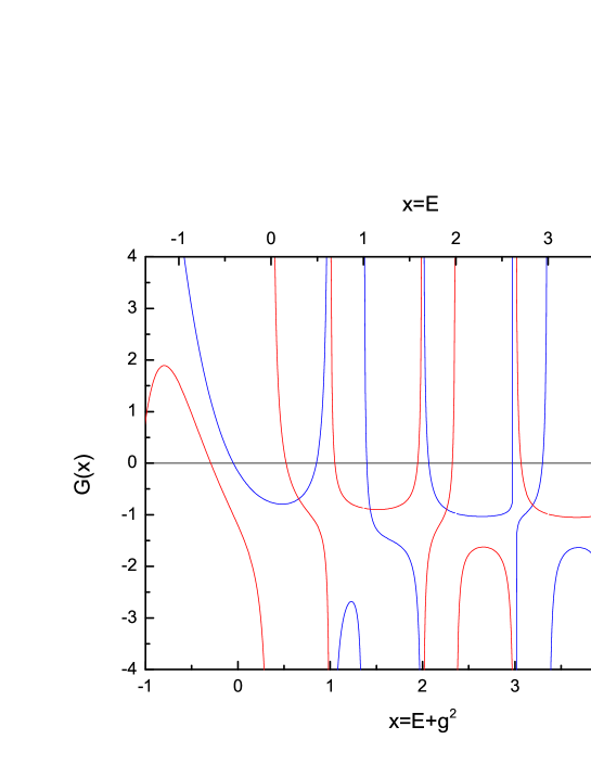
Figure 1: (Color online) G(x) curves for the two-qubit QRM at $\Delta=0.5,g=0.6$. The red (blue) one denotes even (odd) parity.

First we plot the G function in Fig. 1 for the case of $\Delta=0.5$ and $g=0.6$. As the zeros of the G function yield the eigenenergies, the exact energy levels are thus obtained as a function of the coupling constant $g$, which are then displayed in Fig. 2 for qubit splitting $\Delta=0.5$.

From Eqs. (19), (24), (29), and (34), it is obvious that the G function is not analytic at two types of poles, $E=n-g^{2}$ and $E=n$, a fact that is also clearly demonstrated in Fig. 1. The first type of poles are precisely the eigenvalues of the uncoupled bosonic mode of vanishing qubit splitting ($\Delta=0$), similar to those in one-qubit counterpart[2]. It follows that isolated exact solutions may also exist. The second type of poles are the trivial eigenvalue in the subspace $\left|j=0,m_{z}=0\right\rangle$. Such poles are, however, absent in the one-qubit QRM.

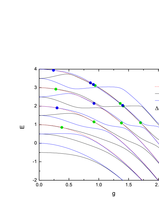
Figure 2: (Color online) The spectrum and the isolated exceptional solutions for the two-qubit QRM at $\Delta=0.5$.

In the one-qubit QRM, Koc et al. have obtained isolated exact solutions[31], which are the Juddian solutions [27] with doubly degenerate eigenvalues. These analytical solution at some isolated points can serve as benchmarks to test various approximate approaches developed for the entire parameter space. In the context of the $G$ function, these isolated eigenvalues do not correspond to the zeros of the $G$ functions, and are therefore called exceptional solutions[2]. In the two-photon QRM, these isolated exact solutions[32] are elusive in the absence of the single-variable G functions[26]. It is however easily derived later on the basis of the single variable G function[4]. In the scheme of ECS, we know that these isolated solutions with degenerate eigenstates are naturally excluded from the zeros of $G$ function on the basis of proportionality. In this work, the single variable G-function obtained for the two-qubit QRM allows an in-depth discussion of the two types of poles.

(1) Exceptional solutions at $E=m-g^{2}$. On the first type of poles at $E=m-g^{2}$, the necessary and sufficient condition for the occurrence of the exceptional eigenvalue is that the numerator ($v_{m})\$in $u_{m}$ given by Eq. (34) vanishes so that the pole at $x=m$ is lifted. Eq. (27) gives the condition for which the poles are removed:

$$\sum_{n=0}^{\infty}\sqrt{n!}\ b_{n}^{(\pm)}D_{mn}=0,$$ (35)

where

$$D_{mn}=\left(-g\right)^{n-m}\sqrt{\frac{m!}{n!}}L_{m}^{n-m}(g^{2})=\left(-1\right)^{n-m}D_{nm}.$$ (36)

Here, for $m\leq n,\ L_{m}^{n-m}(g^{2})$ is Laguerre polynomial,$\ b_{n}^{(\pm)}\$ is determined through Eqs. (23) and (24) with even and odd parity. For the same $\Delta$, the numerator $v_{m}$ is parity dependent, therefore in general, $g_{m}^{(+)}\neq g_{m}^{(-)}$, in sharp contrast with one-qubit QRM with both one photon [2] and two photons [4], where the numerator is parity independent.

Using the condition (35) of the exceptional solution, one can obtain $g_{m}^{(\pm)}$ at $E=m-g^{2}$ without the help of the $G$ function. The positions of the isolated solutions are also collected in Fig. 2. Very interestingly, they are just the crossing points of curves for $E=m-g^{2}$ and the corresponding energy levels $E^{\pm}(g)$, indicating that at least one type of exceptional solutions in this model has the form $E=m-g^{2}$.

To show the characteristics of the G function at these isolated points, in Fig. 3 we plot $G(x)$ with $E=2-g^{2}$ at given $g_{m=2}^{(\pm)}$ for the case of $\Delta=0.5$. It is clearly demonstrated that the pole at $x=2$ is removed due to the vanishing numerator, and $x=2$ is an exceptional solution because $G_{\pm}(x=2)\neq 0$. However, the poles of $G_{-}(x)$ at $g_{m=2}^{(+)}$ and of $G_{+}(x)$ at $g_{m=2}^{(-)}$ remain. These exceptional solutions are not the degenerate eigenvalues, at variance with those in the one-qubit QRM. Without degeneracy, $G_{+}(x)$ must be zero at $g_{m}^{(+)}$ if the eigenstate is given by Eq. (5). It is concluded that the wave function can not be described by an expansion of the displaced operator $A=d+g$ as in Eq. (5) at these isolated points shown as filled circles in Fig. 2.

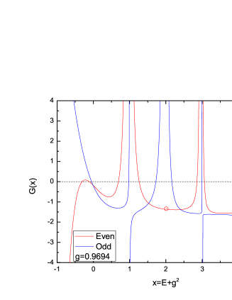
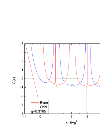
Figure 3: (Color online) G(x) at exceptional solutions for $E=2-g^{2}$. Other parameters are the same as in Fig. 2.

In the one-qubit QRM, the exceptional eigenvalues occur at some level crossing points[2, 4], the proportionality between the two wave functions in these doubly degenerate states is lacking, we may not have $G_{\pm}(x)=0$, and so the doubly degenerate eigenstate is still describable in terms of operator $A$ with displacements $\pm g$ as in Eqs. ( 5) and  (11). For the two-qubit QRM, however, this is not the case. In other words, the exact solutions exist for the one-qubit QRM, in contrast to quasi-exact solutions in the two-qubit QRM. This difference may be responsible for the integrability in one-qubit QRM and quasi-integrability in the Dicke model with $N\geq 2$.

(2) Isolated poles at $E=n$. Is there a second kind of exceptional solutions of the form $E=n$? In the recursive relation Eqs. (23) and (24), we note that the coefficient diverges for even $n$ in the even parity and odd $n$ in the odd parity, consistent with the behavior of the calculated $G$ function in Fig. 1. Can the pole at $E=n$ be removed for a certain model parameter so that the G function at this point remains analytical? It is required that numerator $a_{n}$ in Eq. (24) vanishes at $E=n$. For $n=0,$ $b_{0}=-\sqrt{2}\Delta/E$ diverges at $E=0$ for even parity, while for $n=1,$ $b_{1}=\frac{\sqrt{2}E\Delta}{g\left(E-1\right)}$ diverges at $E=1$ for odd parity. So at $E=0,1$, $G(x)$ always diverges for any model parameters, and there exists no exceptional solution. For $n=2,\ b_{n}$ diverges at $E=2$ for even parity as

$$b_{2}=-\frac{\Delta}{\sqrt{2}g^{2}}\frac{\left(E-1\right)\left(E-\frac{\Delta^{2}}{E}\right)+g^{2}}{\left(E-2\right)}.$$ (37)

Hence it is only possible for the numerator to vanish at $g_{2}=\sqrt{\frac{\Delta^{2}-4}{2}}$ for $\Delta\geq 2$. But it is found in our calculations that not even $g_{2}$ is at the crossing point of the $E=2$ line and the energy levels. Therefore, $E=n$ is only an isolated pole, not an exceptional solution, in sharp contrast to $E=n-g^{2}$. It makes sense physically. The eigenvalue $E=n$ of the spin singlet state $\left|n\right\rangle=\left|0,0\right\rangle\left|n\right\rangle_{\mathrm{ph}}$ should be independent of the nontrivial states in the $j=1$ subspace. So it is impossible that $E=n$ is an exceptional solution for the G functions derived in the $j=1$ subspace. It only points to some intrinsic relations between the two subspaces sharing the common quantum number $m_{z}=0$ in the the same system. In addition, it is our belief that these poles are not the origin of the quasi-integrability of the QRM with two qubits, because they are also well-defined eigenvalues of this model.

4 Conclusions

In this work, we have derived for the QRM with two equivalent qubits a concise single-variable G function which leads to simple, analytical solutions. Two type of poles in the G function are observed. One is the eigenvalue of the uncoupled bosonic mode, also known as the exceptional solution. Obtained analytically is the condition for the occurrence of the exceptional solution, which is parity dependent, in sharp contrast to its one-qubit counterpart, the Juddian solution to the one-qubit QRM. The other type of poles occurs at the eigenvalue of the spin singlet state, which is not an exceptional solution. This work extends the methodology of a compact G function in the one-qubit QRM to the two-qubit case, thereby allowing a conceptually clear, practically feasible treatment to energy spectra. It is our expectation that the present approach will find more applications in the future, such as in real-time dynamics.

- [1] I. I. Rabi, Phys. Rev. 49 (1936) 324; 51 (1937) 652.
- [2] D. Braak, Phys. Rev. Lett. 107(2011) 100401 .
- [3] V. Bargmann, Comm. Pure Appl. Math. 14(1961) 197.
- [4] Q. H Chen, C. Wang, S. He, T. Liu, and K. L. Wang, Phys. Rev. A 86(2012) 023822.
- [5] R. H. Dicke, Phys. Rev. 93(1954) 99.
- [6] C. Emary and T. Brandes, Phys. Rev. E 67(2003) 066203; Phys. Rev. Lett. 90(2003) 044101.
- [7] G. Liberti, F. Plastina, and F. Piperno, Phys. Rev. A 74(2006) 022324 .
- [8] J. Vidal and S. Dusuel, Europhys. Lett. 74(2006) 817.
- [9] Q. H. Chen, Y. Y. Zhang, T. Liu, and K. L. Wang, Phys. Rev. A 78(2008) 051801(R) ; T. Liu, Y. Y. Zhang, Q. H. Chen, and K. L. Wang, Phys. Rev. A 80(2009) 023810.
- [10] M. A. Bastarrachea-Magnani, J. G. Hirsch, Rev. Mex. Fis. 57, 69(2011).
- [11] S. Agarwal, S. M. Hashemi Rafsanjani, and J. H. Eberly, Phys. Rev. A 85(2012) 043815 .
- [12] M. Scheibner et al., Nature Phys. 3(2007) 106.
- [13] D. Schneble et al., Science 300(2003) 475.
- [14] M. J. Hartmann et al., Nature Phys. 2, 849(2006); A. D. Greentree et al., ibid. 2(2006) 856.
- [15] P. Nataf and C. Ciuti, Nature Comm. 1 (2010) 72; Phys. Rev. Lett. 104(2010) 023601.
- [16] A. Vukics and P. Domokos, Phys. Rev. A 86 053807(2012).
- [17] K. Baumann, C. Guerlin, F. Brennecke and T. Esslinger, Nature 464(2010) 1301.
- [18] M. A. Nielsen and I. L. Chuang, Quantum Computation and Quantum Information (Cambridge University Press, Cambridge, England, 2000).
- [19] H. Ollivier and W. H. Zurek, Phys. Rev. Lett. 88 (2001) 017901; W. H. Zurek, Phys. Rev. A 67(2003) 012320.
- [20] D. M. Greenberger, M. Horne, A. Shimony, and A. Zeilinger, Am. J. Phys. 58(1990) 1131.
- [21] M. A. Sillanpaa, J. I. Park, and R. W. Simmons R W, Nature 449(2007) 438; G. Haack, F. Helmer, M. Mariantoni,F. Marquardt and E. Solano, Phys. Rev. B 82(2010) 024514; F. Altintas and R. Eryigit, Phys. Lett. A 376(2012) 1791.
- [22] S. A. Chilingaryan and B. M. Rodriguez-Lara, J. Phys. A. : Math. Theor 46(2013) 335301.
- [23] B. M. Rodriguez-Lara, J. Phys. A: Math. Theor. 47 (2014)135306.
- [24] J. Peng et al. arXiv: 1312.7610 (2013).
- [25] D. Braak, J. Phys. B: At. Mol. Opt. Phys. vol. 46 (2013) 224007.
- [26] I. Travěnec, Phys. Rev. A 85 (2012) 043805.
- [27] B. R. Judd, J. Phys. C 12 (1979) 1685.
- [28] Q. H. Chen, Y. Yang, T. Liu, and K. L. Wang, Phys. Rev. A 82 (2010) 052306; Y. Y. Zhang, Q. H. Chen, and K. L. Wang, Phys. Rev. B 81(2010) 121105 (R).
- [29] R. J. Glauber, Phys. Rev. 131(1963) 2766 .
- [30] S. He, C. Wang, Q. H Chen, X. Z. Ren, T. Liu, and K. L. Wang, Phys. Rev. A 86(2012) 033837.
- [31] R. Koc, M. Koca, and H. H. Tütüncüler, J. Phys. A: Math. Gen. 35(2002) 9425.
- [32] C. Emary and R. F. Bishop, J. Phys. A 35(2002) 8231 .