An approach to normal forms of Kuramoto model with distributed delays and the effect of minimal delay

Abstract

Heterogeneous delays with positive lower bound (gap) are taken into consideration in Kuramoto oscillators. We first establish a perturbation technique, by which universal normal forms and detailed dynamical behavior of this model can be obtained easily. Theoretically, a hysteresis loop is found near the subcritically bifurcated coherent state on the Ott-Antonsen’s manifold. For Gamma distributed delay with fixed variance and mean, we find large gap destroys the loop and significantly increases in the number of coexisted coherent attractors. This result is also explained in the viewpoint of excess kurtosis.

I Introduction

The Kuramoto phase oscillators were used to model diverse situations involving large community of oscillators article1001 ; article1002 ; article1003 ; article1004 ; article1005 ; article1006 ; article1007 ; article1008 ; article1009 ; article1110 ; article1111 ; article1112 , where the state of every oscillator is determined by a phase on the unit circle. This model captures essential features of synchronization, observed in many physical modelsarticle1501 ; article1502 ; article1503 ; article1504 ; article1505 ranging from biology, neural science, lasers, engineering to superconducting Josephson junctions. Kuramotoarticle5 extended Winfree’s mean-field ideaarticle10 , and confirmed that one population of weakly nearly-identical coupled oscillators could be depicted as a universal model

$$\dot{\theta}_{i}=\omega_{i}+\sum\limits_{j=1}^{N}\frac{K}{N}\sin(\theta_{j}-\theta_{i}),~{}i=1,2,\ldots,N$$

Here the frequencies $\omega_{i}$ follow some distribution with probability density function (PDF) $g(\omega)$.

In a network, signal’s transmission and receive both lead to time delays. Thus considering time lag is necessary in many coupled systemsar9 ; ar92 ; ar921 . Due to the spatio-distribution of oscillators, the transmitting delays among oscillators may be heterogenous. They may follow some probability distributions such as Gamma distribution, because the lag can be viewed as a period of awaiting. In a network with near-identical oscillators, the receiving delay, or responding delay, can be viewed as a constant. Hence, the total delay usually follows certain probability distribution with a gap, i.e., the positive lower bound. Other examples with a gap usually arise in the biomathematical problems. In population dynamics, the mature delay is an important parameter which is distributed in an interval with positive lower boundgap1 . Thus in a prey-predator network, introducing heterogeneous delays with a gap should be greater realism. When dealing with different problems such as the growth of phytoplankton, the mature delay could also be replaced by time lag to digest nutrientsgap2 . Time lags with a gap have also been used extensively when modelling traffic flow dynamicsgap3 , machine tool vibration problemgap4 and so ongap5 .

Lee et alwai , using the Ott-Antonsen’s manifold reduction methodott2 , found that the variation of delay could greatly alter the dynamical behavior in a Kuramoto model with distributed delay without a gap. This paper offered a framework for studying the delay heterogeneity, where the results are illustrated with respect to Gamma-distributed time lags in $[0,+\infty)$. After some simulations, both supercritical and subcritical Hopf bifurcations on the mean-field are observed.

On one hand, in mathematical consideration, the mechanism causing the above phenomena is not quite clear yet, which depends on further bifurcation analysis. Using bifurcation technique, the transition among different schemes can be detected clearly. On the other, when time lag distributes in the interval $[\tau_{0},+\infty)$ with a minimal responding time $\tau_{0}>0$, this is the case rarely investigated before. The total delay may be the sum of a Gamma distributed delay $\tilde{\tau}\sim\Gamma(n,\frac{T}{n})$ and a constant $\tau_{0}$ (See FIG. 1(a)), for example. In this case, an interesting fact is that studying only the mean and variance of delays sometimes does not make any senses. For instance, by varying $n$, one can still fix the expectation of total delay $\langle\tau\rangle=\langle\tilde{\tau}+\tau_{0}\rangle=T+\tau_{0}$, and its variance $\textrm{Var}(\tau)=\frac{T^{2}}{n}$ despite the ratio $\frac{\tau_{0}}{T+\tau_{0}}$ varies (See FIG. 1(b)). Thus the gap $\tau_{0}$ may have certain effect on the system dynamics without changing $\langle\tau\rangle$ and $\textrm{Var}(\tau)$. In this case higher order moments of the data should be considered such as skewness or excess kurtosis, which involve the third-order or fourth-order central moments and are usually used to measure the “asymmetry” or the “peakedness” of probability distribution, respectively. So far as we know, these two points of view are new and have not been well studied.

(a)                                                           (b)
 

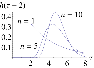
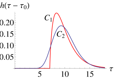
Figure 1: (a) $h(\tau-\tau_{0})$, PDFs of the sum of Gamma distribution $\tilde{\tau}\sim\Gamma(n,\frac{T}{n})$ with $T=3$, $n=1,5,10$ and $\tau_{0}=2$. (b) Two PDFs of Gamma distribution with a gap, $C_{1}$: (red) $T=3,\tau_{0}=7$ with larger excess kurtosis; $C_{2}$: (blue) $T=7,\tau_{0}=3$ with smaller excess kurtosis. $n$ is suitably chosen such that variance $T^{2}/n=5$.

Motivated by the above two considerations and these pioneer works, we are about to consider a more realistic case: heterogeneous delays with a positive minimal delay in a system, or a gapyuan , we say. Now the Kuramoto model reads

$$\dot{\theta}_{i}=\omega_{i}+\frac{k}{N}\sum_{j=1}^{N}\sin[\theta_{j}(t-\tau_{i})-\theta_{i}(t)]$$ (1)

$i=1,2,\ldots,N$, where $\theta_{i}(t)\in[0,2\pi)$ is the phase of the $i$th oscillator and $\omega_{i}$ is its natural frequency coming from an ensemble with PDF $g(\omega),\omega\in(-\infty,+\infty)$. $k$ is the constant coupling strength. The delays $\tau_{i}$, coming from the ensemble $\tau$, are statistically independent with $\omega_{i}$. In this paper, we choose random variable $\tau=\tilde{\tau}+\tau_{0}$ with $\tilde{\tau}$ having PDF $h(\tau)$ and $\tau_{0}$ a constant. Thus $\tau_{i}$ can be viewed as following a new distribution with PDF $h(\tau-\tau_{0}),\tau\in[\tau_{0},+\infty)$.

In this paper, we will give some bifurcation results about system (1). After reducing it onto the Ott-Antonsen’s manifold, a delay differential equation is obtained, in which a Hopf bifurcation at the trivial solution means the coherent state is bifurcating from the incoherent state. In our earlier workniuphyd , the center manifold reduction methodHassardfaria ; Hassardfaria is employed to investigate this bifurcation. However, the calculations depend on a rather complicated decomposition of a Banach space and many Riemann-Stieltjes integrals. Here, we make this approach much easier, and use the method of multiple scalesnams ; nams1 ; nams2 to give a relatively simple calculation process of the normal forms, by which the direction and the stability of the bifurcated coherent state are determined. For Gamma distributed delay, we calculate all bifurcation points in certain parameter spaces and discuss the effect of the gap. Finally, it is found that, when fixing $\langle\tau\rangle$ and Var$(\tau)$, larger gap (or larger excess kurtosis, equivalently) not only leads to a supercritical bifurcation hence avoids the existence of hysteresis loop, but also significantly increases in the number of coexisted coherent states.

II Reduction

As $N\rightarrow\infty$, the continuity equation of (1) is

$$\frac{\partial}{\partial t}f+\frac{\partial}{\partial\theta}(\zeta f)=0$$ (2)

with a drift term $\zeta(\theta,t)=\omega+\frac{k}{2\textrm{i}}(\textrm{e}^{-\textrm{i}\theta}r-\textrm{e}^{\textrm{i}\theta}r^{\ast})$. The complex-valued “order-parameter” $r(t)$ is defined by

$$r(t)=\langle\xi(t-\tau)\rangle=\int_{\tau_{0}}^{+\infty}\xi(t-\tau)h(\tau-\tau_{0})\textrm{d}\tau$$ (3)

with

$$\xi(t)=\int_{-\infty}^{+\infty}\int_{0}^{2\pi}f(\omega,\theta,t)\textrm{e}^{\textrm{i}\theta}\textrm{d}\theta\textrm{d}\omega$$ (4)

The distribution density $f(\omega,\theta,t)$ characterizes the state of the oscillators’ system at time $t$ in frequency $\omega$ and phase $\theta$.

Now we are about to restate some results about the Ott-Antonsen’s reduction of a system with distributed delay first derived by Lee et alwai . Rewriting system (2) as

$$\frac{\partial}{\partial t}f+\frac{\partial}{\partial\theta}\left\{\left[\omega+\frac{k}{2\textrm{i}}(\textrm{e}^{-\textrm{i}\theta}r-\textrm{e}^{\textrm{i}\theta}r^{\ast})\right]f\right\}=0$$ (5)

and restricting this partial differential equation on the Ott-Antonsen manifold

$$\left\{f:f=\frac{g(\omega)}{2\pi}\left\{1+\left[\sum_{m=1}^{\infty}\alpha^{m}(\omega,t)\textrm{e}^{\textrm{i}m\theta}+c.c.\right]\right\}\right\}$$

with c.c. the complex conjugate of the formal terms, we substitute the Fourier series of $f$ into (5). After comparing the coefficient of the same harmonic terms, a reduced equation is obtained

$$\dot{\alpha}(\omega,t)=-\textrm{i}\omega\alpha(\omega,t)+\frac{k}{2}r^{\ast}-\frac{k}{2}r\alpha^{2}(\omega,t)$$ (6)

Obviously, from (4) we have $\xi(t)=\int_{-\infty}^{+\infty}g(\omega)\alpha^{\ast}(\omega,t)\textrm{d}\omega$, then Eq.(3) yields

$$r(t)=\int_{\tau_{0}}^{+\infty}\int_{-\infty}^{+\infty}g(\omega)\alpha^{\ast}(\omega,t-\tau)\textrm{d}\omega h(\tau-\tau_{0})\textrm{d}\tau$$ (7)

For the sake of theoretical analysis, the distribution density $g(\omega)$ is usually chosen as Lorentzian distribution, that is

$$g(\omega)=\frac{\Delta}{\pi[(\omega-\omega_{0})^{2}+\Delta^{2}]},~{}-\infty<\omega<+\infty$$ (8)

Note that the Lorentzian distribution is unimodal and can be viewed as an approximation of normal distribution.

Following Ott and Antonsen’s method ott2 , substituting (8) into (7), and using residue theorem, we have

$$r(t)=\int_{\tau_{0}}^{+\infty}\alpha^{\ast}(\omega_{0}-\textrm{i}\Delta,t-\tau)h(\tau-\tau_{0})\textrm{d}\tau$$ (9)

Putting $\omega=\omega_{0}-\textrm{i}\Delta$ in Eq.(6) and noticing Eq.(9) yield

$$\begin{array}[]{l}\dot{\alpha}(t)=-(\textrm{i}\omega_{0}+\Delta)\alpha(t)+\frac{k}{2}\int_{\tau_{0}}^{+\infty}\alpha(t-\tau)h(\tau-\tau_{0})\textrm{d}\tau-\frac{k}{2}\int_{\tau_{0}}^{+\infty}\alpha^{\ast}(t-\tau)h(\tau-\tau_{0})\textrm{d}\tau\alpha^{2}(t)\end{array}$$ (10)

which is a delay differential equationHalefde , whose trivial equilibrium stands for the incoherent state. To investigate its stability, we substitute $\alpha=\alpha_{0}\textrm{e}^{\lambda t}$ into the linear part of (10) with $\alpha_{0}\neq 0$, and obtain

$$\lambda=-(\textrm{i}\omega_{0}+\Delta)+\frac{k}{2}\int_{\tau_{0}}^{+\infty}\textrm{e}^{-\lambda\tau}h(\tau-\tau_{0})\textrm{d}\tau$$ (11)

Obviously, if $\Delta>0$, $\lambda=-(\textrm{i}\omega_{0}+\Delta)$ at $k=0$, thus the incoherence is stable for sufficiently small $k$. After the occurrence of Hopf bifurcation, roots with positive real part may appear in (11), which means the incoherence looses stability. At the limit of identical oscillators $\Delta\rightarrow 0$, we know the incoherence is neutrally stable at $k=0$. Once $k$ increases, the incoherent state becomes stable (or unstable) if Re $\frac{\textrm{d}\lambda}{\textrm{d}k}|_{k=0}=\frac{1}{2}\int_{\tau_{0}}^{+\infty}\cos\omega_{0}\tau h(\tau-\tau_{0})\textrm{d}\tau<0$ (or $>0$).

Usually, if (11) has a root $\lambda=\textrm{i}\beta$, a Hopf bifurcating solution $\alpha(t)=\textrm{e}^{\textrm{i}\beta t}$ appears, which stands for a coherent state in system (1). In the rest part of this paper, the stability of this coherent state and the exact location where it appears will be investigated.

III Bifurcation analysis

In this section, we assume that $\Delta>0$, and a Hopf bifurcation occurs in Eq.(10). If Hopf bifurcation occurs at $k=\bar{k}$, two necessary conditions are required: [i] Eq.(11) has a simple root $\lambda=\textrm{i}\beta$ with $\beta\neq 0$ when $k=\bar{k}$; [ii] The so-called transversality condition holds in the sense that $\textrm{Re}\lambda^{\prime}(k)\neq 0$ at $k=\bar{k}$.

To obtain more properties near $\bar{k}$, one usually should do bifurcation analysis near this critical point, including the normal form deriving and unfolding analysisWiggins2 . In a previous workniuphyd , we have done this in case of $\tau_{0}=0$. The approach therein heavily depends on a mathematical fundation such as formal adjoint theory of functional differential equation and the decomposition of Banach space. Moreover, some calculations such as Riemann-Stieltjes integrals are tedious, and we can expect that even more calculations are needed when $\tau_{0}>0$. In this section, we are about to extend the traditional method of multiple scalesnams , a classical perturbation method, to the bifurcation analysis of the complex-valued equation (10).

III.1 Normal forms

Denoting by $k=\bar{k}+\epsilon\nu$ with $\epsilon>0$ and $\nu$ a detuning parameter which describes the nearness of $k$ to the critical value $\bar{k}$, Eq.(10) can be rewritten into

$$\begin{array}[]{ll}\dot{\alpha}(t)=&-(\textrm{i}\omega_{0}+\Delta)\alpha(t)+\frac{\bar{k}+\epsilon\nu}{2}\int_{\tau_{0}}^{+\infty}\alpha(t-\tau)h(\tau-{\tau_{0}})\textrm{d}\tau\\ &-\frac{\bar{k}+\epsilon\nu}{2}\int_{\tau_{0}}^{+\infty}\alpha^{\ast}(t-\tau)h(\tau-{\tau_{0}})\textrm{d}\tau\alpha^{2}(t)\end{array}$$ (12)

For the absence of second order term in (12), the solution to Eq.(12) can be expressed byepsilon22

$$\alpha(t;\epsilon):=\epsilon^{1/2}\alpha_{1}(T_{0},T_{1})+\epsilon^{3/2}\alpha_{2}(T_{0},T_{1})+\cdots$$

where $T_{0}=t$, $T_{1}=\epsilon t$. The two time scales can be interpreted as follows. When $\nu$ is sufficiently small, i.e., near the critical point, solutions to system (12) near the trivial equilibrium oscillate in a fast time scale $T_{0}$explain , whereas they trend towards (OR depart from) a small stable (OR unstable) periodic oscillation in a slow time scale $T_{1}$. This is shown in FIG. 2.

(a)                                                           (b)

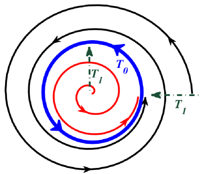
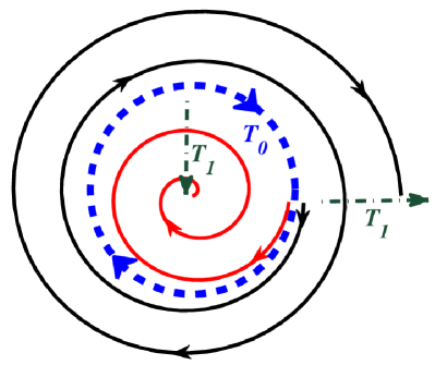
Figure 2: (a) Solutions trend towards (in scale $T_{1}$, red and black curves) a stable cycle (oscillating in scale $T_{0}$, blue). (b) Solutions depart from (in scale $T_{1}$, red and black curves) an unstable cycle (oscillating in scale $T_{0}$, blue).

The derivative with respect to $t$ is transformed into

$$\frac{\textrm{d}}{\textrm{d}t}=\frac{\partial}{\partial T_{0}}+\epsilon\frac{\partial}{\partial T_{1}}:=D_{0}+\epsilon D_{1}$$

Taylor expanding the term $\alpha(t-\tau):=\alpha(t-\tau;\epsilon)$ gives

$$\begin{array}[]{l}\alpha(t-\tau;\epsilon)=\epsilon^{1/2}\alpha_{1}(T_{0}-\tau,T_{1})+\epsilon^{3/2}\alpha_{2}(T_{0}-\tau,T_{1})-\epsilon^{3/2}\tau D_{1}\alpha_{1}(T_{0}-\tau,T_{1})+\cdots\end{array}$$

Substituting $\alpha(t)$ and $\alpha(t-\tau)$ into (12), and balancing the same order terms of $\epsilon$ in both sides we have

$$\begin{array}[]{l}D_{0}\alpha_{1}(T_{0},T_{1})=-(\textrm{i}\omega_{0}+\Delta)\alpha_{1}(T_{0},T_{1})+\frac{\bar{k}}{2}\int_{\tau_{0}}^{+\infty}\alpha_{1}(T_{0}-\tau,T_{1})h(\tau-{\tau_{0}})\textrm{d}\tau\end{array}$$ (13)

and

$$\begin{array}[]{ll}D_{0}\alpha_{2}(T_{0},T_{1})=&-(\textrm{i}\omega_{0}+\Delta)\alpha_{2}(T_{0},T_{1})+\frac{\bar{k}}{2}\int_{\tau_{0}}^{+\infty}\alpha_{2}(T_{0}-\tau,T_{1})h(\tau-{\tau_{0}})\textrm{d}\tau\\ &+\nu\frac{1}{2}\int_{\tau_{0}}^{+\infty}\alpha_{1}(T_{0}-\tau,T_{1})h(\tau-{\tau_{0}})\textrm{d}\tau-D_{1}\alpha_{1}(T_{0},T_{1})\\ &+\frac{\bar{k}}{2}\int_{\tau_{0}}^{+\infty}-\tau D_{1}\alpha_{1}(T_{0}-\tau,T_{1})h(\tau-{\tau_{0}})\textrm{d}\tau\\ &-\frac{\bar{k}}{2}\int_{\tau_{0}}^{+\infty}\alpha_{1}^{\ast}(T_{0}-\tau,T_{1})h(\tau-{\tau_{0}})\textrm{d}\tau\alpha_{1}^{2}(T_{0},T_{1})\end{array}$$ (14)

Eq.(13) is a linear equation and has a solution

$$\begin{array}[]{l}\alpha_{1}(T_{0},T_{1})=A(T_{1})\textrm{e}^{\textrm{i}\beta T_{0}}+\sum\limits_{m=1}^{+\infty}[A_{m}(T_{1})\textrm{e}^{(\sigma_{m}+\textrm{i}\beta_{m})T_{0}}]\end{array}$$

If all roots of Eq.(11) $\sigma_{m}+\textrm{i}\beta_{m},~{}m=1,2,\ldots$, except $\textrm{i}\beta$, have negative real part, $\sigma_{m}<0$ for any $m$, then $\alpha_{1}(T_{0},T_{1})\rightarrow A(T_{1})\textrm{e}^{\textrm{i}\beta T_{0}}$, as $t\rightarrow+\infty$.

Now we can find that, the bifurcated solution oscillates in time scale $T_{0}$, and all solutions nearby trend towards it in time scale $T_{1}$, if the periodic oscillation is locally attractive. Thus the dynamical behavior of $A(T_{1})$ determines the property of the bifurcation such as the stability: if a differential equation about $|A(T_{1})|$ has a stable nontrivial equilibrium, system (12) has a stable periodic solution originating from Hopf bifurcation. This is the main idea of normal form method of Hopf bifurcation [recalling FIG. 2], which will be further calculated in the following.

Substituting $\alpha_{1}(T_{0},T_{1})$ into (14) yields

$$\begin{array}[]{ll}D_{0}\alpha_{2}(T_{0},T_{1})&=-(\textrm{i}\omega_{0}+\Delta)\alpha_{2}(T_{0},T_{1})+\frac{\bar{k}}{2}\int_{\tau_{0}}^{+\infty}\alpha_{2}(T_{0}-\tau,T_{1})h(\tau-{\tau_{0}})\textrm{d}\tau\\ &+\nu\frac{1}{2}\int_{\tau_{0}}^{+\infty}A(T_{1})\textrm{e}^{\textrm{i}\beta(T_{0}-\tau)}h(\tau-{\tau_{0}})\textrm{d}\tau-A^{\prime}(T_{1})\textrm{e}^{\textrm{i}\beta T_{0}}\\ &+\frac{\bar{k}}{2}\int_{\tau_{0}}^{+\infty}-\tau A^{\prime}(T_{1})\textrm{e}^{\textrm{i}\beta(T_{0}-\tau)}h(\tau-{\tau_{0}})\textrm{d}\tau\\ &-\frac{\bar{k}}{2}\int_{\tau_{0}}^{+\infty}A^{\ast}(T_{1})\textrm{e}^{-\textrm{i}\beta(T_{0}-\tau)}h(\tau-{\tau_{0}})\textrm{d}\tau A^{2}(T_{1})\textrm{e}^{2\textrm{i}\beta T_{0}}\end{array}$$

The last four terms in the above equation lead to secular terms, because they make $\alpha_{2}(T_{0},T_{1})$ depend on $T_{0}\textrm{e}^{\textrm{i}\beta T_{0}}$, which is a contradiction. Eliminating them, we have the normal form given by

$$\begin{array}[]{ll}A^{\prime}(T_{1})&=\nu\frac{\int_{\tau_{0}}^{+\infty}\textrm{e}^{-\textrm{i}\beta\tau}h(\tau-{\tau_{0}})\textrm{d}\tau}{2+{\bar{k}}\int_{\tau_{0}}^{+\infty}\tau\textrm{e}^{-\textrm{i}\beta\tau}h(\tau-{\tau_{0}})\textrm{d}\tau}A(T_{1})+\frac{{\bar{k}}\int_{\tau_{0}}^{+\infty}\textrm{e}^{\textrm{i}\beta\tau}h(\tau-{\tau_{0}})\textrm{d}\tau}{2+{\bar{k}}\int_{\tau_{0}}^{+\infty}\tau\textrm{e}^{-\textrm{i}\beta\tau}h(\tau-{\tau_{0}})\textrm{d}\tau}A^{2}(T_{1})A^{\ast}(T_{1})\\ &:=a\nu A(T_{1})+bA^{2}(T_{1})A^{\ast}(T_{1})\end{array}$$

The amplitude equation is

$$|A(T_{1})|^{\prime}=\nu\textrm{Re}a|A(T_{1})|+\textrm{Re}b|A(T_{1})|^{3}$$

In fact, regarding $\lambda$ a function of $k$ defined implicitly by (11), we know $a=\lambda^{\prime}(\bar{k})$. According to the fundamental theory about Poincaré–Birkhoff normal form of ODEWiggins2 , the two real parts of $a$ and $b$ determine the direction and stability of the bifurcation.

Precisely, letting $k_{0}=\inf\{\bar{k}|\bar{k}$ is a Hopf bifurcation value$\}$, we always have Re$a>0$. If $\nu>0$ and Re$b<0$, then $|A(T_{1})|\rightarrow\sqrt{\frac{\nu\textrm{Re}a}{-\textrm{Re}b}}$ as $T_{1}\rightarrow\infty$. Thus a branch of stablestable bifurcation solutions appears at $k>k_{0}$ for Re$b<0$. Similarly, a branch of unstable solutions appears at $k<k_{0}$ for Re$b>0$. In the latter case, the branch of unstable solutions must go to $k>k_{0}$, because when $k=0$ system (10) has a globally stable attractor $\alpha=0$.

Two kinds of bifurcations are the so-called supercritical and subcritical bifurcations, respectively as shown in FIG. 3. If at some $\bar{k}$, Re $a<0$, there are two other kinds of bifurcations which can be illustrated by reversing the stability of coherent states.

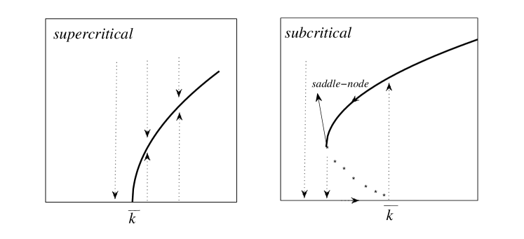
Figure 3: Supercritical bifurcation and subcritical bifurcation(with a hysteresis loop between $\bar{k}$ and the saddle-node point) near a critical value $\bar{k}$.

Consider the case time delay comes from an ensemble $\tau$ which is the sum of a Gamma distributed variable $\tilde{\tau}$ and a constant $\tau_{0}$. $\tilde{\tau}\sim\Gamma(n,\frac{T}{n})$ has PDF

$$h(\tau)=\frac{1}{\Gamma(n)(T/n)^{n}}\tau^{n-1}\textrm{e}^{-\frac{\tau}{T/n}},\tau>0$$

where $T$ is the mean value, $\frac{T^{2}}{n}$ the variance, $\frac{2}{\sqrt{n}}$ the skewness and $\frac{6}{n}$ the excess kurtosis. The PDF of $\tau$, $h(\tau-\tau_{0})$ has been shown in FIG. 1(a). The laplace transformation of $h(\tau)$ is $(1+\frac{T}{n}\lambda)^{-n}$.

The characteristic equation in this case is given by

$$\begin{array}[]{l}\lambda=-(\textrm{i}\omega_{0}+\Delta)+\frac{k}{2}\int_{\tau_{0}}^{+\infty}\textrm{e}^{-\lambda\tau}h(\tau-{\tau_{0}})\textrm{d}\tau=-(\textrm{i}\omega_{0}+\Delta)+\frac{k}{2}(1+\frac{T}{n}\lambda)^{-n}\textrm{e}^{-\lambda\tau_{0}}\end{array}$$

Motivated by the above analysis, we are seeking for a root $\lambda=\textrm{i}\beta$ and have

$$\textrm{i}\beta=-(\textrm{i}\omega_{0}+\Delta)+\frac{k}{2}(1+\frac{T}{n}\textrm{i}\beta)^{-n}\textrm{e}^{-\textrm{i}\beta\tau_{0}}$$ (15)

Denote by $1+\frac{T}{n}\textrm{i}\beta=\rho\textrm{e}^{\textrm{i}\vartheta}$, then

$$\begin{array}[]{rl}\Delta=&\frac{k}{2}\rho^{-n}\cos(n\vartheta+\beta\tau_{0})\\ \beta+\omega_{0}=&-\frac{k}{2}\rho^{-n}\sin(n\vartheta+\beta\tau_{0})\end{array}$$ (16)

Obviously, $\vartheta\in[-\pi/2,\pi/2]$, thus $\vartheta=\arctan\frac{T\beta}{n}$. Then we have

$$-\frac{\beta+\omega_{0}}{\Delta}=\tan\left[n\arctan\left(\frac{T\beta}{n}\right)+\beta\tau_{0}\right]$$

This equation can be solved by a sequence of $\beta$’s with $|\beta|\rightarrow+\infty$, for all parameters fixed. As $|\beta|\rightarrow+\infty$, we have $\rho\rightarrow\infty$, thus $k\rightarrow\infty$ holds from the first equation of (16). Hence we only need to calculate all roots for $\beta\in[-J,J]$ with $J$ relatively large, to obtain the first several bifurcation values of $\bar{k}$.

If a bifurcation occurs at $\bar{k}$, then employing the normal form theory established above, we have

$$a=\frac{(1+\frac{\textrm{i}\beta T}{n})^{-n}\textrm{e}^{-\textrm{i}\beta\tau_{0}}}{2+\bar{k}\left(\frac{T\textrm{e}^{-\textrm{i}\beta\tau_{0}}}{1+\frac{\textrm{i}\beta T}{n}}+\tau_{0}\textrm{e}^{-\textrm{i}\beta\tau_{0}}\right)\left(1+\frac{\textrm{i}\beta T}{n}\right)^{-n}}$$

$$b=-\frac{\bar{k}\textrm{e}^{\textrm{i}\beta\tau_{0}}\left(1-\frac{\textrm{i}\beta T}{n}\right)^{-n}}{2+\bar{k}\left(\frac{T\textrm{e}^{-\textrm{i}\beta\tau_{0}}}{1+\frac{\textrm{i}\beta T}{n}}+\tau_{0}\textrm{e}^{-\textrm{i}\beta\tau_{0}}\right)\left(1+\frac{\textrm{i}\beta T}{n}\right)^{-n}}$$

We claim that Re$a>0$ always holds. In fact, from (15), we have $\textrm{i}\beta+\textrm{i}\omega_{0}+\Delta=\frac{k}{2}(1+\frac{T}{n}\textrm{i}\beta)^{-n}\textrm{e}^{-\textrm{i}\beta\tau_{0}}$, then

$$\begin{array}[]{ll}&\textrm{Sign~{}Re~{}}a\\ &=\textrm{Sign~{}Re~{}}a^{-1}\\ &=\textrm{Sign~{}Re~{}}\frac{1+\left(\frac{T}{1+\frac{\textrm{i}\beta T}{n}}+\tau_{0}\right)(\textrm{i}\beta+\textrm{i}\omega_{0}+\Delta)}{\textrm{i}\beta+\textrm{i}\omega_{0}+\Delta}\\ &=\textrm{Sign~{}Re~{}}\left[\frac{1}{\textrm{i}\beta+\textrm{i}\omega_{0}+\Delta}+\left(\frac{T}{1+\frac{\textrm{i}\beta T}{n}}+\tau_{0}\right)\right]\\ &>0\end{array}$$

Thus only the two kinds of bifurcations shown in FIG. 3 can occur which are distinguished by the sign of Re$b$. Moreover, using the global Hopf bifurcation theorem Wuams ; Wuams2 , we know all Hopf bifurcation branches are unbounded in the $k$ direction. When $k$ increases, after two, even more Hopf bifurcations occur, together with $\alpha=0$ is globally stable at $k=0$, we conclude the number of coexisted coherent states gets larger.

III.2 The case without gap

When $\tau_{0}=0$, i.e., $\tau$ degenerates into $\tilde{\tau}$ the Gamma distributed variable. This is the case investigated by Lee et al wai . Hysteresis loop is observed when $T=3$, and the authors found smaller $n$ led to hysteresis loop while larger one did not. Using the method we established, we can calculate the bifurcation points and the signs of $b$ which are shown in FIG. 4 (a) and (b). One supercritical bifurcation curve intersects with the other subcritical bifurcation curve at a double Hopf bifurcation point HH. With the help of FIG. 3, near the subcritical bifurcation we know there is a stable coherent state coexisting with the incoherent state, i.e., the hysteresis loop. When $T$ decreases, as shown in FIG. 4 (c) and (d), supercritical bifurcation never occurs at the first bifurcation value $k$, which coincides with the previous resultswai . Finally, two remarks should be noticed that [i] in FIG. 4 (b) the saddle node curve is a sketched one as we do not know how to calculate the exact values, theoretically; and [ii] near the double Hopf point HH, the dynamics may be more complicated such as the quasiperiodic behavior possibly existed on 2-torus, even 3-torusGuckenheimer .

(a)                                                           (b)

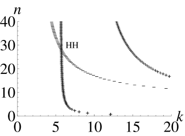
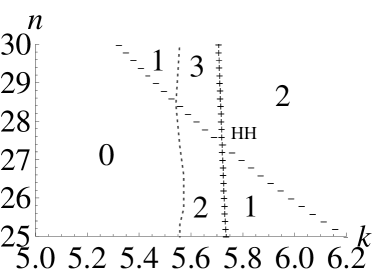
(c)                                                           (d)

Figure 4: When $\omega_{0}=3$, $\Delta=1$, $T=3$, bifurcation curves are shown in (a), with a double Hopf bifurcation labeled by HH. Near HH, number of coherent states is marked in (b). The dotted curve stands for the saddle-node bifurcation curve (sketched) illustrated in FIG. 3. “+/–” denotes subcritical/supercritical bifurcation. (c) and (d) are bifurcation curves for $T=1.15$ and $T=1$.

III.3 The case with $\tau_{0}>0$ and effect of the gap

In the rest part of this paper, we consider the case with a minimal positive delay, i.e., the case $\tau=\tilde{\tau}+\tau_{0}$ with $\tilde{\tau}$ a Gamma variable. Using the method above, we can calculate the bifurcation values. In FIG. 5 (a)–(c), we find that increasing $\omega_{0}$ will delay the occurrence of bifurcation and increase in resonant structurear9 of the dependence of $k$ on $\tau_{0}$. When $T$, the mean of Gamma distribution $\tilde{\tau}$ is larger, the effect of $\tau_{0}$ becomes weaker, thus the distributed delay $\tilde{\tau}$ acts predominantly. Increasing the variance of the natural frequency $\Delta$ even further weakens the effect of the gap $\tau_{0}$.

(a)                                                           (b)

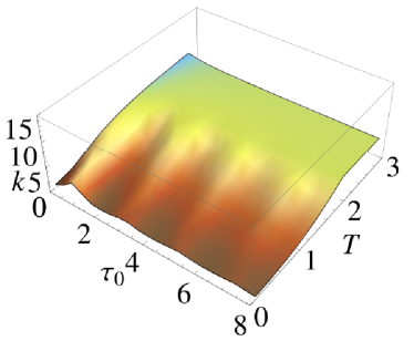
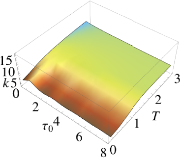
(c)                                                           (d)

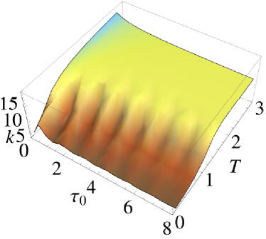
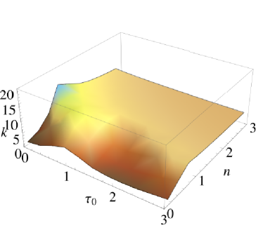
Figure 5: When $n=3$, the first bifurcation value $k$ is calculated for $(T,\tau_{0})\in[0,2.8]\times[0,8]$, (a) $\omega_{0}=3$, $\Delta=0.3$; (b) $\omega_{0}=3$, $\Delta=1$; (c) $\omega_{0}=5$, $\Delta=0.3$. (d) When $\omega_{0}=3$, $\Delta=0.3$, $T=3$, the first bifurcation value $k$ is calculated for $(n,\tau_{0})\in[0,2.8]\times[0,3]$.

(a)                                                           (b)

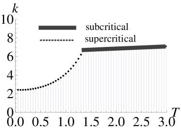
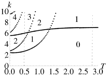
(c)                                                           (d)

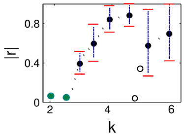
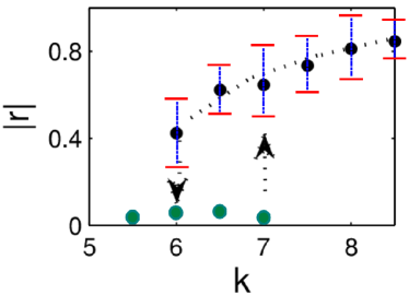
Figure 6: Fixing $\omega_{0}=3$, $\Delta=1$, $\langle\tilde{\tau}+\tau_{0}\rangle=T+\tau_{0}=3$, Var$(\tilde{\tau}+\tau_{0})=\frac{T^{2}}{n}=3$, the first bifurcation value and its direction is drawn in (a), and all bifurcation curves are illustrated in (b). The dark region stands for local stable region of incoherent state. Numbers indicates the quantity of coherent attractors. When (c) $T=0.5$($\bar{k}=2.6992$) and (d) $T=2.8$($\bar{k}=7.0388$), $|r|$ is shown in black dots by simulating system (1) with $N=128$.

By fixing $T$, we are about to consider the interactional effect of $\tau_{0}$ and the variance of Gamma distribution characterized by $n$. In FIG. 5 (d), we fix $T=3$ and investigate the effect of $\tau_{0}$ and $n$, where we find increasing $n$ will decrease in resonant structure of the dependence of $k$ on $\tau_{0}$, meanwhile weakens the effect of $\tau_{0}$.

Now we further discuss how the gap $\tau_{0}$ has an effect on the system dynamics, when fixing the mean and variance of $\tilde{\tau}+\tau_{0}$, i.e., the case shown in FIG. 1 (b). Letting $\langle\tilde{\tau}+\tau_{0}\rangle=T+\tau_{0}=3$, Var$(\tilde{\tau}+\tau_{0})=\frac{T^{2}}{n}=3$, the first Hopf bifurcation value and its direction are drawn in FIG. 6 (a). We find small $T$ (i.e., $\langle\tilde{\tau}\rangle$) makes supercritical bifurcation occur at small $k$. When $T$ is large, the subcritical bifurcation occurs at large $k$, which means that in the case of fixed mean and variance of total delay, large proportion of the gap $\tau_{0}$ (i.e., small $T$) may destroy the hysteresis loop. In FIG. 6 (b), we draw all bifurcation curves and one can also find that larger $\tau_{0}$ can significantly increase in the number of coherent attractors. When $T=0.5$ and $2.8$, respectively, simulations are carried out in FIG. 6 (c) and (d), where we find supercritical bifurcation and subcritical bifurcation in system (1) with $128$ oscillators.

To give the simulations, we first use the method in ar9 to detect the stability of incoherent state by slightly perturbing the completely incoherent state: if the incoherent state is stable we show the minimal value of $|r|$ (green dots) among 100 times of simulations with random initial values; if the incoherent state is not stable we show the average value of $|r|$ (black dots) together with error bars (red segments) over 100 times of simulations with random initial values; otherwise if the incoherent state is not always stable, which is the case of coexistence, we show the average value of $|r|$ (black dots) together with error bars (red segments) over 100 times of simulations, too, but delete these values less than 0.2. Two black circles in FIG. 6 (c) indicate speculative values of unstable coherent state bifurcating from $k=5$.

As $k$ increases, two even more Hopf bifurcations yield the coexistence of coherent states which makes the dynamical behavior more delicate. As we have seen in FIG. 6 (c), when $k>5$, the standard variance of $|r|$ among 100 times of simulations is rather large, which reveals that several stable attractors coexist. They may be originated from the second branch of Hopf bifurcation (black circles). Another reason makes this standard variance large may be the unstable hysteresis loop near $k=6$, when a subcritical bifurcation occur. When $k$ is sufficiently near this critical point, hysteresis loop no longer contains stable states, because after the first Hopf bifurcation the trivial solution of (10) is certainly unstable. Notice that this bifurcated unstable coherent state may turn into a stable one when $k$ increases far from the bifurcation point. Nevertheless, the quantity of coherent states (stable or unstable) gets larger which makes the dynamics of Kuramoto model complicated.

The effect of the gap can also be explained in the following way: we notice that in case of Gamma distribution larger $\tau_{0}$ means smaller $T$. As we have fixed the variance $\frac{T^{2}}{n}$, the excess kurtosis $\frac{6}{n}$ is larger. Notice that for Gamma distribution kurtosis and skewness obey the same monotonic dependence, thus the kurtosis can be replaced by skewness. Since excess kurtosis characterizes the sharpness of the peak of the distribution, in this point of view, larger kurtosis means that the sample data of delays are more “concentrated”, which induces a supercritical bifurcation. Similarly we conclude that decentralized samples (smaller excess kurtosis) of delay data induce subcritical bifurcations and hysteresis loop. This result is summarized from calculation results (FIG. 6 (a) and (b)). However, giving an analytical relation between bifurcation properties and kurtosis needs more derivations. This is not an easy problem, thus is left as a further work.

IV Conclusion

In this paper, we establish a normal form method by extending Nayfeh’s multiple scales to determine the properties of the bifurcated coherent states in a group of Kuramoto oscillators with heterogeneously distributed delays with a gap. Compared with the previous work niuphyd , where normal forms are derived by using a functional analysis method, we find this a simple and useful way, on the Ott-Antonsen’s manifold, to reveal the detailed dynamics near the critical values such as the direction of bifurcation, stability of bifurcated coherent states and some coexistence phenomena. They can be determined by real part of two variables $a$ and $b$.

Some numerical results indicate the effect of the gap. As direct applications of our theory, how these parameters affect system dynamics is investigated. For fixed variance and expectation of total delay, compared with the previous resultswai , we further find that larger gap $\tau_{0}$ (or larger excess kurtosis for Gamma distribution) has similar effect as the variance. It will (i) decrease the bifurcation values, (ii) induce a supercritical bifurcation hence avoid the hysteresis loop, and (iii) increase in the number of the coexisted coherent states.

- (1) Y. Kuramoto, Progr. Theoret. Phys. Suppl. 79, 223 (1984).
- (2) H. Sakaguchi, and Y. Kuramoto, Progr. Theoret. Phys. 76, 576 (1986).
- (3) Y. Kuramoto, and I. Nishikawa, J. Statist. Phys. 49, 569 (1987).
- (4) J.D. Crawford, J. Statist. Phys. 74, 1047 (1994).
- (5) Y. Kuramoto, in International Symposium on Mathematical Problems in Theoretical Physics, Lecture Notes in Physics, edited by H. Araki Springer-Verlag, Berlin, 1975 , Vol. 39.
- (6) S.H. Strogatz, Nature 410, 268 (2001).
- (7) S.H. Strogatz, Physica D 143, 1 (2000).
- (8) A. Pikovsky, M. Rosenblum, and J. Kurths, Synchronization: A Universal Concept in Nonlinear Sciences (Cambridge university press, New York, 2003).
- (9) B. Ermentrout, and T. Ko, Phil. Trans. Roy. Soc. A 367, 1097 (2009).
- (10) E.M. Izhikevich, Phys. Rev. E 58, 905 (1998).
- (11) A. Pikovsky, and M. Rosenblum, Physica D 240, 872 (2011).
- (12) J.R. Engelbrecht, and R. Mirollo, Chaos 24, 013114 (2014).
- (13) D.C. Michaels, E.P. Matyas, and J. Jalife, Circulation Res. 61, 704 (1987).
- (14) C. Liu, D.R. Weaver, S.H. Strogatz, and S.M. Reppert, Cell 91, 855 (1997).
- (15) Z. Jiang, and M. McCall, J. Opt. Soc. Am. 10, 155 (1993).
- (16) S.Yu. Kourtchatov, V.V. Likhanskii, A.P. Napartovich, F.T. Arecchi, and A. Lapucci, Phys. Rev. A 52, 4089 (1995).
- (17) K. Wiesenfeld, P. Colet, and S.H. Strogatz, Phys. Rev. E 57, 1563 (1998).
- (18) Y. Kuramoto, Chemical Oscillations, Waves, and Turbulence (Springer, Berlin, 1984).
- (19) A.T. Winfree, J. Theoret. Biol. 16, 15 (1967).
- (20) M.K. Stephen Yeung, and S.H. Strogatz, Phys. Rev. Lett. 82, 648 (1999).
- (21) S. Kim, S.H. Park, and C.S. Ryu, Phys. Rev. Lett. 79, 2911 (1997).
- (22) E. Montbrió, D. Pazó, and J. Schmidt, Phys. Rev. E 74, 056201 (2006).
- (23) S.P. Blythe, R. M. Nisbet, W.S.C. Gurney and N. Macdonald, J. Math. Anal. Appl. 109, 388–396 (1985).
- (24) J. Caperon, Ecology 50, 188–192 (1969).
- (25) W. Michiels, C.-I. Morarescu and S.-I. Niculescu, SIAM J. Control Optim., 48, 77–101 (2009).
- (26) G. Stepan, Delay-differential equation models for machine tool chatter, F.C. Moon (Ed.), Dynamics and chaos in manufacturing process, (Wiley, New York 1998).
- (27) O. Solomon and E. Fridman, Automatica 49, 3467–3475 (2013).
- (28) W.S. Lee, E. Ott, and T.M. Antonsen, Phys. Rev. Lett. 103, 044101 (2009).
- (29) E. Ott, and T.M. Antonsen, Chaos 18, 037113 (2008); Chaos 19, 023117 (2009).
- (30) Y. Yuan, and J. Bélair, SIAM J. Appl. Dyn. Syst. 10, 551 (2011).
- (31) B. Niu, and Y. Guo, Physica D 266, 23 (2014).
- (32) B. Hassard, N.D. Kazarinoff, and Y. Wan, Theory and Applications of Hopf Bifurcation (Cambridge Univ. Press, Cambridge, 1981).
- (33) T. Faria, and L. Magalhaes, J. Differ. Equations. 122, 181 (1995).
- (34) A.H. Nayfeh, Nonlinear Dynam. 51, 483 (2008).
- (35) A.H. Nayfeh, Introduction to Perturbation Techniques (Wiley, New York, 1981).
- (36) B. Niu, and W. Jiang, Nonlinear Dynam. 70, 43 (2012).
- (37) J. Hale, and S. Lunel, Introduction to Functional Differential Equations (Springer, New York, 1993).
- (38) S. Wiggins, Introduction to Applied Nonlinear Dynamical Systems and Chaos (Springer, New York, 1980).
- (39) In fact, the traditional method of multiple scales requires . In this case, one can varify .
- (40) When is in a sufficiently small neighbourhood of , the Hopf bifurcation value, the period of oscillation is given by . However, the amplitude of solutions decays very slow.
- (41) The stability can be obtained easily, by calculating the negative Floquet exponent at .
- (42) J. Wu, Trans. Amer. Math. Soc. 350, 4799 (1998).
- (43) In this case, with respect to a branch of Hopf bifurcating solutions, either it is unbounded, or it contains bifurcation points with Re at points and Re at the rest points.
- (44) J. Guckenheimer, and P. Holmes, Nonlinear Oscillations, Dynamical Systems, and Bifurcations of Vector Fields (Springer, New York 1983).