Virtual Interpolation Point Method for Viscous Flows in Complex Geometries

Abstract

A new approach for simulating flows over complex geometries is developed by introducing an accurate virtual interpolation point scheme as well as a virtual local stencil approach. The present method is based on the concept of point collocation on a virtual staggered structure together with a fractional step method. The use of a virtual staggered structure arrangement, which stores all the variables at the same physical location and employs only one set of nodes using virtual interpolation points, reduces the geometrical complexity. The virtual staggered structure consists of the virtual interpolation points and the virtual local stencil. Also, computational enhancement of the virtual interpolation point method is considerable since the present method directly discretizes the strong forms of the incompressible Navier-Stokes equations without numerical integration. It makes a key difference from others. In the virtual interpolation point method, the choice of an accurate interpolation scheme satisfying the spatial approximation in the complex domain is important because there is the virtual staggered structure for computation of the velocities and pressure since there is no explicit staggered structure for stability. In our proposed method, the high order derivative approximations for constructing node-wise difference equations are easily obtained. Several different flow problems (decaying vortices, lid-driven cavity, triangular cavity, flow over a circular cylinder and a bumpy cylinder) are simulated using the virtual interpolation point method and the results agree very well with previous numerical and experimental results. They verify the accuracy of the present method.

1 Introduction

The ability to handle complex geometries has been one of the main issue in computational fluid schemes because most engineering problems have complex geometries. So far, two kinds of grid arrangements to simulating complex flow have been known: staggered grids and non-staggered grids. For the staggered grids, vector components and scalar variables are stored at different locations, while for the non-staggered grids, vector variables and scalar variables are stored at the same locations, being half a control-volume width apart in each coordinate. Staggered grid methods are popular because of their ability to prevent checkerboard pressure in the flow solution as discussed in [1]. The main disadvantages of such an arrangement are the geometrical complexity due to the boundary conditions, and the difficulty of implementation to non-orthogonal curvilinear grids [2]. In the non-staggered grid methods, the main disadvantages are the primitive variables and mass conservation in order to solve the pressure field, either interpolation cell-face velocities or interpolate the pressure gradients in a special way, usually with an upwind-bias to avoid the checkerboard pressure fields in the flow solution.

Since most engineering problems posed on complex geometries with rough boundary pervade many fields of research(see, Figure  10), it is rather difficult for the ordinary staggered grid method or non-staggered grid method to compute the solution with numerical integration. For the purpose of numerical simplicity and efficiency, we introduce a virtual interpolation point(VIP) method using a moving least-squares(MLS) approximation without numerical integration.

Indeed, we distribute the global nodes regularly and introduce the virtual interpolation points on a local stencil(see, Figure 1). In the proposed method, the high order derivative approximations for constructing node-wise difference equations are easily obtained. Such capability allows us to get a local stencil estimate of the flux derivatives and thus preserve all complicated discontinuous behaviors of solutions. We emphasize that the mesh generation is unnecessary in our scheme and that we are convinced that our method is more effective in higher dimensions such as three-dimensional problem with a complex geometry.

Many researchers have been studying the meshfree method [3, 4, 5]. The meshfree method bases on the MLS approximation. The meshfree is attractive because it requires no connectivity among nodes in constructing approximation. Until now, however, they are prone to produce a false pressure field-checkerboard pressure. The meshfree method for hyperbolic equations has not yet been possible in literatures due to the lack of an innate dissipation mechanism essential to suppress numerical oscillations by convective terms in hyperbolic equations.

Recently, an upwind meshfree method using virtual local stencil approach was presented by Park et al [6, 7, 8], who simulated the compressible flow for the high voltage gas blast circuit breaker with the moving boundary.

1.1 The present contribution

The objective of the present study is to develop the VIP method that introduce both the virtual interpolation point and the virtual local stencil to represent properly on complex geometries. The present method is based on the MLS approach on a virtual staggered structure together with a fraction-step method. The virtual staggered structure consists of the virtual interpolation points and the virtual local stencil. It makes a key difference from others. In this implementation, the set of nodes for computation can be distributed arbitrarily in principle and hence the proposed method is applied to the flow problems on complex geometry.

The virtual local stencil(as in Park et al [6]) and the virtual interpolation points are applied only on the virtual staggered structure. A second-order accurate interpolation scheme for evaluating the virtual interpolation point is proposed in this study, which is numerically stable irrespective of the relative position between the virtual local stencil and the virtual staggered structure. It will be also shown that introduction of the virtual interpolation point is necessary to obtain physical solutions and enhance accuracy.

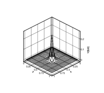
(a) $\Psi^{[0,0]}$

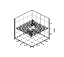
(b) $\Psi^{[1,0]}$

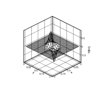
(c) $\Psi^{[0,1]}$

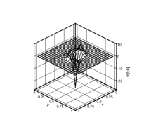
(d) $\Psi^{[2,0]}$

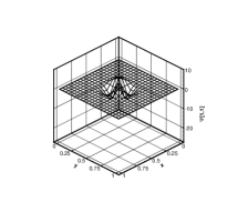
(e) $\Psi^{[1,1]}$

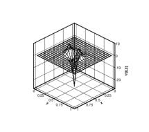
(f) $\Psi^{[0,2]}$

Figure 2: 2D $\alpha$-th shape functions with quadratic basis

In the VIP method, the high order derivative approximations for constructing node-wise difference equations are easily obtained(see, Figure 2). Also, computational enhancement is considerable since the present method directly discretizes the strong forms of incompressible Navier-Stokes equations without numerical integration.

The focus of this paper is laid on the contribution to a stable flow computation without explicit structure of staggered grid. In our method, we don’t have to explicitly construct the staggered grid at all. Instead, there exists only virtual interpolation point at each computational node, which plays a key role in discretizing the conservative quantities of the incompressible flow. In fact, it can be regarded as an imaginary staggered structure, accordingly. Particularly in our method, one set of nodes distributed on the flow domain is needed due to the virtual interpolation point.

We emphasize that the mesh and grid generation are unnecessary in our scheme and that we are convinced that our method is more effective in higher dimensions such three-dimensional problem with a complex geometry.

The reminder of the paper is organized as follows: Sections 2 and 3 present the time integration and the spatial approximation. In section 4, we propose the stable second-order VIP method for solving the incompressible Navier-Stokes equation. Various numerical results are presented to show the accuracy, efficiency, stability, and robustness and superiority of proposed scheme in Section 5. In Section 6, conclusions are drawn.

2 Governing Equations and Time Integration

The use of a virtual staggered structure arrangement, which stores all the variables at the same physical location and employs only one set of nodes using virtual interpolation points(see, Figure 1), reduces the geometrical complexity. In the present study, the VIP scheme, as in Park et al. [6, 7, 8] is applied to satisfy the continuity for the local stencil in complex domains.

The incompressible Navier-Stokes flows are represented with the following governing equations,

$$\mathbf{u}_{t}+\nabla\cdot\left(\mathbf{u}\mathbf{u}^{T}\right)+\nabla p-\frac{1}{Re}\nabla^{2}\mathbf{u} =0\;\;\;\;\textmd{on}\;\Omega,$$ (1)

$$\nabla\cdot\mathbf{u} =0\;\;\;\;\textmd{on}\;\Omega,$$ (2)

where $\mathbf{u}$ and $p$ are the velocity components and pressure of the flow. All the variables are nondimensionalized by the characteristic velocity and length scales, and $Re$ is the Reynolds number.

The time integration method used to solve Eqs.(1) and (2) is based on a fractional step method where a pseudo-pressure is used to correct the velocity field so that the continuity equation is satisfied at each computational time step. In this study, we use a second-order semi-implicit time advancement scheme (a second-order Adams-Bashforth for the convection terms and a second-order Crank-Nicolson method for the diffusion terms)

$$\mathbf{Au}^{\star}=\mathbf{r}^{n},$$ (3)

$$\Delta\phi^{n+1}=\frac{1}{\triangle t}\nabla\cdot\mathbf{u}^{\star},$$ (4)

$$\mathbf{u}^{n+1}=\mathbf{u}^{\star}-(\triangle t)\nabla\phi^{n+1},$$ (5)

$$p^{n+1} =p^{n}+\phi^{n+1}-\frac{\triangle t}{2Re}\Delta\phi^{n+1},$$ (6)

where

$$\mathbf{A} =\frac{1}{\triangle t}\left(\mathbf{I}-\frac{\triangle t}{2Re}\Delta\right),$$

$$\mathbf{r}^{n} =\frac{1}{\triangle t}\left(\mathbf{I}+\frac{\triangle t}{2Re}\Delta\right)\mathbf{u}^{n}-\left[\nabla\cdot\left(\mathbf{uu}^{T}\right)\right]^{n+\frac{1}{2}},$$

$\mathbf{u}^{\star}$ is the intermediate velocity, and $\phi$ is the pseudo-pressure. Also, $\triangle t$ and $\mathbf{I}$ are the computational time step and the identity operator.

In the present study, the VIP method is applied to Cartesian coordinate. The time-integration method is based on the method of Kim and Moin [9] to enhance computational efficiency.

3 Moving Least-Squares Approximation

For spatial approximation of solutions, the MLS approximation in the literature [3] is employed. We briefly explain the MLS approximation.

For simplicity, we just consider 2-dimensional space and take $m=2$ but it can be extended to $n$-dimension. Multi-index notations are adapted throughout the paper

$$\mathbf{x}=(x,y)\textmd{ and }\partial^{\mathbf{(\alpha},\beta)}_{\mathbf{x}}=\partial_{x}^{\alpha}\partial_{y}^{\beta},$$

where $\alpha$ and $\beta$ are non-negative integers. For a continuous function $u(\mathbf{x})$ we can approximate this function at a point $\bar{\mathbf{x}}=(\bar{x},\,\bar{y})$ in terms of polynomials up to some order dependently on a neighborhood of $\bar{\mathbf{x}}$, which is found by Weierstass.

Let $u_{m}(\mathbf{x},{\bar{\mathbf{x}}})$ be a polynomial up to degree $m$ which depends on the point $\bar{\mathbf{x}}$. Then for some coefficient vectors $\mathbf{c}$, it can be assumed that

$$u_{m}(\mathbf{x},{\bar{\mathbf{x}}}) =\mathbf{c}_{1}(\bar{\mathbf{x}})+\left(\frac{x-\bar{x}}{\rho(\bar{\mathbf{x}})}\right)\mathbf{c}_{2}(\bar{\mathbf{x}})+\left(\frac{y-\bar{y}}{\rho(\bar{\mathbf{x}})}\right)\mathbf{c}_{3}(\bar{\mathbf{x}})$$

$$+\left(\frac{x-\bar{x}}{\rho(\bar{\mathbf{x}})}\right)^{2}\mathbf{c}_{4}(\bar{\mathbf{x}})+\left(\frac{x-\bar{x}}{\rho(\bar{\mathbf{x}})}\right)\left(\frac{y-\bar{y}}{\rho(\bar{\mathbf{x}})}\right)\mathbf{c}_{5}(\bar{\mathbf{x}})+\left(\frac{y-\bar{y}}{\rho(\bar{\mathbf{x}})}\right)^{2}\mathbf{c}_{6}(\bar{\mathbf{x}}).$$

The dilation function $\rho(\bar{\mathbf{x}})$ can be regarded as the size of a neighborhood at $\bar{\mathbf{x}}$ for approximation.

In order to find the best approximation $u_{m}(\mathbf{x},{\bar{\mathbf{x}}})$ with the coefficient $\mathbf{c}(\bar{\mathbf{x}})$, we define the locally weighted square functional of the form on a given set of nodes, $\Lambda=\{\mathbf{x}_{i}\in\bar{\Omega}|i=1,2,\cdots,N\}$.

$$J(\mathbf{c}(\bar{\mathbf{x}}))=\sum_{i=1}^{N}\Phi\left(\frac{\mathbf{x}-\bar{\mathbf{x}}}{\rho(\bar{\mathbf{x}})}\right)|{u_{m}(\mathbf{x}_{i},{\bar{\mathbf{x}}})-u(\mathbf{x}_{i})}|^{2}$$

where the weight function is taken as the following form,

$$\Phi\left(\mathbf{y}\right)=\left\{\begin{array}[]{ll}\left(1-\|\mathbf{y}\|^{\left(1-\|\mathbf{y}\|\right)^{2}}\,\right)^{4},&\quad if\quad\|\mathbf{y}\|<1\\ 0\quad\quad\quad\quad\quad\quad\quad\quad,&\quad otherwise.\\ \end{array}\right.$$

Minimizing the functional $J$, the local approximation $u_{m}(\mathbf{x},{\bar{\mathbf{x}}})$ is determined with coefficient $\mathbf{c}(\bar{\mathbf{x}})$. In fact, it is the best approximation, partially near $\bar{\mathbf{x}}$. Moreover, $u_{m}$ is a polynomial is $\mathbf{x}$, so that we can differentiate it as many times as we want. It is also natural that the derivative of $u_{m}(\mathbf{x},{\bar{\mathbf{x}}})$ w.r.t. $\mathbf{x}$ are good approximate of derivatives. Therefore, we pay our attention to the values of $u_{m}(\mathbf{x},{\bar{\mathbf{x}}})$ and its derivatives at $\bar{\mathbf{x}}$. This observation produces the following approximates,

$$\left(\mathcal{D}^{[\alpha,\beta]}u\right)(\bar{\mathbf{x}})\equiv\lim_{\mathbf{x}\rightarrow\bar{\mathbf{x}}}\partial^{(\alpha,\beta)}_{\mathbf{x}}u_{m}(\mathbf{x},{\bar{\mathbf{x}}}).$$

Following the above procedure, we finally have the representation formula for approximated derivatives,

$$\left(\mathcal{D}^{[\alpha,\beta]}u\right)(\bar{\mathbf{x}})=\sum_{i=1}^{N}u(\mathbf{x}_{i})\Psi^{[\alpha,\beta]}_{i}(\bar{\mathbf{x}}),$$ (7)

in which we call $\Psi^{[\alpha,\beta]}_{i}(\bar{\mathbf{x}})$ the $[\alpha,\beta]$-th approximative of a shape function at $\bar{\mathbf{x}}_{i}$. For detailed description, see the reference [3].

4 Implementation using Virtual Interpolation Point

Using the conventional MLS approximations only, we have empirically experienced that the fractional step method becomes unstable. This is why we elaborate the VIP scheme on a virtual local stencil for stability.

The VIP method is developed for the solution of computational fluid dynamics problems that does not require the use of staggered grid systems. This implementation of this scheme is performed on only one set of nodes for both velocities and pressure. It makes a key difference from others. In this implementation, the set of nodes for computation can be distributed arbitrarily in principle and hence the proposed method can be applied to the flow problems on complicated geometry.

4.1 Numerical Flux using the VIPs on a Local Stencil

The key idea of VIP scheme is that conservative variables are obtained by the conventional MLS approximation at the auxiliary virtual interpolation points, which are not necessary nodes. In the present method, the choice of an accurate interpolation scheme satisfying the spatial approximation in the complex domain is important because there is the virtual staggered structure for computation of the velocities and pressure but there is no explicit staggered structure for stability. In the proposed method, the high order derivative approximations for constructing node-wise difference equations are easily obtained.

We first introduce the approximations of the identity and Laplacian operators,

$$\mathbf{I}=\mathcal{D}^{[0,0]}\textrm{ and }\Delta=\mathcal{D}^{[2,0]}+\mathcal{D}^{[0,2]},$$ (8)

using the MLS approximations in (7). The Laplacians in (3), (4),and (6) are all replaced with the operator in (8). In addition, every variable without differential operators is approximated through the identity operator.

$\left[\nabla\cdot\left(\mathbf{u}\mathbf{u}^{T}\right)\right]^{n+1/2}$ is the non-linear convection term at node $\mathbf{x}$. Implicitly handling viscous term eliminates the numerical instability due to the CFL restriction. The term $\left[\nabla\cdot\left(\mathbf{u}\mathbf{u}^{T}\right)\right]^{n+1/2}$ is approximated in a second-order temporal approximation for the convective derivative term at time level $t_{n+1/2}$ which is usually called Adams-Bashforth,

$$\left[\nabla\cdot\left(\mathbf{u}\mathbf{u}^{T}\right)\right]^{n+1/2}=\frac{1}{2}\left[3\nabla\cdot\left(\mathbf{u}^{n}\left(\mathbf{u}^{n}\right)^{T}\right)-\nabla\cdot\left(\mathbf{u}^{n-1}\left(\mathbf{u}^{n-1}\right)^{T}\right)\right]+O(\Delta t^{2}).$$

Second, instead of directly applying the derivative approximations in MLS approximation to the convective terms, we simply take the direct difference for implementing the divergence operator as in the finite difference method. Let ${\mathbf{x}}_{e},{\mathbf{x}}_{w},{\mathbf{x}}_{s},$ and ${\mathbf{x}}_{n}$ denote east, west, south, and north points from the node $\mathbf{x}_{i}$ on the local stencil in Fig. 1. We call these points the virtual interpolation points of $\mathbf{x}_{i}$. When $\mathbf{x}_{i}$ is far away from the boundary, it is not difficult to choose the virtual interpolation points around $\mathbf{x}_{i}$. However, technical problem can happen in case where the node $\mathbf{x}_{i}$ is close to the boundary of the computational domain.

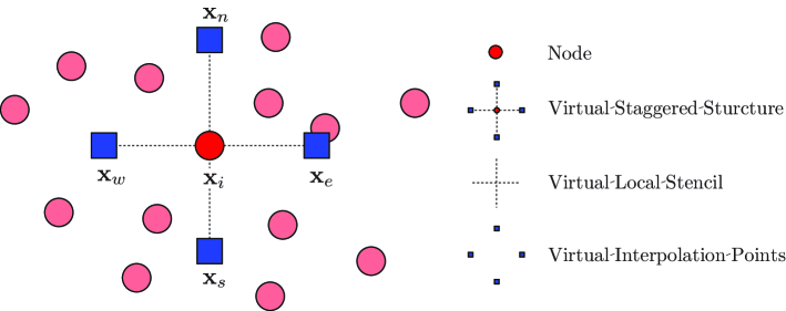
Figure 1: Schematic diagram for virtual interpolation points on the local stencil at a node $\mathbf{x}_{i}\in\Lambda$.

Three conservative terms under consideration are, $\nabla\cdot\left(\mathbf{uu}^{T}\right)$ appearing in $\mathbf{r}^{n}$ in (3), $\nabla\cdot\mathbf{u}$ in (4), and, $\nabla\phi$ in (5). At each interior node $\mathbf{x}_{i}\in\Omega\cap\Lambda$, the following discretizations are used for the local conservation over a local stencil consisting to the virtual interpolation points at node $\mathbf{x}_{i}\in\Omega\cap\Lambda$;

1. Convection Term using the VIPs on the Virtual Local Stencils

   $$\nabla\cdot\left(\mathbf{u}\mathbf{u}^{T}\right)\bigg{|}_{\textbf{x}_{i}} \approx\left(\begin{array}[]{c}\frac{u^{2}({\mathbf{x}}_{e})-u^{2}({\mathbf{x}}_{w})}{\|{\mathbf{x}}_{e}-{\mathbf{x}}_{w}\|}+\frac{u({\mathbf{x}}_{n})\,v({\mathbf{x}}_{n})-u({\mathbf{x}}_{s})\,v({\mathbf{x}}_{s})}{\|{\mathbf{x}}_{n}-{\mathbf{x}}_{s}\|}\\ \frac{u({\mathbf{x}}_{e})\,v({\mathbf{x}}_{e})-u({\mathbf{x}}_{w})\,v({\mathbf{x}}_{w})}{\|{\mathbf{x}}_{e}-{\mathbf{x}}_{w}\|}+\frac{v^{2}({\mathbf{x}}_{n})-v^{2}({\mathbf{x}}_{s})}{\|{\mathbf{x}}_{n}-{\mathbf{x}}_{s}\|}\\ \end{array}\right),$$

   where

   $$\mathbf{u}(\mathbf{x}_{{}_{vip}})=\sum_{i=1}^{N}\Psi^{[0,0]}_{i}(\mathbf{x}_{{}_{vip}})\mathbf{u}_{i},\quad vip=e,w,n,s,$$

2. Divergence Term using the VIPs on the Virtual Local Stencils

   $$\nabla\cdot\left(\mathbf{u}^{\star}\right)\bigg{|}_{\textbf{x}_{i}} \approx\begin{array}[]{c}\frac{u^{\star}({\mathbf{x}}_{e})-u^{\star}({\mathbf{x}}_{w})}{\|{\mathbf{x}}_{e}-{\mathbf{x}}_{w}\|}+\frac{v^{\star}({\mathbf{x}}_{n})-v^{\star}({\mathbf{x}}_{s})}{\|{\mathbf{x}}_{n}-{\mathbf{x}}_{s}\|},\\ \end{array}$$

   where

   $$\mathbf{u}^{\star}(\mathbf{x}_{{}_{vip}})=\sum_{i=1}^{N}\Psi^{[0,0]}_{i}(\mathbf{x}_{{}_{vip}})\mathbf{u}^{\star}_{i},\quad vip=e,w,n,s,$$

3. Gradient Term using the VIPs on the Virtual Local Stencils

   $$\nabla\phi\bigg{|}_{\textbf{x}_{i}} \approx\left(\begin{array}[]{c}\frac{\phi({\mathbf{x}}_{e})-\phi({\mathbf{x}}_{w})}{\|{\mathbf{x}}_{e}-{\mathbf{x}}_{w}\|}\\ \frac{\phi({\mathbf{x}}_{n})-\phi({\mathbf{x}}_{s})}{\|{\mathbf{x}}_{n}-{\mathbf{x}}_{s}\|}\\ \end{array}\right),$$

   where

   $$\phi(\mathbf{x}_{{}_{vip}})=\sum_{i=1}^{N}\Psi^{[0,0]}_{i}(\mathbf{x}_{{}_{vip}})\phi_{i},\quad vip=e,w,n,s.$$

5 Numerical experiments

In this section, several different flow problems (Decaying vortices, lid-driven cavity flow, triangular cavity flow, flow over a circular cylinder and a bumpy circular cylinder) are simulated using the VIP method proposed in this study and the results agree very well previous numerical and experimental results, verifying the accuracy of the present method.

5.1 Taylor decaying vortices

The temporal and spatial accuracy of the VIP method is verified by simulating the two-dimensional unsteady flows such as

$$u(x,y,t) =-\cos x\sin ye^{-2t},$$

$$v(x,y,t) =\sin x\cos ye^{-2t},$$

$$p(x,y,t) =-\frac{1}{4}\left[\cos 2x+\cos y\right]e^{-4t}.$$

We consider the Taylor decaying vortices on the domain $\Omega=(0,\pi)\times(0,\pi)$, which is discretized with regular nodes.

As shown in the Fig. 3, we have obtained the convergence results of $O(h^{2})$ and $O(\Delta t^{2})$ for the temporal and spatial on uniform nodes, respectively.

(a) $\Delta t=10^{-4}.$

(b) $h=\pi/320$.

Figure 3: Error convergence plots of Taylor decaying vortex: (a) Spatial of the VIP method evaluated using the unsteady Navier-Stokes Taylor vortex analytical solution at t = 0.1; (b) Temporal accuracy of the VIP method evaluated using the unsteady Navier-Stokes Taylor vortex analytical solution at t = 1.0.

5.2 Lid-driven cavity flow

This classical problem has become a standard benchmark for assessing the performance of algorithms for the incompressible Navier-Stokes equations. For a typical example of the interior flow with corner singularity, many researchers have extensively studied the square cavity flow on a unit square domain to access the accuracy of the numerical solution. The $u$-velocity on the vertical center line $x=0.5$ and the $v$-velocity on the horizontal center line $y=0.5$ are given in Fig. 4d. For each sectional velocity, typical regular(see, Figures 4a - 4c) distributed nodes are, respectively, employed for comparison purpose. It is shown that all the results obtained from the VIP method are in good agreement with the data by Giha et al. [10] which ha been a widely accepted reference for the validation.

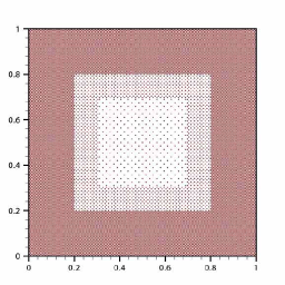
(a) 22,925 nodes

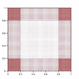
(b) 12,048 nodes

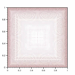
(c) 7,897 nodes

Figure 4: Cavity flow: (a), (b), and (c) are various regular distributed nodes(a-c); (d) velocity profiles along middle sections for the various regular nodes of the square cavity problem $Re$=1000.

5.3 Triangular cavity flow

The two-dimensional steady incompressible flow inside a triangular driven cavity is also an interesting subject like the square driven cavity flow. This flow was studied analytically by Moffatt [11] in the Stokes regime. Moffatt showed that the intensities of eddies and the distance of eddy centers from the corner, follow a geometric sequence.

We apply the VIP method to this Moffatt eddy simulation for the flow in a wedge-shaped domain(see, Figure 5). In the velocity profile, the points where the $u$-velocity has local maximum correspond to the $u$-velocity at the dividing streamline between the eddies, where Moffatt have used these velocities as a measure of the intensity of consecutive eddies. Table 1 and  2 tabulate the calculated ratios of $r_{n}/r_{n+1}$ and $I_{n}/I_{n+1}$ for isosceles triangle with $\theta=28.072^{\circ}$ along with analytical predictions of Moffatt and the agreement is good. The contour lines for u-velocity, v-velocity, pressure, stream function, and vorticity are shown in Fig. 6 where the sequence of eddies is well presented. The changing signs of the velocity components are properly illustrated toward the vertex of the wedge, which causes the small eddies.

	$r_{1}/r_{2}$	$r_{2}/r_{3}$	$r_{3}/r_{4}$	$r_{4}/r_{5}$	$r_{5}/r_{6}$
VIP method($400\times 800/2$)	1.99	2.01	2.01	2.00	1.96
Moffatt [11]	$r_{n}/r_{n+1}=2.01$

Table 1: Relative eddy center locations $r_{n}/r_{n+1}$ for isosceles triangle with $\theta=28.072^{\circ}$

	$I_{1}/I_{2}$	$I_{2}/I_{3}$	$I_{3}/I_{4}$	$I_{4}/I_{5}$	$I_{5}/I_{6}$
VIP method($400\times 800/2$)	385.7	406.0	402.3	388.1	380.9
Moffatt [11]	$I_{n}/I_{n+1}=407$

Table 2: Relative eddy center intensities $I_{n}/I_{n+1}$ for isosceles triangle with $\theta=28.072^{\circ}$

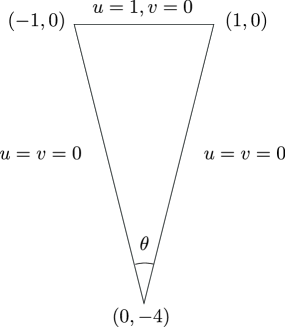
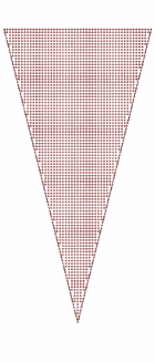
Figure 5: Isosceles triangle cavity flow with $\theta=28.072^{\circ}$ : (a) Problem description; (b) regular distributed nodes.

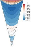
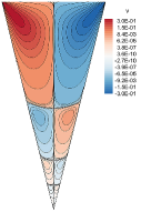
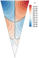
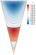
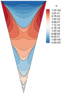
Figure 6: Moffatt eddies toward the vertex of an isosceles triangle with $\theta=28.072^{\circ}$ : (a) $u$-velocity; (b) $v$-velocity; (c) pressure; (d) stream function; (e) vorticity.

5.4 Flow past a circular cylinder: Steady and Unsteady

Flow past a circular cylinder is one of the classical problems of fluid mechanics. For lower value of Reynolds number, the flow is steady and symmetric. And as the Reynolds number is increased, the flow past a circular cylinder is a problem unsteady in nature and, therefore, good numerical accuracy is required in order to capture the different phenomena present in the evolving solution.

To validate the VIP scheme, the numerical simulation of the steady and unsteady flows past a circular cylinder is carried out. In the problem under investigation, depicted in Fig. 7 along with the computational domain and the distributed nodes. The Reynolds number in the this flow is defined as $Re=u_{\infty}D/\nu$ where $D$ is the diameter of the cylinder. We impose $u$ = 1 and $v$ = 0 for inlet, and traction free condition, $(t_{x},t_{y})$ = 0 for outlet, and $v$ = 0 and $t_{x}$ = 0 for top and bottom boundary. The traction vector $\bf{t}$ is defined by $\mathbf{t}=-p\mathbf{n}+\nu\partial\mathbf{u}/\partial\mathbf{n}$ with $\mathbf{n}$ denoting the outward normal. At low Reynolds numbers, the flow develops two symmetric wakes past the cylinder. This solution becomes unstable for Reynolds numbers over $40$, and periodic vortex shedding appears. These vortices are transported by the flow, creating what is known in the literature as Von Karman vortex street.

Figure 8 shows the spanwise vorticity contours for $Re=40$ and $Re=100$. Table 3 and Figure 9 show the results of simulations together with the previous numerical results of Takami et al. [12] and H. Ding [13], where $C_{D}$ is the drag coefficient(time-averaged value in case of $Re$=100) and $C^{\prime}_{L}$ is the amplitude of lift-coefficient fluctuations (maximum deviation from the time-averaged value) at $Re$=100. The Strouhal number ($St=fd/u_{\infty}$) is also in excellent agreement with numerical results(see, Table 3 and Figure 9).

		$Re$		$C_{D}$		$C^{{}^{\prime}}_{L}$		$St$
VIP method		40		1.536
		100		1.328		$\pm$ 0.31		0.164
Takami et al. [12]		40		1.536
H. Ding [13]		100		1.325		$\pm$ 0.28		0.164

Table 3: Simulation results for flow over a circular cylinder.

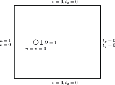
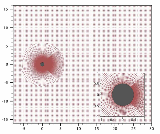
Figure 7: Flow past a circular cylinder : (a) Problem description; (b) regular distributed nodes and close-up of the central block containing the cylinder.

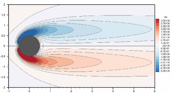
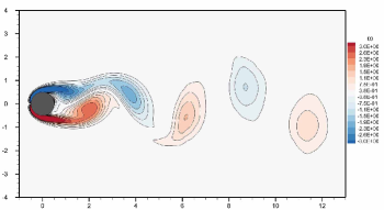
Figure 8: Spanwise vorticity contours near a circular cylinder : (a) $Re$ = 40; (b) $Re$ = 100, instantaneous vorticity contours are drawn.

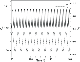
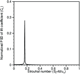
Figure 9: Results of flow past a circular cylinder with $Re=100$: (a) Temporal evolution of lift coefficient and drag coefficient; (b) Normalized power spectral density (PSD) for lift coefficient. The Strouhal number ($S_{t}$) is indicated by the summit of the curve ($S_{t}=0.164)$).

5.5 Flow past a bumpy circular cylinder

Analytic solutions are rarely available, and conventional numerical computations are usually out of reach since the rapidly varying wrinkles and the domain have different length scales. The traditional remedy is to pose special boundary conditions on a mollified domain to capture the geometrical influence of the wrinkles. The development of such conditions is cumbersome in general, and modeling error estimates can be out of reach.

Nevertheless, many problems involving oscillating boundaries or interfaces arise in many fields of physics and engineering sciences, such as the scattering of acoustic waves on small periodic obstacles, the free vibrations of strongly nonhomogeneous elastic bodies, the behavior of fluids over rough walls.

Interesting example in the fluid mechanics is the flow field around golf balls, in which the wrinkles associated to the curvature decrease the gap between the air-pressure behind and in front of the ball.

As depicted below, we represent the surface by a bumpy circle $\textbf{x}(\theta)$ of which the radial deviation is introduced by the following sinusoidal curves:

$$\textbf{x}(\theta) =r\left[1+\gamma\cos(m_{b}\theta)\right](\cos\theta,\sin\theta),$$

where $r$ is a dimensionless average radius of the bumpy circle, $\gamma$ denotes the amplitude ratio of a bump, and $m_{b}$ is the total number of bumps along the circumference. $r$=0.5, $\gamma$=0.1 and $m_{b}=10,20,30,\cdots,90,100$ are used in our simulations(see, Figure 10). The present method never employs any meshes, grids, or even integration cells, i.e., being entirely free from connectivity data. Thus it has an advantage over other numerical methods that are based on subdivisions in modelling this complex geometry of bumpy circular cylinder, as can be noticed from (b) in Fig. 11. Stepwise adaptive node distribution is also employed similarly as introduced in the previous example of flow around a circular cylinder. For all cases, we use a fixed value of $Re=40$. Stepwise adaptive node distribution is also employed similarly as introduced in the previous example of flow around a circular cylinder.

The aim of this example is to investigate the correlation between the drag coefficient and the shape of bumpy circles. With the increase of bumpy numbers, $m_{b}$, we calculate the drag coefficients given by

$$C_{D}=\frac{F_{D}}{U^{2}R},$$

where $F_{D}$ is the drag force, $U$ is the characteristic velocity ($U$=1), and the maximum radius $R$ is the characteristic length($R$=0.55).

Drag reduction via altering the no-slip condition, often achieved through microgeometries or micro-patterning which trap the fluid, is a topic that has received attention over the years. This reduction, known as the roller bearing effect, is due to the formation of embedded vortices within the bumps(or triangular cavities).

Several interesting trends are found in our results. First of all, the changes of drag coefficients are noticeable as the number of bumps increases. Drag data was then compared to that obtained over a regular smooth circular cylinder. The result of drag coefficients($C_{D}$) are presented in Fig. 15(a). The coefficient of total drag increases until $m_{b}$ reaches 30. Then, after $m_{b}$=30, the total drag coefficient decreases back. Exceeding $m_{b}$ = 100, the coefficient becomes far less than the reference value that is the case of the regular smooth circle of the radius $R$ and is plotted on the vertical axis in the figure. Results show that for $m_{b}>30$ an appreciable drag reduction of greater than 7.9% is obtained.

We also show the dependence of form drag and viscous drag on the bump number in Fig. 15(b). It is as well of interesting note that the viscous drag coefficient decreases as the number of bumps increases. It keeps decreasing down to less than 80% lesser value than that of the regular circle ($m_{b}=0$).

The flow pattern is illustrated in Figs. 12, 13, and 14 for the cases of $m_{b}$ = 10, 30, 50, 70, 90, 100. In figure. 12, the lines do not depict equal intervals, which is intended to visualize the weak eddies arising between bumps. These eddies may implicate the energy transfer from flow and, as a result, the drag on the body. In order to further convince ourselves, we show the values of pressure($C_{p}$) profiles along the surfaces are given in Fig. 16 for three different numbers of bumps, $m_{b}$ =10, 30, and 100. The pressure profiles vary up and down along the circumference, being consistent with the each bumpy shape considered.

The bumpy circular cylinders are able to reduce the total drag in a viscous flow via an embedded vortex inside of the bumps that imposes a slip condition, versus a no-slip condition, where the bottom wall in a viscous flow would normally be. Increased aspect ratio and reduced gap height lead to better drag reduction potential at Reynolds number,$Re=$40.

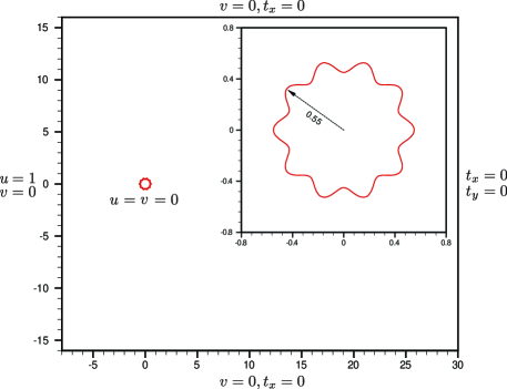
(a) $m_{b}=10$.

(b) $m_{b}=20$.

(c) $m_{b}=30$.

(d) $m_{b}=40$.

(e) $m_{b}=50$.

(f) $m_{b}=60$.

(g) $m_{b}=70$.

(h) $m_{b}=80$.

(i) $m_{b}=90$.

(j) $m_{b}=100$.

Figure 10: The numerical setting for flow past various bump cylinders: (a) the computational domain with the external dimension of $(-8,30)\times(-16,16)$; (b)-(k) are various shape of bumpy circles.

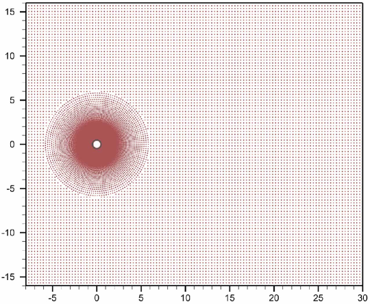
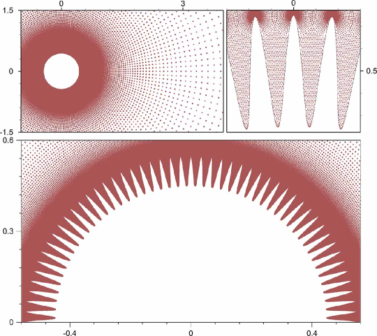
(a) $m_{b}=100$

Figure 11: The numerical feather for flow past a bumpy cylinder($m_{b}$=100): (a) the node distribution($236,604$ nodes) of the full domain for the computations of the external flow; (b) the close up and the zoom-in views of the bumpy circle and the radial stepwise uniform node distribution with the radius of R=0.55

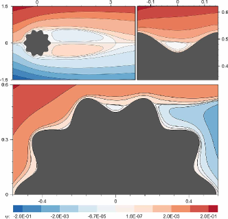
(a) $m_{b}=10$

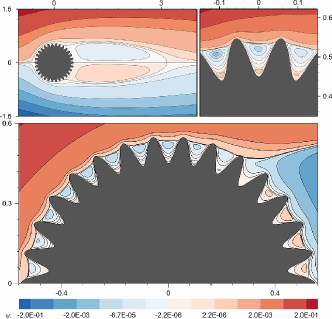
(b) $m_{b}=30$

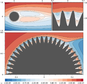
(c) $m_{b}=50$

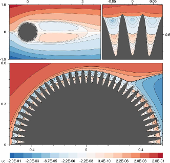
(d) $m_{b}=70$

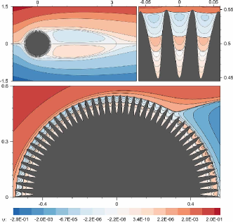
(e) $m_{b}=90$

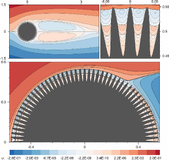
(f) $m_{b}=100$

Figure 12: Flow pattern around various bumpy circular cylinders with $Re=40$. The stream function contours around the body for six different numbers of bumps, $m_{b}$ = 10, 30, 50, 70, 90, and 100.

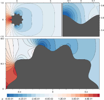
(a) $m_{b}=10$

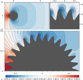
(b) $m_{b}=30$

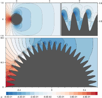
(c) $m_{b}=50$

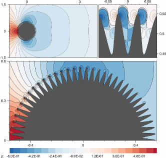
(d) $m_{b}=70$

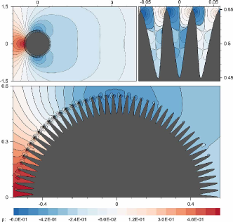
(e) $m_{b}=90$

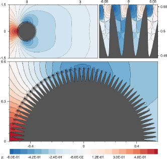
(f) $m_{b}=100$

Figure 13: Flow pattern around various bumpy circular cylinders with $Re=40$. The pressure contours around the body for six different numbers of bumps, $m_{b}$ = 10, 30, 50, 70, 90, and 100.

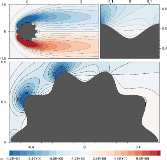
(a) $m_{b}=10$

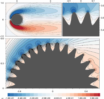
(b) $m_{b}=30$

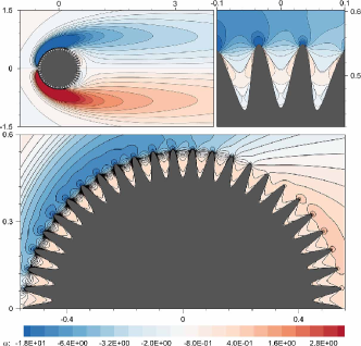
(c) $m_{b}=50$

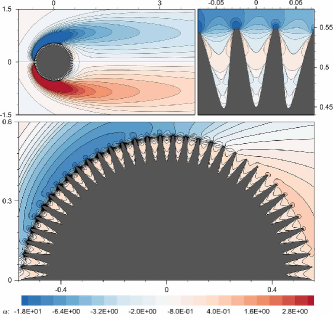
(d) $m_{b}=70$

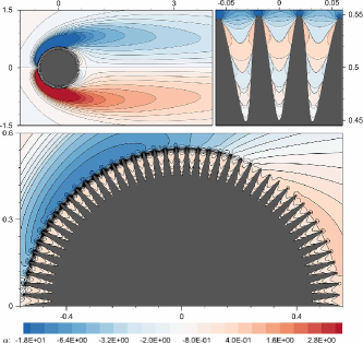
(e) $m_{b}=90$

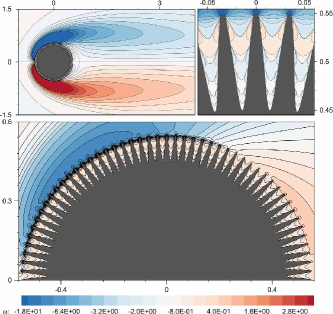
(f) $m_{b}=100$

Figure 14: Flow pattern around various bumpy circular cylinders with $Re=40$. The vorticity contours around the body for six different numbers of bumps, $m_{b}$ = 10, 30, 50, 70, 90, and 100.

Figure 15: Dependence of drag coefficients on the number of bumps with $Re=40$: (a) total Drag; (b) viscous drag and form drag. Three values on the vertical axis are the drag coefficients calculated in the reference case where the regular smooth circle of the radius $R=0.55$ is employed.

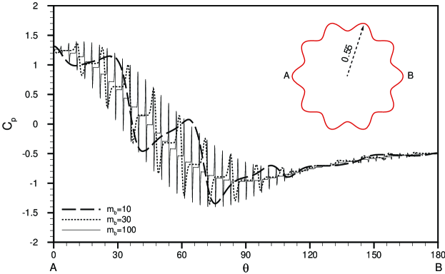
Figure 16: Pressure distributions on the bumpy surface with $Re=40$. A and B indicate the front and end noses.

6 Conclusion

In this study, a new VIP method is presented by introducing the accurate virtual interpolation point scheme as well as the virtual local stencil approach. The present method is based on the concept of point collocation on a virtual staggered structure together with a fractional step method.

The virtual staggered structure consists of the virtual interpolation points and the virtual local stencil. The use of the virtual staggered structure arrangement, which stores all the variables at the same physical location and employs only one set of nodes using virtual interpolation points, reduces the numerical difficulty is caused by geometrical complexity.

In the VIP method, the choice of an accurate interpolation scheme satisfying the spatial approximation in the complex domain is important because there is the virtual staggered structure for computation of the velocities and pressure since there is no explicit staggered structure for stability. In our proposed method, the high order derivative approximations for constructing node-wise difference equations are easily obtained.

Several different flow problems (decaying vortices, lid-driven cavity, triangular cavity, flow over a circular cylinder and a bumpy cylinder) are simulated using the virtual interpolation point method proposed in this study. The simulation results with both the the accurate virtual interpolation point scheme and the virtual local stencil approach agree very well with the previous numerical and experimental results, indicating the validity and accuracy of the present VIP method.

References

- Patankar [1980] S. V. Patankar, Numerical heat transfer and fluid flow, Hemisphere Pub. Corp., Washington, D.C., New York, 1980.
- Peric [1985] M. Peric, A finite volume method for the prediction of three-dimensional fluid flow in complex ducts, Ph.D. thesis, London University, London, UK, 1985.
- Kim and Kim [2003] D. W. Kim, Y. Kim, Point collocation methods using the fast moving least-square reproducing kernel approximation, Int. J. Numer. Methods Eng. 56 (2003) 1445–1464.
- Kim et al. [2001] Y. Kim, D. Kim, H. Kim, H. J. Choe, Meshless method for the stationary incompressible Navier-Stokes equations, Discret. Contin. Dyn. Syst. - Ser. B 1 (2001) 495–526.
- Choe et al. [2006] H. J. Choe, Y. Kim, D. W. Kim, Meshfree method for the non-stationary incompressible Navier-Stokes equations, Discret. Contin. Dyn. Syst. - Ser. B 6 (2006) 17–39.
- Park et al. [2007] S.-K. Park, K.-Y. Park, H. J. Choe, Flow field computation for the high voltage gas blast circuit breaker with the moving boundary, Comput. Phys. Commun. 177 (2007) 729–737.
- Choe et al. [2006] H. J. Choe, M.-Y. Ahn, K. D. Song, K.-Y. Park, S.-K. Park, Flow Field Computation for Simplified High Voltage Gas Circuit Breaker Model by Upwind Meshfree Method, Jpn. J. Appl. Phys. 45 (2006) 9247–9253.
- Park [2010] S.-K. Park, Flow field computation of compressible Euler equations in time varying domain, Ph.d thesis, Yonsei University, Seoul, Korea, 2010.
- Kim and Moin [1985] J. Kim, P. Moin, Application of a fractional-step method to incompressible Navier-Stokes equations, J. Comput. Phys. 59 (1985) 308–323.
- Ghia et al. [1982] U. Ghia, K. Ghia, C. Shin, High-Re solutions for incompressible flow using the Navier-Stokes equations and a multigrid method, J. Comput. Phys. 48 (1982) 387–411.
- Moffatt [2006] H. K. Moffatt, Viscous and resistive eddies near a sharp corner, J. Fluid Mech. 18 (2006) 1.
- Takami [1969] H. Takami, Steady Two-Dimensional Viscous Flow of an Incompressible Fluid past a Circular Cylinder, Phys. Fluids 12 (1969) II–51.
- Ding et al. [2004] H. Ding, C. Shu, K. Yeo, D. Xu, Simulation of incompressible viscous flows past a circular cylinder by hybrid FD scheme and meshless least square-based finite difference method, Comput. Methods Appl. Mech. Eng. 193 (2004) 727–744.