Moment bounds in spde’s with application to the stochastic wave equation

1 Introduction

Consider a partial differential operator $\mathcal{L}$ in the time and space variables $(t,x)$ and a space-time white noise $\dot{W}(t,x)$, where $t\in\mathbb{R}_{+}^{*}=\mathbb{R}_{+}\setminus\{0\}$ and $x\in\mathbb{R}^{d}$, along with a function $\theta(t,x)$. We are interested in determining when the stochastic partial differential equation (spde)

$$\mathcal{L}u(t,x)=\rho\left(u(t,x)\right)\theta(t,x)\dot{W}(t,x)\;,\qquad x\in\mathbb{R}^{d},\;t\in\mathbb{R}_{+}^{*}\;,$$ (1.1)

with appropriate initial conditions, admits as solution a random field $(u(t,x),\ (t,x)\in\mathbb{R}_{+}\times\mathbb{R}^{d})$. In this case, we would like estimates and asymptotic properties of moments of $u(t,x)$, as well as Hölder-continuity properties. In this paper, we will develop such estimates for a wide class of operators $\mathcal{L}$, functions $\theta$ and initial conditions, with an emphasis on the stochastic wave and heat equations.

One basic example, which also was the starting point of this study, is the parabolic Anderson model. In this case, $d=1$, $\mathcal{L}=\frac{\partial}{\partial t}-\kappa^{2}\frac{\partial^{2}}{\partial x^{2}}$, $\rho(x)=\lambda x$ and $\theta\equiv 1$. The intermittency property of this equation, as defined in [7], is studied via the moment Lyapounov exponents, in which estimates of the moments play a key role. Indeed, recall that the upper and lower moment Lyapunov exponents for constant initial data are defined as follows:

$$\overline{m}_{p}(x):= \mathop{\lim\sup}_{t\rightarrow+\infty}\;\frac{\log\mathbb{E}\left[|u(t,x)|^{p}\right]}{t},\qquad\underline{m}_{p}(x):=\mathop{\lim\inf}_{t\rightarrow+\infty}\;\frac{\log\mathbb{E}\left[|u(t,x)|^{p}\right]}{t}.$$ (1.2)

If the initial conditions are constants, then $\overline{m}_{p}(x)=:\overline{m}_{p}$ and $\underline{m}_{p}(x)=:\underline{m}_{p}$ do not depend on $x$. Intermittency is the property that $\underline{m}_{p}=\overline{m}_{p}=:m_{p}$ and $m_{1}<m_{2}/2<\cdots<m_{p}/p<\cdots$. It is implied by the property $m_{1}=0$ and $\underline{m}_{2}>0$ (see [7, Definition III.1.1, on p. 55]), which is called full intermittency, while weak intermittency, defined in [29] and [17, Theorem 2.3] is the property $\overline{m}_{2}>0$ and $\overline{m}_{p}<+\infty$, for all $p\geq 2$.

Another property of the parabolic Anderson model is described by the behavior of exponential growth indices, initiated by Conus and Khoshnevisan in [17]. They defined

$$\underline{\lambda}(p):= \sup\left\{\alpha>0:\underset{t\rightarrow\infty}{\lim\sup}\frac{1}{t}\sup_{|x|\geq\alpha t}\log\mathbb{E}\left(|u(t,x)|^{p}\right)>0\right\},$$ (1.3)

$$\overline{\lambda}(p):= \inf\left\{\alpha>0:\underset{t\rightarrow\infty}{\lim\sup}\frac{1}{t}\sup_{|x|\geq\alpha t}\log\mathbb{E}\left(|u(t,x)|^{p}\right)<0\right\},$$ (1.4)

This is again a property of moments of the solution $u(t,x)$.

In the recent paper [11], in the case $\theta\equiv 1$, the authors have given minimal conditions on the initial data for existence, uniqueness and moments estimates in the parabolic Anderson model, building on the previous results of [2, 16]. The initial condition can be a signed measure, but not a Schwartz distribution that is not a measure, such as the derivative $\delta_{0}^{\prime}$ of the Dirac delta function. Exact formulas for the second moments were determined for the parabolic Anderson model, along with sharp bounds for other moments and choices of the function $\rho$.

Our program is to extend these kinds of results to many other classes of spde’s. Recall that an spde such as (1.1) is often rigorously formulated as an integral equation of the form

$$u(t,x)=J_{0}(t,x)+\iint_{\mathbb{R}_{+}\times\mathbb{R}^{d}}G(t-s,x-y)\rho(u(s,y))\theta(s,y)W(\mathrm{d}s,\mathrm{d}y),$$ (1.5)

where $J_{0}:\mathbb{R}_{+}\times\mathbb{R}^{d}$ represents the solution of the (deterministic) homogeneous p.d.e. with the appropriate initial conditions, and $G(t,x)$ is the fundamental solution of the p.d.e. The stochastic integral in (1.5) is defined in the sense of Walsh [46]. In a first stage, we shall focus on the equation (1.5), for given functions $J_{0}$ and $G$ satisfying suitable assumptions, even if they are not specifically related to a partial differential operator $\mathcal{L}$. For this, the first step is to develop a unified set of assumptions which are sufficient to guarantee the existence, uniqueness and moment estimates of the solution to (1.1). All of these assumptions should be satisfied for the $J_{0}$ and $G$ associated with the stochastic heat equation, so as to contain the results of [11]. It will turn out that in fact, they can be verified for quite different equations, such as the stochastic wave equation, which we discuss in this paper, and the stochastic heat equation with fractional spatial derivatives as well as other equations, which will be discussed in forthcoming papers.

The assumptions are given in Section 2.1. In particular, $G$ must be a function with certain continuity and integrability properties, and must satisfy certain bounds, including tail control, and an $L^{2}$-continuity property. Another assumption relates properties of the function $J_{0}$ with those of $G$. Finally, a last set of assumptions concerns the function $\mathcal{K}$ obtained by summing $n$-fold space-time convolutions of the square of $G$ with itself.

Our first theorem (Theorem 2.13) states that under these assumptions, we obtain existence, uniqueness and moment bounds of the solution to (1.5). When particularized to the stochastic heat equation, all the assumptions are satisfied and the bounds are the same as those obtained in [11].

Recall that $\theta(t,x)\equiv 1$ in [11]. Here, as an application of our first theorem, we will show in Theorem 2.22 that by choosing $\theta$ so that $\theta(t,x)\to 0$ as $t\downarrow 0$ (which means that we taper off the noise near $t=0$), we can extend the class of admissible initial conditions in the stochastic heat equation beyond signed measures. And the more the noise near the origin is killed, the more irregular the initial condition may be. The balance between the admissible initial data and certain properties of the function $\theta$ is stated in Theorem 2.22. For instance, if $\theta(t,x)\equiv 1$, then the initial data cannot go beyond measures; if $\theta(t,x)=t^{r}\wedge 1$ for some $r>0$, then the initial data can be $\delta^{(k)}_{0}$ for all integers $k\in[0,2r+1/2[\;$, where $\delta^{(k)}_{0}$ is the $k$-th distributional derivative of the Dirac delta function $\delta_{0}$; if $\theta(t,x)=\exp\left(-1/t\right)$, then any Schwartz (or tempered) distribution can serve as the initial data (see Examples 2.24 and 2.25).

The second and main application in this paper of our first theorem concerns the stochastic wave equation:

$$\begin{cases}\left(\frac{\partial^{2}}{\partial t^{2}}-\kappa^{2}\frac{\partial^{2}}{\partial x^{2}}\right)u(t,x)=\rho(u(t,x))\>\dot{W}(t,x),&x\in\mathbb{R},\;t\in\mathbb{R}_{+}^{*},\\ \quad u(0,\cdot)=g(\cdot),\;\;\frac{\partial u}{\partial t}(0,\cdot)=\mu(\cdot),\end{cases}$$ (1.6)

where $\mathbb{R}_{+}^{*}=\;]0,\infty[\;$, $\dot{W}$ is space-time white noise, $\rho(u)$ is globally Lipschitz, $\kappa>0$ is the speed of wave propagation, $g$ and $\mu$ are the (deterministic) initial position and velocity, respectively. The linear case, $\rho(u)=\lambda u$, $\lambda\neq 0$, is called the hyperbolic Anderson model [23].

This equation has been intensively studied during last two decades by many authors: see e.g., [6, 8, 9, 41, 46] for some early work, [20, 46] for an introduction, [23, 24] for the intermittency problems, [15, 21, 22, 25, 35, 42, 43] for the stochastic wave equation in the spatial domain $\mathbb{R}^{d}$, $d>1$, [26, 45] for regularity of the solution, [4, 5] for the stochastic wave equation with values in Riemannian manifolds, [13, 39, 40] for wave equations with polynomial nonlinearities, and [36, 37, 44] for smoothness of the law.

Concerning intermittency properties, Dalang and Mueller showed in [23] that for the wave equation in spatial domain $\mathbb{R}^{3}$ with spatially homogeneous colored noise, with $\rho(u)=u$ and constant initial position and velocity, the Lyapunov exponents $\overline{m}_{p}$ and $\underline{m}_{p}$ are both bounded, from above and below respectively, by some constant times $p^{4/3}$. For the stochastic wave equation in spatial dimension 1, Conus et al [17] show that if the initial position and velocity are bounded and measurable functions, then the moment Lyapunov exponents satisfy $\overline{m}_{p}\leq Cp^{3/2}$ for $p\geq 2$, and $\overline{m}_{2}\geq c(\kappa/2)^{1/2}$ for positive initial data. The difference in the exponents—$3/2$ versus $4/3$ in the three dimensional wave equation—reflects the distinct nature of the driving noises. Recently Conus and Balan [1] studied the problem when the noise is Gaussian, spatially homogeneous and behaves in time like a fractional Brownian motion with Hurst index $H>1/2$.

Regarding exponential growth indices, Conus and Khoshnevisan [18, Theorem 5.1] show that for initial data with exponential decay at $\pm\infty$, $0<\underline{\lambda}(p)\leq\overline{\lambda}(p)<+\infty$, for all $p\geq 2$. They also show that if the initial data consists of functions with compact support, then $\underline{\lambda}(p)=\overline{\lambda}(p)=\kappa$, for all $p\geq 2$.

One objective of our study is to understand how irregular (and possibly unbounded) initial data affects the random field solutions to (1.6); another is to continue the study of moment Lyapounov exponents and exponential growth indices of [17, 18]. We will only assume that the initial position $g$ belongs to $L_{loc}^{2}\left(\mathbb{R}\right)$, the set of locally square integrable Borel functions, and the initial velocity $\mu$ belongs to $\mathcal{M}\left(\mathbb{R}\right)$, the set of locally finite Borel measures. These assumptions are natural since the weak solution to the homogeneous wave equation is

$$J_{0}(t,x):=\frac{1}{2}\left(g(x+\kappa t)+g(x-\kappa t)\right)+(\mu*G_{\kappa}(t,\circ))(x)\;,$$ (1.7)

where

$$G_{\kappa}(t,x)=\frac{1}{2}H(t)1_{[-\kappa t,\kappa t]}(x)$$

is the wave kernel function. Here, $H(t)$ is the Heaviside function (i.e., $H(t)=1$ if $t\geq 0$ and $0$ otherwise), and $*$ denotes convolution in the space variable.

Regarding the spde (1.6), we interpret it in the integral (mild) form (1.5):

$$u(t,x)=J_{0}(t,x)+I(t,x),$$ (1.8)

where

$$I(t,x):=\iint_{[0,t]\times\mathbb{R}}G_{\kappa}\left(t-s,x-y\right)\rho\left(u\left(s,y\right)\right)W\left(\mathrm{d}s,\mathrm{d}y\right).$$

We show that all the assumptions of Section 2.1 are verified for this equation. More importantly, the abstract bounds take an explicit form since the function $\mathcal{K}$ can be evaluated explicitly (see Theorem 3.1). This was also the case for the stochastic heat equation [11], but the formula for $\mathcal{K}$ here is quite different than in this reference. We also obtain explicit formulas for the second moment of the solution in the hyperbolic Anderson model, as well as sharp bounds for higher moments. These bounds also apply to other choices of $\rho$. For some particular choices of initial data (such as constant initial position and velocity, or vanishing initial position and Dirac initial velocity), the second moment of the solution takes a particularly simple form (see Corollaries 3.2 and 3.3 below).

As an immediate consequence of Theorem 3.1, we obtain the result $\overline{m}_{p}\leq Cp^{3/2}$ for $p\geq 2$ of [17] (see Theorem 3.11). We extend their lower bound on the upper Lyapunov exponent $\overline{m}_{2}$ to the lower Lyapounov exponent, by showing that $\underline{m}_{2}\geq c(\kappa/2)^{1/2}$. In the case of the Anderson model $\rho(u)=\lambda u$, we show that $\overline{m}_{2}=\underline{m}_{2}=|\lambda|\,(\kappa/2)^{1/2}$.

Concerning exponential growth indices, we use Theorem 3.1 to give specific upper and lower bounds on these indices. For instance, we show in Theorem 3.14 that if the initial position and velocity are bounded below by $ce^{-\beta|x|}$ and above by $Ce^{-\tilde{\beta}|x|}$, with $\beta\geq\tilde{\beta}$, then

$$\kappa\left(1+\frac{l^{2}}{8\kappa\beta^{2}}\right)^{\frac{1}{2}}\leq\underline{\lambda}(p)\leq\overline{\lambda}(p)\leq\kappa\left(1+\frac{L^{2}}{8\kappa\tilde{\beta}^{2}}\right)^{\frac{1}{2}},$$

for certain explicit constants $l$ and $L$. In the case of the Anderson model $\rho(u)=\lambda u$ and for $p=2$ and $\beta=\tilde{\beta}$, we obtain

$$\underline{\lambda}(2)=\overline{\lambda}(2)=\kappa\left(1+\frac{\lambda^{2}}{8\kappa\beta^{2}}\right)^{1/2}.$$

Since the exponential growth indices of order $2$ depend on the asymptotic behavior of $E(u(t,x)^{2})$ as $t\to\infty$, this equality highlights, in a somewhat surprising way, how the initial data significantly affects the behavior of the solution for all time, despite the presence of the driving noise.

A final question concerns the sample path regularity properties. Denote by $C_{\beta_{1},\beta_{2}}(D)$ the set of trajectories that are $\beta_{1}$-Hölder continuous in time and $\beta_{2}$-Hölder continuous in space on the domain $D\subseteq\mathbb{R}_{+}\times\mathbb{R}$, and let

$$C_{\beta_{1}-,\beta_{2}-}(D):=\cap_{\alpha_{1}\in\;\left]0,\beta_{1}\right[}\cap_{\alpha_{2}\in\;\left]0,\beta_{2}\right[}C_{\alpha_{1},\alpha_{2}}(D)\;.$$

Carmona and Nualart [9, p.484–485] showed that if the initial position is constant and the initial velocity vanishes, then the solution is in $C_{1/2-,1/2-}(\mathbb{R}_{+}\times\mathbb{R})$ a.s. This property can also be deduced from [45, Theorem 4.1]. The case where the spatial domain is $\mathbb{R}^{3}$ has been studied in [26, 20].

In [17], Conus et al establish Hölder-continuity properties of $x\mapsto u(t,x)$ ($t$ fixed). In particular, they show that if the initial position $g$ is a $1/2$-Hölder-continuous function and the initial velocity is square-integrable, then $x\mapsto u(t,x)$ is $(\frac{1}{2}-\epsilon)$-Hölder-continuous. The assumption on the initial data is needed, since the Hölder-continuity properties of the initial position are not smoothed out by the wave kernel but are transferred to $J_{0}(t,x)$ via formula (1.7).

A related question concerns the stochastic term $I(t,x)$ of (1.8), which represents the difference $u(t,x)-J_{0}(t,x)$ between the solution of (1.6) and the solution to the homogeneous wave equation. We are interested in understanding how properties of the initial data affect the regularity of $(t,x)\mapsto I(t,x)$. We show in Theorem 4.1 that the better the (local) integrability properties of the initial position $g$, the better the regularity of $(t,x)\mapsto I(t,x)$. In particular, if $g\in L^{2\gamma}_{loc}(\mathbb{R})$, $\gamma\geq 1$, and $\mu\in\mathcal{M}(\mathbb{R})$, then $(t,x)\mapsto I(t,x)$ belongs to $C_{\frac{1}{2\gamma^{\prime}}-,\frac{1}{2\gamma^{\prime}}-}\left(\mathbb{R}_{+}^{*}\times\mathbb{R}\right)$, where $\frac{1}{\gamma}+\frac{1}{\gamma^{\prime}}=1$. We show in Proposition 4.2 that the Hölder-exponents $\frac{1}{2\gamma^{\prime}}$ are optimal.

This paper is organized as follows. In Section 2, we study our abstract integral equation and present the main result in Theorem 2.13. The application to the stochastic heat equation with distribution-valued initial data is given in Section 2.3. Section 3 contains the application to the stochastic wave equation. The main results on existence, uniqueness and formulas and bounds on moments are stated in Section 3.1 and proved in Section 3.2. The weak intermittency property is established in Section 3.3. The bounds on exponential growth indices are given in Section 3.4, and proved in Section 3.5. Finally, Section 4 contains our results on Hölder continuity of the solution of the stochastic wave equation.

2 Stochastic integral equation of space-time convolution type

We begin by stating the main assumptions which will be needed in our theorem on existence, uniqueness and moment bounds.

2.1 Assumptions

Let $\left\{W_{t}(A):A\in\mathcal{B}_{b}\left(\mathbb{R}^{d}\right),\,t\geq 0\right\}$ be a space-time white noise defined on a complete probability space $(\Omega,\mathcal{F},P)$, where $\mathcal{B}_{b}\left(\mathbb{R}^{d}\right)$ is the collection of Borel sets with finite Lebesgue measure. Let $(\mathcal{F}_{t},\,t\geq 0)$ be the standard filtration generated by this space-time white noise, i.e., $\mathcal{F}_{t}=\sigma\left(W_{s}(A):0\leq s\leq t,A\in\mathcal{B}_{b}\left(\mathbb{R}^{d}\right)\right)\vee\mathcal{N}$, where $\mathcal{N}$ is the $\sigma$-field generated by all $P$-null sets in $\mathcal{F}$. We use $\left|\left|\cdot\right|\right|_{p}$ to denote the $L^{p}(\Omega)$-norm. A random field $Y(t,x)$, $(t,x)\in\mathbb{R}_{+}^{*}\times\mathbb{R}^{d}$, is said to be adapted if for all $(t,x)\in\mathbb{R}_{+}^{*}\times\mathbb{R}^{d}$, $Y(t,x)$ is $\mathcal{F}_{t}$-measurable, and it is said to be jointly measurable if it is measurable with respect to $\mathcal{B}(\mathbb{R}_{+}^{*}\times\mathbb{R}^{d})\times\mathcal{F}$. For $p\geq 2$, if $\lim_{\left(t^{\prime},x^{\prime}\right)\rightarrow(t,x)}\left|\left|Y(t,x)-Y\left(t^{\prime},x^{\prime}\right)\right|\right|_{p}=0$ for all $(t,x)\in\mathbb{R}_{+}^{*}\times\mathbb{R}^{d}$, then $Y$ is said to be $L^{p}(\Omega)$-continuous.

Let $G$, $J_{0}:\mathbb{R}_{+}\times\mathbb{R}^{d}\mapsto\mathbb{R}$ be deterministic Borel functions. We use the convention that $G(t,\cdot)\equiv 0$ if $t\leq 0$. In the following, we will use $\cdot$ and $\circ$ to denote the time and space dummy variables respectively.

Definition 2.1.

A random field $(u(t,x),\,(t,x)\in\mathbb{R}_{+}\times\mathbb{R}^{d})$, is called a solution to (1.5) if

1. $u(t,x)$ is adapted and jointly measurable;

2. For all $(t,x)\in\mathbb{R}_{+}^{*}\times\mathbb{R}^{d}$, $\left(G^{2}(\cdot,\circ)\star\left[\left|\left|\rho(u(\cdot,\circ))\right|\right|_{2}^{2}\theta^{2}(\cdot,\circ)\right]\right)(t,x)<+\infty$, where $\star$ denotes the simultaneous convolution in both space and time variables, and the function $(t,x)\mapsto I(t,x)$ from $\mathbb{R}_{+}\times\mathbb{R}^{d}$ into $L^{2}(\Omega)$ is continuous;

3. $u(t,x)=J_{0}(t,x)+I(t,x)$, where for all $(t,x)\in\mathbb{R}_{+}\times\mathbb{R}^{d}$,

   $$I(t,x)=\iint_{\mathbb{R}_{+}\times\mathbb{R}^{d}}G\left(t-s,x-y\right)\rho\left(u\left(s,y\right)\right)\theta\left(s,y\right)W\left(\mathrm{d}s,\mathrm{d}y\right),\quad\text{a.s.}$$ (2.1)

We call $I(t,x)$ the stochastic integral part of the random field solution. This stochastic integral is interpreted in the sense of Walsh [46].

Remark 2.2.

Consider the stochastic wave equation (1.6) with $g\in L^{2}_{loc}\left(\mathbb{R}\right)$ and $\mu=0$. In this case, $J_{0}(t,x)=1/2\left(g(\kappa t+x)+g(\kappa t-x)\right)$. Since the initial position $g$ may not be defined for every $x$, the function $(t,x)\mapsto J_{0}(t,x)$ may not be defined for certain $(t,x)$. Therefore, for these $(t,x)$, $u(t,x)$ may not be well-defined (see Example 3.4). Nevertheless, as we will show later, $I(t,x)$ is always well defined for each $(t,x)\in\mathbb{R}_{+}\times\mathbb{R}$, and in most cases (when Assumption 2.14 below holds), it has a continuous version. Finally, we remark that for the stochastic heat equation with deterministic initial conditions, this problem does not arise because in that equation, $(t,x)\mapsto J_{0}(t,x)$ is continuous over $\mathbb{R}_{+}^{*}\times\mathbb{R}$ thanks to the smoothing effect of the heat kernel.

As in [21], a very first issue is whether the linear equation, where $\rho(u)\equiv 1$, admits a random field solution. For $t\in\mathbb{R}_{+}$, and $x,y\in\mathbb{R}^{d}$, this leads to examining the quantity

$$\Theta(t,x,y):=\iint_{[0,t]\times\mathbb{R}^{d}}\mathrm{d}s\mathrm{d}z\>G(t-s,x-z)G\left(t-s,y-z\right)\theta^{2}(s,z)\;.$$ (2.2)

Clearly, $2\Theta(t,x,y)\leq\Theta(t,x,x)+\Theta\left(t,y,y\right)$.

Assumption 2.3.

$G(t,x)$ is such that
(i) $\Theta(t,x,x)<+\infty$ for all $(t,x)\in\mathbb{R}_{+}\times\mathbb{R}^{d}$;
(ii) $\lim_{\left(t^{\prime},x^{\prime}\right)\rightarrow(t,x)}G\left(t^{\prime},x^{\prime}\right)=G(t,x)$, for almost all $(t,x)\in\mathbb{R}_{+}\times\mathbb{R}^{d}$.

If $\theta(t,x)\equiv 1$, $d=1$ and if the underlying partial differential operator is $\frac{\partial}{\partial t}-\mathcal{A}$, where $\mathcal{A}$ is the generator of a real-valued Lévy process with the Lévy exponent $\Psi(\xi)$, then Assumption 2.3 (i) is equivalent to $\frac{1}{2\pi}\int_{\mathbb{R}}\frac{\mathrm{d}\xi}{\beta+2\Re\Psi(\xi)}<+\infty$, for all $\beta>0$, where $\Re\Psi(\xi)$ is the real part of $\Psi(\xi)$: see [21, 29]. For the one-dimensional stochastic heat equation studied in [11], it is also clearly satisfied. For the stochastic wave equation (1.6), this assumption also holds: see (3.6).

Assumption 2.4.

For all compact sets $K\subseteq\mathbb{R}_{+}^{*}\times\mathbb{R}^{d}$ and all integers $p\geq 2$,

$$\sup_{(t,x)\in K}\left(\left(\left[1+J_{0}^{2}\right]\theta^{2}\right)\star G^{2}\right)(t,x)<+\infty.$$

We note that a related assumption appears in [9, Proposition 1.8]. The next three assumptions will be used to establish the $L^{p}(\Omega)$-continuity in a Picard iteration. Assumption 2.5 is for kernel functions similar to the wave kernel and Assumptions 2.6–2.8 are for those similar to the heat kernel. We need some notation: for $\beta\in\;]0,1[\>$, $\tau>0$, $\alpha>0$ and $(t,x)\in\mathbb{R}_{+}^{*}\times\mathbb{R}^{d}$, define

$$B_{t,x,\beta,\tau,\alpha}:=\left\{\left(t^{\prime},x^{\prime}\right)\in\mathbb{R}_{+}^{*}\times\mathbb{R}^{d}:\>\beta t\leq t^{\prime}\leq t+\tau,\>\left|x-x^{\prime}\right|\leq\alpha\right\}\>.$$ (2.3)

Assumption 2.5 (Uniformly bounded kernel functions).

There exist three constants $\beta\in\;]0,1[\>$, $\tau>0$ and $\alpha>0$ such that for all $(t,x)\in\mathbb{R}_{+}^{*}\times\mathbb{R}^{d}$, for some constant $C>0$, we have for all $\left(t^{\prime},x^{\prime}\right)\in B_{t,x,\beta,\tau,\alpha}$ and all $\left(s,y\right)\in[0,t^{\prime}[\times\mathbb{R}^{d}$, $G(t^{\prime}-s,x^{\prime}-y)\leq C\>G(t+1-s,x-y)$.

Assumption 2.6 (Tail control of kernel functions).

There exists $\beta\in\;]0,1[$ such that for all $(t,x)\in\mathbb{R}_{+}^{*}\times\mathbb{R}^{d}$, for some constant $a>0$, we have for all $\left(t^{\prime},x^{\prime}\right)\in B_{t,x,\beta,1/2,1}$ and all $s\in[0,t^{\prime}[$ and $y\in\mathbb{R}^{d}$ with $|y|\geq a$, $G(t^{\prime}-s,x^{\prime}-y)\leq G(t+1-s,x-y)$.

Assumption 2.7.

For all $(t,x)\in\mathbb{R}_{+}^{*}\times\mathbb{R}^{d}$,

$$\lim_{\left(t^{\prime},x^{\prime}\right)\rightarrow(t,x)}\iint_{\mathbb{R}_{+}\times\mathbb{R}^{d}}\mathrm{d}s\mathrm{d}y\>\theta(s,y)^{2}\left(G(t^{\prime}-s,x^{\prime}-y)-G\left(t-s,x-y\right)\right)^{2}=0.$$

Note that this assumption can be more explicitly expressed in the following way:

$$\int_{0}^{t_{*}}\mathrm{d}s\int_{\mathbb{R}^{d}}\mathrm{d}y\>\theta(s,y)^{2}\left(G(t^{\prime}-s,x^{\prime}-y)-G\left(t-s,x-y\right)\right)^{2}\\ +\int_{t_{*}}^{\hat{t}}\mathrm{d}s\int_{\mathbb{R}^{d}}\mathrm{d}y\>\theta(s,y)^{2}G^{2}\left(\hat{t}-s,\hat{x}-y\right)\rightarrow 0,$$ (2.4)

as $(t^{\prime},x^{\prime})\rightarrow(t,x)$, where

$$\left(\>t_{*},x_{*}\>\right)=\begin{cases}\left(t^{\prime},x^{\prime}\right)&\text{if $t^{\prime}\leq t$,}\cr(t,x)&\text{if $t^{\prime}>t$,}\end{cases}\quad\text{and}\quad\left(\hat{t},\hat{x}\right)=\begin{cases}(t,x)&\text{if $t^{\prime}\leq t$.}\cr\left(t^{\prime},x^{\prime}\right)&\text{if $t^{\prime}>t$.}\end{cases}$$ (2.5)

Assumption 2.8.

For all compact sets $K\subseteq\mathbb{R}_{+}^{*}\!\times\mathbb{R}^{d}$, $\sup_{(t,x)\in K}\left|J_{0}(t,x)\right|<\infty$.

The remaining assumptions are mainly needed for control of the moments of the solution. We introduce some notation. For two functions $f,g:\mathbb{R}_{+}\times\mathbb{R}^{d}\mapsto\mathbb{R}_{+}$, define their $\theta$-weighted space-time convolution by

$$\left(f\rhd g\right)(t,x):=\left(\left(\theta^{2}f\right)\star g\right)(t,x),\quad\text{for all $(t,x)\in\mathbb{R}_{+}\times\mathbb{R}^{d}$},$$

In the following, $f(t,x)$ will play the role of $J_{0}^{2}(t,x)$, and $g(t,x)$ of $G^{2}(t,x)$. In the Picard iteration scheme, the expression $\left(\left(\cdots\left(\left(f\rhd g_{1}\right)\rhd g_{2}\right)\rhd\cdots\right)\rhd g_{n}\right)(t,x)$ will appear, where $g_{i}=g$. Since $\rhd$ is not associative in general (contrary to the case $\theta\equiv 1$), we need to handle this formula with care.

Definition 2.9.

Let $n\geq 2$ and let $g_{k}:\mathbb{R}_{+}\times\mathbb{R}^{d}\mapsto\mathbb{R}_{+}$, $k=1,\dots,n$. Define the $\theta$-weighted multiple space-time convolution, for $(t,x)$, $\left(s,y\right)\in\mathbb{R}_{+}\times\mathbb{R}^{d}$ with $0\leq s\leq t$, by

$$\rhd_{n}\left(g_{1},g_{2},\dots,g_{n}\right)\left(t,x;s,y\right)$$

$$\quad:=\int_{0}^{s}\mathrm{d}s_{n-1}\int_{\mathbb{R}^{d}}\mathrm{d}y_{n-1}\>g_{n}\left(s-s_{n-1},y-y_{n-1}\right)\theta^{2}\left(t-s+s_{n-1},x-y+y_{n-1}\right)$$

$$\quad\qquad\times\int_{0}^{s_{n-1}}\mathrm{d}s_{n-2}\int_{\mathbb{R}^{d}}\mathrm{d}y_{n-2}\>g_{n-1}\left(s_{n-1}-s_{n-2},y_{n-1}-y_{n-2}\right)\theta^{2}\left(t-s+s_{n-2},x-y+y_{n-2}\right)$$

$$\qquad\qquad\times\cdots\cdots\times\int_{0}^{s_{3}}\mathrm{d}s_{2}\int_{\mathbb{R}^{d}}\mathrm{d}y_{2}\>g_{3}\left(s_{3}-s_{2},y_{3}-y_{2}\right)\theta^{2}\left(t-s+s_{2},x-y+y_{2}\right)$$

$$\qquad\qquad\times\int_{0}^{s_{2}}\mathrm{d}s_{1}\int_{\mathbb{R}^{d}}\mathrm{d}y_{1}\>g_{2}\left(s_{2}-s_{1},y_{2}-y_{1}\right)\theta^{2}\left(t-s+s_{1},x-y+y_{1}\right)g_{1}\left(s_{1},y_{1}\right).$$ (2.6)

Notice that

$$\rhd_{n}\left(g_{1},\dots,g_{n}\right)(t,x;t,x)=\left(\left(\cdots\left(\left(g_{1}\rhd g_{2}\right)\rhd g_{3}\right)\rhd\cdots\right)\rhd g_{n}\right)(t,x),$$

where the r.h.s. has $n-1$ convolutions. By the change of variables

$$\tau_{1}=s-s_{n-1}, \tau_{2} =s-s_{n-2}, \cdots, \tau_{n-1} =s-s_{1}\;,\quad\text{and}$$ (2.7)

$$z_{1}=y-y_{n-1}, z_{2} =y-y_{n-2}, \cdots, z_{n-1} =y-y_{1}\;,$$

and Fubini’s theorem, the multiple convolution $\rhd_{n}$ has an equivalent definition:

$$\begin{aligned} \rhd_{n}&\left(g_{1},g_{2},\dots,g_{n}\right)\left(t,x;s,y\right)\\ &=\int_{0}^{s}\mathrm{d}\tau_{n-1}\int_{\mathbb{R}^{d}}\mathrm{d}z_{n-1}\>\theta^{2}\left(t-\tau_{n-1},x-z_{n-1}\right)g_{1}\left(s-\tau_{n-1},y-z_{n-1}\right)\\ &\quad\times\int_{0}^{\tau_{n-1}}\mathrm{d}\tau_{n-2}\int_{\mathbb{R}^{d}}\mathrm{d}z_{n-2}\>\theta^{2}\left(t-\tau_{n-2},x-z_{n-2}\right)g_{2}\left(\tau_{n-1}-\tau_{n-2},z_{n-1}-z_{n-2}\right)\\ &\quad\times\cdots\cdots\times\int_{0}^{\tau_{3}}\mathrm{d}\tau_{2}\int_{\mathbb{R}^{d}}\mathrm{d}z_{2}\>\theta^{2}\left(t-\tau_{2},x-z_{2}\right)g_{n-2}\left(\tau_{3}-\tau_{2},z_{3}-z_{2}\right)\\ &\quad\times\int_{0}^{\tau_{2}}\mathrm{d}\tau_{1}\int_{\mathbb{R}^{d}}\mathrm{d}z_{1}\>\theta^{2}\left(t-\tau_{1},x-z_{1}\right)g_{n-1}\left(\tau_{2}-\tau_{1},z_{2}-z_{1}\right)g_{n}\left(\tau_{1},z_{1}\right)\;.\end{aligned}$$ (2.8)

Lemma 2.10.

Let $f,g_{k}:\mathbb{R}_{+}\times\mathbb{R}^{d}\mapsto\mathbb{R}_{+}$, $k=1,\dots,n+1$, and $n\geq 2$. Then for all $(t,x)\in\mathbb{R}_{+}\times\mathbb{R}^{d}$, we have

$$\left(\left(\cdots\left(\left(f\rhd g_{1}\right)\rhd g_{2}\right)\rhd\cdots\right)\rhd g_{n}\right)(t,x)=\left(f\rhd\rhd_{n}\left(g_{1},\dots,g_{n}\right)(t,x;\cdot,\circ)\right)(t,x),$$ (2.9)

$$\left(f\rhd\rhd_{n}\left(g_{1},\dots,g_{n}\right)(t,x;\cdot,\circ)\right)(t,x)=\left(\left(f\rhd g_{1}\right)\rhd\rhd_{n-1}\left(g_{2},\dots,g_{n}\right)(t,x;\cdot,\circ)\right)(t,x),$$ (2.10)

and

$$\int_{0}^{t}\mathrm{d}s\int_{\mathbb{R}^{d}}\mathrm{d}y\left(f\rhd\rhd_{n}\left(g_{1},\dots,g_{n}\right)(s,y;\cdot,\circ)\right)(s,y)\;\theta^{2}(s,y)g_{n+1}\left(t-s,x-y\right)\\ =\left(f\rhd\rhd_{n+1}\left(g_{1},\dots,g_{n+1}\right)(t,x;\cdot,\circ)\right)(t,x).$$ (2.11)

Note that $(s,y)$ appears twice in the term $f\rhd\rhd_{n}(\cdots)$ on the l.h.s. of (2.11). The proof of Lemma 2.10 is straightforward; see [10, Lemma 3.2.6] for details. When $n=2$, for $f$ and $g:\mathbb{R}_{+}\times\mathbb{R}^{d}\mapsto\mathbb{R}_{+}$, $\rhd_{2}(f,g)(t,x;t,x)=\left(f\rhd g\right)(t,x)$ and

$$\rhd_{2}\left(f,g\right)(t,x;s,y) =\int_{0}^{s}\mathrm{d}s_{0}\int_{\mathbb{R}^{d}}\mathrm{d}y_{0}\>g\left(s-s_{0},y-y_{0}\right)\theta^{2}\left(t-s+s_{0},x-y+y_{0}\right)f\left(s_{0},y_{0}\!\right)$$ (2.12)

$$=\int_{0}^{s}\mathrm{d}\tau_{0}\int_{\mathbb{R}^{d}}\mathrm{d}z_{0}\>\theta^{2}\left(t-\tau_{0},x-z_{0}\right)f\left(s-\tau_{0},y-z_{0}\right)g\left(\tau_{0},z_{0}\right).$$ (2.13)

In particular, if $\theta(t,x)\equiv 1$, then $\rhd_{2}$ reduces to the standard space-time convolution $\star$ (as is the case for $\rhd$), in which case the first two variables $(t,x)$ do not play a role. We call (2.12) and (2.6) the forward formulas, and (2.13) and (2.8) the backward formulas.

For $\lambda\in\mathbb{R}$, define $\mathcal{L}_{0}\left(t,x;\lambda\right):=\lambda^{2}G^{2}(t,x)$, and for $n\in\mathbb{N}^{*}$,

$$\mathcal{L}_{n}\left(t,x;s,y;\lambda\right):=\rhd_{n+1}\big{(}\mathcal{L}_{0}(\cdot,\circ;\lambda),\dots,\mathcal{L}_{0}(\cdot,\circ;\lambda)\big{)}\left(t,x;s,y\right)$$

for all $(t,x),\left(s,y\right)\in\mathbb{R}_{+}^{*}\times\mathbb{R}^{d}$ with $s\leq t$. By convention, $\mathcal{L}_{0}\left(t,x;s,y;\lambda\right)=\lambda^{2}G^{2}\left(s,y\right)$. For $n\in\mathbb{N}$, define

$$\mathcal{H}_{n}\left(t,x;\lambda\right):=\left(1\rhd\mathcal{L}_{n}(t,x;\cdot,\circ;\lambda)\right)\left(t,x\right).$$

By definition, both $\mathcal{L}_{n}$ and $\mathcal{H}_{n}$ are non-negative. We use the following conventions:

$$\mathcal{L}_{n}\left(t,x;s,y\right) :=\mathcal{L}_{n}\left(t,x;s,y;\>\lambda\right), \overline{\mathcal{L}}_{n}\left(t,x;s,y\right) :=\mathcal{K}\left(t,x;s,y;\>\operatorname{\mathit{L}}_{\rho}\right),$$ (2.14)

$$\underline{\mathcal{L}}_{n}\left(t,x;s,y\right) :=\mathcal{L}_{n}\left(t,x;s,y;\>\operatorname{\mathit{l}}_{\rho}\right), \widehat{\mathcal{L}}_{n}\left(t,x;s,y\right) :=\mathcal{L}_{n}\left(t,x;s,y;\>a_{p,\operatorname{\overline{\varsigma}}}\>z_{p}\>\operatorname{\mathit{L}}_{\rho}\right),\;\text{$p\geq 2$}\;,$$

where the constant $a_{p,\operatorname{\overline{\varsigma}}}(\leq 2)$ is defined by

$$a_{p,\operatorname{\overline{\varsigma}}}\>:=\>\begin{cases}2^{(p-1)/p}&\operatorname{\overline{\varsigma}}\neq 0,\>p>2,\cr\sqrt{2}&\operatorname{\overline{\varsigma}}=0,\>p>2,\cr 1&p=2,\end{cases}$$ (2.15)

and $z_{p}$ is the optimal universal constant in the Burkholder-Davis-Gundy inequality (see [18, Theorem 1.4]) and so $z_{2}=1$ and $z_{p}\leq 2\sqrt{p}$ for all $p\geq 2$. Note that the kernel function $\widehat{\mathcal{L}}_{n}\left(t,x;s,y\right)$ depends on the parameters $p$ and $\operatorname{\overline{\varsigma}}$, which is usually clear from the context. Similarly, define $\overline{\mathcal{H}}_{n}(t,x)$, $\underline{\mathcal{H}}_{n}(t,x)$ and $\widehat{\mathcal{H}}_{n}(t,x)$. The same conventions will apply to $\mathcal{K}\left(t,x;s,y\right)$, $\overline{\mathcal{K}}\left(t,x;s,y\right)$, $\underline{\mathcal{K}}\left(t,x;s,y\right)$ and $\widehat{\mathcal{K}}\left(t,x;s,y\right)$ below.

Assumption 2.11.

The kernel functions $\mathcal{L}_{n}\left(t,x;s,y;\lambda\right)$ and $\mathcal{H}_{n}(t,x;s;\lambda)$, with $n\in\mathbb{N}$ and $\lambda\in\mathbb{R}$, are well defined and the sum of $\mathcal{L}_{n}\left(t,x;s,y;\lambda\right)$ converges for all $(t,x)$ and $(s,y)\in\mathbb{R}_{+}^{*}\times\mathbb{R}^{d}$ with $s\leq t$. Denote this sum by

$$\mathcal{K}\left(t,x;s,y;\lambda\right):=\sum_{n=0}^{\infty}\mathcal{L}_{n}\left(t,x;s,y;\lambda\right).$$

The next assumption is a convenient assumption which will guarantee the continuity of the function $(t,x)\mapsto I(t,x)$ from $\mathbb{R}_{+}\times\mathbb{R}^{d}$ into $L^{p}(\Omega)$ for $p\geq 2$.

Assumption 2.12.

There are non-negative functions $B_{n}(t):=B_{n}(t;\lambda)$ such that (i) $B_{n}(t)$ is nondecreasing in $t$; (ii) for all $(t,x)$, $(s,y)\in\mathbb{R}_{+}^{*}\times\mathbb{R}^{d}$ with $s\leq t$ and $n\in\mathbb{N}$, $\mathcal{L}_{n}\left(t,x;s,y\right)\leq\mathcal{L}_{0}\left(s,y\right)B_{n}(t)$ (set $B_{0}(t)\equiv 1$); (iii) $\sum_{n=0}^{\infty}\sqrt{B_{n}(t)}<+\infty$, for all $t>0$.

The above assumption guarantees that the following function (without any square root) is well defined:

$$\Upsilon\left(t;\lambda\right):=\sum_{n=0}^{\infty}B_{n}\left(t;\lambda\right)\;,\quad t\geq 0.$$ (2.16)

We use the same conventions on the parameter $\lambda$ for the function $\Upsilon(t;\lambda)$. Clearly, for all $(t,x)$ and $\left(s,y\right)\in\mathbb{R}_{+}\times\mathbb{R}^{d}$ such that $s\leq t$,

$$\mathcal{K}\left(t,x;s,y\right)\leq\Upsilon(t)\mathcal{L}_{0}\left(s,y\right).$$ (2.17)

Another consequence of Assumption 2.12 is that $\sum_{n=0}^{\infty}\mathcal{H}_{n}(t,x)\leq\mathcal{H}_{0}(t,x)\Upsilon(t)<+\infty$ for all $(t,x)\in\mathbb{R}_{+}\times\mathbb{R}^{d}$ and $0\leq s\leq t$, and so the function $\mathcal{H}(t,x):=\left(1\rhd\mathcal{K}(t,x;\cdot,\circ)\right)\left(t,x\right)$ is well defined and equals $\sum_{n=0}^{\infty}\mathcal{H}_{n}(t,x)$ by the monotone convergence theorem.

The following chain of inequalities is a direct consequence of Assumption 2.3 and the observations above: for all $n\in\mathbb{N}$, and all $(t,x)$, $(s,y)\in\mathbb{R}_{+}^{*}\times\mathbb{R}^{d}$ with $s\leq t$,

$$\left(J_{0}^{2}\rhd\mathcal{L}_{n}(t,x;\cdot,\circ)\right)\left(t,x\right)\leq\left(J_{0}^{2}\rhd\mathcal{K}(t,x;\cdot,\circ)\right)\left(t,x\right)\leq\Upsilon(t)\left(J_{0}^{2}\rhd\mathcal{L}_{0}\right)\left(t,x\right)<+\infty\>.$$ (2.18)

2.2 Main theorem

Assume that $\rho:\mathbb{R}\mapsto\mathbb{R}$ is globally Lipschitz continuous with Lipschitz constant $\operatorname{Lip}_{\rho}>0$. We need some growth conditions on $\rho$: Assume that for some constants $\operatorname{\mathit{L}}_{\rho}>0$ and $\operatorname{\overline{\varsigma}}\geq 0$,

$$|\rho(x)|^{2}\leq\operatorname{\mathit{L}}_{\rho}^{2}\left(\operatorname{\overline{\varsigma}}^{2}+x^{2}\right),\qquad\text{for all $x\in\mathbb{R}$}\;,$$ (2.19)

Note that $\operatorname{\mathit{L}}_{\rho}\leq\sqrt{2}\operatorname{Lip}_{\rho}$, and the inequality may be strict. In order to bound the second moment from below, we will sometimes assume that for some constants $\operatorname{\mathit{l}}_{\rho}>0$ and $\operatorname{\underline{\varsigma}}\geq 0$,

$$|\rho(x)|^{2}\geq\operatorname{\mathit{l}}_{\rho}^{2}\left(\operatorname{\underline{\varsigma}}^{2}+x^{2}\right),\qquad\text{for all $x\in\mathbb{R}$}\;.$$ (2.20)

We shall also give particular attention to the Anderson model, which is a special case of the following quasi-linear growth condition: for some constants $\operatorname{\varsigma}\geq 0$ and $\lambda\neq 0$,

$$|\rho(x)|^{2}=\lambda^{2}\left(\operatorname{\varsigma}^{2}+x^{2}\right),\qquad\text{for all $x\in\mathbb{R}$}\;.$$ (2.21)

To facilitate stating the theorem, we group the assumptions above as follows:

1. (General conditions):

   1. $G(t,x)$ satisfies Assumptions 2.3, 2.11, and 2.12;

   2. $J_{0}(t,x)$ and $\theta(t,x)$ satisfy Assumption 2.4.

2. (Wave type) $G(t,x)$ satisfies Assumptions 2.5.

3. (Heat type):

   1. $G(t,x)$ satisfies Assumptions 2.6 and 2.7;

   2. $J_{0}(t,x)$ satisfies Assumption 2.8.

Theorem 2.13.

Suppose the function $\rho(u)$ is Lipschitz continuous and satisfies the growth condition (2.19). If (G) and at least one of (W) and (H) hold, then the stochastic integral equation (1.5) has a solution

$$\left\{\;u(t,x)=J_{0}(t,x)+I(t,x):\;t>0,\;\;x\in\mathbb{R}^{d}\>\>\right\}$$

in the sense of Definition 2.1. This solution has the following properties:
(1) $I(t,x)$ is unique (in the sense of versions).
(2) $I(t,x)$ is $L^{p}(\Omega)$–continuous over $\mathbb{R}_{+}\times\mathbb{R}^{d}$ for all integers $p\geq 2$.
(3) For all even integers $p\geq 2$, $t>0$, and $x,y\in\mathbb{R}^{d}$,

$$\left|\left|u(t,x)\right|\right|_{p}^{2}\leq\begin{cases}J_{0}^{2}(t,x)+\left(J_{0}^{2}\rhd\overline{\mathcal{K}}(t,x;\cdot,\circ)\right)(t,x)+\operatorname{\overline{\varsigma}}^{2}\>\overline{\mathcal{H}}(t,x),&\text{if $p=2$,}\\[6.00006pt] 2J_{0}^{2}(t,x)+\left(2J_{0}^{2}\rhd\widehat{\mathcal{K}}(t,x;\cdot,\circ)\right)(t,x)+\operatorname{\overline{\varsigma}}^{2}\>\widehat{\mathcal{H}}(t,x),&\text{if $p>2$,}\end{cases}$$ (2.22)

and

$$\mathbb{E}\left[u(t,x)u(t,y)\right]\leq J_{0}(t,x)J_{0}(t,y)+\operatorname{\mathit{L}}_{\rho}^{2}\>\operatorname{\overline{\varsigma}}^{2}\>\Theta(t,x,y)\\ +\operatorname{\mathit{L}}_{\rho}^{2}\int_{0}^{t}\mathrm{d}s\int_{\mathbb{R}^{d}}\mathrm{d}z\>\overline{f}(s,z)\>\theta^{2}(s,z)\>G(t-s,x-z)G\left(t-s,y-z\right),$$ (2.23)

where $\overline{f}(s,z)$ denotes the r.h.s. of (2.22) for $p=2$.
(4) If $\rho$ satisfies (2.20), then for all $t>0$, and $x,y\in\mathbb{R}^{d}$,

$$\left|\left|u(t,x)\right|\right|_{2}^{2}\geq J_{0}^{2}(t,x)+\left(J_{0}^{2}\rhd\underline{\mathcal{K}}(t,x;\cdot,\circ)\right)(t,x)+\operatorname{\underline{\varsigma}}^{2}\>\underline{\mathcal{H}}(t,x),$$ (2.24)

and

$$\mathbb{E}\left[u(t,x)u(t,y)\right]\geq J_{0}(t,x)J_{0}(t,y)+\operatorname{\mathit{l}}_{\rho}^{2}\>\operatorname{\underline{\varsigma}}^{2}\>\Theta(t,x,y)\\ +\operatorname{\mathit{l}}_{\rho}^{2}\int_{0}^{t}\mathrm{d}s\int_{\mathbb{R}^{d}}\mathrm{d}z\>\underline{f}(s,z)\>\theta^{2}(s,z)\>G(t-s,x-z)G\left(t-s,y-z\right),$$ (2.25)

where $\underline{f}(s,z)$ denotes the r.h.s. of (2.24).
(5) In particular, for the quasi-linear case $|\rho(u)|^{2}=\lambda^{2}\left(\operatorname{\varsigma}^{2}+u^{2}\right)$, for all $t>0$, $x$, $y\in\mathbb{R}^{d}$,

$$\left|\left|u(t,x)\right|\right|_{2}^{2}=J_{0}^{2}(t,x)+\left(J_{0}^{2}\rhd\mathcal{K}(t,x;\cdot,\circ)\right)(t,x)+\operatorname{\varsigma}^{2}\>\mathcal{H}(t,x),$$ (2.26)

and

$$\mathbb{E}\left[u(t,x)u(t,y)\right]=J_{0}(t,x)J_{0}(t,y)+\lambda^{2}\operatorname{\varsigma}^{2}\>\Theta(t,x,y)\\ +\lambda^{2}\int_{0}^{t}\mathrm{d}s\int_{\mathbb{R}^{d}}\mathrm{d}z\>f(s,z)\>\theta^{2}(s,z)\>G(t-s,x-z)G\left(t-s,y-z\right),$$ (2.27)

where $f(s,z)=\left|\left|u(s,z)\right|\right|_{2}^{2}$ is given in (2.26).

We now present an assumption that will imply Hölder continuity of the stochastic integral part of the solution $u$ of (1.5).

Assumption 2.14.

(Sufficient conditions for Hölder continuity) Given $J_{0}(t,x)$ and $v\in\mathbb{R}$, assume that there are $d+1$ constants $\gamma_{i}\in\;]0,1]$, $i=0,\dots,d$ such that for all $n>1$, one can find a finite constant $C_{n}<+\infty$ such that for all $(t,x)$ and $\left(t^{\prime},x^{\prime}\right)\in K_{n}:=[1/n,n]\times[-n,n]^{d}$ with $t<t^{\prime}$, we have that

$$\iint_{\mathbb{R}_{+}\times\mathbb{R}^{d}}\mathrm{d}s\mathrm{d}y\>\left(v^{2}+2J_{0}^{2}\left(s,y\right)\right)\left(G\left(t-s,x-y\right)-G(t^{\prime}-s,x^{\prime}-y)\right)^{2}\theta^{2}\left(s,y\right)\\ \leq C_{n}\>\tau_{\gamma_{0},\dots,\gamma_{d}}\left((t,x),\left(t^{\prime},x^{\prime}\right)\right),$$ (2.28)

and

$$\iint_{\mathbb{R}_{+}\times\mathbb{R}^{d}}\mathrm{d}s\mathrm{d}y\>\left(\left(v^{2}+2J_{0}^{2}\right)\rhd G^{2}\right)\left(s,y\right)\left(G\left(t-s,x-y\right)-G(t^{\prime}-s,x^{\prime}-y)\right)^{2}\theta^{2}\left(s,y\right)\\ \leq C_{n}\>\tau_{\gamma_{0},\dots,\gamma_{d}}\left((t,x),\left(t^{\prime},x^{\prime}\right)\right)\;,$$ (2.29)

where $\tau_{\gamma_{0},\dots,\gamma_{d}}\left((t,x),\left(t^{\prime},x^{\prime}\right)\right):=\left|t-t^{\prime}\right|^{\gamma_{0}}+\sum_{i=1}^{d}\left|x_{i}-x_{i}^{\prime}\right|^{\gamma_{i}}$.

The following lemma is useful for verifying Assumption 2.14. Its proof is straightforward and we leave it to the interested reader.

Lemma 2.15.

Assumption 2.14 is equivalent to the following statement: Given $J_{0}$ and $v\in\mathbb{R}$, assume that there are $d+1$ constants $\gamma_{i}\in\>]0,1]$, $i=0,\dots,d$ such that for all $n>1$, one can find six finite constants $C_{n,i}<+\infty$, $i=1,\dots,6$, such that for all $(t,x)$ and $\left(t+h,x+z\right)\in K_{n}:=[1/n,n]\times[-n,n]^{d}$ with $h>0$, we have,

$$\left(\left(v^{2}+2J_{0}^{2}\right)\rhd\left(G(\cdot,\circ)-G(\cdot+h,\circ)\right)^{2}\right)(t,x)\leq C_{n,1}\>h^{\gamma_{0}}\;,$$ (2.30)

$$\left(\left(v^{2}+2J_{0}^{2}\right)\rhd\left(G(\cdot,\circ)-G(\cdot,\circ+z)\right)^{2}\right)(t,x)\leq C_{n,3}\sum_{i=1}^{d}|z_{i}|^{\gamma_{i}}\;,$$ (2.31)

$$\iint_{[t,t+h]\times\mathbb{R}^{d}}\mathrm{d}u\mathrm{d}y\>\left(v^{2}+2J_{0}^{2}(u,y)\right)\!G^{2}(t+h-u,x+z-y)\theta^{2}(u,y)\leq C_{n,5}\>h^{\gamma_{0}},$$ (2.32)

$$\left(\left[\left(v^{2}+2J_{0}^{2}\right)\rhd G^{2}\right]\rhd\left(G(\cdot,\circ)-G(\cdot+h,\circ)\right)^{2}\right)(t,x)\leq C_{n,2}\>h^{\gamma_{0}}\;,$$

$$\left(\left[\left(v^{2}+2J_{0}^{2}\right)\rhd G^{2}\right]\rhd\left(G(\cdot,\circ)-G(\cdot,\circ+z)\right)^{2}\right)(t,x)\leq C_{n,4}\sum_{i=1}^{d}|z_{i}|^{\gamma_{i}}\;,$$

$$\iint_{[t,t+h]\times\mathbb{R}^{d}}\mathrm{d}u\mathrm{d}y\left(\left(v^{2}+2J_{0}^{2}\right)\rhd G^{2}\right)(u,y)\;G^{2}(t+h-u,x+z-y)\theta^{2}(u,y)\leq C_{n,6}\>h^{\gamma_{0}}.$$

Theorem 2.16.

Suppose that the conditions of Theorem 2.13 hold. If, in addition, Assumption 2.14 is also satisfied, then for all compact sets $K\subseteq\mathbb{R}_{+}^{*}\times\mathbb{R}^{d}$ and all $p\geq 1$, there is a constant $C_{K,p}$ such that for all $(t,x)$, $(t^{\prime},x^{\prime})\in K$,

$$\left|\left|I(t,x)-I(t^{\prime},x^{\prime})\right|\right|_{p}\leq C_{K,p}\left[\tau_{\gamma_{0},\dots,\gamma_{d}}\left((t,x),(s,y)\right)\right]^{1/2},$$

and therefore $(t,x)\mapsto I(t,x)$ belongs to $C_{\frac{\gamma_{0}}{2}-,\frac{\gamma_{1}}{2}-,\dots,\frac{\gamma_{d}}{2}-}\left(\mathbb{R}_{+}^{*}\times\mathbb{R}^{d}\right)$ a.s. In addition, for $0\leq\alpha<1/2-(1/p)\sum_{i=0}^{d}\gamma_{i}^{-1}$,

$$\mathbb{E}\left[\left(\mathop{\sup_{(t,x),\>(s,y)\in K}}_{(t,x)\neq(s,y)}\frac{|I(t,x)-I(s,y)|}{\left[\tau_{\gamma_{0},\dots,\gamma_{d}}((t,x),(s,y))\right]^{\alpha}}\right)^{p}\;\right]<+\infty.$$

Moreover, if the compact sets $K_{n}$ in Assumption 2.14 can be chosen as $[0,n]\times[-n,n]^{d}$, then $I(t,x)\in C_{\frac{\gamma_{0}}{2}-,\frac{\gamma_{1}}{2}-,\dots,\frac{\gamma_{d}}{2}-}\left(\mathbb{R}_{+}\times\mathbb{R}^{d}\right)$ a.s.

Proof.

With Propositions 4.4 and 4.5 of [12] replaced by Assumption 2.14 (or equivalently Lemma 2.15), the proof is identical to part (1) of Theorem 3.1 in [12]. For the range of the parameter $\alpha$, see [33, Theorem 1.4.1]. ∎

2.2.1 Some lemmas and propositions

Following [46], a random field $\{Z(t,x)\}$ is called elementary if we can write $Z(t,x)=Y1_{]a,b]}(t)1_{A}(x)$, where $0\leq a<b$, $A\subset\mathbb{R}^{d}$ is a rectangle, and $Y$ is an $\mathcal{F}_{a}$–measurable random variable. A simple process is a finite sum of elementary random fields. The set of simple processes generates the predictable $\sigma$-field on $\mathbb{R}_{+}\times\mathbb{R}^{d}\times\Omega$, denoted by $\mathcal{P}$. For $p\geq 2$ and $X\in L^{2}\left(\mathbb{R}_{+}\times\mathbb{R}^{d},L^{p}(\Omega)\right)$, set

$$\left|\left|X\right|\right|_{M,p}^{2} :=\iint_{\mathbb{R}_{+}^{*}\times\mathbb{R}^{d}}\mathrm{d}s\mathrm{d}y\left|\left|X\left(s,y\right)\right|\right|_{p}^{2}<+\infty\;.$$ (2.33)

When $p=2$, we write $\left|\left|X\right|\right|_{M}$ instead of $\left|\left|X\right|\right|_{M,2}$. As pointed out in [11], $\iint X\mathrm{d}W$ is defined in [46] for predictable $X$ such that $\left|\left|X\right|\right|_{M}<+\infty$. However, the condition of predictability is not always so easy to check, and as in the case of ordinary Brownian motion [14, Chapter 3], it is convenient to be able to integrate elements $X$ that are jointly measurable and adapted. For this, let $\mathcal{P}_{p}$ denote the closure in $L^{2}\left(\mathbb{R}_{+}\times\mathbb{R}^{d},L^{p}(\Omega)\right)$ of simple processes. Clearly, $\mathcal{P}_{2}\supseteq\mathcal{P}_{p}\supseteq\mathcal{P}_{q}$ for $2\leq p\leq q<+\infty$, and according to Itô’s isometry, $\iint X\mathrm{d}W$ is well-defined for all elements of $\mathcal{P}_{2}$. The next two propositions give easily verifiable conditions for checking that $X\in\mathcal{P}_{2}$.

Proposition 2.17.

Suppose that for some $t>0$ and $p\in[2,+\infty[\>$, a random field $X=\left\{X\left(s,y\right):\left(s,y\right)\in\;]0,t[\times\mathbb{R}^{d}\right\}$ has the following properties:

• $X$ is adapted and jointly measurable with respect to $\mathcal{B}\left(\mathbb{R}^{1+d}\right)\times\mathcal{F}$;

• $\left|\left|X(\cdot,\circ)\>1_{]0,t[}(\cdot)\right|\right|_{M,p}<+\infty$.

Then $X(\cdot,\circ)\>1_{]0,t[}(\cdot)$ belongs to $\mathcal{P}_{2}$.

This proposition is taken from [11, Proposition 2.12], with $\mathbb{R}$ there replaced by $\mathbb{R}^{d}$.

Lemma 2.18.

Let $\mathcal{G}(s,y)$ be a deterministic measurable function from $\mathbb{R}_{+}^{*}\times\mathbb{R}^{d}$ to $\mathbb{R}$ and let $Z=\left(Z\left(s,y\right):\left(s,y\right)\in\mathbb{R}_{+}^{*}\times\mathbb{R}^{d}\right)$ be a process such that

1. $Z$ is adapted and jointly measurable with respect to $\mathcal{B}\left(\mathbb{R}^{1+d}\right)\times\mathcal{F}$,

2. $\left|\left|\mathcal{G}^{2}(t-\cdot,x-\circ)Z(\cdot,\circ)\right|\right|_{M,2}<+\infty$ for all $(t,x)\in\mathbb{R}_{+}^{*}\times\mathbb{R}^{d}$.

Then for each $(t,x)\in\mathbb{R}_{+}\times\mathbb{R}^{d}$, the random field $\left(s,y\right)\in[0,t]\times\mathbb{R}^{d}\mapsto\mathcal{G}\left(t-s,x-y\right)Z\left(s,y\right)$ belongs to $\mathcal{P}_{2}$ and so the stochastic convolution

$$\left(\mathcal{G}\star Z\dot{W}\right)(t,x):=\iint_{[0,t]\times\mathbb{R}^{d}}\mathcal{G}\left(t-s,x-y\right)Z\left(s,y\right)W\left(\mathrm{d}s,\mathrm{d}y\right)$$ (2.34)

is a well-defined Walsh integral and the random field $\mathcal{G}\star Z\dot{W}$ is adapted. Moreover, for all even integers $p\geq 2$, and all $(t,x)\in\mathbb{R}_{+}\times\mathbb{R}^{d}$,

$$\left|\left|\left(\mathcal{G}\star Z\dot{W}\right)(t,x)\right|\right|_{p}^{2}\leq z_{p}^{2}\left|\left|\mathcal{G}(t-\cdot,x-\circ)Z(\cdot,\circ)\right|\right|_{M,p}^{2}.$$

This lemma is taken from [11, Lemma 2.14], again with $\mathbb{R}$ there replaced by $\mathbb{R}^{d}$.

Proposition 2.19.

Suppose that for some even integer $p\in[2,+\infty[\>$, a random field $Y=\left(Y(t,x):(t,x)\in\mathbb{R}_{+}^{*}\times\mathbb{R}^{d}\right)$ has the following properties

1. $Y$ is adapted and jointly measurable;

2. for all $(t,x)\in\mathbb{R}_{+}^{*}\times\mathbb{R}^{d}$, $\left|\left|Y(\cdot,\circ)\theta(\cdot,\circ)G(t-\cdot,x-\circ)\right|\right|_{M,p}^{2}<+\infty$.

Then for each $(t,x)\in\mathbb{R}_{+}^{*}\times\mathbb{R}^{d}$, $Y(\cdot,\circ)\theta(\cdot,\circ)G(t-\cdot,x-\circ)\in\mathcal{P}_{2}$, the following Walsh integral

$$w(t,x)=\iint_{]0,t[\times\mathbb{R}^{d}}Y\left(s,y\right)\theta(s,y)G\left(t-s,x-y\right)W(\mathrm{d}s,\mathrm{d}y)$$

is well defined and the resulting random field $w$ is adapted. Moreover, $w$ is $L^{p}(\Omega))$-continuous over $\mathbb{R}_{+}^{*}\times\mathbb{R}^{d}$ under either of the following two conditions:

1. (Heat type):

   1. $G$ satisfies Assumptions 2.6 and 2.7.

   2. $\sup_{(t,x)\in K}\left|\left|Y(t,x)\right|\right|_{p}<+\infty$ for all compact sets $K\subseteq\mathbb{R}_{+}^{*}\times\mathbb{R}^{d}$, which is true, in particular, if $Y$ is $L^{p}(\Omega)$-continuous.

2. (Wave type) $G$ satisfies Assumptions 2.5.

Proof.

Fix $(t,x)\in\mathbb{R}_{+}^{*}\times\mathbb{R}^{d}$. By Assumption (iii) and the fact that $G(t,x)$ is Borel measurable and deterministic, the random field $X=\left(X\left(s,y\right):\>\left(s,y\right)\in\;]0,t[\times\mathbb{R}^{d}\right)$ with $X\left(s,y\right):=Y\left(s,y\right)\theta\left(s,y\right)G\left(t-s,x-y\right)$ satisfies all conditions of Proposition 2.17. This implies that $Y(\cdot,\circ)\theta\left(\cdot,\circ\right)G(t-\cdot,x-\circ)\in\mathcal{P}_{p}$. Hence $w(t,x)$ is a well-defined Walsh integral and the resulting random field is adapted to the filtration $\{\mathcal{F}_{s}\}_{s\geq 0}$.

Under condition ($\widetilde{\text{{H}}}$), the proof is identical to that of [11, Proposition 2.15], except that appeals there to Proposition 2.18 are replaced by appeals to Assumption 2.6.

Assume condition ($\widetilde{\text{{W}}}$). For two points $(t,x),\left(t^{\prime},x^{\prime}\right)\in\mathbb{R}_{+}\times\mathbb{R}^{d}$, recall $(t_{*},x_{*})$ and $(\hat{t},\hat{x})$ are defined in (2.5). Choose $\beta\in\;]0,1[\>$, $\tau>0$ and $\alpha>0$ according to Assumption 2.5. Fix $(t,x)\in\mathbb{R}_{+}^{*}\times\mathbb{R}^{d}$. Let $B:=B_{t,x,\beta,\tau,\alpha}$ be the set defined in (2.3) and $C$ be the constant used in Assumption 2.5. Assume that $\left(t^{\prime},x^{\prime}\right)\in B$. By Lemma 2.18, we have that

$$\left|\left|w(t,x)-w\left(t^{\prime},x^{\prime}\right)\right|\right|_{p}^{p}$$

$$\qquad\leq 2^{p-1}z_{p}^{p}\left(\int_{0}^{t_{*}}\mathrm{d}s\int_{\mathbb{R}^{d}}\mathrm{d}y\left|\left|Y\left(s,y\right)\right|\right|_{p}^{2}\>\theta(s,y)^{2}\left(G(t-s,x-y)-G(t^{\prime}-s,x^{\prime}-y)\right)^{2}\right)^{p/2}$$

$$\qquad\qquad+2^{p-1}z_{p}^{p}\left(\int_{t_{*}}^{\hat{t}}\mathrm{d}s\int_{\mathbb{R}^{d}}\mathrm{d}y\>\left|\left|Y\left(s,y\right)\right|\right|_{p}^{2}\>\theta(s,y)^{2}G^{2}\left(\hat{t}-s,\hat{x}-y\right)\right)^{p/2}$$

$$\qquad\leq 2^{p-1}z_{p}^{p}\left(L_{1}(t,t^{\prime},x,x^{\prime})\right)^{p/2}+2^{p-1}z_{p}^{p}\left(L_{2}(t,t^{\prime},x,x^{\prime})\right)^{p/2}\;.$$ (2.35)

We first consider $L_{1}$. By Assumption 2.5,

$$\left(G\left(t-s,x-y\right)-G\left(t^{\prime}-s,x^{\prime}-y\right)\right)^{2}\leq 4C^{2}G^{2}\left(t+1-s,x-y\right),$$

and the left-hand side converges pointwise to $0$ for almost all $(t,x)$. Further,

$$\iint_{[0,t_{*}]\times\mathbb{R}^{d}}\mathrm{d}s\mathrm{d}y \>4C^{2}G^{2}\left(t+1-s,x-y\right)\left|\left|Y\left(s,y\right)\right|\right|_{p}^{2}\>\theta(s,y)^{2}$$

$$\leq 4C^{2}\left|\left|Y(\cdot,\circ)\theta(\cdot,\circ)G(t+1-\cdot,x-\circ)\right|\right|_{M,p}^{2},$$

which is finite by (ii). Hence, by the dominated convergence theorem,

$$\lim_{\left(t^{\prime},x^{\prime}\right)\rightarrow(t,x)}L_{1}(t,t^{\prime},x,x^{\prime})=0.$$

Similarly, for $L_{2}$, by Assumption 2.5,

$$G^{2}\left(\hat{t}-s,\hat{x}-y\right)\leq C^{2}G^{2}\left(t+1-s,x-y\right).$$

By the monotone convergence theorem, $\lim_{\left(t^{\prime},x^{\prime}\right)\rightarrow(t,x)}L_{2}(t,t^{\prime},x,x^{\prime})=0$, because

$$\iint_{\left[t_{*},\hat{t}\right]\times\mathbb{R}^{d}}\mathrm{d}s\mathrm{d}y \>C^{2}G^{2}\left(t+1-s,x-y\right)\left|\left|Y(s,y)\right|\right|_{p}^{2}\>\theta(s,y)^{2}$$

$$\leq C^{2}\left|\left|Y(\cdot,\circ)\theta(\cdot,\circ)G(t+1-\cdot,x-\circ)\right|\right|_{M,p}^{2}$$

is finite by (ii). This completes the proof under condition ($\widetilde{\text{{W}}}$). ∎

We need a lemma which transforms the stochastic integral equation (2.1) into integral inequalities for its moments. The proof is similar to that of [11, Lemma 2.19].

Lemma 2.20.

Suppose that $f(t,x)$ is a deterministic function and $\rho$ satisfies the growth condition (2.19). If the random fields $w$ and $v$ satisfy, for all $(t,x)\in\mathbb{R}_{+}\times\mathbb{R}^{d}$,

$$w\left(t,x\right)=f(t,x)+\left(G\lhd\left[\rho(v)\dot{W}\right]\right)\left(t,x\right),$$

in which the second term is defined by

$$\left(G\lhd\left[\rho(v)\dot{W}\right]\right)\left(t,x\right):=\int_{0}^{t}\int_{\mathbb{R}^{d}}G\left(t-s,x-y\right)\theta\left(s,y\right)\;\rho\left(v\left(s,y\right)\right)W\left(\mathrm{d}s,\mathrm{d}y\right),$$

where we assume that the Walsh integral is well defined, then for all even integers $p\geq 2$ and $(t,x)\in\mathbb{R}_{+}\times\mathbb{R}^{d}$,

$$\left|\left|\left(G\lhd\left[\rho(v)\dot{W}\right]\right)\left(t,x\right)\right|\right|_{p}^{2} \leq z_{p}^{2}\left|\left|G\left(t-\cdot,x-\circ\right)\rho(v(\cdot,\circ))\>\theta\left(\cdot,\circ\right)\right|\right|_{M,p}^{2}$$

$$\leq\frac{1}{b_{p}}\left(\left(\operatorname{\overline{\varsigma}}^{2}+\left|\left|v\right|\right|_{p}^{2}\right)\rhd\widehat{\mathcal{L}}_{0}\right)\left(t,x\right),$$

where $b_{p}=1$ if $p=2$ and $b_{p}=2$ otherwise. In particular,

$$\left|\left|w\left(t,x\right)\right|\right|_{p}^{2}\leq b_{p}f^{2}(t,x)+\left(\left(\operatorname{\overline{\varsigma}}^{2}+\left|\left|v\right|\right|_{p}^{2}\right)\rhd\widehat{\mathcal{L}}_{0}\right)\left(t,x\right).$$

2.2.2 Proof of Theorem 2.13

The proof follows the same six steps as in the proof of [11, Theorem 2.4] with the following replacements:

Proposition 2.2 of [11] by Assumptions 2.11, 2.12;

Lemma 2.14, ibid., by Lemma 2.18;

Proposition 2.15, ibid., by Proposition 2.19;

Lemma 2.19, ibid., by Lemma 2.20;

Lemma 2.21, ibid., by Assumption 2.4.

Under Condition (H), after making the following further replacements, the proof will be identical to [11, Theorem 2.4]:

Proposition 2.16, ibid., by Assumption 2.7 and Condition (H)–(a);

Proposition 2.18, ibid., by Assumption 2.6 and Condition (H)–(a);

Lemma 2.20, ibid., by Assumption 2.8 and Condition (H)–(b).

The only care that we should take is that under Condition (W), i.e., Assumption 2.5, the proof should be also modified in certain places. In the following, we will highlight these changes.

Recall that in Step 1, we define $u_{0}(t,x)=J_{0}(t,x)$ and show by the above (the first set of) replacements that

$$I_{1}(t,x)=\iint_{[0,t]\times\mathbb{R}^{d}}G(t-s,x-y)\;\theta\left(s,y\right)\;\rho\left(u_{0}\left(s,y\right)\right)W\left(\mathrm{d}s,\mathrm{d}y\right)$$

is a well defined Walsh integral and the random field $\left\{I_{1}\left(t,x\right):(t,x)\in\mathbb{R}_{+}\times\mathbb{R}^{d}\right\}$ is adapted and jointly measurable. The only difference is that the continuity of $(t,x)\mapsto I_{1}(t,x)$ from $\mathbb{R}_{+}^{*}\times\mathbb{R}^{d}$ into $L^{p}(\Omega)$ is guaranteed by part ($\widetilde{\text{{W}}}$) of Proposition 2.19.

Step 2 gives the Picard iteration, where we assume that for all $k\leq n$ and $(t,x)\in\mathbb{R}_{+}^{*}\times\mathbb{R}^{d}$, the Walsh integral

$$I_{k}\left(t,x\right)=\iint_{[0,t]\times\mathbb{R}^{d}}G\left(t-s,x-y\right)\>\theta\left(s,y\right)\>\rho\left(u_{k-1}\left(s,y\right)\right)W\left(\mathrm{d}s,\mathrm{d}y\right)$$

is well defined such that

1. $u_{k}:=J_{0}+I_{k}$ is adapted.

2. The function $(t,x)\mapsto I_{k}(t,x)$ from $\mathbb{R}_{+}^{*}\times\mathbb{R}^{d}$ into $L^{p}(\Omega)$ is continuous.

3. $\mathbb{E}\left[u_{k}^{2}\left(t,x\right)\right]\!\!=\!\!J_{0}^{2}(t,x)+\sum_{i=0}^{k-1}\left(\left[\operatorname{\overline{\varsigma}}^{2}+J_{0}^{2}\right]\rhd\mathcal{L}_{i}(t,x;\cdot,\circ)\right)\left(t,x\right)$ for the quasi-linear case and is bounded from above and below (if $\rho$ satisfies (2.20) additionally):

   $$J_{0}^{2}(t,x)+\sum_{i=0}^{k-1}\left(\left[\operatorname{\underline{\varsigma}}^{2}+J_{0}^{2}\right]\rhd\underline{\mathcal{L}}_{i}(t,x;\cdot,\circ)\right)\left(t,x\right)\\ \leq\left|\left|u_{k}(t,x)\right|\right|_{2}^{2}\leq J_{0}^{2}(t,x)+\sum_{i=0}^{k-1}\left(\left[\operatorname{\overline{\varsigma}}^{2}+J_{0}^{2}\right]\rhd\overline{\mathcal{L}}_{i}(t,x;\cdot,\circ)\right)\left(t,x\right).$$

4. $\left|\left|u_{k}\left(t,x\right)\right|\right|_{p}^{2}\leq b_{p}\>J_{0}^{2}(t,x)+\sum_{i=0}^{k-1}\left(\left(\operatorname{\overline{\varsigma}}^{2}+b_{p}\>J_{0}^{2}\right)\rhd\widehat{\mathcal{L}}_{i}(t,x;\cdot,\circ)\right)\left(t,x\right)$.

To prove parts (3) and (4) for the case $k=n+1$, we need to apply Lemma 2.20 and (2.11) in Lemma 2.10 to properly deal with the order of the $\theta$-weighted convolutions. Again, the $L^{p}(\Omega)$-continuity of $(t,x)\mapsto I_{n+1}(t,x)$ is proved by part ($\widetilde{\text{{W}}}$) of Proposition 2.19.

Similarly, in Step 3, we claim that for all $(t,x)\in\mathbb{R}_{+}^{*}\times\mathbb{R}^{d}$, the series $\{I_{n}\left(t,x\right):\>n\in\mathbb{N}\}$, with $I_{0}\left(t,x\right):=J_{0}\left(t,x\right)$, is a Cauchy sequence in $L^{p}(\Omega)$. Define $F_{n}\left(t,x\right)=\left|\left|I_{n+1}\left(t,x\right)-I_{n}\left(t,x\right)\right|\right|_{p}^{2}$. For $n\geq 1$, by Lemma 2.18,

$$F_{n}\left(t,x\right)\leq\left(F_{n-1}\rhd\widetilde{\mathcal{L}}_{0}\right)\left(t,x\right),$$

where $\widetilde{\mathcal{L}}_{0}(t,x):=\mathcal{L}_{0}\left(t,x;z_{p}\>\max\left(\operatorname{Lip}_{\rho},a_{p,\operatorname{\overline{\varsigma}}}\operatorname{\mathit{L}}_{\rho}\right)\right)$. Then apply this relation recursively using (2.9) in Lemma 2.10 to obtain that

$$F_{n}(t,x)\leq\left(F_{n-1}\rhd\widetilde{\mathcal{L}}_{0}\right)\left(t,x\right)\leq\cdots\leq\left(\left(\cdots\left(\left(\left(\operatorname{\overline{\varsigma}}^{2}+J_{0}^{2}\right)\rhd\widetilde{\mathcal{L}}_{0}\right)\rhd\widetilde{\mathcal{L}}_{0}\right)\rhd\cdots\right)\rhd\widetilde{\mathcal{L}}_{0}\right)\left(t,x\right),$$

where the r.h.s. of the inequality has $n+1$ convolutions. We now apply (2.9) in Lemma 2.10. then Assumption 2.12 to obtain

$$F_{n}\left(t,x\right)\leq\left(\left[\operatorname{\overline{\varsigma}}^{2}+J_{0}^{2}\right]\rhd\widetilde{\mathcal{L}}_{n}(t,x;\cdot,\circ)\right)\left(t,x\right)\leq\left(\left[\operatorname{\overline{\varsigma}}^{2}+J_{0}^{2}\right]\rhd\widetilde{\mathcal{L}}_{0}\right)\left(t,x\right)B_{n}(t),$$

where the kernel functions $\widetilde{\mathcal{L}}_{n}\left(t,x;s,y\right)$ are defined by the same parameter as $\widetilde{\mathcal{L}}_{0}(t,x)$.

Towards the end of Step 4, we need to apply Lebesgue’s dominated convergence theorem. To check the integrability of the integrand, we use (2.17) and then Lemma 2.10.

In Step 5, when we convolve an extra kernel function $\widetilde{\mathcal{K}}$, again we need to apply (2.10) in Lemma 2.10 to deal with the order of the $\theta$–weighted convolution.

With these replacements and changes, Theorem 2.13 is also proved under Condition (W). $\square$

2.3 Application to the stochastic heat equation with distribution-valued initial data

We apply Theorem 2.13 to study the stochastic heat equation

$$\begin{cases}\left(\frac{\partial}{\partial t}-\frac{\nu}{2}\frac{\partial^{2}}{\partial x^{2}}\right)u(t,x)=\rho(u(t,x))\>\theta(t,x)\>\dot{W}(t,x),&x\in\mathbb{R},\;t\in\mathbb{R}_{+}^{*}\;,\\ \quad u(0,\cdot)=\mu(\cdot)\;.\end{cases}$$ (2.36)

Let $G_{\nu}(t,x)$ be the heat kernel, i.e.,

$$G_{\nu}(t,x)=\frac{1}{\sqrt{4\pi\nu t}}\exp\left(-\frac{x^{2}}{4t}\right),\quad\text{for $t>0$ and $x\in\mathbb{R}$.}$$ (2.37)

We will focus on this equation with general initial data, and we will study how certain properties of $\theta(t,x)$ function affect the admissible initial data – the initial data starting from which the stochastic heat equation (2.36) admits a random field solution. Recall that [11, Proposition 2.11] shows that if $\theta(t,x)\equiv 1$, then the initial data cannot go beyond measures.

As for the properties of $\theta(t,x)$, we will not pursue the full generality here. Instead, we only consider certain particular $\theta(t,x)$ to show the balance between certain properties of $\theta(t,x)$ and the set of the admissible initial data. For $r\geq 0$, define

$$\Xi_{r}:=\left\{\theta:\mathbb{R}_{+}\times\mathbb{R}\mapsto\mathbb{R}:\sup_{(t,x)\in\mathbb{R}_{+}^{*}\times\mathbb{R}}\frac{\left|\theta(t,x)\right|}{t^{r}\wedge 1}<+\infty\right\},\;\;\text{and}\;\;\Xi_{\infty}:=\bigcap_{n\in\mathbb{N}}\Xi_{n}\>.$$

Clearly, if $0\leq m\leq n$, then $\Xi_{m}\supseteq\Xi_{n}$. Here are some simple examples: $t^{k}\wedge 1\in\Xi_{k}$ for all $k\geq 0$; $\exp\left(-1/t\right)\in\Xi_{+\infty}$.

Let $C^{\infty}_{c}(\mathbb{R})$ be the space of the $C^{\infty}$-functions with compact support. Let $\mathcal{D}^{\prime}(\mathbb{R})$ be the space of distributions — the dual space of $C_{c}^{\infty}(\mathbb{R})$. Let $\mu$ be a locally finite measure on $\mathbb{R}$ and let $\mu=\mu_{+}-\mu_{-}$ be its Jordan decomposition into two non-negative measures with disjoint supports. Denote $|\mu|=\mu_{+}+\mu_{-}$.

Definition 2.21.

Let $\mathcal{M}_{H}(\mathbb{R})$ be the set of signed Borel measures $\mu$ on $\mathbb{R}$ such that for all $t>0$ and $x\in\mathbb{R}$, $\left(|\mu|*G_{\nu}(t,\cdot)\right)(x)<+\infty$. For $k\in\mathbb{N}$, define

$$\mathcal{D}_{k}^{\prime}\left(\mathbb{R}\right)=\left\{\mu\in\mathcal{D}^{\prime}\left(\mathbb{R}\right):\exists\mu_{0}\in\mathcal{M}_{H}\left(\mathbb{R}\right),\text{s.t.}\;\mu=\mu_{0}^{(k)}\right\},\quad\text{and}\quad\mathcal{D}_{+\infty}^{\prime}\left(\mathbb{R}\right)=\bigcup_{k\in\mathbb{N}}\mathcal{D}_{k}^{\prime}\left(\mathbb{R}\right),$$

where $\mu_{0}^{(k)}$ denotes the $k$-th distributional derivative.

Theorem 2.22.

Suppose that $\rho$ is Lipschitz continuous. If $\theta(t,x)\in\Xi_{r}$ for some $0\leq r\leq+\infty$, then (2.36) has a solution $\left\{u(t,x):\;t>0,x\in\mathbb{R}\right\}$ in the sense of Definition 2.1 for any initial data $\mu\in\mathcal{D}_{k}^{\prime}\left(\mathbb{R}\right)$ with $k\in\mathbb{N}$ and $0\leq k<2r+1/2$. Moreover, the solution $u(t,x)$ is unique (in the sense of versions) and is $L^{p}(\Omega)$ -continuous over $\mathbb{R}_{+}^{*}\times\mathbb{R}$ for all $p\geq 2$. In addition, the estimates of Theorem 2.13 apply.

The proof of this theorem is given at the end of this section.

Example 2.23.

If $\theta(t,x)\equiv 1$, then $\theta\in\Xi_{r}$ if and only if $r=0$. So, by Theorem 2.22, the admissible initial data are $\mathcal{D}_{0}^{\prime}\left(\mathbb{R}\right)$, which recovers the condition $\left(|\mu|*G_{\nu}(t,\cdot)\right)(x)<\infty$ for all $t>0$ and $x\in\mathbb{R}$ in [11].

Example 2.24 (Derivatives of the Dirac delta functions).

If $\theta(t,x)=t^{r}\wedge 1$, then the initial data can be $\delta^{(k)}_{0}$ with $0\leq k<2r+1/2$. This is consistent with [11, Proposition 2.11]. If $\theta(t,x)=\exp\left(-1/t\right)$, then all derivatives of $\delta_{0}$ are admissible initial data.

Example 2.25 (Schwartz distribution-valued initial data and beyond).

If we choose $\theta(t,x)\in\Xi_{+\infty}$, for example $\theta(t,x)=\exp\left(-1/t\right)$, then the initial data can be any Schwartz distribution. Actually, the admissible initial data $\mathcal{D}_{+\infty}^{\prime}\left(\mathbb{R}\right)$ can go beyond Schwartz distributions. Here are some simple examples: $\mu(\mathrm{d}x)=\mu_{0}^{(k)}(\mathrm{d}x)$ for any $k\in\mathbb{N}$, where $\mu_{0}(\mathrm{d}x)=e^{|x|}\mathrm{d}x$.

Let $\partial_{y}^{n}$ and $\partial_{t}^{n}$ be the $n$-th partial derivatives with respect to $y$ and $t$, respectively. In particular,

$$\partial_{y}^{k}\left[G_{\nu}\left(t,x-y\right)\right]=(-1)^{k}\left.\frac{\partial^{k}}{\partial z^{k}}G_{\nu}(t,z)\right|_{z=x-y}=(-1)^{k}\partial_{x}^{k}G_{\nu}\left(t,x-y\right).$$

As a special case of a standard result (see, e.g., [31, Theorem 1, Chapter 9, p.241] or [27, (15), p. 15]), for all $t\geq 0$ and $n\in\mathbb{N}$, there are two constants $C_{n}$ and $\nu_{n}$ depending only on $n$ and $\nu$ such that

$$\partial_{y}^{n}\>G_{\nu}(t,x-y)\leq\frac{C_{n}}{t^{n/2}}G_{\nu_{n}}(t,x-y)\;,\quad\text{for all $t\geq 0$, and $x,y\in\mathbb{R}$}.$$ (2.38)

Remark 2.26.

For the heat kernel function, the bound in (2.38) can be improved. Let $\mathrm{He}_{n}(x;t)$ be the Hermite polynomials:

$$\mathrm{He}_{n}\left(x\>;\>t\right):=\sum_{k=0}^{\left\lfloor n/2\right\rfloor}\binom{n}{2k}(2k-1)!!\>\left(-\frac{x}{\sqrt{t}}\right)^{n-2k},\quad\text{for all $t>0$ and $x\in\mathbb{R}$,}$$

where $\left\lfloor n/2\right\rfloor$ is the largest integer not bigger than $n/2$ and $n!!$ is the double factorial (see [38]). Then $\partial_{y}^{n}\left[G_{\nu}\left(t,x-y\right)\right]=(\nu t)^{-n/2}G_{\nu}\left(t,x-y\right)\mathrm{He}_{n}\left(x-y;\nu t\right)$; see Theorem 9.3.3 of [34]. Then one can remove the Hermite polynomials by increasing the parameter $\nu$ in the heat kernel function to obtain the upper bound of the form (2.38).

Lemma 2.27.

Suppose that $\mu\in\mathcal{M}_{H}(\mathbb{R})$, and $n,m,a,b\in\mathbb{N}$. Then for all $t>0$ and $x\in\mathbb{R}$,

$$\partial_{t}^{a}\partial_{x}^{b}\int_{\mathbb{R}}\mu(\mathrm{d}y)\>\partial_{t}^{n}\partial_{x}^{m}G_{\nu}\left(t,x-y\right)=\int_{\mathbb{R}}\mu(\mathrm{d}y)\>\partial_{t}^{n+a}\partial_{x}^{m+b}G_{\nu}\left(t,x-y\right).$$

Note that $\partial_{t}\>G_{\nu}=\nu/2\>\partial^{2}_{x}\>G_{\nu}$. The proof consists of using standard results (e.g., [3, Theorem 16.8]) on permuting integrals and differential signs. Now define

$$J_{0}(t,x) :=(-1)^{k}\left(\mu_{0}*\partial_{y}^{k}\left[G_{1}(\nu t,\cdot)\right]\right)(x),\;\text{for all $(t,x)\in\mathbb{R}_{+}^{*}\times\mathbb{R}$}\;,$$ (2.39)

which, by (2.38), can be bounded by,

$$\left|J_{0}(t,x)\right|\leq C_{k}t^{-k/2}\left(|\mu_{0}|*G_{\nu_{k}}(t,\cdot)\right)(x)\;,$$ (2.40)

for some positive constants $C_{k}$ and $\nu_{k}$. As a direct consequence of Lemma 2.27, for all $\mu\in\mathcal{D}_{k}^{\prime}\left(\mathbb{R}\right)$, $J_{0}(t,x)$ defined in (2.39) belongs to $C^{\infty}\left(\mathbb{R}_{+}^{*}\times\mathbb{R}\right)$, which is the smoothing property of the heat kernel.

The following lemma is a standard result (see [30] and also [10, Proposition 2.6.14]).

Lemma 2.28.

Suppose that $\mu\in\mathcal{D}_{k}^{\prime}(\mathbb{R})$, $k\in\mathbb{N}$. Let $\mu_{0}\in\mathcal{M}_{H}(\mathbb{R})$ be the signed Borel measure associated to $\mu$ such that $\mu=\mu_{0}^{(k)}$. Then the function $J_{0}(t,x)$ defined in (2.39) solves

$$\begin{cases}\left(\frac{\partial}{\partial t}-\frac{\nu}{2}\frac{\partial^{2}}{\partial x^{2}}\right)u(t,x)=0,&x\in\mathbb{R},\;t\in\mathbb{R}_{+}^{*},\\ \quad u(0,\cdot)=\mu(\cdot)\;,\end{cases}$$ (2.41)

and $\lim_{t\rightarrow 0_{+}}\left\langle\psi,J_{0}(t,\cdot)\right\rangle=\left\langle\psi,\mu\right\rangle$ for all $\psi\in C_{c}^{\infty}(\mathbb{R})$.

Proposition 2.29.

Suppose that $\theta(t,x)\in\Xi_{r}$ and $\mu\in\mathcal{D}_{k}^{\prime}\left(\mathbb{R}\right)$ with $0\leq k<2r+1/2$. Then for all $v>0$ and all compact sets $K\subseteq\mathbb{R}_{+}^{*}\times\mathbb{R}$,

$$\sup_{(t,x)\in K}\left(\left[v^{2}+J_{0}^{2}\right]\rhd G_{\nu}^{2}\right)(t,x)<+\infty.$$

Proof.

Let $\mu_{0}\in\mathcal{M}_{H}(\mathbb{R})$ be such that $\mu=\mu_{0}^{(k)}$. Then $J_{0}(t,x)$ given in (2.39) is a weak solution to the homogeneous equation (see also [10, Lemma 2.6.14]). We assume first that $v=0$. Since for some constant $C$, $|\theta(t,x)|\leq C\left(1\wedge t^{r}\right)\leq Ct^{r}$, it suffices to prove that, for all compact sets $K\subseteq\mathbb{R}_{+}^{*}\times\mathbb{R}$,

$$\sup_{(t,x)\in K}f(t,x)<+\infty,\quad\text{where}\;f(t,x):=\iint_{[0,t]\times\mathbb{R}}\mathrm{d}s\mathrm{d}y\>J_{0}^{2}\left(s,y\right)s^{2r}G_{\nu}^{2}\left(t-s,x-y\right).$$

Without loss of generality, we assume from now that the measure $\mu_{0}$ is non-negative. We will use the bound on $J_{0}(t,x)$ in (2.40) and denote $\xi:=\nu_{k}$. Because $\xi>\nu$ (see Remark 2.26),

$$\sup_{(s,y)\in[0,t]\times\mathbb{R}}\;\frac{G_{\nu}(t-s,x-y)}{G_{\xi}(t-s,x-y)}<+\infty\>.$$

Hence, for some constant $C>0$,

$$|f(t,x)|\leq C\iint_{[0,t]\times\mathbb{R}}\mathrm{d}s\mathrm{d}y\>s^{2r-k}\left(\mu_{0}*G_{\xi}(s,\cdot)\right)^{2}(y)\;G_{\xi}^{2}(t-s,x-y).$$

Then write $\left(\mu_{0}*G_{\xi}(s,\cdot)\right)^{2}(y)$ in the form of double integral and use Lemma A.4:

$$\left|f(t,x)\right|\leq\int_{0}^{t}\mathrm{d}s\>\frac{C\>s^{2r-k}}{\sqrt{4\pi\xi(t-s)}} \iint_{\mathbb{R}^{2}}\mu_{0}(\mathrm{d}z_{1})\mu_{0}(\mathrm{d}z_{2})\>G_{2\xi}\left(s,z_{1}-z_{2}\right)$$

$$\times\int_{\mathbb{R}}\mathrm{d}y\>G_{\frac{\xi}{2}}\left(s,y-\bar{z}\right)G_{\frac{\xi}{2}}\left(t-s,x-y\right),$$

where $\bar{z}=(z_{1}+z_{2})/2$. By the semigroup property of the heat kernel function,

$$\left|f(t,x)\right|\leq\int_{0}^{t}\mathrm{d}s\>\frac{C\>s^{2r-k}}{\sqrt{4\pi\xi(t-s)}}\iint_{\mathbb{R}^{2}}\mu_{0}(\mathrm{d}z_{1})\mu_{0}(\mathrm{d}z_{2})\>G_{2\xi}\left(s,z_{1}-z_{2}\right)\>G_{\frac{\xi}{2}}(t,x-\bar{z}).$$

Apply Lemma A.5 to $G_{2\xi}\left(s,z_{1}-z_{2}\right)\>G_{\frac{\xi}{2}}(t,x-\bar{z})$ to see that

$$\left|f(t,x)\right|\leq\left(\mu_{0}*G_{2\xi}(t,\cdot)\right)^{2}\!(x)\>\int_{0}^{t}\mathrm{d}s\>\frac{C\>s^{2r-k-1/2}\>\sqrt{t}}{\sqrt{\pi\xi(t-s)}}\>.$$ (2.42)

The integration over $s$ is finite since $2r-k-1/2>-1$. By the smoothing effect of the heat kernel, for any arbitrary compact set $K\subseteq\mathbb{R}_{+}^{*}\times\mathbb{R}$, $\sup_{(t,x)\in K}\left(\mu_{0}*G_{2\xi}(t,\cdot)\right)^{2}\!(x)$ is finite. This proves the proposition with $v=0$. As for the contribution of $v$, we simply replace $\mu_{0}(\mathrm{d}x)$ by $v\>\mathrm{d}x$ in (2.42). This completes the proof of Proposition 2.29. ∎

Proof of Theorem 2.22.

We only need to verify that Conditions (G) and (H) of Theorem 2.13 are satisfied. Fix $r\in[0,+\infty]$ and $\theta(t,x)\in\Xi_{r}$. Since $\theta$ is uniformly bounded and $d=1$, Assumption 2.3 is satisfied. Assumptions 2.11 and 2.12 are verified by [11, Proposition 2.2] with $\lambda=C\operatorname{\mathit{L}}_{\rho}$. Assumption 2.4 is true due to Proposition 2.29, where the hypothesis $0\leq k<2r+1/2$ is used. Therefore, all conditions in (G) are satisfied. Both Assumptions 2.6 and 2.7 are satisfied due to Propositions 2.18 and 2.16 of [11], respectively. Assumption 2.8 is true by Lemma 2.20, ibid. Therefore, all conditions in (H) are satisfied. This completes the proof of Theorem 2.22. ∎

3 Stochastic wave equation

We now turn to the study of the stochastic wave equation (1.6). Recall the formulas for $J_{0}(t,x)$ and for the fundamental solution $G_{\kappa}(t,x)$ given in (1.7).

3.1 Existence, uniqueness, moments and regularity

Define a kernel function

$$\mathcal{K}\left(t,x;\>\kappa,\>\lambda\right):=\begin{cases}\frac{\lambda^{2}}{4}I_{0}\left(\sqrt{\frac{\lambda^{2}\left((\kappa t)^{2}-x^{2}\right)}{2\kappa}}\right)&\text{if $-\kappa t\leq x\leq\kappa t$\;,}\cr 0&\text{otherwise}\;,\end{cases}$$ (3.1)

with two parameters $\kappa>0$ and $\lambda>0$, where $I_{n}(\cdot)$ is the modified Bessel function of the first kind of order $n$, or simply the hyperbolic Bessel function ([38, 10.25.2, on p. 249]):

$$I_{n}(x):=\left(\frac{x}{2}\right)^{n}\sum_{k=0}^{\infty}\frac{\left(x^{2}/4\right)^{k}}{k!\>\Gamma(n+k+1)}\;.$$ (3.2)

See [32, 47] for its relation with the wave equation. Define

$$\mathcal{H}\left(t;\>\kappa,\lambda\right):=\left(1\star\mathcal{K}\right)(t,x)=\>\cosh\left(|\lambda|\sqrt{\kappa/2}\>t\right)-1\;,$$ (3.3)

where the second equality is proved in Lemma A.2 below. The following bound on $I_{0}(x)$ will be useful and convenient for the later applications of the moment formula:

$$I_{0}(z)\leq\cosh(z)\leq e^{|z|},\quad\text{for all $z\in\mathbb{R}$},$$ (3.4)

which can be seen from the formula $I_{0}(z)=\frac{1}{\pi}\int_{0}^{\pi}\mathrm{d}\theta\>\cosh(z\cos(\theta))$ (see [38, (10.32.1)]). We use the same conventions as (2.14) regarding to the parameter $\lambda$. For example, $\mathcal{K}(t,x):=\mathcal{K}\left(t,x;\kappa,\lambda\right)$ and $\widehat{\mathcal{K}}_{p}(t,x):=\mathcal{K}\left(t,x;\kappa,a_{p,\operatorname{\overline{\varsigma}}}z_{p}\operatorname{\mathit{L}}_{\rho}\right)$. Define two functions:

$$T_{\kappa}(t,x):=\left(t-\frac{|x|}{2\kappa}\right)\;1_{\left\{|x|\leq 2\kappa t\right\}}\;,$$ (3.5)

$$\Theta_{\kappa}\left(t,x,y\right):=\iint_{\mathbb{R}_{+}\times\mathbb{R}}\mathrm{d}s\mathrm{d}z\>G_{\kappa}(t-s,x-z)G_{\kappa}\left(t-s,y-z\right)=\frac{\kappa}{4}T^{2}_{\kappa}\left(t,x-y\right),$$ (3.6)

where the second equality is proved in Lemma 3.8. This is the quantity $\Theta\left(t,x,y\right)$ in (2.2). Let $\mathcal{M}\left(\mathbb{R}\right)$ be the set of locally finite (signed) Borel measures over $\mathbb{R}$.

Theorem 3.1.

Suppose that $g\in L_{loc}^{2}\left(\mathbb{R}\right)$, $\mu\in\mathcal{M}\left(\mathbb{R}\right)$ and $\rho$ is Lipschitz continuous with $|\rho(u)|^{2}\leq\operatorname{\mathit{L}}_{\rho}^{2}\left(\operatorname{\overline{\varsigma}}^{2}+u^{2}\right)$. Define $\overline{\mathcal{K}}$, $\overline{\mathcal{H}}$, $T_{\kappa}$, etc., as above. Then the stochastic integral equation (1.8) has a random field solution, in the sense of Definition 2.1: $u(t,x)=J_{0}(t,x)+I(t,x)$ for $t>0$ and $x\in\mathbb{R}$. Moreover,
(1) $u(t,x)$ is unique (in the sense of versions);
(2) $(t,x)\mapsto I(t,x)$ is $L^{p}(\Omega)$-continuous for all integers $p\geq 2$;
(3) For all even integers $p\geq 2$ and all $t>0$, $x,y\in\mathbb{R}$,

$$\left|\left|u(t,x)\right|\right|_{p}^{2}\leq\begin{cases}J_{0}^{2}(t,x)+\left(J_{0}^{2}\star\overline{\mathcal{K}}\right)(t,x)+\operatorname{\overline{\varsigma}}^{2}\overline{\mathcal{H}}(t)&\text{if $p=2$,}\cr 2J_{0}^{2}(t,x)+\left(2J_{0}^{2}\star\widehat{\mathcal{K}}_{p}\right)(t,x)+\operatorname{\overline{\varsigma}}^{2}\widehat{\mathcal{H}}_{p}(t)&\text{if $p>2$,}\end{cases}$$ (3.7)

$$\mathbb{E}\left[u(t,x)u(t,y)\right]\leq J_{0}(t,x)J_{0}(t,y)+\frac{\kappa\operatorname{\mathit{L}}_{\rho}^{2}\operatorname{\overline{\varsigma}}^{2}}{4}T^{2}_{\kappa}\left(t,x-y\right)+\frac{\operatorname{\mathit{L}}_{\rho}^{2}}{2}\left(f\star G_{\kappa}\right)\left(T,\frac{x+y}{2}\right),$$ (3.8)

where $T=T_{\kappa}\left(t,x-y\right)$ and $f(s,z)$ denotes the r.h.s. of (3.7) for $p=2$;
(4) If $\rho$ satisfies (2.20), then for all $t>0$, $x,y\in\mathbb{R}$,

$$\left|\left|u(t,x)\right|\right|_{2}^{2}\geq J_{0}^{2}(t,x)+\left(J_{0}^{2}\star\underline{\mathcal{K}}\right)(t,x)+\operatorname{\underline{\varsigma}}^{2}\>\underline{\mathcal{H}}(t),$$ (3.9)

$$\mathbb{E}\left[u(t,x)u(t,y)\right]\geq J_{0}(t,x)J_{0}(t,y)+\frac{\kappa\operatorname{\mathit{l}}_{\rho}^{2}\>\operatorname{\underline{\varsigma}}^{2}}{4}\>T^{2}_{\kappa}\left(t,x-y\right)+\frac{\operatorname{\mathit{l}}_{\rho}^{2}}{2}\left(f\star G_{\kappa}\right)\left(T,\frac{x+y}{2}\right),$$ (3.10)

where $T=T_{\kappa}\left(t,x-y\right)$ and $f(s,z)$ denotes the r.h.s. of (3.9);
(5) In particular, if $|\rho(u)|^{2}=\lambda^{2}\left(\operatorname{\varsigma}^{2}+u^{2}\right)$, then for all $t>0$, $x,y\in\mathbb{R}$,

$$\left|\left|u(t,x)\right|\right|_{2}^{2}=J_{0}^{2}(t,x)+\left(J_{0}^{2}\star\mathcal{K}\right)(t,x)+\operatorname{\varsigma}^{2}\>\mathcal{H}(t),$$ (3.11)

$$\mathbb{E}\left[u(t,x)u(t,y)\right]=J_{0}(t,x)J_{0}(t,y)+\frac{\kappa\lambda^{2}\operatorname{\varsigma}^{2}}{4}\>T^{2}_{\kappa}\left(t,x-y\right)+\frac{\lambda^{2}}{2}\left(f\star G_{\kappa}\right)\left(T,\frac{x+y}{2}\right),$$ (3.12)

where $T=T_{\kappa}\left(t,x-y\right)$ and $f(s,z)=\left|\left|u(s,z)\right|\right|_{2}^{2}$ is defined in (3.11).

The proof of this theorem is given at the end of Section 3.2.

Corollary 3.2 (Constant initial data).

Suppose that $\rho^{2}(x)=\lambda^{2}(\operatorname{\varsigma}^{2}+x^{2})$ with $\lambda\neq 0$. Let $\mathcal{H}(t)$ be defined as above. If $g(x)\equiv w$ and $\mu(\mathrm{d}x)=\widetilde{w}\;\mathrm{d}x$ with $w,\widetilde{w}\in\mathbb{R}$, then:

1. For all $t\geq 0$ and $x\in\mathbb{R}$,

   $$\left|\left|u(t,x)\right|\right|_{2}^{2}=w^{2}+\left(w^{2}+\operatorname{\varsigma}^{2}+\frac{4\kappa\widetilde{w}^{2}}{\lambda^{2}}\right)\mathcal{H}(t)+\frac{2\sqrt{2\kappa}w\widetilde{w}}{|\lambda|}\sinh\left(\frac{\sqrt{\kappa}|\lambda|t}{\sqrt{2}}\right).$$

   In particular,

   $$\left|\left|u(t,x)\right|\right|_{2}^{2}=\begin{cases}w^{2}\left(\mathcal{H}\left(t\right)+1\right)&\text{if $\operatorname{\varsigma}=\widetilde{w}=0$,}\\[5.0pt] \displaystyle\frac{4\kappa\widetilde{w}^{2}}{\lambda^{2}}\;\mathcal{H}(t)&\text{if $\operatorname{\varsigma}=w=0$.}\end{cases}$$

2. For all $t\geq 0$ and $x,y\in\mathbb{R}$, set $T=T_{\kappa}(t,x-y)$. Then

   $$\mathbb{E}\left[u(t,x)u(t,y)\right]=w^{2}+\kappa\widetilde{w}\left(t-T\right)\left(2w+\kappa\widetilde{w}(t+T)\right)\\ +\left(w^{2}+\operatorname{\varsigma}^{2}+\frac{4\kappa\widetilde{w}^{2}}{\lambda^{2}}\right)\mathcal{H}\left(T\right)+\frac{2\sqrt{2\kappa}w\widetilde{w}}{|\lambda|}\sinh\left(\frac{\sqrt{\kappa}|\lambda|}{\sqrt{2}}T\right).$$

   In particular,

   $$\mathbb{E}\left[u(t,x)u(t,y)\right]=\begin{cases}w^{2}\left(\mathcal{H}\left(T\right)+1\right)&\text{if $\operatorname{\varsigma}=\widetilde{w}=0$,}\\[5.0pt] \displaystyle\frac{4\kappa\widetilde{w}^{2}}{\lambda^{2}}\;\mathcal{H}\left(T\right)+\kappa^{2}\widetilde{w}^{2}\left(t^{2}-T^{2}\right)&\text{if $\operatorname{\varsigma}=w=0$.}\end{cases}$$

Proof.

(1) In this case, $J_{0}(t,x)=w+\kappa\widetilde{w}t$. The formula for $\left|\left|u(t,x)\right|\right|_{2}^{2}$ follows from the moment formula (3.11) and the integrals in Lemmas A.2 and A.1.

(2) The formulas follow from (3.12) and (1), and the integrals in (3.6) and Lemma A.1. ∎

Corollary 3.3 (Dirac delta initial velocity).

Suppose that $\rho^{2}(x)=\lambda^{2}(\operatorname{\varsigma}^{2}+x^{2})$ with $\lambda\neq 0$. If $g\equiv 0$ and $\mu=\delta_{0}$, then for all $t\geq 0$ and $x,y\in\mathbb{R}$,

$$\mathbb{E}\left[u(t,x)u\left(t,y\right)\right]=\frac{1}{\lambda^{2}}\mathcal{K}\left(T_{\kappa}\left(t,x-y\right),\frac{x+y}{2}\right)+\operatorname{\varsigma}^{2}\mathcal{H}\left(T_{\kappa}\left(t,x-y\right)\right).$$

In particular, $\left|\left|u(t,x)\right|\right|_{2}^{2}=\frac{1}{\lambda^{2}}\mathcal{K}(t,x)+\operatorname{\varsigma}^{2}\mathcal{H}(t)$.

Proof.

In this case, $J_{0}(t,x)=G_{\kappa}(t,x)$ and so $\lambda^{2}J_{0}^{2}(t,x)=\mathcal{L}_{0}(t,x)$. Set $T=T_{\kappa}(t,x-y)$ and $\bar{x}=(x+y)/2$. By (3.11) and Proposition 3.6, $\left|\left|u(t,x)\right|\right|_{2}^{2}=\frac{1}{\lambda^{2}}\mathcal{K}(t,x)+\operatorname{\varsigma}^{2}\mathcal{H}(t)$. By (3.12) and (3.16),

$$\mathbb{E}\left[u(t,x)u\left(t,y\right)\right]= \frac{1}{2}G_{\kappa}\left(T,\bar{x}\right)+\lambda^{2}\operatorname{\varsigma}^{2}\Theta_{\kappa}\left(t,x,y\right)$$

$$+\frac{\lambda^{2}}{2}\int_{0}^{T}\mathrm{d}s\int_{\mathbb{R}}\mathrm{d}z\>\left(\frac{1}{\lambda^{2}}\mathcal{K}(s,z)+\operatorname{\varsigma}^{2}\mathcal{H}(s)\right)G_{\kappa}\left(T-s,\bar{x}-z\right).$$

By (3.15), the double integral with $\lambda^{2}/2$ in the above formula equals

$$\frac{1}{\lambda^{2}}\mathcal{K}\left(T,\bar{x}\right)-\frac{1}{2}G_{\kappa}\left(T,\bar{x}\right)+I,$$

where

$$I=\frac{\lambda^{2}\operatorname{\varsigma}^{2}}{2}\int_{0}^{T}\mathrm{d}s\>\mathcal{H}(s)\int_{\mathbb{R}}\mathrm{d}z\>G_{\kappa}\left(T-s,\bar{x}-z\right).$$

Now let us evaluate the integral $I$. The $\mathrm{d}z$–integral is equal to $\kappa(T-s)$. By (3.3) and Lemma A.1,

$$I=\frac{\lambda^{2}\operatorname{\varsigma}^{2}}{2}\int_{0}^{T}\mathrm{d}s\>\mathcal{H}(s)\;\kappa\left(T-s\right)=\operatorname{\varsigma}^{2}\mathcal{H}\left(T\right)-\frac{\kappa\lambda^{2}\operatorname{\varsigma}^{2}}{4}T^{2}=\operatorname{\varsigma}^{2}\mathcal{H}\left(T\right)-\lambda^{2}\operatorname{\varsigma}^{2}\Theta_{\kappa}\left(t,x,y\right).$$

Finally, the corollary is proved by combining these terms. ∎

Example 3.4.

Let $g(x)=|x|^{-1/4}$ and $\mu\equiv 0$. Clearly, $g\in L_{loc}^{2}\left(\mathbb{R}\right)$ and

$$J_{0}^{2}(t,x)=\frac{1}{4}\left(\frac{1}{|x+\kappa t|^{1/4}}+\frac{1}{|x-\kappa t|^{1/4}}\right)^{2}.$$

The function $J_{0}^{2}(t,x)$ equals $+\infty$ on the characteristic lines $x=\pm\kappa t$ that originate at $(0,0)$, where the singularity of $g$ occurs. Nevertheless, the stochastic integral part $I(t,x)$ is well defined for all $(t,x)\in\mathbb{R}_{+}^{*}\times\mathbb{R}$ and the random field solution $u(t,x)$ in the sense of Definition 2.1 does exist according to Theorem 3.1. We note that the argument for the heat equation in Theorem 2.13, which is based on Condition (H), cannot be used here because of the singularity of $J_{0}(t,x)$ at certain points. However, the wave kernel function satisfies Condition (W), which is not satisfied by the heat kernel.

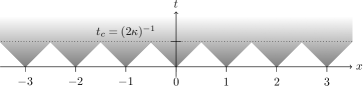
Figure 1: When $g(x)=\sum_{n\in\mathbb{N}}2^{-n}\left(|x-n|^{-1/2}+|x+n|^{-1/2}\right)$ and $\mu\equiv 0$, the random field solution $u(t,x)$ is only defined in the unshaded regions and in particular not for $t>t_{c}=(2\kappa)^{-1}$.

Example 3.5.

Let $g(x)=|x|^{-1/2}$ and $\mu\equiv 0$. Clearly, $g\not\in L_{loc}^{2}\left(\mathbb{R}\right)$. So Theorem 3.1 does not apply. In this case, the solution $u(t,x)$ is well defined outside of the triangle $\kappa\>t\geq|x|$. But because

$$J_{0}^{2}(t,x)=\frac{1}{4}\left(\frac{1}{|x+\kappa t|^{1/2}}+\frac{1}{|x-\kappa t|^{1/2}}\right)^{2},$$

and this function is not locally integrable over domains that intersect the characteristic lines $x=\pm\kappa t$ (see Assumption 2.4), the random field solution exists only in the two “triangles” $\kappa\>t\leq|x|$. Another example is shown in Figure 1.

3.2 Some lemmas and propositions for the existence theorem

Define the backward space-time cone:

$$\Lambda(t,x)=\left\{\left(s,y\right)\in\mathbb{R}_{+}\times\mathbb{R}:\;0\leq s\leq t,\;\;|y-x|\leq\kappa(t-s)\right\}$$

and the wave kernel function can be equivalently written as $G_{\kappa}\left(t-s,x-y\right)=\frac{1}{2}1_{\Lambda(t,x)}\left(s,y\right)$. The change of variables $u=\kappa s-y$, $w=\kappa s+y$ will play an important role: see Figure 2.

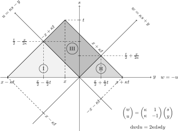
Figure 2: Change variables for the case where $|x|\leq\kappa t$.

For all $n\in\mathbb{N}^{*}$ and $(t,x)\in\mathbb{R}_{+}^{*}\times\mathbb{R}$, recall that $\mathcal{L}_{0}(t,x;\lambda)=\lambda^{2}G_{\kappa}^{2}(t,x)$ and $\mathcal{L}_{n}(t,x;\lambda)=(\mathcal{L}_{0}\star\dots\star\mathcal{L}_{0})(t,x)$, where there are $n+1$ convolutions of $\mathcal{L}_{0}(\cdot,\circ;\lambda)$.

Proposition 3.6.

For all $n\in\mathbb{N}$, and $(t,x)\in\mathbb{R}_{+}^{*}\times\mathbb{R}$,

$$\mathcal{L}_{n}(t,x)=\begin{cases}\frac{\lambda^{2n+2}\left((\kappa t)^{2}-x^{2}\right)^{n}}{2^{3n+2}(n!)^{2}\kappa^{n}}&\text{if $-\kappa t\leq x\leq\kappa t$,}\cr 0&\text{otherwise},\end{cases}$$ (3.13)

$$\mathcal{K}(t,x)=\sum_{n=0}^{\infty}\mathcal{L}_{n}(t,x),\;\text{and}$$ (3.14)

$$\left(\mathcal{K}\star\mathcal{L}_{0}\right)(t,x)=\mathcal{K}(t,x)-\mathcal{L}_{0}(t,x)\>.$$ (3.15)

Moreover, there are non-negative functions $B_{n}(t)$ such that for all $n\in\mathbb{N}$, the function $B_{n}(t)$ is nondecreasing in $t$ and $\mathcal{L}_{n}\leq\mathcal{L}_{0}(t,x)B_{n}(t)$ for all $(t,x)\in\mathbb{R}_{+}^{*}\times\mathbb{R}$, and

$$\sum_{n=1}^{\infty}\left(B_{n}(t)\right)^{1/m}<+\infty,\quad\text{for all $m\in\mathbb{N}^{*}$.}$$

Proof.

Formula (3.13) clearly holds for $n=0$. By induction, suppose that it is true for $n$. Now we evaluate $\mathcal{L}_{n+1}(t,x)$ from the definition and a change of variables (see Figure 2):

$$\mathcal{L}_{n+1}(t,x) =\left(\mathcal{L}_{0}\star\mathcal{L}_{n}\right)(t,x)=\frac{\lambda^{2n+4}}{2^{3n+4}(n!)^{2}\kappa^{n}}\>\frac{1}{2\kappa}\int_{0}^{x-\kappa t}\mathrm{d}u\>u^{n}\int_{0}^{x+\kappa t}\mathrm{d}w\>w^{n}$$

$$=\frac{\lambda^{2(n+1)+2}\left((\kappa t)^{2}-x^{2}\right)^{n+1}}{2^{3(n+1)+2}((n+1)!)^{2}\kappa^{n+1}}$$

for $-\kappa t\leq x\leq\kappa t$, and $\mathcal{L}_{n+1}(t,x)=0$ otherwise. This proves (3.13). The series in (3.14) converges to the modified Bessel function of order zero by (3.2). As a direct consequence, we have (3.15). Take $B_{n}(t)=\frac{\lambda^{2n}(\kappa t)^{2n}}{2^{3n}(n!)^{2}\kappa^{n}}$, which is non-negative and nondecreasing in $t$. Then clearly, $\mathcal{L}_{n}(t,x)\leq\mathcal{L}_{0}(t,x)B_{n}(t)$. To show the convergence, by the ratio test, for all $m\in\mathbb{N}^{*}$, we have that

$$\frac{\left(B_{n}(t)\right)^{1/m}}{\left(B_{n-1}(t)\right)^{1/m}}=\left(\frac{\lambda\sqrt{\kappa}\>t}{2\sqrt{2}}\right)^{\frac{2}{m}}\left(\frac{1}{n}\right)^{\frac{2}{m}}\rightarrow 0,$$

as $n\rightarrow\infty$. This completes the proof. ∎

Lemma 3.7.

The kernel function $\mathcal{K}(t,x)$ defined in (3.1) is strictly increasing in $t$ for $x\in\mathbb{R}$ fixed and decreasing in $|x|$ for $t>0$ fixed. Moreover, for all $\left(s,y\right)\in[0,t]\times\mathbb{R}$, we have that

$$\frac{\lambda^{2}}{2}G_{\kappa}\left(s,y\right)\leq\mathcal{K}\left(s,y\right)\leq\frac{\lambda^{2}}{2}I_{0}\left(|\lambda|\sqrt{\kappa/2}\>t\right)G_{\kappa}\left(s,y\right).$$

Proof.

The first part is true by (3.2). As for the inequalities, the upper bound follows from the first part. The lower bound is clear since $I_{0}(0)=1$ by (3.2). ∎

Lemma 3.8.

Recall the definition of $T_{k}(t,x)$ in (3.5). For all $t\in\mathbb{R}_{+}$, and $x,y\in\mathbb{R}$,

$$G_{\kappa}(t-s,x-z)G_{\kappa}\!\left(t-s,y-z\right)\!=\!\frac{1}{2}G_{\kappa}\left(\!T_{\kappa}\left(t,x-y\right)-s,\frac{x+y}{2}-z\!\right)\!,$$ (3.16)

$$\int_{\mathbb{R}}\mathrm{d}z\>G_{\kappa}(t,x-z)G_{\kappa}(t,y-z)=\frac{\kappa}{2}\>T_{\kappa}\left(t,x-y\right),\;\text{and}$$ (3.17)

$$\iint_{\mathbb{R}_{+}\times\mathbb{R}}\mathrm{d}s\mathrm{d}z\>G_{\kappa}(t-s,x-z)G_{\kappa}\left(t-s,y-z\right)=\frac{\kappa}{4}\>T^{2}_{\kappa}\left(t,x-y\right).$$ (3.18)

Proof.

Since $G_{\kappa}(t-s,x-y)=\frac{1}{2}1_{\left\{\Lambda(t,x)\right\}}\left(s,y\right)$, (3.16)–(3.18) are clear from Figure 3. ∎

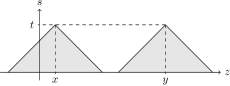
(a) the case where $|x-y|\geq 2\kappa t$

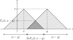
(b) the case where $|x-y|<2\kappa t$

Figure 3: The two lightly shaded regions denote the support of the functions $(s,z)\mapsto G_{\kappa}(t-s,x-z)$ and $(s,z)\mapsto G_{\kappa}\left(t-s,y-z\right)$ respectively.

Proposition 3.9.

The wave kernel function $G_{\kappa}(t,x)$ satisfies Assumption 2.5 with $\tau=1/2$, $\alpha=\kappa/2$ and all $\beta\in\;]0,1[$ and $C=1$.

Proof.

See Figure 4. The gray box is the set $B_{t,x,\beta,\tau,\alpha}$. Clearly, we need $\alpha/\kappa+\tau=1$. Therefore, we can choose $\tau=1/2$ and $\alpha=\kappa/2$. ∎

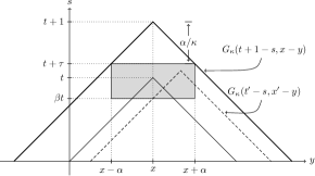
Figure 4: $G_{\kappa}(t,x)$ verifies Assumption 2.5.

For $g\in L_{loc}^{2}\left(\mathbb{R}\right)$ and $\mu\in\mathcal{M}\left(\mathbb{R}\right)$, define

$$\Psi_{g}(x)=\int_{-x}^{x}\mathrm{d}y\>g^{2}(y),\quad\text{and}\quad\Psi_{\mu}^{*}(x)=\left(|\mu|\left([-x,x]\right)\right)^{2}\;,\quad\text{for all $x\geq 0$.}$$ (3.19)

Clearly, these are nondecreasing functions of $x$.

Lemma 3.10.

If $g\in L_{loc}^{2}\left(\mathbb{R}\right)$ and $\mu\in\mathcal{M}\left(\mathbb{R}\right)$, then for all $v\in\mathbb{R}$ and $(t,x)\in\mathbb{R}_{+}\times\mathbb{R}$,

$$\left(\left[v^{2}+J_{0}^{2}\right]\star G_{\kappa}^{2}\right)(t,x)\leq\frac{\kappa t^{2}}{4}\left(v^{2}+3\Psi_{\mu}^{*}\left(|x|+\kappa t\right)\right)+\frac{3}{16}\>t\>\Psi_{g}\left(|x|+\kappa t\right)<+\infty.$$

Moreover, for all $v\in\mathbb{R}$ and all compact sets $K\subseteq\mathbb{R}_{+}\times\mathbb{R}$,

$$\sup_{(t,x)\in K}\left(\left[v^{2}+J_{0}^{2}\right]\star G_{\kappa}^{2}\right)(t,x)<+\infty.$$

Note that the conclusion of this lemma is stronger than Assumption 2.4 since $t$ can be zero here.

Proof.

Suppose $t>0$. Notice that $\left|(\mu*G_{\kappa}(s,\cdot))(y)\right|\leq|\mu|\left([y-\kappa s,y+\kappa s]\right)$, and so, recalling (1.7),

$$\left(\left[v^{2}+J_{0}^{2}\right]\star G_{\kappa}^{2}\right)(t,x) =\frac{1}{4}\left(v^{2}\>\iint_{\Lambda(t,x)}\mathrm{d}s\mathrm{d}y+\iint_{\Lambda(t,x)}\mathrm{d}s\mathrm{d}y\;J_{0}^{2}\left(s,y\right)\right)$$

$$\leq\frac{1}{4}\Bigg{(}v^{2}\kappa t^{2}+\frac{3}{4}\int_{0}^{t}\mathrm{d}s\int_{x-\kappa(t-s)}^{x+\kappa(t-s)}\mathrm{d}y\;\big{(}g^{2}(y+\kappa s)+g^{2}(y-\kappa s)$$

$$\hskip 40.0pt+4|\mu|^{2}\left([y-\kappa s,y+\kappa s]\right)\big{)}\Bigg{)}\>.$$

Clearly, for all $\left(s,y\right)\in\Lambda(t,x)$, by (3.19),

$$|\mu|^{2}\left([y-\kappa s,y+\kappa s]\right)\leq|\mu|^{2}\left([x-\kappa t,x+\kappa t]\right)\leq\Psi_{\mu}^{*}\left(|x|+\kappa t\right)\>.$$

The integral for $g^{2}$ can be easily evaluated by the change of variables in Figure 2:

$$\int_{0}^{t}\mathrm{d}s\int_{x-\kappa(t-s)}^{x+\kappa(t-s)}\left(g^{2}(y+\kappa s)+g^{2}(y-\kappa s)\right)\mathrm{d}y =\frac{1}{2\kappa}\iint_{I\cup II\cup III}\left(g^{2}(u)+g^{2}(w)\right)\mathrm{d}u\mathrm{d}w$$

$$\leq\frac{1}{2\kappa}\int_{x-\kappa t}^{x+\kappa t}\mathrm{d}w\int_{-x-\kappa t}^{-x+\kappa t}\mathrm{d}u\left(g^{2}(u)+g^{2}(w)\right)$$

$$\leq t\>\Psi_{g}(|x|+\kappa t)\>,$$

where $I$, $II$ and $III$ denote the three regions in Figure 2 and $\Psi_{g}$ is defined in (3.19). Therefore,

$$\left(\left[v^{2}+J_{0}^{2}\right]\star G_{\kappa}^{2}\right)(t,x)\leq\frac{1}{4}\left(\left(v^{2}+3\Psi_{\mu}^{*}\left(|x|+\kappa t\right)\right)\kappa t^{2}+\frac{3}{4}\;t\;\Psi_{g}\left(|x|+\kappa t\right)\right)<+\infty\>.$$

Finally, let $a=\sup\big{\{}|x|+\kappa t:(t,x)\in K\big{\}}$, which is finite because $K$ is a compact set. Then,

$$\sup_{(t,x)\in K}\left(\left[v^{2}+J_{0}^{2}\right]\star G_{\kappa}^{2}\right)(t,x)\leq\frac{\kappa a^{2}}{4}\left(v^{2}+3\Psi_{\mu}^{*}\left(a\right)\right)+\frac{3}{16}\>a\>\Psi_{g}\left(a\right)<+\infty\>,$$

which completes the proof of Lemma 3.10. ∎

Proof of Theorem 3.1.

To apply Theorem 2.13, we need to verify the assumptions (G) and (W) of Theorem 2.13 with $\theta(t,x)\equiv 1$. We begin with (G): (a) is satisfied by

$$\Theta_{\kappa}(t,x,x)=\iint_{[0,t]\times\mathbb{R}}\mathrm{d}s\mathrm{d}y\>G_{\kappa}^{2}\left(t-s,x-y\right)=\frac{\kappa t^{2}}{2}<+\infty$$

and Proposition 3.6; (b) is verified by Lemma 3.10. (W) is true due to Proposition 3.9. As for the two-point correlation function, (2.27) reduces to (3.12) because, by (3.16),

$$\int_{0}^{t}\mathrm{d}s\int_{\mathbb{R}}\mathrm{d}z\>f(s,z)G_{\kappa}(t-s,x-z)G_{\kappa}\left(t-s,y-z\right)=\frac{1}{2}\left(f\star G_{\kappa}\right)\left(T_{\kappa}\left(t,x-y\right),\frac{x+y}{2}\right).$$

This completes the proof of Theorem 3.1. ∎

3.3 Weak intermittency

Recall that $u(t,x)$ is said to be fully intermittent if the Lyapunov exponent of order $1$ vanishes and the lower Lyapunov exponent of order $2$ is strictly positive: $m_{1}=0$ and $\underline{m}_{2}>0$. The solution is called weakly intermittent if $\underline{m}_{2}>0$.

Theorem 3.11.

Suppose that $|\rho(u)|^{2}\leq\operatorname{\mathit{L}}_{\rho}^{2}(\operatorname{\overline{\varsigma}}^{2}+u^{2})$, $g(x)\equiv w$ and $\mu(\mathrm{d}x)=\widetilde{w}\mathrm{d}x$ with $w,\widetilde{w}\in\mathbb{R}$. Then we have the following two properties

1. For all even integers $p\geq 2$,

   $$\overline{m}_{p}\leq\begin{cases}\operatorname{\mathit{L}}_{\rho}\sqrt{2\kappa}\>p^{3/2}&\text{if $\operatorname{\overline{\varsigma}}\neq 0$ and $p>2$},\cr\operatorname{\mathit{L}}_{\rho}\sqrt{\kappa}\>p^{3/2}&\text{if $\operatorname{\overline{\varsigma}}=0$ and $p>2$},\cr\operatorname{\mathit{L}}_{\rho}\sqrt{\kappa/2}&\text{if $p=2$}.\end{cases}$$ (3.20)

2. If $|\rho(u)|^{2}\geq\operatorname{\mathit{l}}_{\rho}^{2}(\operatorname{\underline{\varsigma}}^{2}+u^{2})$ for some $\operatorname{\mathit{l}}_{\rho}\neq 0$, and if $|\operatorname{\underline{\varsigma}}|+|w|+|\widetilde{w}|\neq 0$ with $w\widetilde{w}\geq 0$, then $\underline{m}_{2}\geq|\operatorname{\mathit{l}}_{\rho}|\sqrt{\kappa/2}$ and so $u(t,x)$ is weakly intermittent.

3. If $|\rho(u)|^{2}=\lambda^{2}(\operatorname{\varsigma}^{2}+u^{2})$, with $\lambda\neq 0$, and if $|\operatorname{\underline{\varsigma}}|+|w|+|\widetilde{w}|\neq 0$, then $\underline{m}_{2}=\overline{m}_{2}=|\lambda|\sqrt{\kappa/2}$.

Proof.

Clearly, $J_{0}(t,x)=w+\kappa\widetilde{w}t$. (1) If $|\operatorname{\overline{\varsigma}}|+|w|+|\widetilde{w}|=0$, then $J_{0}(t,x)\equiv 0$ and $\rho(0)=0$, so $u(t,x)\equiv 0$ and the bound is trivially true. If $|\operatorname{\overline{\varsigma}}|+|w|+|\widetilde{w}|\neq 0$, then by (3.7), for all even integers $p\geq 2$,

$$\left|\left|u(t,x)\right|\right|_{p}^{2}\leq 2\left(w+\kappa\widetilde{w}t\right)^{2}+\left[\operatorname{\overline{\varsigma}}^{2}+2\left(w+\kappa\widetilde{w}t\right)^{2}\right]\widehat{\mathcal{H}}_{p}(t).$$

Hence, by (3.3), $\overline{m}_{p}\leq a_{p,\operatorname{\overline{\varsigma}}}z_{p}\operatorname{\mathit{L}}_{\rho}\sqrt{\kappa/2}\>p/2$. Then by (2.15) and the fact that $z_{2}=1$ and $z_{p}\leq 2\sqrt{p}$ for $p\geq 2$, we obtain (3.20).

(2) Note that the term $\operatorname{\overline{\varsigma}}^{2}+2\left(w+\kappa\widetilde{w}t\right)^{2}$ on the r.h.s. of the above inequality does not vanish since $|\operatorname{\overline{\varsigma}}|+|w|+|\widetilde{w}|\neq 0$. By (3.9) and Corollary 3.2,

$$\left|\left|u(t,x)\right|\right|_{2}^{2}\geq-\operatorname{\underline{\varsigma}}^{2}-\frac{4\kappa\widetilde{w}^{2}}{\operatorname{\mathit{l}}_{\rho}^{2}}+\left(w^{2}+\operatorname{\underline{\varsigma}}^{2}+\frac{4\kappa\widetilde{w}^{2}}{\operatorname{\mathit{l}}_{\rho}^{2}}\right)\cosh\left(|\operatorname{\mathit{l}}_{\rho}|\sqrt{\kappa/2}\>t\right).$$

Clearly, $|\operatorname{\underline{\varsigma}}|+|w|+|\widetilde{w}|\neq 0$ implies that $\underline{m}_{2}\geq|\operatorname{\mathit{l}}_{\rho}|\sqrt{\kappa/2}$.

Part (3) is a consequence of (1) and (2). This completes the proof of Theorem 3.11. ∎

Remark 3.12.

It would be interesting to obtain a lower bound of the form $\underline{m}_{p}\geq Cp^{3/2}$. Dalang and Mueller [23] derived the lower bound for the stochastic wave and heat equations in $\mathbb{R}_{+}\times\mathbb{R}^{3}$ in the case where $\rho(u)=\lambda u$ and the driving noise is spatially colored. An essential tool in their paper is a Feynman-Kac-type formula that they obtained (with Tribe) in [24].

3.4 Exponential growth indices

Recall the definition of $\underline{\lambda}_{p}(x)$ and $\overline{\lambda}_{p}(x)$ in (1.3) and (1.4). Define

$$\mathcal{M}_{G}^{\beta}\left(\mathbb{R}\right):=\left\{\mu\in\mathcal{M}\left(\mathbb{R}\right):\>\int_{\mathbb{R}}e^{\beta|x|}|\mu|(\mathrm{d}x)<+\infty\right\}\;,\quad\beta\geq 0.$$ (3.21)

We use subscript “$+$” to denote the subset of non-negative measures. For example, $\mathcal{M}_{+}\left(\mathbb{R}\right)$ is the set of non-negative Borel measures over $\mathbb{R}$ and $\mathcal{M}_{G,+}^{\beta}\left(\mathbb{R}\right)=\mathcal{M}_{G}^{\beta}\left(\mathbb{R}\right)\cap\mathcal{M}_{+}\left(\mathbb{R}\right)$.

Remark 3.13.

Since the kernel function $\mathcal{K}(t,x)$ has support in the same space-time cone as the fundamental solution $G_{\kappa}(t,x)$, it is clear that if the initial data have compact support, then the solution, including any high peaks related to intermittency, must propagate in the space-time cone with the same speed $\kappa$. Hence $\underline{\lambda}(p)\leq\overline{\lambda}(p)\leq\kappa$. Conus and Khoshnevisan showed in [18, Theorem 5.1] that with some other mild conditions on the compactly supported initial data, $\underline{\lambda}(p)=\overline{\lambda}(p)=\kappa$ for all $p\geq 2$.

Theorem 3.14.

We have the following:

1. Suppose that $|\rho(u)|\leq\operatorname{\mathit{L}}_{\rho}|u|$ with $\operatorname{\mathit{L}}_{\rho}\neq 0$ and the initial data satisfy the following two conditions:

   1. The initial position $g(x)$ is a Borel function such that $|g(x)|$ is bounded from above by some function $ce^{-\beta_{1}|x|}$ with $c>0$ and $\beta_{1}>0$ for almost all $x\in\mathbb{R}$;

   2. The initial velocity $\mu\in\mathcal{M}_{G}^{\beta_{2}}\left(\mathbb{R}\right)$ for some $\beta_{2}>0$.

   Then for all even integers $p\geq 2$,

   $$\overline{\lambda}(p)\leq\begin{cases}\displaystyle\kappa\left(1+\frac{a_{p,\operatorname{\overline{\varsigma}}}^{2}\>z_{p}^{2}\>\operatorname{\mathit{L}}_{\rho}^{2}}{8\kappa\>(\beta_{1}\wedge\beta_{2})^{2}}\right)^{1/2}&\text{if $p>2$},\\[10.00002pt] \displaystyle\kappa\left(1+\frac{\operatorname{\mathit{L}}_{\rho}^{2}}{8\kappa\>(\beta_{1}\wedge\beta_{2})^{2}}\right)^{1/2}&\text{if $p=2$}.\end{cases}$$

2. Suppose that $|\rho(u)|\geq\operatorname{\mathit{l}}_{\rho}|u|$ with $\operatorname{\mathit{l}}_{\rho}\neq 0$ and the initial data satisfy one of the following two conditions:

   1. The initial position $g(x)$ is a non-negative Borel function bounded from below by some function $c_{1}e^{-\beta_{1}^{\prime}|x|}$ with $c_{1}>0$ and $\beta_{1}^{\prime}>0$ for almost all $x\in\mathbb{R}$;

   2. The initial velocity $\mu(\mathrm{d}x)$ has a density $\mu(x)$ that is a non-negative Borel function bounded from below by some function $c_{2}e^{-\beta_{2}^{\prime}|x|}$ with $c_{2}>0$ and $\beta_{2}^{\prime}>0$ for almost all $x\in\mathbb{R}$.

   Then

   $$\underline{\lambda}(p)\geq\kappa\left(1+\frac{\operatorname{\mathit{l}}_{\rho}^{2}}{8\kappa\left(\beta_{1}^{\prime}\wedge\beta_{2}^{\prime}\right)^{2}}\right)^{1/2},\quad\text{for all even integers $p\geq 2$.}$$

In particular, we have the following two special cases:

1. For the hyperbolic Anderson model $\rho(u)=\lambda u$ with $\lambda\neq 0$, if the initial velocity $\mu$ satisfies all Conditions (a), (b), (a’) and (b’) with $\beta:=\beta_{1}\wedge\beta_{2}=\beta_{1}^{\prime}\wedge\beta_{2}^{\prime}$, then

   $$\underline{\lambda}(2)=\overline{\lambda}(2)=\kappa\left(1+\frac{\lambda^{2}}{8\kappa\beta^{2}}\right)^{1/2}.$$

2. If $\operatorname{\mathit{l}}_{\rho}|u|\leq|\rho(u)|\leq\operatorname{\mathit{L}}_{\rho}|u|$ with $\operatorname{\mathit{l}}_{\rho}\neq 0$ and $\operatorname{\mathit{L}}_{\rho}\neq 0$, and both $g(x)$ and $\mu(x)$ are non-negative Borel functions with compact support, then

   $$\overline{\lambda}(p)=\underline{\lambda}(p)=\kappa,\quad\text{for all even integers $p\geq 2$.}$$

Proof.

The statements of (1) and (2) are a consequence of Propositions 3.17 and 3.20 below. More precisely, let $J_{0,1}(t,x)$ (resp. $J_{0,2}(t,x)$) be the homogeneous solutions obtained with the initial data $g$ and $0$ (resp. $0$ and $\mu$). Clearly, $J_{0}(t,x)=J_{0,1}(t,x)+J_{0,2}(t,x)$. For the upper bounds, we use the fact that $J_{0}^{2}(t,x)\leq 2J_{0,1}^{2}(t,x)+2J_{0,2}^{2}(t,x)$. By (3.7), we simply choose the larger of the upper bounds between Proposition 3.17 (1) and Proposition 3.20 (1). As for the lower bounds, because both $g$ and $\mu$ are nonnegative, $J_{0}^{2}(t,x)\geq J_{0,1}^{2}(t,x)+J_{0,2}^{2}(t,x)$. Hence, by (3.9), we only need to take the larger of the lower bounds between Proposition 3.17 (2) and Proposition 3.20 (2). Part (3) is a direct consequence of (1) and (2). When the initial data have compact support, both (1) and (2) hold for all $\beta_{i}>0$ with $i=1,2$. Then letting these $\beta_{i}$’s tend to $+\infty$ proves (4). ∎

Note that for Conclusion (3), clearly, $\beta_{i}^{\prime}\geq\beta_{i}$, $i=1,2$. Hence, the condition $\beta_{1}\wedge\beta_{2}=\beta_{1}^{\prime}\wedge\beta_{2}^{\prime}$ has only two possible cases: $\beta_{1}^{\prime}=\beta_{1}\leq\beta_{2}\leq\beta_{2}^{\prime}$ and $\beta_{2}^{\prime}=\beta_{2}\leq\beta_{1}\leq\beta_{1}^{\prime}$.

Remark 3.15.

The behaviour of growth indices of the solution to the stochastic wave equation (1.8) depends on the growth rate of the nonlinearity of $\rho$, and also on the rate of decay at $\pm\infty$ of the initial data. In particular, the initial data significantly affects the behavior of the solution for all time. However, when the initial data are compactly supported, the growth rate of the non-linearity $\rho$ plays no role.

3.5 Two propositions for the exponential growth indices

The following asymptotic formula for $I_{0}(x)$ (see, [38, (10.30.4)]) will be useful

$$I_{0}(x)\sim\frac{e^{x}}{\sqrt{2\pi x}},\quad\text{as $x\rightarrow\infty$.}$$ (3.22)

3.5.1 Contributions of the initial position

First consider the case where $\mu\equiv 0$. Recall that $H(t)$ is the Heaviside function.

Lemma 3.16.

Let $f(t,x)=\frac{1}{2}\left(e^{-\beta|x-\kappa t|}+e^{-\beta|x+\kappa t|}\right)H(t)$. Then we have the following bounds:

1. Set $\sigma:=\sqrt{\beta^{2}+\frac{\lambda^{2}}{2\kappa}}$. For $\beta>0$, $t\geq 0$ and $|x|\geq\kappa t$,

   $$\left(f\star\mathcal{K}\right)(t,x)\leq\frac{\lambda^{2}\>t}{2(\sigma-\beta)}e^{-\beta|x|+\kappa\sigma t}\>.$$

2. For $(t,x)\in\mathbb{R}_{+}^{*}\times\mathbb{R}$, $\beta>0$ and $a,b\in\;]0,1[$,

   $$\left(f\star\mathcal{K}\right)(t,x)\geq\begin{cases}\frac{1}{2}e^{-\beta\kappa t}\cosh(\beta|x|)\left(I_{0}\left(\sqrt{\frac{\lambda^{2}(\kappa^{2}t^{2}-x^{2})}{2\kappa}}\right)-1\right)&\text{if $|x|\leq\kappa t$,}\cr\frac{\lambda^{2}e^{-\beta|x|}}{2(1-a^{2})\beta^{2}\kappa}I_{0}\left(\sqrt{\frac{\lambda^{2}(1-a^{2})}{2\kappa}}\>b\>\kappa t\right)g(t\;;a,b,\beta,\kappa)&\text{if $|x|\geq\kappa t$\>,}\end{cases}$$

   where the function $g\left(t\;;a,b,\beta,\kappa\right)$ is equal to

   $$a\cosh\left(ab\beta\kappa t\right)\cosh\left((1-b)\beta\kappa t\right)-a\cosh\left(a\beta\kappa t\right)+\sinh\left((1-b)\beta\kappa t\right)\sinh\left(ab\beta\kappa t\right).$$

Proof.

(1) Because $f(t,\circ)$ and $\mathcal{K}(t,\circ)$ are even functions, it suffices to consider the case $x\leq-\kappa t$. In this case, $y\leq-\kappa s$ implies that $f(s,y)=\frac{1}{2}\left(e^{\beta(y-\kappa s)}+e^{\beta(y+\kappa s)}\right)H(s)$. Hence, by (3.4),

$$\left(f\star\mathcal{K}\right)(t,x) \leq\frac{\lambda^{2}}{4}\int_{0}^{t}\mathrm{d}s\int_{x-\kappa(t-s)}^{x+\kappa(t-s)}\mathrm{d}y\;\frac{1}{2}\left(e^{\beta(y-\kappa s)}+e^{\beta(y+\kappa s)}\right)\exp\left(\sqrt{\frac{\lambda^{2}[\kappa^{2}(t-s)^{2}-(x-y)^{2}]}{2\kappa}}\right)$$

$$=\frac{\lambda^{2}}{8}\int_{0}^{t}\mathrm{d}s\>\left(e^{\beta(x-\kappa(t-s))}+e^{\beta(x+\kappa(t-s))}\right)\int_{-\kappa s}^{\kappa s}\mathrm{d}y\;\exp\left(-\beta y+\sqrt{\frac{\lambda^{2}[\kappa^{2}s^{2}-y^{2}]}{2\kappa}}\right).$$

The function $\psi(y):=-\beta y+\left[\lambda^{2}(\kappa^{2}s^{2}-y^{2})/(2\kappa)\right]^{1/2}$ achieves its maximum at $y=-\sigma^{-1}\beta\kappa s\in[-\kappa s,\kappa s]$, and $\max_{|y|\leq\kappa s}\psi(y)=\sigma\kappa s$, so

$$\left(f\star\mathcal{K}\right)(t,x) \leq\frac{\lambda^{2}\kappa\>t}{4}\int_{0}^{t}\mathrm{d}s\>\left(e^{\beta(x-\kappa t)+\kappa(\sigma+\beta)s}+e^{\beta(x+\kappa t)+\kappa(\sigma-\beta)s}\right)$$

$$\leq\frac{\lambda^{2}t}{4(\sigma-\beta)}\left(e^{\beta(x-\kappa t)+\kappa(\sigma+\beta)t}+e^{\beta(x+\kappa t)+\kappa(\sigma-\beta)t}\right)=\frac{\lambda^{2}t}{2(\sigma-\beta)}e^{\beta x+\kappa\sigma t}\;.$$

(2) We consider two cases. Case I: $|x|\leq\kappa t$. As shown in Figure 2, we decompose the space-time convolution into three parts $S_{i}$ corresponding to the three integration regions $D_{i}$, $i=1,2,3$:

$$\left(f\star G_{\kappa}\right)(t,x)=\sum_{i=1}^{3}S_{i}=\sum_{i=1}^{3}\frac{1}{2}\iint_{D_{i}}\mathrm{d}s\mathrm{d}y\>f(s,y).$$

Clearly, $\left(f\star\mathcal{K}\right)(t,x)\geq S_{3}$. Because

$$f\left(s,y\right)\geq\frac{1}{2}\left(e^{-\beta(\kappa t-x)}+e^{-\beta(\kappa t+x)}\right),\quad\text{for all $(s,y)\in D_{3}$},$$

we see that

$$S_{3}\geq\frac{2}{\lambda^{2}}e^{-\beta\kappa t}\cosh\left(\beta x\right)\left(\mathcal{L}_{0}\star\mathcal{K}\right)(t,x).$$

Then apply (3.15).

Case II: $|x|\geq\kappa t$. Similar to the proof of part (1), one can assume that $x\leq-\kappa t$. Then

$$\left(f\star\mathcal{K}\right)(t,x)=\frac{\lambda^{2}}{8}\int_{0}^{t}\mathrm{d}s\int_{-\kappa s}^{\kappa s}\mathrm{d}y\>I_{0}\left(\sqrt{\frac{\lambda^{2}(\kappa^{2}s^{2}-y^{2})}{2\kappa}}\right)\left(e^{\beta(x-y-\kappa(t-s))}+e^{\beta(x-y+\kappa(t-s))}\right).$$

Fix $a,b\in\;]0,1[\>$. Then

$$\left(f\star\mathcal{K}\right)(t,x)\geq \;\frac{\lambda^{2}}{4}\int_{bt}^{t}\mathrm{d}s\int_{-a\kappa s}^{a\kappa s}\mathrm{d}y\>I_{0}\left(\sqrt{\frac{\lambda^{2}(\kappa^{2}s^{2}-y^{2})}{2\kappa}}\right)e^{\beta(x-y)}\cosh(\beta\kappa(t-s))$$

$$\geq \;\frac{\lambda^{2}e^{\beta x}}{4}I_{0}\left(\sqrt{\frac{\lambda^{2}(1-a^{2})}{2\kappa}}\>b\>\kappa t\right)\int_{bt}^{t}\mathrm{d}s\int_{-a\kappa s}^{a\kappa s}\mathrm{d}y\;\cosh(\beta\kappa(t-s))e^{-\beta y}\>.$$

Since

$$\int_{bt}^{t}\mathrm{d}s\int_{-a\kappa s}^{a\kappa s}\mathrm{d}y\>\cosh(\beta\kappa(t-s))e^{-\beta y}=\frac{2}{\beta}\int_{bt}^{t}\mathrm{d}s\>\cosh(\beta\kappa(t-s))\sinh(a\beta\kappa s),$$

part (2) is proved by an application of the integral in Lemma A.3. ∎

Proposition 3.17.

Suppose that $\mu\equiv 0$. Fix $\beta>0$. Then:

1. Suppose $|\rho(u)|\leq\operatorname{\mathit{L}}_{\rho}|u|$ with $\operatorname{\mathit{L}}_{\rho}\neq 0$ and let $g(x)$ be a measurable function such that for some constant $C>0$, $|g(x)|\leq Ce^{-\beta|x|}$ for almost all $x\in\mathbb{R}$. Then

   $$\overline{\lambda}(p)\leq\begin{cases}\displaystyle\kappa\left(1+\frac{a_{p,\operatorname{\overline{\varsigma}}}^{2}\>z_{p}^{2}\>\operatorname{\mathit{L}}_{\rho}^{2}}{8\kappa\beta^{2}}\right)^{1/2}&\text{if $p>2$ is an even integer},\\[10.00002pt] \displaystyle\kappa\left(1+\frac{\operatorname{\mathit{L}}_{\rho}^{2}}{8\kappa\beta^{2}}\right)^{1/2}&\text{if $p=2$}\>.\end{cases}$$ (3.23)

2. Suppose $|\rho(u)|\geq\operatorname{\mathit{l}}_{\rho}|u|$ with $\operatorname{\mathit{l}}_{\rho}\neq 0$ and let $g(x)$ be a measurable function such that for some constant $c>0$, $|g(x)|\geq c\>e^{-\beta|x|}$ for almost all $x\in\mathbb{R}$. Then

   $$\underline{\lambda}(p)\geq\kappa\left(1+\frac{\operatorname{\mathit{l}}_{\rho}^{2}}{8\kappa\beta^{2}}\right)^{1/2},\quad\text{for all even integers $p\geq 2$.}$$ (3.24)

In particular, if $g(x)$ satisfies both Conditions (1) and (2), and $\rho(u)=\lambda u$ with $\lambda\neq 0$, then

$$\underline{\lambda}(2)=\overline{\lambda}(2)=\kappa\left(1+\frac{\lambda^{2}}{8\kappa\beta^{2}}\right)^{1/2}.$$ (3.25)

Proof.

(1) Let $J_{0}(t,x)=\frac{1}{2}\left(g(x-\kappa t)+g(x+\kappa t)\right)H(t)$. By the assumptions on $g(x)$,

$$\left|J_{0}(t,x)\right|^{2}\leq\frac{C^{2}}{2}\left(e^{-2\beta|x-\kappa t|}+e^{-2\beta|x+\kappa t|}\right)H(t),\quad\text{for almost all $(t,x)\in\mathbb{R}_{+}\times\mathbb{R}$.}$$

We first consider the case $p>2$. By the moment formula (3.7) and Lemma 3.16 (1), for $|x|\geq\kappa t$,

$$\left|\left|u(t,x)\right|\right|_{p}^{2}\leq 2J_{0}^{2}(t,x)+C^{\prime}t\exp\left(-2\beta|x|+\kappa\sigma t\right),$$

for some constant $C^{\prime}>0$, where $\sigma:=\left[4\beta^{2}+(2\kappa)^{-1}a_{p,\operatorname{\overline{\varsigma}}}^{2}\>z_{p}^{2}\operatorname{\mathit{L}}_{\rho}^{2}\>\right]^{1/2}$. We only need to consider the case where $\alpha>\kappa$; see Remark 3.13. Because the supremum over $|x|\geq\alpha t$ of the right-hand side is attained at $|x|=\alpha t$,

$$\lim_{t\rightarrow\infty}\frac{1}{t}\sup_{|x|\geq\alpha t}\log\left|\left|u(t,x)\right|\right|_{p}^{p}\leq-2\alpha\beta+\kappa\sigma,\quad\text{for $\alpha>\kappa$.}$$

Solve the inequality $-2\alpha\beta+\kappa\sigma<0$ to get $\overline{\lambda}(p)\leq\kappa\frac{\sigma}{2\beta}$, which is the formula in (3.23) for $p>2$. For the case $p=2$, we simply replace $z_{p}$ and $a_{p,\operatorname{\overline{\varsigma}}}$ by $1$ (see (2.15)).

(2) Note that $\underline{\lambda}(p)\geq\underline{\lambda}(2)$, because $\left|\left|u\right|\right|_{p}\geq\left|\left|u\right|\right|_{2}$ for $p\geq 2$, we only need to consider $p=2$. Assume first that $\rho(u)=\lambda u$. Since $|g(x)|\geq c\>e^{-\beta|x|}$ a.e.,

$$J_{0}^{2}(t,x)\geq\frac{c^{2}}{4}\left(e^{-2\beta|x-\kappa t|}+e^{-2\beta|x+\kappa t|}\right).$$

If $|x|\leq\kappa t$, by (3.9), Lemma 3.7 and Lemma 3.16,

$$\left|\left|u(t,x)\right|\right|_{2}^{2}\geq\left(J_{0}^{2}\star\mathcal{K}\right)(t,x)\geq\frac{c^{2}}{4}e^{-2\beta\kappa t}\cosh(2\beta|x|)\left(I_{0}\left(\sqrt{\frac{\lambda^{2}(\kappa^{2}t^{2}-x^{2})}{2\kappa}}\right)-1\right).$$

Hence, for $0\leq\alpha<\kappa$, by (3.22),

$$\lim_{t\rightarrow+\infty}\frac{1}{t}\sup_{|x|\geq\alpha t}\log\left|\left|u(t,x)\right|\right|_{2}^{2}\geq-2\beta\kappa+2\beta\alpha+|\lambda|\sqrt{\frac{\kappa^{2}-\alpha^{2}}{2\kappa}}\>.$$

Then

$$h(\alpha):=-2\beta\kappa+2\beta\alpha+\frac{|\lambda|}{\sqrt{2\kappa}}\sqrt{\kappa^{2}-\alpha^{2}}\geq 0\quad\Leftrightarrow\quad\kappa\;\frac{8\kappa\beta^{2}-\lambda^{2}}{8\kappa\beta^{2}+\lambda^{2}}\leq\alpha\leq\kappa.$$

As $\alpha$ tends to $\kappa$ from the left side, $h(\alpha)$ remains positive. Therefore, $\underline{\lambda}(2)\geq\kappa$.

If $x\leq-\kappa t$, again, by Lemma 3.16,

$$\left|\left|u(t,x)\right|\right|_{2}^{2}\geq\frac{c^{2}\lambda^{2}e^{-2\beta|x|}}{4(1-a^{2})(2\beta)^{2}\kappa}I_{0}\left(\sqrt{\frac{\lambda^{2}(1-a^{2})}{2\kappa}}b\kappa t\right)g(t\;;a,b,2\beta,\kappa),\quad\text{for all $a,b\in\;]0,1[$.}$$

For large $t$, replace both $\cosh(Ct)$ and $\sinh(Ct)$ by $\exp(Ct)/2$, with $C\geq 0$, to see that

$$g(t\;;a,b,2\beta,\kappa)\geq C^{\prime}\exp\left(2(1+(a-1)b)t\beta\kappa\right),$$

for some constant $C^{\prime}>0$. Hence, for $\alpha>\kappa$, by (3.22),

$$\lim_{t\rightarrow\infty}\frac{1}{t}\sup_{|x|\geq\alpha t}\log\left|\left|u(t,x)\right|\right|_{2}^{2}\geq\sqrt{\frac{\lambda^{2}(1-a^{2})}{2\kappa}}b\kappa-2\beta\alpha+2(1-(1-a)b)\beta\kappa\;.$$

Solve the inequality

$$h(\alpha):=\sqrt{\frac{\lambda^{2}(1-a^{2})}{2\kappa}}b\kappa-2\beta\alpha+2(1-(1-a)b)\beta\kappa>0$$

to get

$$\alpha<\left(\sqrt{\frac{\lambda^{2}(1-a^{2})}{2\kappa}}\frac{b}{2\beta}+1-(1-a)b\right)\kappa.$$

Since $a\in\;]0,1[$ is arbitrary, we can choose

$$a:=\mathop{\arg\max}_{a\in\;]0,1[}\left(\sqrt{\frac{\lambda^{2}(1-a^{2})}{2\kappa}}\frac{b}{2\beta}+1-(1-a)b\right)=\left(1+\frac{\lambda^{2}}{8\kappa\beta^{2}}\right)^{-1/2}.$$

In this case, the critical growth rate is $\alpha=b\kappa\left[1+\lambda^{2}/(8\kappa\beta^{2})\right]^{1/2}+(1-b)\kappa$. Finally, since $b$ can be arbitrarily close to $1$, we have that $\underline{\lambda}(2)\geq\kappa\left[1+\lambda^{2}/(8\kappa\beta^{2})\right]^{1/2}$, and for the general case $|\rho(u)|\geq\operatorname{\mathit{l}}_{\rho}|u|$, we have that $\underline{\lambda}(p)\geq\underline{\lambda}(2)\geq\kappa\left[1+\operatorname{\mathit{l}}_{\rho}^{2}/(8\kappa\beta^{2})\right]^{1/2}$. This completes the proof of Proposition 3.17. ∎

3.5.2 Contributions of the initial velocity

Now, let us consider the case where $g(x)\equiv 0$. We shall first study the case where $\mu(\mathrm{d}x)=e^{-\beta|x|}\mathrm{d}x$ with $\beta>0$. In this case, $J_{0}(t,x)$ is given by the following lemma.

Lemma 3.18.

Suppose that $\mu(\mathrm{d}x)=e^{-\beta|x|}\mathrm{d}x$ with $\beta>0$. For all $(t,x)\in\mathbb{R}_{+}\times\mathbb{R}$ and $z>0$,

$$\left(\mu*1_{\left\{|\cdot|\leq z\right\}}\right)(x)=\begin{cases}2\beta^{-1}e^{-\beta|x|}\sinh(\beta z)&|x|\geq z,\cr 2\beta^{-1}\left(1-e^{-\beta z}\cosh(\beta x)\right)&|x|\leq z.\end{cases}$$

In particular, we have that $J_{0}(t,x)=\begin{cases}\beta^{-1}e^{-\beta|x|}\sinh(\beta\kappa t)&|x|\geq\kappa t,\cr\beta^{-1}\left(1-e^{-\beta\kappa t}\cosh(\beta x)\right)&|x|\leq\kappa t.\end{cases}$

The proof is straightforward, and is left to the reader (see also [10, Lemma 4.4.5]).

Lemma 3.19.

Suppose that $\mu\in\mathcal{M}_{G}^{\beta}\left(\mathbb{R}\right)$ with $\beta>0$. Set $h(t,x)=\left(\mu*G_{\kappa}(t,\cdot)\right)(x)$ and $\sigma=\left[\beta^{2}+(2\kappa)^{-1}\lambda^{2}\right]^{1/2}$. Then for all $t\geq 0$ and $x\in\mathbb{R}$,

$$\left|h(t,x)\right|\leq C\exp\left(\beta\kappa t-\beta|x|\right),\quad\text{with $C=1/2\int_{\mathbb{R}}|\mu|(\mathrm{d}x)\>e^{\beta|x|}$}\>,$$

and

$$\left(|h|\star\mathcal{K}\right)(t,x)\leq\frac{\lambda^{2}t}{2(\sigma-\beta)}e^{-\beta|x|+\sigma\kappa t}.$$

Proof.

Considering the first inequality, observe that

$$e^{\beta|x|}\left|\left(\mu*G_{\kappa}(t,\cdot)\right)(x)\right| \leq\frac{1}{2}\int_{x-\kappa t}^{x+\kappa t}|\mu|(\mathrm{d}y)\>e^{\beta|x|}\leq\frac{1}{2}\int_{x-\kappa t}^{x+\kappa t}|\mu|(\mathrm{d}y)\>e^{\beta|x-y|}e^{\beta|y|}$$

$$\leq\frac{1}{2}e^{\beta\kappa t}\int_{x-\kappa t}^{x+\kappa t}|\mu|(\mathrm{d}y)\>e^{\beta|y|}\leq\frac{1}{2}e^{\beta\kappa t}\int_{\mathbb{R}}|\mu|(\mathrm{d}y)\>e^{\beta|y|}.$$

For the second inequality, set $f(t,x)=e^{\beta\kappa t-\beta|x|}$. Then by (3.4),

$$\left(f\star\mathcal{K}\right)(t,x) =\frac{\lambda^{2}}{4}\int_{0}^{t}\mathrm{d}s\>e^{\beta\kappa(t-s)}\int_{-\kappa s}^{\kappa s}\mathrm{d}y\>\exp\left(-\beta|x-y|+\sqrt{\frac{\lambda^{2}\left(\kappa^{2}s^{2}-y^{2}\right)}{2\kappa}}\right)$$

$$\leq\frac{\lambda^{2}}{4}\int_{0}^{t}\mathrm{d}s\>e^{\beta\kappa(t-s)}\int_{-\kappa s}^{\kappa s}\mathrm{d}y\>\exp\left(-\beta|x|+\beta|y|+\sqrt{\frac{\lambda^{2}\left(\kappa^{2}s^{2}-y^{2}\right)}{2\kappa}}\right)$$

$$\leq\frac{\lambda^{2}}{2}e^{-\beta|x|}\int_{0}^{t}\mathrm{d}s\>e^{\beta\kappa(t-s)}\int_{0}^{\kappa s}\mathrm{d}y\>\exp\left(\beta y+\sqrt{\frac{\lambda^{2}\left(\kappa^{2}s^{2}-y^{2}\right)}{2\kappa}}\right).$$

The function $\psi(y):=\beta y+\left[\lambda^{2}\left(\kappa^{2}s^{2}-y^{2}\right)/(2\kappa)\right]^{1/2}$ achieves its maximum at $y=\sigma^{-1}\beta\kappa s\in[0,\kappa s]$, and $\max_{y\in[0,\kappa s]}\psi(y)=\sigma\kappa s$, so

$$\left(f\star\mathcal{K}\right) \leq\frac{\lambda^{2}\kappa t}{2}e^{-\beta|x|}\int_{0}^{t}\mathrm{d}s\>e^{\beta\kappa(t-s)+\sigma\kappa s}\leq\frac{\lambda^{2}t}{2(\sigma-\beta)}e^{-\beta|x|+\sigma\kappa t}\>.$$

This completes the proof. ∎

Proposition 3.20.

Suppose that $g\equiv 0$. Fix $\beta>0$.

1. If $|\rho(u)|\leq\operatorname{\mathit{L}}_{\rho}|u|$ with $\operatorname{\mathit{L}}_{\rho}\neq 0$ and $\mu\in\mathcal{M}_{G}^{\beta}\left(\mathbb{R}\right)$, then $\overline{\lambda}(p)$ satisfies (3.23).

2. Suppose that $|\rho(u)|\geq\operatorname{\mathit{l}}_{\rho}|u|$ with $\operatorname{\mathit{l}}_{\rho}\neq 0$ and $\mu(\mathrm{d}x)=f(x)\mathrm{d}x$. If for some constant $c>0$, $f(x)\geq ce^{-\beta|x|}$ for all almost all $x\in\mathbb{R}$, then $\underline{\lambda}(p)$ satisfies (3.24).

In particular, if $\mu$ satisfies both Conditions (1) and (2), and $\rho(u)=\lambda u$ with $\lambda\neq 0$, then (3.25) holds.

Proof.

(1) Let $p>2$ be an even integer. Let $h(t,x)$ be the function defined in Lemma 3.19. Notice that the first bound in Lemma 3.19 is satisfied by $h^{2}(t,x)$ provided $\beta$ is replaced by $2\beta$. By (3.7) and Lemma 3.19, we see that for some constant $C^{\prime}>0$,

$$\left|\left|u(t,x)\right|\right|_{p}^{2}\leq 2h^{2}(t,x)+C^{\prime}t\exp\left(-2\beta|x|+\kappa\sigma t\right),$$

where $\sigma=\left[4\beta^{2}+a_{p,\operatorname{\overline{\varsigma}}}^{2}\>z_{p}^{2}\>\operatorname{\mathit{L}}_{\rho}^{2}/(2\kappa)\right]^{1/2}$. Then it is clear that

$$\lim_{t\rightarrow\infty}\frac{1}{t}\sup_{|x|\geq\alpha t}\log\left|\left|u(t,x)\right|\right|_{p}^{p}\leq-2\beta\alpha+\kappa\sigma.$$

Solve the inequality $-2\beta\alpha+\kappa\sigma>0$ to get $\overline{\lambda}(p)\leq\kappa\frac{\sigma}{2\beta}$. For the case $p=2$, simply replace $z_{p}$ and $a_{p,\operatorname{\overline{\varsigma}}}$ by $1$.

(2) Suppose that $f(x)\geq e^{-\beta|x|}$ for almost all $x\in\mathbb{R}$ (i.e., set $c=1$). By (3.9) and (3.11), we may only consider the case where $\rho(u)=\lambda u$. Denote $J_{0}(t,x)=(e^{-\beta|\cdot|}*G_{\kappa}(t,\cdot))(x)$. We first consider the case where $|x|\leq\kappa t$. As shown in Figure 2, split the integral that defines $\left(J_{0}^{2}\star\mathcal{K}\right)(t,x)$ over the three regions I, II, and III, so that

$$\left|\left|u(t,x)\right|\right|_{2}^{2}\geq\left(J_{0}^{2}\star\mathcal{K}\right)(t,x)=S_{1}+S_{2}+S_{3}\geq S_{3}.$$

For arbitrary $a,b\in\;]0,1[$, we see that

$$S_{3} \geq\frac{\lambda^{2}}{4}\int_{bt}^{t}\mathrm{d}s\int_{-a\kappa s}^{a\kappa s}\mathrm{d}y\;J_{0}^{2}\left(t-s,x-y\right)I_{0}\left(\sqrt{\frac{\lambda^{2}\left((\kappa s)^{2}-y^{2}\right)}{2\kappa}}\right)$$

$$\geq\frac{\lambda^{2}}{4}\int_{bt}^{t}\mathrm{d}s\;I_{0}\left(\sqrt{\frac{\lambda^{2}\left(1-a^{2}\right)}{2\kappa}}\;\kappa s\right)\int_{-a\kappa s}^{a\kappa s}\mathrm{d}y\;J_{0}^{2}\left(t-s,x-y\right)$$

$$\geq\frac{\lambda^{2}}{4}I_{0}\left(\sqrt{\frac{\lambda^{2}\left(1-a^{2}\right)}{2\kappa}}\;\kappa bt\right)\int_{bt}^{t}\mathrm{d}s\int_{-ab\kappa t}^{ab\kappa t}\mathrm{d}y\;J_{0}^{2}\left(t-s,x-y\right).$$

Clearly, for $\left(s,y\right)$ in Region III of Figure 2, $|x-y|\leq\kappa(t-s)$ and so by Lemma 3.18,

$$J_{0}\left(t-s,x-y\right)=\left(1-e^{-\beta\kappa(t-s)}\cosh\left(\beta(x-y)\right)\right)/\beta.$$

Using the inequalities $(a+b)^{2}\geq\frac{a^{2}}{2}-b^{2}$ and $\cosh^{2}(x)=\frac{1}{2}\left(\cosh(2x)+1\right)\geq\frac{1}{2}\cosh(2x)$,

$$J_{0}^{2}\left(t-s,x-y\right)\geq\frac{1}{4\beta^{2}}\>e^{-2\beta\kappa(t-s)}\cosh(2\beta(x-y))-\frac{1}{\beta^{2}}\>.$$

Hence,

$$\int_{bt}^{t}\mathrm{d}s\int_{-ab\kappa t}^{ab\kappa t}\mathrm{d}y\>J_{0}^{2}\left(t-s,x-y\right)\geq\frac{\left(1-e^{-2(1-b)\beta\kappa t}\right)\cosh(2\beta x)\sinh(2ab\beta\kappa t)}{8\beta^{4}\kappa}-\frac{2a(1-b)b\kappa t^{2}}{\beta^{2}}\>.$$

Therefore, by (3.22),

$$\lim_{t\rightarrow+\infty}\frac{1}{t}\sup_{|x|\geq\alpha t}\log\left|\left|u(t,x)\right|\right|_{2}^{2}\geq 2\beta\alpha+2ab\beta\kappa+b|\lambda|\sqrt{\kappa/2}\>\sqrt{1-a^{2}}\;>0,$$ (3.26)

for $\alpha\leq\kappa$ and all $a,b\in\;]0,1[\>$, which implies that $\underline{\lambda}(2)\geq\kappa$. As for the case where $|x|\geq\kappa t$, for all $a,b\in\;]0,1[$, by Lemma 3.18,

$$\left|\left|u(t,x)\right|\right|_{2}^{2} \geq\left(J^{2}_{0}\star\mathcal{K}\right)(t,x)$$

$$=\frac{\lambda^{2}}{16\beta^{2}}\int_{0}^{t}\mathrm{d}s\sinh^{2}(\beta\kappa(t-s))\int_{-\kappa s}^{\kappa s}\mathrm{d}y\>e^{-2\beta|x-y|}I_{0}\left(\sqrt{\frac{\lambda^{2}(\kappa^{2}s^{2}-y^{2})}{2\kappa}}\right)$$

$$\geq\frac{\lambda^{2}e^{-2\beta|x|+2a\kappa bt\beta}}{32\beta^{3}}\left(\frac{\sinh(2(1-b)\beta\kappa t)}{4\beta\kappa}-\frac{1}{2}(1-b)t\right)I_{0}\left(\sqrt{\frac{\lambda^{2}(1-a^{2})}{2\kappa}}b\kappa t\right).$$

Therefore, for $\alpha>\kappa$, we obtain the same inequality as (3.26). The rest argument is exactly the same as the proof of part (2) of Proposition 3.17. This completes the proof of Proposition 3.20. ∎

4 Hölder continuity in the stochastic wave equation

Theorem 4.1.

Suppose that $\rho$ is Lipschitz continuous. If $g\in L_{loc}^{2\gamma}\left(\mathbb{R}\right)$, $\gamma\geq 1$ and $\mu\in\mathcal{M}\left(\mathbb{R}\right)$, then for all compact sets $K\in\mathbb{R}_{+}\times\mathbb{R}$ and all $p\geq 1$, there is a constant $C_{K,p}$ such that for all $(t,x)$, $(t^{\prime},x^{\prime})\in K$,

$$\left|\left|I(t,x)-I(t^{\prime},x^{\prime})\right|\right|_{p}\leq C_{K,p}\left(|t-t^{\prime}|^{1/(2\gamma^{\prime})}+|x-x^{\prime}|^{1/(2\gamma^{\prime})}\right),$$

where $\frac{1}{\gamma}+\frac{1}{\gamma^{\prime}}=1$. Hence,

$$I(t,x)\in C_{\frac{1}{2\gamma^{\prime}}-,\frac{1}{2\gamma^{\prime}}-}\left(\mathbb{R}_{+}\times\mathbb{R}\right)\;\text{a.s. }$$

In addition, for all compact sets $K\in\mathbb{R}_{+}\times\mathbb{R}$ and $0\leq\alpha<1/(2\gamma^{\prime})-2/p$,

$$\mathbb{E}\left[\left(\mathop{\sup_{(t,x),\;(s,y)\in K}}_{(t,x)\neq(s,y)}\frac{|I(t,x)-I(s,y)|}{\left[|t-s|+|x-y|\right]^{\alpha}}\right)^{p}\;\right]<+\infty.$$

In particular, if $g$ is locally bounded ($\gamma=+\infty$), then $I(t,x)\in C_{\frac{1}{2}-,\frac{1}{2}-}\left(\mathbb{R}_{+}\times\mathbb{R}\right)$ a.s.

Proof.

We only need to verify that Assumption 2.14 holds for $K_{n}=[0,n]\times[-n,n]$. This is the case thanks to Propositions 4.5 – 4.7 below. More precisely, let $J_{0,1}(t,x)$ and $J_{0,2}(t,x)$ be the homogeneous solutions contributed respectively by $g$ and $\mu$. Clearly, when both $g$ and $\mu$ are nonvanishing, $J_{0}(t,x)=J_{0,1}(t,x)+J_{0,2}(t,x)$. Because $J_{0}^{2}(t,x)\leq 2J_{0,1}^{2}(t,x)+2J_{0,2}^{2}(t,x)$, we can consider $J_{0,1}(t,x)$ and $J_{0,2}(t,x)$ separately when verifying Assumption 2.14. In particular, Proposition 4.5 shows that the contribution of $J_{0,2}(t,x)$ satisfies Assumption 2.14, and Propositions 4.6 and 4.7 guarantee that the contribution of $J_{0,1}(t,x)$ satisfies Assumption 2.14. ∎

Proposition 4.2.

Suppose that $\left|\rho(u)\right|^{2}=\lambda^{2}\left(\operatorname{\varsigma}^{2}+u^{2}\right)$. If $g(x)=|x|^{-a}$ with $a\in\left[0,1/2\right[$ and $\mu\equiv 0$, then in the neighborhood of the two characteristic lines $|x|=\kappa t$, the function $I(t,x)$ mapping from $\mathbb{R}_{+}\times\mathbb{R}$ into $L^{p}(\Omega)$, $p\geq 2$, cannot be $\rho$-Hölder continuous either in space or in time with $\rho>\frac{1-2a}{2}$.

This proposition is proved in Section 4.2.

Remark 4.3 (Optimal $L^{p}(\Omega)$-Hölder continuity).

Clearly, $|x|^{-a}\in L_{loc}^{2\gamma}\left(\mathbb{R}\right)$ if and only if $2\gamma a<1$, i.e., $\gamma<(2a)^{-1}$. Hence, $\gamma^{\prime}$, the dual of $\gamma$, is strictly bigger than $(1-2a)^{-1}$. Therefore, according to Theorem 4.1, for all $p\geq 2$, the function $I:\mathbb{R}_{+}\times\mathbb{R}\mapsto L^{p}(\Omega)$ is jointly $\eta$-Hölder continuous with $\eta=(1-2a)/2$. For example, if $a=1/4$ (see Example 3.4), then $I$ is jointly $1/4$-Hölder continuous in $L^{p}(\Omega)$. Proposition 4.2 then shows that $I(t,x)$ cannot be jointly $\eta$-Hölder continuous with $\eta>1/4$. Hence, the estimates on the joint $L^{p}(\Omega)$-Hölder continuity are optimal. Singularities in the initial conditions affect the regularity of deviations from the homogeneous solution.

4.1 Three propositions for the Hölder continuity

In this part, we will prove Propositions 4.5 – 4.7, which together verify Assumption 2.14 (and hence the Hölder continuity).

Proposition 4.4.

For $T>0$, we have that

$$\int_{\mathbb{R}_{+}}\mathrm{d}s\int_{\mathbb{R}}\mathrm{d}y\left(G_{\kappa}\left(t-s,x-y\right)-G_{\kappa}(t^{\prime}-s,x^{\prime}-y)\right)^{2}\leq C_{T}\left(\left|x^{\prime}-x\right|+\left|t^{\prime}-t\right|\right),$$

for all $(t,x)$ and $\left(t^{\prime},x^{\prime}\right)\in\>]0,T]\times\mathbb{R}$, with $C_{T}:=\left(\kappa\vee 1\right)T/2$.

The proof of this proposition is elementary.

Proposition 4.5.

Denote $K_{n}^{*}:=[0,n]\times[-n-\kappa n,n+\kappa n]$. Suppose that

$$\sup_{(t,x)\in K_{n}^{*}}J_{0}^{2}(t,x)<+\infty,\quad\text{for all $n>0$.}$$ (4.1)

Then Assumption 2.14 holds under the settings: $\theta(t,x)\equiv 1$, $d=1$, $\gamma_{0}=\gamma_{1}=1$, and $K_{n}=[0,n]\times[-n,n]$. Condition (4.1) (and hence Assumption (2.14)) holds in particular when $g\equiv 0$ and $\mu$ is a locally finite Borel measure:

$$\sup_{(t,x)\in K_{n}^{*}}J_{0}^{2}(t,x)\leq 1/4\;\Psi_{\mu}^{*}\left(n+2\kappa n\right)<+\infty.$$

Proof.

Fix $v\geq 0$, $n>1$ and choose arbitrary $(t,x)$ and $(t^{\prime},x^{\prime})\in K_{n}=[0,n]\times[-n,n]$ (note that the time variable can be zero). Because the support of the function $\left(s,y\right)\mapsto G_{\kappa}\left(t-s,x-y\right)-G_{\kappa}\left(t^{\prime}-s,x^{\prime}-y\right)$ is included in the compact set $K_{n}^{*}$, by Proposition 4.4, the l.h.s. of (2.28) is bounded by,

$$C_{n}\iint_{\mathbb{R}_{+}\times\mathbb{R}}\mathrm{d}s\mathrm{d}y\>\left(G_{\kappa}\left(t-s,x-y\right)-G_{\kappa}\left(t^{\prime}-s,x^{\prime}-y\right)\right)^{2}\leq C_{n}\frac{n\left(\kappa\vee 1\right)}{2}\left(\left|x-x^{\prime}\right|+\left|t-t^{\prime}\right|\right),$$

where $C_{n}=\sup_{\left(s,y\right)\in K_{n}^{*}}\left(v^{2}+2J_{0}^{2}\left(s,y\right)\right)$. As for (2.29), using the same constant $C_{n}$, the l.h.s. of (2.29) is bounded by

$$C_{n}\iint_{\mathbb{R}_{+}\times\mathbb{R}}\mathrm{d}s\mathrm{d}y\left[\iint_{\mathbb{R}_{+}\times\mathbb{R}}\mathrm{d}u\mathrm{d}z\>G_{\kappa}^{2}(s-u,y-z)\right]\left(G_{\kappa}\left(t-s,x-y\right)-G_{\kappa}\left(t^{\prime}-s,x^{\prime}-y\right)\right)^{2}\\ \leq\frac{C_{n}\kappa n^{2}}{4}\iint_{\mathbb{R}_{+}\times\mathbb{R}}\mathrm{d}s\mathrm{d}y\>(G_{\kappa}\left(t-s,x-y\right)-G_{\kappa}\left(t^{\prime}-s,x^{\prime}-y\right))^{2}.$$

Then apply Proposition 4.4 as before. ∎

Proposition 4.6.

Suppose $\mu\equiv 0$ and $g\in L_{loc}^{2}\left(\mathbb{R}\right)$. Then (2.29) holds with $\theta(t,x)\equiv 1$, $d=1$, $\gamma_{0}=\gamma_{1}=1$, and $K_{n}=[0,n]\times[-n,n]$.

Proof.

Split (2.29) into two parts by linearity: one term is contributed by $v^{2}$ and the other by $2J_{0}^{2}$. Proposition 4.5 shows that the first term satisfies Assumption 2.14. Hence, we only need to consider the second term. Let $K_{n}^{*}=[0,n]\times\left[-(1+\kappa)n,(1+\kappa)n\right]$. By a change of variables (see Figure 2), for all $(t,x)\in K_{n}^{*}$,

$$\left(J_{0}^{2}\star G_{\kappa}^{2}\right)(t,x)=\frac{1}{16}\frac{1}{2\kappa}\iint_{I\cup II\cup III}\mathrm{d}u\mathrm{d}w\>\left(g(w)+g(u)\right)^{2}\leq\frac{(1+\kappa)n}{4\kappa}\Psi_{g}(n+n\kappa),$$

where $I$, $II$ and $III$ denote the three domains shown in Figure 2. Therefore, this proposition is proved by applying Proposition 4.5. ∎

Proposition 4.7.

Suppose $\mu\equiv 0$, $g\in L_{loc}^{2\gamma}\left(\mathbb{R}\right)$ with $\gamma\geq 1$, and $1/\gamma+1/\gamma^{\prime}=1$. Then (2.28) holds with $\theta(t,x)\equiv 1$, $d=1$, and $\gamma_{0}=\gamma_{1}=1/\gamma^{\prime}$.

Proof.

Equivalently, we shall show that (2.30)–(2.32) hold under the same settings. As explained in the proof of Proposition 4.6, we can assume that $v=0$ in (2.30)–(2.32). Fix $n>0$, $(t,x)$ and $(t^{\prime},x^{\prime})\in K_{n}=[0,n]\times[-n,n]$ with $t\leq t^{\prime}$. We first prove (2.30). Because the support of the function $G_{\kappa}-G_{\kappa}$ is in $K_{n}^{*}=[0,n]\times[-(1+\kappa)n,(1+\kappa)n]$, by Hölder’s inequality,

$$I :=\int_{0}^{t}\mathrm{d}s\int_{\mathbb{R}}\mathrm{d}y\>J_{0}^{2}\left(s,y\right)\left(G_{\kappa}\left(t-s,x-y\right)-G_{\kappa}(t^{\prime}-s,x-y)\right)^{2}$$

$$\leq\int_{0}^{t}\mathrm{d}s\left(\int_{-(1+\kappa)n}^{(1+\kappa)n}\mathrm{d}y\>J_{0}^{2\gamma}\left(s,y\right)\right)^{1/\gamma}\left(\int_{\mathbb{R}}\mathrm{d}y\left|G_{\kappa}\left(t-s,x-y\right)-G_{\kappa}(t^{\prime}-s,x-y)\right|^{2\gamma^{\prime}}\right)^{1/\gamma^{\prime}}.$$

By convexity of $x\mapsto|x|^{2\gamma}$,

$$\int_{-(1+\kappa)n}^{(1+\kappa)n}\mathrm{d}y\>J_{0}^{2\gamma}\left(s,y\right)\leq\frac{1}{2}\int_{-(1+\kappa)n}^{(1+\kappa)n}\mathrm{d}y\>\left(g^{2\gamma}(y+\kappa s)+g^{2\gamma}(y-\kappa s)\right)\leq\Psi_{g^{\gamma}}(n+2\kappa n).$$

Hence,

$$I\leq\Psi_{g^{\gamma}}^{\frac{1}{\gamma}}(n+2\kappa n)\int_{0}^{t}\mathrm{d}s\left(\int_{\mathbb{R}}\mathrm{d}y\left|G_{\kappa}\left(t-s,x-y\right)-G_{\kappa}(t^{\prime}-s,x-y)\right|^{2\gamma^{\prime}}\right)^{1/\gamma^{\prime}},$$

where

$$\int_{\mathbb{R}}\mathrm{d}y\>\left|G_{\kappa}\left(t-s,x-y\right)-G_{\kappa}(t^{\prime}-s,x-y)\right|^{2\gamma^{\prime}}=2^{-2\gamma^{\prime}}\kappa n\left|t^{\prime}-t\right|.$$

Therefore,

$$I\leq\frac{\kappa^{1/\gamma^{\prime}}n^{1+1/\gamma^{\prime}}}{4}\Psi_{g^{\gamma}}^{\frac{1}{\gamma}}(n+2\kappa n)\left|t^{\prime}-t\right|^{1/\gamma^{\prime}},$$

which proves (2.30).

Now let us consider (2.31). As above, we can assume that $v=0$, so we set

$$I :=\int_{0}^{t}\mathrm{d}s\int_{\mathbb{R}}\mathrm{d}y\>J_{0}^{2}\left(s,y\right)(G_{\kappa}\left(t-s,x-y\right)-G_{\kappa}(t-s,x^{\prime}-y))^{2}$$

$$\leq\Psi_{g^{\gamma}}^{\frac{1}{\gamma}}(n+2\kappa n)\int_{0}^{t}\mathrm{d}s\left(\int_{\mathbb{R}}\mathrm{d}y\>\left|G_{\kappa}\left(t-s,x-y\right)-G_{\kappa}(t-s,x^{\prime}-y)\right|^{2\gamma^{\prime}}\right)^{1/\gamma^{\prime}},$$

where (see Figure 3),

$$\int_{\mathbb{R}}\mathrm{d}y\>\left|G_{\kappa}\left(t-s,x-y\right)-G_{\kappa}(t-s,x^{\prime}-y)\right|^{2\gamma^{\prime}}\\ =2^{1-2\gamma^{\prime}}\left|x^{\prime}-x\right|\>1_{\left\{\left|x^{\prime}-x\right|\leq 2\kappa(t-s)\right\}}+2^{1-2\gamma^{\prime}}\kappa(t-s)\>1_{\left\{\left|x^{\prime}-x\right|>2\kappa(t-s)\right\}}\leq 2^{1-2\gamma^{\prime}}\left|x^{\prime}-x\right|.$$

Therefore,

$$I\leq 2^{-2+1/\gamma^{\prime}}n\>\Psi_{g^{\gamma}}^{\frac{1}{\gamma}}(n+2\kappa n)\>\left|x^{\prime}-x\right|^{1/\gamma^{\prime}},$$

which proves (2.31).

Now let us consider (2.32). By the same arguments as above, we only consider

$$I :=\int_{t}^{t^{\prime}}\mathrm{d}s\int_{\mathbb{R}}\mathrm{d}y\>J_{0}^{2}\left(s,y\right)G_{\kappa}^{2}(t^{\prime}-s,x^{\prime}-y)$$

$$\>\leq\Psi_{g^{\gamma}}^{\frac{1}{\gamma}}(n+2\kappa n)\int_{t}^{t^{\prime}}\mathrm{d}s\left(\int_{\mathbb{R}}\mathrm{d}y\>G_{\kappa}^{2\gamma^{\prime}}(t^{\prime}-s,x^{\prime}-y)\right)^{1/\gamma^{\prime}},$$

where

$$\int_{\mathbb{R}}\mathrm{d}y\>G_{\kappa}^{2\gamma^{\prime}}(t^{\prime}-s,x^{\prime}-y)=2^{-2\gamma^{\prime}}2\kappa(t^{\prime}-s)\leq 2^{-2\gamma^{\prime}}2\kappa n.$$

Therefore,

$$I\leq 2^{-2+1/\gamma^{\prime}}(n\kappa)^{1/\gamma^{\prime}}\Psi_{g^{\gamma}}^{\frac{1}{\gamma}}(n+2\kappa n)\left|t^{\prime}-t\right|.$$

Finally, (2.32) follows from the bound $\left|t^{\prime}-t\right|\leq n^{1/\gamma}\left|t^{\prime}-t\right|^{1/\gamma^{\prime}}$. ∎

4.2 Optimality of the Hölder exponents (proof of Proposition 4.2)

Lemma 4.8.

If $g(x)=|x|^{-a}$ with $a\in\left[0,1/2\right[$ and $\mu\equiv 0$, then

$$\left(J_{0}^{2}\star G_{\kappa}^{2}\right)(t,x)=\begin{cases}\frac{a^{2}-4a+2}{32\kappa(1-2a)(1-a)^{2}}\left|\kappa t-x\right|^{2(1-a)},&\text{if $x<-\kappa t$,}\cr\frac{1}{32\kappa(1-a)^{2}}\left[\left(\kappa t-x\right)^{1-a}+\left(\kappa t+x\right)^{1-a}\right]^{2}&\cr\quad+\frac{t}{16(1-2a)}\left[\left(\kappa t-x\right)^{1-2a}+\left(\kappa t+x\right)^{1-2a}\right],&\text{if $|x|\leq\kappa t$,}\cr\frac{a^{2}-4a+2}{32\kappa(1-2a)(1-a)^{2}}\left|\kappa t+x\right|^{2(1-a)},&\text{if $x>\kappa t$,}\end{cases}$$

where $J_{0}(t,x)=\left(g\left(x-\kappa t\right)+g\left(x+\kappa t\right)\right)/2$.

Proof.

First assume that $|x|\leq\kappa t$. Then

$$\left(J_{0}^{2}\star G_{\kappa}^{2}\right)(t,x)=\frac{1}{16}\int_{0}^{t}\mathrm{d}s\int_{x-\kappa(t-s)}^{x+\kappa(t-s)}\mathrm{d}y\>(g(y-\kappa s)+g(y+\kappa s))^{2}=\frac{1}{16}\left(S_{1}+S_{2}+S_{3}\right),$$

where $S_{1}$, $S_{2}$ and $S_{3}$ correspond to the integrations in the regions I, II and III shown in Figure 2. To evaluate these three integrals, by change the variables (see Figure 2),

$$S_{1}=\frac{1}{2\kappa}\int_{x-\kappa t}^{0}\mathrm{d}w\int_{-w}^{-x+\kappa t}\mathrm{d}u\left(\left|u\right|^{-a}+\left|w\right|^{-a}\right)^{2}=\frac{a^{2}-4a+2}{2\kappa(1-2a)(1-a)^{2}}\left(\kappa t-x\right)^{2(1-a)},$$

$$S_{2}=\frac{1}{2\kappa}\int_{0}^{x+\kappa t}\mathrm{d}w\int_{-w}^{0}\mathrm{d}u\left(\left|u\right|^{-a}+\left|w\right|^{-a}\right)^{2}=\frac{a^{2}-4a+2}{2\kappa(1-2a)(1-a)^{2}}\left(\kappa t+x\right)^{2(1-a)},$$

$$S_{3}=\frac{1}{\kappa(1-a)^{2}}\left(\kappa^{2}t^{2}-x^{2}\right)^{1-a}+\frac{1}{2\kappa(1-2a)}\left(\left(\kappa t-x\right)^{1-2a}\left(\kappa t+x\right)+\left(\kappa t+x\right)^{1-2a}\left(\kappa t-x\right)\right).$$

Use the fact that

$$\frac{a^{2}-4a+2}{2\kappa(1-2a)(1-a)^{2}}=\frac{(1-2a)+(1-a)^{2}}{2\kappa(1-2a)(1-a)^{2}}=\frac{1}{2\kappa(1-a)^{2}}+\frac{1}{2\kappa(1-2a)}$$

to sum up these $S_{i}$. The other two cases, $x<-\kappa t$ and $x>\kappa t$, can be calculated similarly to $S_{1}$ and $S_{2}$ respectively. ∎

Proof of Proposition 4.2.

Let $I(t,x)$ be the stochastic integral part of random field solution, i.e., $u(t,x)=J_{0}(t,x)+I(t,x)$. For $(t,x)$ and $(t^{\prime},x^{\prime})\in\mathbb{R}_{+}\times\mathbb{R}$, because

$$\operatorname{\varsigma}^{2}+\left|\left|u\left(s,y\right)\right|\right|_{2}^{2}\geq J_{0}^{2}\left(s,y\right),\quad\text{and}\quad\left|\left|I(t,x)-I(t^{\prime},x^{\prime})\right|\right|_{p}^{2}\geq\left|\left|I(t,x)-I(t^{\prime},x^{\prime})\right|\right|_{2}^{2}$$

for $p\geq 2$, we see that

$$\left|\left|I(t,x)-I(t^{\prime},x^{\prime})\right|\right|_{p}^{2}\\ \geq\lambda^{2}\iint_{\mathbb{R}_{+}\times\mathbb{R}}\mathrm{d}s\mathrm{d}y\>\left(G_{\kappa}\left(t-s,x-y\right)-G_{\kappa}(t^{\prime}-s,x^{\prime}-y)\right)^{2}J_{0}^{2}\left(s,y\right).\quad$$ (4.2)

Spatial increments. Fix $t=t^{\prime}>0$, $x$ and $x^{\prime}\in\mathbb{R}$. Denote $T=T_{\kappa}(t,x-x^{\prime})$. By (3.16), the lower bound in (4.2) reduces to

$$\lambda^{2}\iint_{\mathbb{R}_{+}\times\mathbb{R}}\mathrm{d}s\mathrm{d}y\>J_{0}^{2}\left(s,y\right)(G_{\kappa}^{2}\left(t-s,x-y\right)-2G_{\kappa}^{2}\left(T-s,\frac{x+x^{\prime}}{2}-y\right)+G_{\kappa}^{2}(t-s,x^{\prime}-y)),$$

which is denoted by $\lambda^{2}L(t,x,x^{\prime})$. Then

$$L(t,x,x^{\prime})=\left(J_{0}^{2}\star G_{\kappa}^{2}\right)(t,x)+\left(J_{0}^{2}\star G_{\kappa}^{2}\right)(t,x^{\prime})-2\left(J_{0}^{2}\star G_{\kappa}^{2}\right)\left(T,\frac{x+x^{\prime}}{2}\right).$$

Let $x=\kappa t$ and $x^{\prime}<x$ be such that $|x^{\prime}-x|\leq 2\kappa t$. Hence, $T_{\kappa}(t,x-x^{\prime})=t-(x-x^{\prime})/(2\kappa)$. Then apply Lemma 4.8 to see that

$$L(t,\kappa t,x^{\prime})=\frac{1}{32\kappa(1-a)^{2}}L_{1}(t,x^{\prime})+\frac{t}{16(1-2a)}L_{2}(t,x^{\prime}),$$

with

$$L_{1}(t,x^{\prime}) =(2\kappa t)^{2(1-a)}+\left[\left(\kappa t-x^{\prime}\right)^{1-a}+\left(\kappa t+x^{\prime}\right)^{1-a}\right]^{2}-2\left(\kappa t+x^{\prime}\right)^{2(1-a)},$$

$$L_{2}(t,x^{\prime}) =(2\kappa t)^{1-2a}+(\kappa t-x^{\prime})^{1-2a}-(\kappa t+x^{\prime})^{1-2a}.$$

Let $h=\kappa t-x^{\prime}$. Then

$$L_{1}(t,x^{\prime}) =(2\kappa t)^{2(1-a)}+\left[h^{1-a}+(2\kappa t-h)^{1-a}\right]^{2}-2\left(2\kappa t-h\right)^{2(1-a)}\geq h^{2(1-a)},$$

$$L_{2}(t,x^{\prime}) =(2\kappa t)^{1-2a}+h^{1-2a}-\left(2\kappa t-h\right)^{1-2a}\geq h^{1-2a}.$$

Since $1-2a\in\>\left]0,1\right]$ and $2(1-a)\in\;\left]1,2\right]$, by discarding $L_{1}(t,x^{\prime})$, we have that

$$\left|\left|I(t,\kappa t)-I(t,\kappa t-h)\right|\right|_{p}^{2}=\lambda^{2}L(t,\kappa t,x^{\prime})\geq\frac{\lambda^{2}t}{16(1-2a)}h^{1-2a}.$$

Time increments. Now fix $x=x^{\prime}\in\mathbb{R}$. By symmetry, we assume that $x>0$ . For $t^{\prime}\geq t\geq 0$, (4.2) implies that

$$\left|\left|I(t,x)-I(t^{\prime},x)\right|\right|_{p}^{2}\geq\lambda^{2}\left(\left(J_{0}^{2}\star G_{\kappa}^{2}\right)(t^{\prime},x)-\left(J_{0}^{2}\star G_{\kappa}^{2}\right)(t,x)\right),$$

because $G_{\kappa}(t,x)G_{\kappa}(t^{\prime},x)=G_{\kappa}^{2}(t,x)$. Take $t=x/\kappa$ and $h=t^{\prime}-t=t^{\prime}-x/\kappa$. Similarly to the previous case,

$$\left(J_{0}^{2}\star G_{\kappa}^{2}\right)\left(\frac{x}{\kappa},x\right)=\frac{1}{32\kappa(1-a)^{2}}\left(2x\right)^{2(1-a)}+\frac{x}{16\kappa(1-2a)}\left(2x\right)^{1-2a},$$

and $\left(J_{0}^{2}\star G_{\kappa}^{2}\right)\left(t^{\prime},x\right)$ is equal to

$$\frac{1}{32\kappa(1-a)^{2}}\left[\left(\kappa h\right)^{1-a}+\left(\kappa h+2x\right)^{1-a}\right]^{2}+\frac{x}{16\kappa(1-2a)}\left[\left(\kappa h\right)^{1-2a}+\left(\kappa h+2x\right)^{1-2a}\right].$$

Hence, by symmetry, for all $x\in\mathbb{R}$, and $h=t^{\prime}-|x|/\kappa>0$,

$$\left|\left|I\left(\frac{|x|}{\kappa},x\right)-I(t^{\prime},x)\right|\right|_{p}^{2}\geq\frac{\lambda^{2}|x|}{16\kappa^{2a}(1-2a)}h^{1-2a}.$$

Therefore, Proposition 4.2 is proved. ∎

Appendix A Some technical lemmas

Lemma A.1.

For $a\neq 0$ and $t\geq 0$, $\int_{0}^{t}\mathrm{d}s\>\cosh(as)(t-s)=a^{-2}\left(\cosh(at)-1\right)$, $\int_{0}^{t}\mathrm{d}s\>\sinh(as)(t-s)=a^{-2}\left(\sinh(at)-at\right)$, and $\int_{0}^{t}\mathrm{d}s\>\sinh(as)(t-s)^{2}=a^{-3}\left(2\cosh(at)-a^{2}t^{2}-2\right)$.

Lemma A.2.

For $t\geq 0$ and $x\in\mathbb{R}$, we have that $\int_{\mathbb{R}}\mathrm{d}x\>\mathcal{K}(t,x)=|\lambda|\>(\kappa/2)^{1/2}\sinh\left(|\lambda|\>(\kappa/2)^{1/2}t\right)$ and $\left(1\star\mathcal{K}\right)(t,x)=\cosh\left(|\lambda|\>(\kappa/2)^{1/2}t\right)-1$.

Proof.

By a change of variable,

$$\int_{\mathbb{R}}\mathrm{d}x\>\mathcal{K}(t,x)=2\int_{0}^{|\lambda|\sqrt{\kappa/2}\>t}\mathrm{d}y\>\frac{\lambda^{2}}{4}\frac{\sqrt{2\kappa}}{|\lambda|}\frac{y}{\sqrt{\kappa t^{2}\lambda^{2}/2-y^{2}}}I_{0}(y).$$

Then the first statement follows from [28, (6) on p. 365] with $\nu=0$, $\sigma=1/2$ and $a=|\lambda|\>(\kappa/2)^{1/2}t$. The second statement is a simple application of the first. ∎

Lemma A.3.

Suppose that $a\neq c$, $t>0$ and $b\in[0,1]$. Then

$$\int_{bt}^{t}\mathrm{d}s\>\cosh\left(a(t-s)\right)\sinh\left(cs\right)\\ =\left(a^{2}-c^{2}\right)^{-1}\Big{(}c\cosh(bct)\cosh\left(a(1-b)t\right)-c\cosh(ct)+a\sinh(bct)\sinh\left(a(1-b)t\right)\Big{)}.$$

Proof.

Use the formula $\cosh(x)\sinh(y)=\frac{1}{2}\left(\sinh(x+y)+\sinh(-x+y)\right)$. ∎

For the following two lemmas, let $G_{\nu}(t,x)$, $\nu>0$, be the heat kernel function (see (2.37)).

Lemma A.4.

For all $t$, $s>0$ and $x$, $y\in\mathbb{R}$, we have that $G_{\nu}^{2}(t,x)=\frac{1}{\sqrt{4\pi\nu t}}G_{\nu/2}(t,x)$ and $G_{\nu}(t,x)G_{\nu}\left(s,y\right)=G_{\nu}\left(\frac{ts}{t+s},\frac{sx+ty}{t+s}\right)G_{\nu}\left(t+s,x-y\right)$.

Lemma A.5 (Lemma 4.4 of [11]).

For all $x$, $z_{1}$ $z_{2}\in\mathbb{R}$ and $t,s>0$, denote $\bar{z}=\frac{z_{1}+z_{2}}{2}$, $\Delta z=z_{1}-z_{2}$. Then $G_{1}\left(t,x-\bar{z}\right)G_{1}\left(s,\Delta z\right)\leq\frac{(4t)\vee s}{\sqrt{ts}}G_{1}\!\left((4t)\vee s,x-z_{1}\right)G_{1}\!\left((4t)\vee s,x-z_{2}\right)$, where $a\vee b:=\max(a,b)$.

References

- [1] R. Balan and D. Conus. Intermittency for the wave and heat equations with fractional noise in time. Preprint at arXiv::1311.0021, 2013.
- [2] L. Bertini and N. Cancrini. The stochastic heat equation: Feynman-Kac formula and intermittence. J. Statist. Phys., 78(5-6):1377–1401, 1995.
- [3] P. Billingsley. Probability and measure ( ed.). John Wiley & Sons Inc., New York, 1995.
- [4] Z. Brzeźniak and M. Ondreját. Strong solutions to stochastic wave equations with values in Riemannian manifolds. J. Funct. Anal., 253(2):449–481, 2007.
- [5] Z. Brzeźniak and M. Ondreját. Weak solutions to stochastic wave equations with values in Riemannian manifolds. Comm. Partial Differential Equations, 36(9):1624–1653, 2011.
- [6] R. Cairoli and J. B. Walsh. Stochastic integrals in the plane. Acta Math., 134:111–183, 1975.
- [7] R. A. Carmona and S. A. Molchanov. Parabolic Anderson problem and intermittency. Mem. Amer. Math. Soc., 108(518), 1994.
- [8] R. A. Carmona and D. Nualart. Random nonlinear wave equations: propagation of singularities. Ann. Probab., 16(2):730–751, 1988.
- [9] R. Carmona and D. Nualart. Random nonlinear wave equations: smoothness of the solutions. Probab. Theory Related Fields, 79(4):469–508, 1988.
- [10] L. Chen. Moments, intermittency, and growth indices for nonlinear stochastic PDE’s with rough initial conditions. PhD thesis, No. 5712, École Polytechnique Fédérale de Lausanne, 2013.
- [11] L. Chen and R. C. Dalang. Moments and growth indices for the nonlinear stochastic heat equation with rough initial conditions. Preprint at arXiv:1307.0600, 2013.
- [12] L. Chen and R. C. Dalang. Hölder-continuity for the nonlinear stochastic heat equation with rough initial conditions. Preprint at arXiv::1310.6421, 2013.
- [13] P.-L. Chow. Stochastic wave equations with polynomial nonlinearity. Ann. Appl. Probab., 12(1):361–381, 2002.
- [14] K. L. Chung and R. J. Williams. Introduction to stochastic integration ( ed.). Birkhäuser Boston Inc., Boston, MA, 1990.
- [15] D. Conus and R. C. Dalang. The non-linear stochastic wave equation in high dimensions. Electron. J. Probab., 13:no. 22, 629–670, 2008.
- [16] D. Conus, M. Joseph, D. Khoshnevisan, and S.-Y. Shiu. Initial measures for the stochastic heat equation. Ann. Inst. Henri Poincaré Probab. Stat., to appear, 2013.
- [17] D. Conus, M. Joseph, D. Khoshnevisan, and S.-Y. Shiu. Intermittency and chaos for a stochastic non-linear wave equation in dimension 1. Preprint at arXiv:112.1909, 2011.
- [18] D. Conus and D. Khoshnevisan. On the existence and position of the farthest peaks of a family of stochastic heat and wave equations. Probab. Theory Related Fields, 152(3-4):681–701, 2012.
- [19] R. Dalang, D. Khoshnevisan, C. Mueller, D. Nualart, and Y. Xiao. A minicourse on stochastic partial differential equations. Springer-Verlag, Berlin, 2009.
- [20] R. C. Dalang. The stochastic wave equation. Chapter 2 in [19].
- [21] R. C. Dalang. Extending the martingale measure stochastic integral with applications to spatially homogeneous s.p.d.e.’s. Electron. J. Probab., 4:no. 6, 29 pp. (electronic), 1999.
- [22] R. C. Dalang and N. E. Frangos. The stochastic wave equation in two spatial dimensions. Ann. Probab., 26(1):187–212, 1998.
- [23] R. C. Dalang and C. Mueller. Intermittency properties in a hyperbolic Anderson problem. Ann. Inst. Henri Poincaré Probab. Stat., 45(4):1150–1164, 2009.
- [24] R. C. Dalang, C. Mueller, and R. Tribe. A Feynman-Kac-type formula for the deterministic and stochastic wave equations and other P.D.E.’s. Trans. Amer. Math. Soc., 360(9):4681–4703, 2008.
- [25] R. C. Dalang and L. Quer-Sardanyons. Stochastic integrals for spde’s: a comparison. Expo. Math., 29(1):67–109, 2011.
- [26] R. C. Dalang and M. Sanz-Solé. Hölder-Sobolev regularity of the solution to the stochastic wave equation in dimension three. Mem. Amer. Math. Soc., 199(931), 2009.
- [27] Èĭdel′man, S. D. Parabolic systems (Translated from the Russian by Scripta Technica, London). North-Holland Publishing Co., Amsterdam, 1969.
- [28] A. Erdélyi, W. Magnus, F. Oberhettinger, and F. G. Tricomi. Tables of integral transforms. Vol. II. McGraw-Hill Book Company, Inc., New York-Toronto-London, 1954.
- [29] M. Foondun and D. Khoshnevisan. Intermittence and nonlinear parabolic stochastic partial differential equations. Electron. J. Probab., 14:no. 21, 548–568, 2009.
- [30] A. Friedman. Generalized functions and partial differential equations Prentice-Hall, Englewood Cliffs, New Jersey, 1963.
- [31] A. Friedman. Partial differential equations of parabolic type Prentice-Hall, Inc., Englewood Cliffs, N.J. 1964.
- [32] J. Kevorkian. Partial differential equations: analytical solution techniques. Springer-Verlag, New York, 2000.
- [33] H. Kunita. Stochastic flows and stochastic differential equations. Cambridge University Press, Cambridge, 1990.
- [34] H.-H. Kuo. Introduction to stochastic integration. Springer, New York, 2006.
- [35] A. Millet and P.-L. Morien. On a nonlinear stochastic wave equation in the plane: existence and uniqueness of the solution. Ann. Appl. Probab., 11(3):922–951, 2001.
- [36] A. Millet and M. Sanz-Solé. A stochastic wave equation in two space dimension: smoothness of the law. Ann. Probab., 27(2):803–844, 1999.
- [37] D. Nualart and L. Quer-Sardanyons. Existence and smoothness of the density for spatially homogeneous SPDEs. Potential Anal., 27(3):281–299, 2007.
- [38] F. W. J. Olver, D. W. Lozier, R. F. Boisvert, and C. W. Clark, editors. NIST handbook of mathematical functions. U.S. Department of Commerce National Institute of Standards and Technology, Washington, DC, 2010.
- [39] M. Ondreját. Stochastic nonlinear wave equations in local Sobolev spaces. Electron. J. Probab., 15:no. 33, 1041–1091, 2010.
- [40] M. Ondreját. Stochastic wave equation with critical nonlinearities: temporal regularity and uniqueness. J. Differential Equations, 248(7):1579–1602, 2010.
- [41] E. Orsingher. Randomly forced vibrations of a string. Ann. Inst. H. Poincaré Sect. B (N.S.), 18(4):367–394, 1982.
- [42] S. Peszat. The Cauchy problem for a nonlinear stochastic wave equation in any dimension. J. Evol. Equ., 2(3):383–394, 2002.
- [43] S. Peszat and J. Zabczyk. Stochastic evolution equations with a spatially homogeneous Wiener process. Stochastic Process. Appl., 72(2):187–204, 1997.
- [44] L. Quer-Sardanyons and M. Sanz-Solé. A stochastic wave equation in dimension 3: smoothness of the law. Bernoulli, 10(1):165–186, 2004.
- [45] M. Sanz-Solé and M. Sarrà. Path properties of a class of Gaussian processes with applications to spde’s. In Stochastic processes, physics and geometry: new interplays, I (Leipzig, 1999), pages 303–316. Amer. Math. Soc., Providence, RI, 2000.
- [46] J. B. Walsh. An introduction to stochastic partial differential equations. In École d’été de probabilités de Saint-Flour, XIV—1984, pages 265–439. Springer, Berlin, 1986.
- [47] G. N. Watson. A Treatise on the Theory of Bessel Functions. Cambridge University Press, Cambridge, England, 1944.