Energy-aware Vehicle Routing in Networks with Charging Nodes

Abstract

We study the problem of routing vehicles with energy constraints through a network where there are at least some charging nodes. We seek to minimize the total elapsed time for vehicles to reach their destinations by determining routes as well as recharging amounts when the vehicles do not have adequate energy for the entire journey. For a single vehicle, we formulate a mixed-integer nonlinear programming (MINLP) problem and derive properties of the optimal solution allowing it to be decomposed into two simpler problems. For a multi-vehicle problem, where traffic congestion effects are included, we use a similar approach by grouping vehicles into “subflows.” We also provide an alternative flow optimization formulation leading to a computationally simpler problem solution with minimal loss in accuracy. Numerical results are included to illustrate these approaches.

I Introduction

The increasing presence of Battery-Powered Vehicles (BPVs), such as Electric Vehicles (EVs), mobile robots and sensors, has given rise to novel issues in classical network routing problems [[1]]. More generally, when the entities in the network are characterized by physical attributes exhibiting a dynamic behavior, this behavior can play an important role in the routing decisions. In the case of BPVs, the physical attribute is energy and there are four BPV characteristics which are crucial in routing problems: limited cruising range, long charge times, sparse coverage of charging stations, and the BPV energy recuperation ability [[2]] which can be exploited. In recent years, the vehicle routing literature has been enriched by work aiming to accommodate these BPV characteristics. For example, by incorporating the recuperation ability of EVs (which leads to negative energy consumption on some paths), extensions to general shortest-path algorithms are proposed in [2] that address the energy-optimal routing problem. The energy requirements in this problem are modeled as constraints and the proposed algorithms are evaluated in a prototypical navigation system. Extensions provided in [3] employ a generalization of Johnson’s potential shifting technique to make Dijkstra’s algorithm applicable to the negative edge cost shortest-path problem so as to improve the results and allow for route planning of EVs in large networks. This work, however, does not consider the presence of charging stations, modeled as nodes in the network. Charging times are incorporated into a multi-constrained optimal path planning problem in [4], which aims to minimize the length of an EV’s route and meet constraints on total traveling time, total time delay due to signals, total recharging time and total recharging cost. A particle swarm optimization algorithm is used to find a suboptimal solution. In this formulation, however, recharging times are simply treated as parameters and not as controllable variables. In [5], algorithms for several routing problems are proposed, including a single vehicle routing problem with inhomogeneously priced refueling stations for which a dynamic programming based algorithm is proposed to find a least cost path from source to destination. More recently, an EV Routing Problem with Time Windows and recharging stations (E-VRPTW) was proposed in [6], where an EV’s energy constraint is first introduced into vehicle routing problems and recharging times depend on the battery charge of the vehicle upon arrival at the station. Controlling recharging times is circumvented by simply forcing vehicles to be always fully recharged. In the Unmanned Autonomous Vehicle (UAV) literature, [7] consider a UAV routing problem with refueling constraints. In this problem, given a set of targets and depots the goal is to find an optimal path such that each target is visited by the UAV at least once while the fuel constraint is never violated. A Mixed-Integer Nonlinear Programming (MINLP) formulation is proposed with a heuristic algorithm to determine feasible solutions.

In this paper, our objective is to investigate a vehicle total traveling time minimization problem (including both the time on paths and at charging stations), where an energy constraint is considered so that the vehicle is not allowed to run out of power before reaching its destination. We view this as a network routing problem where vehicles control not only their routes but also times to recharge at various nodes in the network. Our contributions are twofold. First, for the single energy-aware vehicle routing problem, formulated as a MINLP, we show that there are properties of the optimal solution and the energy dynamics allowing us to decompose the original problem into two simpler problems with inhomogeneous prices at charging nodes but homogeneous charging speeds. Thus, we separately determine route selection through a Linear Programming (LP) problem and then recharging amounts through another LP or simple optimal control problem. Since we do not impose full recharging constraints, the solutions obtained are more general than, for example, in [6] and recover full recharging when this is optimal. Second, we study a multi-vehicle energy-aware routing problem, where a traffic flow model is used to incorporate congestion effects. This system-wide optimization problem appears to have not yet attracted much attention. By grouping vehicles into “subflows” we are once again able to decompose the problem into route selection and recharging amount determination, although we can no longer reduce the former problem to an LP. Moreover, we provide an alternative flow-based formulation such that each subflow is not required to follow a single end-to-end path, but may be split into an optimally determined set of paths. This formulation reduces the computational complexity of the MINLP problem by orders of magnitude with numerical results showing little or no loss in optimality.

The structure of the paper is as follows. In Section II, we introduce and address the single-vehicle routing problem and identify properties which lead to its decomposition. In Section III, the multi-vehicle routing problem is formulated, first as a MINLP and then as an alternative flow optimization problem. Simulation examples are included for the multi-vehicle routing problem illustrating our approach and providing insights on the relationship between recharging speed and optimal routes. Finally, conclusions and further research directions are outlined in Section IV.

II Single Vehicle Routing

We assume that a network is defined as a directed graph $G=(\mathcal{N},\mathcal{A})$ with $\mathcal{N}=\{1,\dots,n\}$ and $|\mathcal{A}|=m$ (see Fig. 1). Node $i\in\mathcal{N}/\{n\}$ represents a charging station and $(i,j)\in\mathcal{A}$ is an arc connecting node $i$ to $j$ (we assume for simplicity that all nodes have a charging capability, although this is not necessary). We also define $I(i)$ and $O(i)$ to be the set of start nodes (respectively, end nodes) of arcs that are incoming to (respectively, outgoing from) node $i$, that is, $I(i)=\{j\in\mathcal{N}|(j,i)\in\mathcal{A}\}$ and $O(i)=\{j\in\mathcal{N}|(i,j)\in\mathcal{A}\}$.

We are first interested in a single-origin-single-destination vehicle routing problem. Nodes 1 and $n$ respectively are defined to be the origin and destination. For each arc $(i,j)\in\mathcal{A}$, there are two cost parameters: the required traveling time $\tau_{ij}$ and the required energy consumption $e_{ij}$ on this arc. Note that $\tau_{ij}>0$ (if nodes $i$ and $j$ are not connected, then $\tau_{ij}=\infty$), whereas $e_{ij}$ is allowed to be negative due to a BPV’s potential energy recuperation effect [[2]]. Letting the vehicle’s charge capacity be $B$, we assume that $e_{ij}<B$ for all $(i,j)\in\mathcal{A}$. Since we are considering a single vehicle’s behavior, we assume that it will not affect the overall network’s traffic state, therefore, $\tau_{ij}$ and $e_{ij}$ are assumed to be fixed depending on given traffic conditions at the time the single-vehicle routing problem is solved. Clearly, this cannot apply to the multi-vehicle case in the next section, where the decisions of multiple vehicle routes affect traffic conditions, thus influencing traveling times and energy consumption. Since the BPV has limited battery energy it may not be able to reach the destination without recharging. Thus, recharging amounts at charging nodes $i\in\mathcal{N}$ are also decision variables.

We denote the selection of arc $(i,j)$ and energy recharging amount at node $i$ by $x_{ij}\in\{0,1\}$, $i,j\in\mathcal{N}$ and $r_{i}\geq 0$, $i\in\mathcal{N}/\{n\}$, respectively. Moreover, since we take into account the vehicle’s energy constraints, we use $E_{i}$ to represent the vehicle’s residual battery energy at node $i$. Then, for all $E_{j},\,j\in O(i)$, we have:

$$E_{j}=\left\{\begin{array}[c]{ll}E_{i}+r_{i}-e_{ij}&\text{if }x_{ij}=1\\ 0&\text{otherwise}\end{array}\right.$$

which can also be expressed as

$$E_{j}=\sum_{i\in I(j)}(E_{i}+r_{i}-e_{ij})x_{ij},\quad x_{ij}\in\{0,1\}$$

The problem objective is to determine a path from $1$ to $n$, as well as recharging amounts, so as to minimize the total elapsed time for the vehicle to reach the destination. Fig. 1 is a sample network for this vehicle routing problem.

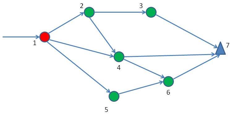
Figure 1: A 7-node network example for routing with recharging nodes.

We formulate a MINLP problem as follows:

$$\min_{x_{ij},r_{i},\,\,i,j\in\mathcal{N}}\quad\sum_{i=1}^{n}\sum_{j=1}^{n}\tau_{ij}x_{ij}+\sum_{i=1}^{n}\sum_{j=1}^{n}r_{i}gx_{ij}$$ (1)

$$s.t.\quad\sum_{j\in O(i)}x_{ij}-\sum_{j\in I(i)}x_{ji}=b_{i},\quad\text{for each }i\in\mathcal{N}$$ (2)

$$b_{1}=1,\,b_{n}=-1,\,b_{i}=0,\text{ for }i\neq 1,n$$ (3)

$$E_{j}=\sum_{i\in I(j)}(E_{i}+r_{i}-e_{ij})x_{ij},\text{ for }j=2,\dots,n$$ (4)

$$0\leq E_{i}\leq B,\quad E_{1}\text{ given},\text{ for each }i\in\mathcal{N}$$ (5)

$$x_{ij}\in\{0,1\},\quad r_{i}\geq 0$$ (6)

where $g$ is the charging time per energy unit, i.e., the reciprocal of a fixed charging rate. The constraints (2)-(3) stand for the flow conservation [[8]], which implies that only one path starting from node $i$ can be selected, i.e., $\sum_{j\in O(i)}x_{ij}\leq 1$. It is easy to check that this also implies $x_{ij}\leq 1$ for all $i,j$ since $b_{1}=1$, $I(1)=\varnothing$. Constraint (4) represents the vehicle’s energy dynamics where the only non-linearity in this formulation appears. Finally, (5) indicates that the vehicle cannot run out of energy before reaching a node or exceed a given capacity $B$. All other parameters are predetermined according to the network topology.

II-A Properties

Rather than directly tackling the MINLP problem, we derive some key properties which will enable us to simplify the solution procedure. The main difficulty in this problem lies in the coupling of the decision variables, $x_{ij}$ and $r_{i}$, in (4). The following lemma will enable us to exclude $r_{i}$ from the objective function by showing that the difference between the total recharging energy and the total energy consumption while traveling is given only by the difference between the vehicle’s residual energy at the destination and at the origin.

Lemma 1: Given (1)-(6),

$$\sum_{i=1}^{n}\sum_{j=1}^{n}(r_{i}x_{ij}-e_{ij}x_{ij})=E_{n}-E_{1}$$ (7)

Proof: From (4), we sum up both sides to get:

$$\sum_{j=2}^{n}E_{j}-\sum_{j=2}^{n}\sum_{i\in I(j)}E_{i}x_{ij}=\sum_{j=2}^{n}\sum_{i\in I(j)}(r_{i}-e_{ij})x_{ij}$$ (8)

Moreover, we can write

$$\sum_{j=2}^{n}\sum_{i\in I(j)}E_{i}x_{ij}=\sum_{i\in I(2)}E_{i}x_{i2}+\cdots+\sum_{i\in I(n)}E_{i}x_{in}$$

representing the sum of $E_{i}$ on the selected path from node $1$ to $n$, excluding $E_{n}$. On the other hand, from (4) we have $E_{i}=0$ for any node $i$ not selected on the path. Therefore, $\sum_{j=2}^{n}E_{j}$ is the sum of $E_{i}$ on the selected path from node $1$ to $n$, excluding $E_{1}$. It follows that

$$\sum_{j=2}^{n}E_{j}-\sum_{j=2}^{n}\sum_{i\in I(j)}E_{i}x_{ij}=E_{n}-E_{1}$$ (9)

Returning to (8), we use (9) and observe that all terms in the double sum $\sum_{i=1}^{n}\sum_{j=1}^{n}(r_{i}-e_{ij})x_{ij}$ are zero except for those with $i\in I(j)$, we get

$$\sum_{i=1}^{n}\sum_{j=1}^{n}(r_{i}-e_{ij})x_{ij}=\sum_{j=2}^{n}\sum_{i\in I(j)}(r_{i}-e_{ij})x_{ij}$$

$$=\sum_{j=2}^{n}E_{j}-\sum_{j=2}^{n}\sum_{i\in I(j)}E_{i}x_{ij}=E_{n}-E_{1}$$

which proves the lemma.$\blacksquare$

In view of Lemma 1, we can replace $\sum_{i=1}^{n}\sum_{j=1}^{n}r_{i}gx_{ij}$ in (1) by $(E_{n}-E_{1})g+\sum_{i=1}^{n}\sum_{j=1}^{n}e_{ij}gx_{ij}$ and eliminate the presence of $r_{i}$, $i=2,\ldots,n-1$, from the objective function. Note that $E_{1}$ is given, leaving us only with the task of determining the value of $E_{n}$. Now, let us investigate the recharging energy amounts $r_{i}^{\ast}$, $i=1,\ldots,n-1$, in an optimal policy. There are two possible cases: $(i)$ $\sum_{i}r_{i}^{\ast}>0$, i.e., the vehicle has to get recharged at least once, and $(ii)$ $\sum_{i}r_{i}^{\ast}=0$, i.e., $r_{i}^{\ast}=0$ for all $i$ and the vehicle has adequate energy to reach the destination without recharging. For Case $(i)$, we establish the following lemma.

Lemma 2: If $\sum_{i}r_{i}^{\ast}>0$ in the optimal routing policy, then $E_{n}^{\ast}=0$.
Proof: We use a contradiction argument. Assume we have already achieved an optimal route where $E_{n}^{\ast}>0$ and the objective function is $J^{\ast}=\sum_{i\in P}(\tau_{i,i+1}+r_{i}^{\ast}g)$ for an optimal path denoted by $P$. Without loss of generality, we re-index nodes so that we may write $P=\{1,\ldots,n\}$. Then, each $i\in P$ such that $i<n$ on this optimal path satisfies:

$$E_{i+1}^{\ast}=E_{i}^{\ast}+r_{i}^{\ast}-e_{i,i+1}$$ (10)

Consider first the case where $r_{n-1}^{\ast}>0$. Let us perturb the current policy as follows: $r_{n-1}^{{}^{\prime}}=r_{n-1}^{\ast}-\Delta$, and $r_{i}^{{}^{\prime}}=r_{i}^{\ast}$ for all $i<n-1$, where $\Delta>0$. Then, from (10), we have

$$E_{n}^{\ast}=E_{1}+\sum_{i=1}^{n-1}(r_{i}^{\ast}-e_{i,i+1})$$

Under the perturbed policy,

$$E_{n}^{{}^{\prime}} =E_{1}+\sum_{i=1}^{n-1}(r_{i}^{{}^{\prime}}-e_{i,i+1})$$

$$=E_{1}+\sum_{i=1}^{n-1}(r_{i}^{\ast}-e_{i,i+1})-\Delta=E_{n}^{\ast}-\Delta$$

$$E_{i}^{{}^{\prime}} =E_{i}^{\ast},\text{ for all }i<n$$

and, correspondingly,

$$J^{{}^{\prime}}=\sum_{i=1}^{n-1}(\tau_{i,i+1}+r_{i}^{{}^{\prime}}\cdot g)=\sum_{i=1}^{n-1}(\tau_{i,i+1}+r_{i}^{\ast}\cdot g)-\Delta g=J^{\ast}-\Delta g$$

Since $E_{n}^{\ast}>0$, we may select $\Delta>0$ sufficiently small so that $E_{n}^{{}^{\prime}}>0$ and the perturbed policy is still feasible. However, $J^{{}^{\prime}}=J^{\ast}-\Delta\cdot g<J^{\ast}$, which leads to a contradiction to the assumption that the original path was optimal.

Next, consider the case where $r_{n-1}^{\ast}=0$. Then, due to $E_{n}^{\ast}>0$ and $e_{i,i+1}>0$ for all $i\in P$, we can always find some $j\in P,$ $j<n$ such that $E_{j}^{\ast}>0$, $r_{j-1}^{\ast}>0$ and $r_{k}^{\ast}=0$ for $k\geqslant j$. Thus, still due to (10), we have

$$E_{j}^{\ast}=E_{n}^{\ast}+\sum_{k=j}^{n-1}e_{k,k+1}>0$$

At this time, since $r_{j-1}^{\ast}>0$, the argument is similar to the case $r_{n-1}^{\ast}>0$, leading again to the same contradiction argument and the lemma is proved. $\blacksquare$

Turning our attention to Case $(ii)$ where $r_{i}^{\ast}=0$ for all $i\in\{1,\ldots,n\}$, observe that the problem (1) can be transformed to

$$\min_{{}_{x_{ij,\text{ }}i,j\in\mathcal{N}}}\quad\sum_{i=1}^{n}\sum_{j=1}^{n}\tau_{ij}x_{ij}$$ (11)

$$s.t.\quad\sum_{j\in O(i)}x_{ij}-\sum_{j\in I(i)}x_{ji}=b_{i},\quad\text{for each }i\in\mathcal{N}$$

$$b_{1}=1,\,b_{n}=-1,\,b_{i}=0,\text{ for }i\neq 1,n$$

$$E_{j}=\sum_{i\in I(j)}(E_{i}-e_{ij})x_{ij},\text{ for }j=2,\dots,n$$ (12)

$$0\leq E_{i}\leq B,\quad E_{0}\text{ given},\text{ for each }i\in\mathcal{N}$$

$$x_{ij}\in\{0,1\}$$ (13)

In this case, the constraint (12) gives

$$\sum_{j=2}^{n}E_{j}-\sum_{j=2}^{n}\sum_{i\in I(j)}E_{i}=-\sum_{j=2}^{n}\sum_{i\in I(j)}e_{ij}x_{ij}$$

Using (9) and $E_{i}\geq 0$, we have

$$E_{n}=E_{1}-\sum_{j=2}^{n}\sum_{i\in I(j)}e_{ij}x_{ij}\geq 0$$

and it follows that

$$\sum_{i=1}^{n}\sum_{j=1}^{n}e_{ij}x_{ij}\leq E_{1}$$ (14)

With (14) in place of (12), the determination of $x_{ij}^{\ast}$ boils down to an integer linear programming problem in which only variables $x_{ij}$, $i,j\in\mathcal{N}$, are involved, a much simpler problem.

We are normally interested in Case $(i)$, where some recharging decisions must be made, so let us assume the vehicle’s initial energy is not large enough to reach the destination. Then, in view of Lemmas 1 and 2, we have the following theorem.

Theorem 1: If $\sum_{i}r_{i}^{\ast}>0$ in the optimal policy, then $x_{ij}^{\ast}$, $i,j\in\mathcal{N}$, in the original problem (1) can be determined by solving a linear programming problem:

$$\min_{{}_{x_{ij,\text{ }}i,j\in\mathcal{N}}}\quad\sum_{i=1}^{n}\sum_{j=1}^{n}(\tau_{ij}+e_{ij}g)x_{ij}$$ (15)

$$s.t.\quad\sum_{j\in O(i)}x_{ij}-\sum_{j\in I(i)}x_{ji}=b_{i},\quad\text{for each }i\in\mathcal{N}$$

$$b_{1}=1,\,b_{n}=-1,\,b_{i}=0,\text{ for }i\neq 1,n$$

$$0\leq x_{ij}\leq 1$$

Proof: Given Lemmas 1 and 2, we know that the optimal solution satisfies $\sum_{i}\sum_{j}r_{i}^{\ast}x_{ij}^{\ast}=\sum_{i}\sum_{j}e_{ij}x_{ij}^{\ast}-E_{1}$. Consequently, we can change the objective (1) to the form below without affecting optimality:

$$\min_{{}_{x_{ij,\text{ }}i,j\in\mathcal{N}}}\quad\sum_{i=1}^{n}\sum_{j=1}^{n}(\tau_{ij}+e_{ij}g)x_{ij}-E_{1}g$$

Since $r_{i}$ no longer appears in the objective function and is only contained in the energy dynamics (4), we can choose any $r_{i}$ satisfying the constraints (4)-(5) without affecting the optimal objective function value. Therefore, $x_{ij}^{\ast}$ can be determined by the following problem:

$$\min_{{}_{x_{ij,\text{ }}i,j\in\mathcal{N}}}\quad\sum_{i=1}^{n}\sum_{j=1}^{n}(\tau_{ij}+e_{ij}g)x_{ij}-E_{1}g$$

$$s.t.\quad\sum_{j\in O(i)}x_{ij}-\sum_{j\in I(i)}x_{ji}=b_{i},\quad\text{for each }i\in\mathcal{N}$$

$$b_{1}=1,\,b_{n}=-1,\,b_{i}=0,\text{ for }i\neq 1,n$$

$$x_{ij}\in\{0,1\}$$

which is a typical shortest path problem formulation. Moreover, according to the property of minimum cost flow problems [[9]], the above integer programming problem is equivalent to the linear programming problem with the integer restriction of $x_{ij}$ relaxed. Finally, since $E_{1}$ is given, the problem reduces to (15), which proves the theorem. $\blacksquare$

II-B Determination of optimal recharging amounts $r_{i}^{\ast}$

Once we determine the optimal route, $P$, in (15), it is relatively easy to find a feasible solution for $r_{i}$, $i\in P$, to satisfy the constraint (4), which is obviously non-unique in general. Then, we can introduce a second objective into the problem, i.e., the minimization of charging costs on the selected path, since charging prices normally vary over stations. As before, we re-index nodes and define $P=\{1,...,n\}$. We denote the charging price at node $i$ by $p_{i}$. Once an optimal route is determined, we seek to control the energy recharging amounts $r_{i}$ to minimize the total charging cost dependent on $p_{i}$, $i\in\mathcal{N}/\{n\}$. This can be formulated as a multistage optimal control problem:

$$\min_{r_{i},\text{ }i\in P}\quad\sum_{i\in P}p_{i}r_{i}$$ (16)

$$s.t.\quad E_{i+1}=E_{i}+r_{i}-e_{i,i+1}$$

$$0\leq E_{i}\leq B,\quad E_{1}\text{ given}$$

$$r_{i}\geq 0\text{ for all }i\in\mathcal{N}$$

This is a simple two-point boundary-value problem and can be easily solved by discrete-time optimal control approaches [[10]] or treating it as a linear programming problem where $E_{i}$ and $r_{i}$ are both decision variables. Due to space limitations, we omit numerical results providing example solutions of the simple linear programming problem (15) and subsequent solutions of (16).

Finally, we note that Theorem 1 holds under the assumption that charging nodes are homogeneous in terms of charging speeds (i.e., the charging rate $1/g$ is fixed). However, our analysis allows for inhomogeneous charging prices. The case of node-dependent charging rates is the subject of ongoing work and can be shown to still allow a decomposition of the MINLP, although we can no longer generally obtain a LP.

III Multiple Vehicle Routing

The results obtained for the single vehicle routing problem pave the way for the investigation of multi-vehicle routing, where we seek to optimize a system-wide objective by routing vehicles through the same network topology. The main technical difficulty in this case is that we need to consider the influence of traffic congestion on both traveling time and energy consumption. A second difficulty is that of implementing an optimal routing policy. In the case of a centrally controlled system consisting of mobile robots, sensors or any type of autonomous vehicles this can be accomplished through appropriately communicated commands. In the case of vehicles with individual drivers, implementation requires signaling mechanisms and possibly incentive structures to enforce desired routes assigned to vehicles, bringing up a number of additional research issues. In the sequel, we limit ourselves to resolving the first difficulty before addressing implementation challenges.

If we proceed as in the single vehicle case, i.e., determining a path selection through $x_{ij}^{k}$, $i,j\in\mathcal{N}$, and recharging amounts $r_{i}^{k}$, $i\in\mathcal{N}/\{n\}$ for all vehicles $k=1,\ldots,K$, for some $K$, then the dimensionality of the solution space is prohibitive. Moreover, the inclusion of traffic congestion effects introduces additional nonlinearities in the dependence of the travel time $\tau_{ij}$ and energy consumption $e_{ij}$ on the traffic flow through arc $(i,j)$, which now depend on $x_{ij}^{1},\cdots,x_{ij}^{K}$. Instead, we will proceed by grouping subsets of vehicles into $N$ “subflows” where $N$ may be selected to render the problem manageable.

Let all vehicles enter the network at the origin node 1 and let $R$ denote the rate of vehicles arriving at this node. Viewing vehicles as defining a flow, we divide them into $N$ subflows (we will discuss the effect of $N$ in Section 3.3), each of which may be selected so as to include the same type of homogeneous vehicles (e.g., large vehicles vs smaller ones or vehicles with the same initial energy). Thus, all vehicles in the same subflow follow the same routing and recharging decisions so that we only consider energy recharging at the subflow level rather than individual vehicles. Note that asymptotically, as $N\rightarrow\infty$, we can recover routing at the individual vehicle level.

Clearly, not all vehicles in our system are BPVs and are, therefore, not part of our optimization process. These can be treated as uncontrollable interfering traffic for our purposes and can be readily accommodated in our analysis, as long as their flow rates are known. However, for simplicity, we will assume here that every arriving vehicle is a BPV and joins a subflow.

Our objective is to determine optimal routes and energy recharging amounts for each subflow of vehicles so as to minimize the total elapsed time of these vehicle flows traveling from the origin to the destination. The decision variables consist of $x_{ij}^{k}\in\{0,1\}$ for all arcs $(i,j)$ and subflows $k=1,\ldots,N$, as well as charging amounts $r_{i}^{k}$ for all nodes $i=1,\ldots,n-1$ and $k=1,\ldots,N$. Given traffic congestion effects, the time and energy consumption on each arc depends on the values of $x_{ij}^{k}$ and the fraction of the total flow rate $R$ associated with each subflow $k$; the simplest such flow allocation is one where each subflow is assigned $R/N$. Let $\mathbf{x_{ij}}=(x_{ij}^{1},\cdots,x_{ij}^{N})^{T}$ and $\mathbf{r_{i}}=(r_{i}^{1},\cdots,r_{i}^{N})^{T}$. Then, we denote the traveling time and corresponding energy consumption of the $k$th vehicle subflow on arc $(i,j)$ by $\tau_{ij}^{k}(\mathbf{x_{ij}})$ and $e_{ij}^{k}(\mathbf{x_{ij}})$ respectively. As already mentioned, $\tau_{ij}^{k}(\mathbf{x_{ij}})$ and $e_{ij}^{k}(\mathbf{x_{ij}})$ can also incorporate the influence of uncontrollable (non-BPV) vehicle flows, which can be treated as parameters in these functions. Similar to the single vehicle case, we use $E_{i}^{k}$ to represent the residual energy of subflow $k$ at node $i$, given by the aggregated residual energy of all vehicles in the subflow. If the subflow does not go through node $i$, then $E_{i}^{k}=0$. The problem formulation is as follows:

$$\min_{\mathbf{x_{ij}},\mathbf{r_{i}},\,\,i,j\in\mathcal{N}}\quad\sum_{i=1}^{n}\sum_{j=1}^{n}\sum_{k=1}^{N}\left(\tau_{ij}^{k}(\mathbf{x_{ij}})+r_{i}^{k}gx_{ij}^{k}\right)$$ (17)

$$s.t.\text{ for each }k\in\{1,\dots,N\}:$$

$$\quad\sum_{j\in O(i)}x_{ij}^{k}-\sum_{j\in I(i)}x_{ji}^{k}=b_{i},\quad\text{for each }i\in\mathcal{N}$$ (18)

$$b_{1}=1,\,b_{n}=-1,\,b_{i}=0,\text{ for }i\neq 1,n$$ (19)

$$E_{j}^{k}=\sum_{i\in I(j)}(E_{i}^{k}+r_{i}^{k}-e_{ij}^{k}(\mathbf{x_{ij}}))x_{ij}^{k},\quad j=2,\dots,n$$ (20)

$$E_{1}^{k}\text{ is given},\quad E_{i}^{k}\geq 0,\quad\text{ for each }i\in\mathcal{N}$$ (21)

$$x_{ij}^{k}\in\{0,1\},\quad r_{i}^{k}\geq 0$$ (22)

Obviously, this MINLP problem is difficult to solve. However, as in the single-vehicle case, we are able to establish some properties that will allow us to simplify it.

III-A Properties

Even though the term $\tau_{ij}^{k}(\mathbf{x_{ij}})$ in the objective function is no longer linear in general, for each subflow $k$ the constraints (18)-(22) are still similar to the single-vehicle case. Consequently, we can derive similar useful properties for this problem in the form of the following two lemmas.

Lemma 3: For each subflow $k=1,\ldots,N$,

$$\sum_{i=1}^{n}\sum_{j=1}^{n}(r_{i}^{k}-e_{ij}^{k}(\mathbf{x_{ij}}))x_{ij}^{k}=E_{n}^{k}-E_{1}^{k}$$ (23)

Lemma 4: If $\sum_{i=1}^{n}r_{i}^{k\ast}>0$ in the optimal routing policy, then $E_{n}^{k\ast}=0$ for all $k=1,\ldots,N$.

The proofs of the above two lemmas are almost identical to those of Lemmas 1 and 2 respectively and are omitted. The only difference is that here the analysis is focused on each vehicle subflow instead of an individual vehicle. In view of Lemma 3, we can replace $\sum_{i=1}^{n}\sum_{j=1}^{n}r_{i}^{k}gx_{ij}^{k}$ in (17) by $(E_{n}^{k}-E_{1}^{k})g+\sum_{i=1}^{n}\sum_{j=1}^{n}e_{ij}^{k}(\mathbf{x_{ij}})gx_{ij}$ and eliminate, for all $k=1,\ldots,N$, the presence of $r_{i}^{k}$, $i=1,\ldots,n-1$, from the objective function similar to the single-vehicle case. Since $E_{1}^{k}$ is given, this leaves only the task of determining the value of $E_{n}^{k}$. There are two possible cases: $(i)$ $\sum_{i}r_{i}^{k\ast}>0$, i.e., the $k$th vehicle subflow has to get recharged at least once, and $(ii)$ $\sum_{i}r_{i}^{k\ast}=0$, i.e., $r_{i}^{k\ast}=0$ for all $i$ and the $k$th vehicle subflow has adequate energy to reach the destination without recharging.

Similar to the derivation of (14), Case $(ii)$ results in a new constraint $\sum_{i}\sum_{j}e_{ij}^{k}(\mathbf{x_{ij}})x_{ij}^{k}\leq E_{1}^{k}$ for subflow $k$. However, since $e_{ij}^{k}(\mathbf{x_{ij}})$ now depends on all $x_{ij}^{1},\ldots,x_{ij}^{N}$, the problem (17)-(22) with all $r_{i}^{k}=0$ is not as simple to solve as was the case with (11)-(13). Let us instead concentrate on the more interesting Case $(i)$ for which Lemma 4 applies and we have $E_{n}^{k\ast}=0$. Therefore, along with Lemma 3, we have for each $k=1,\ldots,N$:

$$\sum_{i=1}^{n}\sum_{j=1}^{n}r_{i}^{k}x_{ij}^{k}=\sum_{i=1}^{n}\sum_{j=1}^{n}e_{ij}^{k}(\mathbf{x_{ij}})x_{ij}^{k}-E_{1}^{k}$$

Then, proceeding as in Theorem 1, we can replace the original objective function (17) and have the following new problem formulation to determine $x_{ij}^{k\ast}$ for all $i,j\in\mathcal{N}$ and $k=1,\ldots,N$:

$$\min_{\mathbf{x_{ij}},\,\,i,j\in\mathcal{N}}\quad\sum_{i=1}^{n}\sum_{j=1}^{n}\sum_{k=1}^{N}\left(\tau_{ij}^{k}(\mathbf{x_{ij}})+e_{ij}^{k}(\mathbf{x_{ij}})gx_{ij}^{k}\right)$$ (24)

$$s.t.\text{ for each }k\in\{1,\dots,N\}:$$

$$\quad\sum_{j\in O(i)}x_{ij}^{k}-\sum_{j\in I(i)}x_{ji}^{k}=b_{i},\quad\text{for each }i\in\mathcal{N}$$

$$b_{1}=1,\,b_{n}=-1,\,b_{i}=0,\text{ for }i\neq 1,n$$

$$x_{ij}^{k}\in\{0,1\}$$

Since the objective function is no longer necessarily linear in $x_{ij}^{k}$, (24) cannot be further simplified into an LP problem as in Theorem 1. The computational effort required to Solve this problem heavily depends on the dimensionality of the network and the number of subflows. Nonetheless, from the transformed formulation above, we are still able to separate the determination of routing variables $x_{ij}^{k}$ from recharging amounts $r_{i}^{k}$. Similar to the single-vehicle case, once the routes are determined, we can obtain any $r_{i}^{k}$ satisfying the energy constraints (20)-(21) such that $E_{n}^{k}=0$, thus preserving the optimality of the objective value. To further determine $r_{i}^{k\ast}$, we can introduce a second level optimization problem similar to the single-vehicle case in (16). Next, we will present an alternative formulation for the original problem (17)-(22) which leads to a computationally simpler solution approach.

III-B Flow control formulation

We begin by relaxing the binary variables in (22) by letting $0\leq x_{ij}^{k}\leq 1$. Thus, we switch our attention from determining a single path for any subflow $k$ to several possible paths by treating $x_{ij}^{k}$ as the normalized vehicle flow on arc $(i,j)$ for the $k$th subflow. This is in line with many network routing algorithms in which fractions $x_{ij}$ of entities are routed from a node $i$ to a neighboring node $j$ using appropriate schemes ensuring that, in the long term, the fraction of entities routed on $(i,j)$ is indeed $x_{ij}$. Following this relaxation, the objective function in (17) is changed to:

$$\min_{\mathbf{x_{ij}},\mathbf{r_{i}},\,\,i,j\in\mathcal{N}}\quad\sum_{i=1}^{n}\sum_{j=1}^{n}\sum_{k=1}^{N}\tau_{ij}^{k}(\mathbf{x_{ij}})+\sum_{i=1}^{n}\sum_{k=1}^{N}r_{i}^{k}g$$

Moreover, the energy constraint (20) needs to be adjusted accordingly. Let $E_{ij}^{k}$ represent the fraction of residual energy of subflow $k$ associated with the $x_{ij}^{k}$ portion of the vehicle flow exiting node $i$. Therefore, the constraint (21) becomes $E_{ij}^{k}\geq 0$. We can now capture the relationship between the energy associated with subflow $k$ and the vehicle flow as follows:

$$\left[\sum_{h\in I(i)}(E_{hi}^{k}-e_{hi}^{k}(\mathbf{x_{ij}}))+r_{i}^{k}\right]\cdot\frac{x_{ij}^{k}}{\sum_{h\in I(i)}x_{hi}^{k}}=E_{ij}^{k}$$ (25)

$$\frac{E_{ij}^{k}}{\sum_{j\in O(i)}E_{ij}^{k}}=\frac{x_{ij}^{k}}{\sum_{j\in O(i)}x_{ij}^{k}}$$ (26)

In (25), the energy values of different vehicle flows entering node $i$ are aggregated and the energy corresponding to each portion exiting a node, $E_{ij}^{k}$ , $j\in O(i)$, is proportional to the corresponding fraction of vehicle flows, as expressed in (26). Clearly, this aggregation of energy leads to an approximation, since one specific vehicle flow may need to be recharged in order to reach the next node in its path, whereas another might have enough energy without being recharged. This approximation foregoes controlling recharging amounts at the individual vehicle level and leads to approximate solutions of the original problem (17)-(22). Several numerically based comparisons are provided in the next section showing little or no loss of optimality relative to the solution of (17).

Adopting this formulation with $x_{ij}^{k}\in[0,1]$ instead of $x_{ij}^{k}\in\{0,1\}$, we obtain the following simpler nonlinear programming problem (NLP):

$$\min_{\mathbf{x_{ij}},\mathbf{r_{i}},\,\,i,j\in\mathcal{N}}\quad\sum_{i=1}^{n}\sum_{j=1}^{n}\sum_{k=1}^{N}\tau_{ij}^{k}(\mathbf{x_{ij}})+\sum_{i=1}^{n}\sum_{k=1}^{N}r_{i}^{k}g$$ (27)

$$s.t.\text{ for each }k\in\{1,\dots,N\}:$$

$$\quad\sum_{j\in O(i)}x_{ij}^{k}-\sum_{j\in I(i)}x_{ji}^{k}=b_{i},\quad\text{for each }i\in\mathcal{N}$$ (28)

$$b_{1}=1,\,b_{n}=-1,\,b_{i}=0,\text{ for }i\neq 1,n$$

$$\left[\sum_{h\in I(i)}(E_{hi}^{k}-e_{hi}^{k}(\mathbf{x_{ij}}))+r_{i}^{k}\right]\cdot\frac{x_{ij}^{k}}{\sum_{h\in I(i)}x_{hi}^{k}}=E_{ij}^{k}$$ (29)

$$\frac{E_{ij}^{k}}{\sum_{j\in O(i)}E_{ij}^{k}}=\frac{x_{ij}^{k}}{\sum_{j\in O(i)}x_{ij}^{k}}$$ (30)

$$E_{ij}^{k}\geq 0,$$ (31)

$$0\leq x_{ij}^{k}\leq 1,\quad r_{i}^{k}\geq 0$$ (32)

As in our previous analysis, we are able to eliminate $\mathbf{r_{i}}$ from the objective function in (27) as follows.

Lemma 5: For each subflow $k=1,\ldots,N$,

$$\sum_{i=1}^{n}r_{i}^{k}=\sum_{i=1}^{n}\sum_{j=1}^{n}e_{ij}^{k}(\mathbf{x_{ij}})+\sum_{i\in I(n)}E_{in}^{k}-\sum_{i\in O(1)}E_{1i}^{k}$$

Proof: Summing (29) over all $i=1,\ldots,n$ gives

$$\sum_{i=1}^{n}r_{i}^{k} =\sum_{i=1}^{n}\sum_{j=1}^{n}e_{ij}^{k}(\mathbf{x_{ij}})+\sum_{i=1}^{n}\sum_{j\in O(i)}E_{ij}^{k}$$

$$\quad-\sum_{i=1}^{n}\sum_{h\in I(i)}E_{hi}^{k}$$

and using (28),(30), we get

$$\sum_{i=1}^{n}r_{i}^{k}=\sum_{i=1}^{n}\sum_{j=1}^{n}e_{ij}^{k}(\mathbf{x_{ij}})+\sum_{i\in I(n)}E_{in}^{k}-\sum_{i\in O(1)}E_{1i}^{k}$$

which proves the lemma. $\blacksquare$

Similar to Lemma 3, we can easily see that if $\sum_{i}r_{i}^{k\ast}>0$ under an optimal routing policy, then $\sum_{i\in I(n)}E_{in}^{k\ast}=0$. In addition, $\sum_{i\in O(1)}E_{1i}^{k}=E_{1}^{k}$, which is given. We can now transform the objective function (27) into (33) and determine the optimal routes $x_{ij}^{k\ast}$ by solving the following NLP:

$$\min_{\begin{subarray}{c}\mathbf{x_{ij}}\\ i,j\in\mathcal{N}\end{subarray}}\quad\sum_{k=1}^{N}\left(\sum_{i=1}^{n}\sum_{j=1}^{n}\left[\tau_{ij}^{k}(\mathbf{x_{ij}})+e_{ij}^{k}(\mathbf{x_{ij}})g\right]-E_{1}^{k}\right)$$ (33)

$$s.t.\text{ for each }k\in\{1,\dots,N\}:$$

$$\quad\sum_{j\in O(i)}x_{ij}^{k}-\sum_{j\in I(i)}x_{ji}^{k}=b_{i},\quad\text{for each }i\in\mathcal{N}$$

$$b_{1}=1,\,b_{n}=-1,\,b_{i}=0,\text{ for }i\neq 1,n$$

$$0\leq x_{ij}^{k}\leq 1$$

The values of $r_{i}^{k}$, $i=1,\ldots,n$, $k=1,\ldots,N$, can be determined so as to satisfy the energy constraints (29)-(31), and they are obviously not unique. We may then proceed with a second-level optimization problem to determine optimal values similar to Section 2.2.

III-C Numerical Examples

We consider a specific example which includes traffic congestion and energy consumption functions. The relationship between the speed and density of a vehicle flow is typically estimated as follows (see [11]):

$$v(k(t))=v_{f}\bigg{(}1-\left(\frac{k(t)}{k_{jam}}\right)^{p}\bigg{)}^{q}$$ (34)

where $v_{f}$ is the reference speed on the road without traffic, $k(t)$ represents the density of vehicles on the road at time $t$ and $k_{jam}$ the saturated density for a traffic jam. The parameters $p$ and $q$ are empirically identified for actual traffic flows. In our multi-vehicle routing problem, we are interested in the relationship between the density of the vehicle flow and traveling time on an arc $(i,j)$, i.e., $\tau_{ij}^{k}(\mathbf{x_{ij}})$. Given a network topology (i.e., a road map), the distances $d_{ij}$ between nodes are known. Moreover, we do not include uncontrollable vehicle flows in our example for simplicity. In our approach, we need to identify $N$ subflows and we do so by evenly dividing the entire vehicle inflow into $N$ subflows, each of which has $R/N$ vehicles per unit time. Thus, $k_{jam}$ in this case can be set as $N$, implying that we do not want all vehicles to go through the same path, hence the the arc $(i,j)$ density is $\sum_{k}x_{ij}^{k}$. Therefore, the time subflow $k$ spends on arc $(i,j)$ becomes

$$\tau_{ij}^{k}(\mathbf{x_{ij}})=\frac{d_{ij}\cdot x_{ij}^{k}\cdot\frac{R}{N}}{v_{f}(1-(\frac{\sum_{k}x_{ij}^{k}}{N})^{p})^{q}}$$

As for $e_{ij}^{k}(\mathbf{x_{ij}})$, we assume the energy consumption rates of subflows on arc $(i,j)$ are all identical, proportional to the distance between nodes $i$ and $j$, giving

$$e_{ij}^{k}(\mathbf{x_{ij}})=e\cdot d_{ij}\cdot\frac{R}{N}$$

Therefore, we aim to solve the multi-vehicle routing problem using (24) which in this case becomes:

$$\min_{\begin{subarray}{c}x_{ij}^{k}\\ i,j\in\mathcal{N}\end{subarray}}\quad\sum_{i=1}^{n}\sum_{j=1}^{n}\sum_{k=1}^{N}\left(\frac{d_{ij}x_{ij}^{k}\frac{R}{N}}{v_{f}(1-(\frac{\sum_{k}x_{ij}^{k}}{N})^{p})^{q}}+egd_{ij}\frac{R}{N}x_{ij}^{k}\right)$$ (35)

$$s.t.\text{ for each }k\in\{1,\dots,N\}:$$

$$\quad\sum_{j\in O(i)}x_{ij}^{k}-\sum_{j\in I(i)}x_{ji}^{k}=b_{i},\quad\text{for each }i\in\mathcal{N}$$

$$b_{1}=1,\,b_{n}=-1,\,b_{i}=0,\text{ for }i\neq 1,n$$

$$x_{ij}^{k}\in\{0,1\}$$

For simplicity, we let $v_{f}=1$ mile/min, $R=1$ vehicle/min, $p=2,\,\,q=2$ and $e\cdot g=1$. The network topology used is that of Fig.1, where the distance of each arc is shown in Tab. I.

TABLE I: $d_{ij}$ values for network of Fig. 1 ($miles$)

$d_{12}$	$d_{14}$	$d_{15}$	$d_{23}$	$d_{24}$	$d_{46}$	$d_{56}$	$d_{37}$	$d_{47}$	$d_{67}$
5	6.2	7	3.5	5	3.6	4.3	6	6	4

To solve the nonlinear binary programming problem (35), we use the optimization solver Opti (MATLAB toolbox for optimization). The results are shown in Tab. II for different values of $N=1,\ldots,30$. As shown in Tab. II, vehicles are mainly distributed through three routes and the traffic congestion effect makes the flow distribution differ from following the shortest path. The number of decision variables (hence, the solution search space) rapidly increases with the number of subflows. However, looking at Fig. 2 which gives the performance in terms of our objective function in (35) as a function of the number of subflows, observe that the optimal objective value quickly converges around $N=10$. Thus, even though the best solution is found when $N=25$, a near-optimal solution can be determined under a small number of subflows. This suggests that one can rapidly approximate the asymptotic solution of the multi-vehicle problem (dealing with individual vehicles routed so as to optimize a systemwide objective) based on a relatively small value of $N$.

TABLE II: Numerical results for sample problem

N	1	2
obj	1.22e9	37.077
routes	$1\rightarrow 4\rightarrow 7$	$\begin{array}[c]{c}1\rightarrow 4\rightarrow 7\\ 1\rightarrow 2\rightarrow 3\rightarrow 7\end{array}$
N	3	4
obj	31.7148	32.8662
routes	$\begin{array}[c]{c}(1\rightarrow 4\rightarrow 7)\\ 1\rightarrow 2\rightarrow 3\rightarrow 7\\ 1\rightarrow 5\rightarrow 6\rightarrow 7\end{array}$	$\begin{array}[c]{c}(1\rightarrow 4\rightarrow 7)\times 2\\ 1\rightarrow 2\rightarrow 3\rightarrow 7\\ 1\rightarrow 5\rightarrow 6\rightarrow 7\end{array}$
N	5	6
obj	32.1921	31.7148
routes	$\begin{array}[c]{c}(1\rightarrow 4\rightarrow 7)\times 2\\ (1\rightarrow 2\rightarrow 3\rightarrow 7)\times 2\\ 1\rightarrow 5\rightarrow 6\rightarrow 7\end{array}$	$\begin{array}[c]{c}(1\rightarrow 4\rightarrow 7)\times 2\\ (1\rightarrow 2\rightarrow 3\rightarrow 7)\times 2\\ (1\rightarrow 5\rightarrow 6\rightarrow 7)\times 2\end{array}$
N	10	15
obj	31.5279	31.4851
routes	$\begin{array}[c]{c}(1\rightarrow 4\rightarrow 7)\times 4\\ (1\rightarrow 2\rightarrow 3\rightarrow 7)\times 3\\ (1\rightarrow 5\rightarrow 6\rightarrow 7)\times 3\end{array}$	$\begin{array}[c]{c}(1\rightarrow 4\rightarrow 7)\times 5\\ (1\rightarrow 2\rightarrow 3\rightarrow 7)\times 5\\ (1\rightarrow 5\rightarrow 6\rightarrow 7)\times 4\\ (1\rightarrow 4\rightarrow 6\rightarrow 7)\times 1\end{array}$
N	25	30
obj	31.4513	31.4768
routes	$\begin{array}[c]{c}(1\rightarrow 4\rightarrow 7)\times 9\\ (1\rightarrow 2\rightarrow 3\rightarrow 7)\times 8\\ (1\rightarrow 5\rightarrow 6\rightarrow 7)\times 7\\ (1\rightarrow 4\rightarrow 6\rightarrow 7)\times 1\end{array}$	$\begin{array}[c]{c}(1\rightarrow 4\rightarrow 7)\times 11\\ (1\rightarrow 2\rightarrow 3\rightarrow 7)\times 10\\ (1\rightarrow 5\rightarrow 6\rightarrow 7)\times 8\\ (1\rightarrow 4\rightarrow 6\rightarrow 7)\times 1\end{array}$

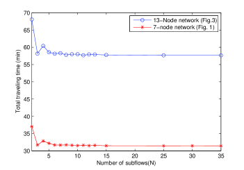
Figure 2: Performance as a function of $N$ (No. of subflows)

Next, we obtain a solution to the same problem (35) using the alternative NLP formulation (33) where $0\leq x_{ij}^{k}\leq 1$. Since in this example all subflows are identical, we can further combine all $x_{ij}^{k}$ over each arc $(i,j)$, which leads to the following $N$-subflow relaxed problem:

$$\min_{x_{ij},\,\,i,j\in\mathcal{N}}\quad\sum_{i=1}^{n}\sum_{j=1}^{n}\left(\frac{d_{ij}x_{ij}R}{v_{f}(1-(x_{ij})^{p})^{q}}+egd_{ij}Rx_{ij}\right)$$ (36)

$$s.t.\quad\sum_{j\in O(i)}x_{ij}-\sum_{j\in I(i)}x_{ji}=b_{i},\quad\text{for each }i\in\mathcal{N}$$

$$b_{1}=1,\,b_{n}=-1,\,b_{i}=0,\text{ for }i\neq 1,n$$

$$0\leq x_{ij}\leq 1$$

This is a relatively easy to solve NLP problem. Using the same parameter settings as before, we obtain the objective value of $31.4465$ mins and the optimal routes are:

$$35.88\%\text{ of vehicle flow: } (1\rightarrow 4\rightarrow 7)$$

$$31.74\%\text{ of vehicle flow: } (1\rightarrow 2\rightarrow 3\rightarrow 7)$$

$$27.98\%\text{ of vehicle flow: } (1\rightarrow 5\rightarrow 6\rightarrow 7)$$

$$4.44\%\text{ of vehicle flow: } (1\rightarrow 4\rightarrow 6\rightarrow 7)$$

Compared to the best solution ($N=25$) in Tab. II and Fig. 2, the difference in objective values between the integer and flow-based solutions is less than $0.1\%$. This supports the effectiveness of a solution based on a limited number of subflows in the MINLP problem.

Performance improvement over uncontrolled traffic systems. Next, we address the extent to which this optimization approach offers improvements over an uncontrolled traffic network. We simulate the vehicle routing problem on the discrete event simulator, MATLAB/SimEvents, where the vehicle arrivals to the source are randomly generated with a random initial energy. As a simple example, we model the routing for each vehicle at each node to be round-robin, while the recharging amount of the vehicle is just adequate to reach the next node. The objective value of such an uncontrolled routing policy for network shown in Fig.1 is $38.524$ mins, compared to our optimal policy which gave $31.451$ mins, an improvement of $18.36\%$.

Larger networks. We have also considered a more topologically complicated network with 13 nodes and 20 arcs as shown in Fig. 3. The number on each arc indicates the distance between adjacent nodes. We assume all other numerical values to be similar to the previous example. Fig. 2 shows the performance in terms of the objective function in (35) vs the number of subflows for this network. We can see that the optimal objective value converges around $N=10$.

Now, let us solve the $N$-subflow relaxed problem (36) for this network with the same parameter settings as before to check for its accuracy. We obtain the optimal objective function value as 57.6326 which is almost equal to the optimal traveling time of 57.6489 obtained for $N=35$ in the MINLP formulation. The optimal routing probabilities are as follows:

$$34.77\%\text{ of vehicle flow: } (1\rightarrow 2\rightarrow 3\rightarrow 4\rightarrow 5\rightarrow 13)$$

$$27.52\%\text{ of vehicle flow: } (1\rightarrow 9\rightarrow 10\rightarrow 11\rightarrow 12\rightarrow 13)$$

$$24.89\%\text{ of vehicle flow: } (1\rightarrow 6\rightarrow 10\rightarrow 7\rightarrow 8\rightarrow 13)$$

$$10.807\%\text{ of vehicle flow: } (1\rightarrow 6\rightarrow 3\rightarrow 8\rightarrow 13)$$

$$1.7\%\text{ of vehicle flow: } (1\rightarrow 9\rightarrow 10\rightarrow 7\rightarrow 8\rightarrow 13)$$

$$0.313\%\text{ of vehicle flow: } (1\rightarrow 6\rightarrow 3\rightarrow 4\rightarrow 5\rightarrow 13)$$

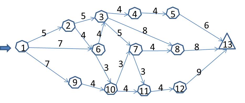
Figure 3: A 13-node network example for routing with recharging nodes.

CPU time Comparison. Based on our simulation results we conclude that the flow control formulation is a good approximation of the original MINLP problem. Tab. III compares the computational effort in terms of CPU time for both formulations to find optimal routes for the two sample networks we have considered. Our results show that the flow control formulation results in a reduction of about 5 orders of magnitude in CPU time with virtually identical objective function values.

TABLE III: CPU time for sample problems

Fig.1 Net.	MINLP	MINLP	NLP approx.
N	2	10(near opt)	-
obj	37.083	31.5319	31.4504
CPU time(sec)	312	9705	0.07
Fig.3 Net.	MINLP	MINLP	NLP approx.
N	2	15(near opt)	-
obj	68.055	57.764	57.6326
CPU time(sec)	820	10037	0.2

Effect of recharging speed on optimal routes. Once we determine the optimal routes, we can also ascertain the total time spent traveling and recharging respectively, i.e., the first and second terms in (36). Obviously the value of $e\cdot g$, which captures the recharging speed, determines the proportion of traveling and recharging amount as well as the route selection. As shown in Tab. IV, the larger the product $e\cdot g$ is, the slower the recharging speed, therefore the more weighted the recharging time in the objective function becomes. In this case, flows tend to select shortest paths in terms of energy consumption. Conversely, if the recharging speed is fast, the routes are selected to prioritize the traveling time on paths.

TABLE IV: Numerical results for different values of $e\cdot g$ for network of Fig. 1

$e\cdot g$	0.1	1	10
total time	18.9417	31.4465	154.4777
time on paths	17.5471	17.5791	19.4510
time at stations	1.3946	13.8674	135.0267
optimal routes	$\begin{array}[c]{cl}31.53\%:&(1\rightarrow 2\rightarrow 3\rightarrow 7)\\ 32.97\%:&(1\rightarrow 4\rightarrow 7)\\ 28.58\%:&(1\rightarrow 5\rightarrow 6\rightarrow 7)\\ 5.78\%:&(1\rightarrow 4\rightarrow 6\rightarrow 7)\\ 1.14\%:&(1\rightarrow 2\rightarrow 4\rightarrow 7)\end{array}$	$\begin{array}[c]{cl}31.74\%:&(1\rightarrow 2\rightarrow 3\rightarrow 7)\\ 35.88\%:&(1\rightarrow 4\rightarrow 7)\\ 27.98\%:&(1\rightarrow 5\rightarrow 6\rightarrow 7)\\ 4.4\%:&(1\rightarrow 4\rightarrow 6\rightarrow 7)\end{array}$	$\begin{array}[c]{cl}32.35\%:&(1\rightarrow 2\rightarrow 3\rightarrow 7)\\ 49.63\%:&(1\rightarrow 4\rightarrow 7)\\ 18.02\%:&(1\rightarrow 5\rightarrow 6\rightarrow 7)\end{array}$

IV Conclusions and future work

We have introduced energy constraints into the vehicle routing problem, and studied the problem of minimizing the total elapsed time for vehicles to reach their destinations by determining routes as well as recharging amounts when there is no adequate energy for the entire journey. For a single vehicle, we have shown how to decompose this problem into two simpler problems. For a multi-vehicle problem, where traffic congestion effects are considered, we used a similar approach by aggregating vehicles into subflows and seeking optimal routing decisions for each such subflow. We also developed an alternative flow-based formulation which yields approximate solutions with a computational cost reduction of several orders of magnitude, so they can be used in problems of large dimensionality. Numerical examples show these solutions to be near-optimal. We have also found that a low number of subflows is adequate to obtain convergence to near-optimal solutions, making the multi-subflow strategy particularly promising.

Our ongoing work introduces different characteristics into the charging stations, such as recharging speeds and queueing capacities. In this case, we can show that a similar decomposition still holds, although we can no longer obtain an LP problem. We also believe that extensions to multiple vehicle origins and destinations are straight-forward, as is the case where only a subset of nodes has recharging resources or not all vehicles in the network are BPVs. Finally, we are exploring extensions into stochastic vehicle flows which can incorporate various random effects.

References

- [1] G. Laporte, “The vehicle routing problem: An overview of exact and approximate algorithms,” European Journal of Operational Research, vol. 59, 1992.
- [2] A. Artmeier, J. Haselmayr, M. Leucker, and M. Sachenbacher, “The optimal routing problem in the context of battery-powered electric vehicles,” in Workshop: CROCS at CPAIOR-10, 2nd International Workshop on Constraint Reasoning and Optimization for Computational Sustainability, Bologna, Italy, May 2010.
- [3] J. Eisner, S. Funke, and S. Storandt, “Optimal route planning for electric vehicles in large networks,” in Proceedings of the 25th AAAI Conference on Artificial Intelligence, San Francisco, US, Aug. 2011.
- [4] U. F. Siddiqi, Y. Shiraishi, and S. M. Sait, “Multi-constrained route optimization for electric vehicles (evs) using particle swarm optimization,” in 2011 11th International Conference on Intelligent Systems Design and Application (ISDA), Cordoba, Spain, Nov. 2011, pp. 391–396.
- [5] S. Khuller, A. Malekian, and J. Mestre, “To fill or not to fill: The gas station problem,” ACM Transactions on Algorithms, vol. 7, 2011.
- [6] M. Schneider, A. Stenger, and D. Goeke, “The electric vehicle routing problem with time windows and recharging stations,” Tech Report, Dept. of Business Information Systems and Operations Research, University of Kaiserslautern, www.wiiw.de/publikationen/TheElectricVehicleRoutingProbl4278.pdf, 2012.
- [7] K. Sunder and S. Rathinam, “Route planning algorithms for unmanned aerial vehicles with refueling constraints,” in 2012 American Control Conference (ACC), Montreal,Canada, Nov. 2012, pp. 3266–3271.
- [8] D. Bertsimas and J. N. Tsitsiklis, Introduction to Linear Programming. Athena Scientific, 1997.
- [9] F. S. Hillier and G. J. Lieberman, Introduction to operations research eighth edition. McGraw-Hill, 2005.
- [10] A. E. Bryson and Y. Ho, Applied Optimal Control. Washington D.C.: Hemisphere Publ. Corp., 1975.
- [11] F. Ho and P. Ioannou, “Traffic flow modeling and control using artificial neural networks,” Control Systems, IEEE, vol. 16, pp. 16 – 26, 1996.