2 Department of Astronomy and Space Science, Sejong University, Seoul, 143-747, Korea
3 Lawrence Berkeley National Laboratory, Berkeley, CA 94720, USA
4 INAF, Osservatorio Astronomico di Trieste, via G. B. Tiepolo 11, 34131 Trieste, Italy
5 INFN/National Institute for Nuclear Physics, via Valerio 2, 34127 Trieste, Italy
6 School of Physics and Astronomy, University of Nottingham, University Park, Nottingham NG7 2RD
Suite of hydrodynamical simulations for the Lyman-alpha forest with massive neutrinos
The signature left in quasar spectra by neutral hydrogen in the Universe allows constraining the sum of the neutrino masses with a better sensitivity than laboratory experiments and may shed new light on the neutrino mass hierarchy and the absolute mass-scale of neutrinos. Constraints on cosmological parameters and on the dark energy equation of state can also be derived from a joint parameter estimation procedure. However, this requires a detailed modeling of the line-of-sight power spectrum of the transmitted flux in the Lyman- (Ly) forest on scales ranging from a few to hundreds of megaparsecs, which in turn demands the inclusion and careful treatment of cosmological neutrinos. To this end, we present here a suite of state-of-the-art hydrodynamical simulations with cold dark matter (CDM), baryons and massive neutrinos, specifically targeted for modeling the low-density regions of the intergalactic medium (IGM) as probed by the Ly forest at high-redshift. The simulations span volumes ranging from to , and were made using either million or billion particles. The resolution of the various runs was further enhanced, so that we reached the equivalent of billion particles in a box size. The chosen cosmological parameters are compatible with the latest Planck (2013) results, although we also explored the effect of slight variations in the main cosmological and astrophysical parameters. We adopted a particle-type implementation of massive neutrinos, and consider three degenerate species with masses , and eV, respectively. We improved on previous studies in several ways, in particular with updated routines for IGM radiative cooling and heating processes, and initial conditions based on second-order Lagrangian perturbation theory (2LPT) rather than the Zel’dovich approximation. This allowed us to safely start our runs at relatively low redshift (), which reduced the shot-noise contamination in the neutrino component and the CPU consumption. In addition to providing technical details on the simulations, we present the first analysis of the nonlinear three- and one-dimensional matter and flux power spectra from these models, and characterize the statistics of the transmitted flux in the Ly forest including the effect of massive neutrinos. In synergy with recent data from the Baryon Acoustic Spectroscopic Survey (BOSS) and the Planck satellite, and with a grid of corresponding neutrino-less simulations, our realizations will allow us to constrain cosmological parameters and neutrino masses directly from the Ly forest with improved sensitivity. In addition, our simulations can be useful for a broader variety of cosmological and astrophysical applications, ranging from the three-dimensional modeling of the Ly forest to cross-correlations between different probes, studying the expansion history of the Universe including massive neutrinos, and particle-physics related topics. Moreover, while our simulations have been specifically designed to meet the requirements of the BOSS survey, they can also be used for upcoming or future experiments – such as eBOSS and DESI.
Key Words.:
large-scale structure of Universe – cosmology: theory, observations, numerical simulations, intergalactic medium, neutrinos – methods: numerical1 INTRODUCTION
Neutrino science has received a boost of attention recently, because the breakthrough discovery in particle physics over the last decade that neutrinos are indeed massive. However, at the present time we only know their mass differences, because solar, atmospheric, reactor, and accelerator observations of neutrino oscillations are sensitive only to differences in the squares of neutrino masses, requiring that there be at least one species with mass eV. On the other hand, cosmology offers a unique ‘laboratory’ with the best sensitivity to the neutrino mass (see for example Lesgourgues & Pastor 2012, and references therein), as primordial massive neutrinos comprise a small portion of the dark matter (DM) and therefore must significantly alter structure formation. Potentially, combining cosmological and particle physics results, it is expected that we will be able to determine the absolute mass scale of neutrinos in the very near future, and solve one of the key questions in neutrino physics today – namely, the nature of their mass hierarchy and perhaps the origin of mass.
Neutrino physics also provides one of the best examples of the interplay between particle physics and cosmology/astrophysics. For instance, the measurement of neutrino masses could point to a new fundamental theory, of which the standard model (SM) is the low-energy limit (Lesgourgues & Pastor 2006) – hence calling for new physics beyond the SM. In addition, astrophysical neutrino fluxes can be exploited to test the SM, with experiments of neutrino decays, oscillations, and searches for nonzero neutrino electromagnetic moments.
In a cosmological context, the effect of massive neutrinos is essentially twofold. Firstly, neutrinos contribute to the expansion rate during the radiation epoch as one of neutrinos (with the effective number of neutrino species; a recent constraint from the Planck data is – see Ade et al. 2013) and later as a nonrelativistic component of matter. Compared with massless models, this modifies the timing of matter-radiation equality and the distance-redshift relation. Secondly, after they become non-relativistic, neutrinos participate in structure formation, but only on scales greater than the free-streaming scale. Because of these two effects, models with neutrino masses greater than eV give predictions different from standard cold dark matter (CDM) scenarios with a cosmological constant (i.e., LCDM models), which generally incorporate a minimal neutrino mass of eV.
Hence, while the most recent results from the cosmic microwave background (CMB), such as data from the Planck satellite (Ade et al. 2013), the Atacama Cosmology Telescope (ACT; Sievers et al. 2013) or the South Pole Telescope (SPT; Hou et al. 2012), and from the large-scale structure (LSS) as in the Sloan Digital Sky Survey (SDSS; York et al. 2000, Eisenstein et al. 2011) or in the WiggleZ survey (Drinkwater et al. 2010; Blake et al. 2012) are consistent with the CDM model dominated by a dark energy (DE) component, with baryons constituting only of the total matter-energy content, a pure CDM scenario is still unsatisfactory and incomplete – since even a small amount of neutrinos can significantly impact structure formation. Improving our knowledge of cosmological neutrinos is essential for an accurate and consistent minimal cosmological model, and the present study is an effort in this direction.
In cosmology, neutrinos have been studied with a large number of probes and complementary techniques. The most direct way is through the analysis of the CMB radiation, because for the current mass limits their primordial signature does not vanish although neutrinos are still relativistic at the time of recombination (Lesgourgues & Pastor 2006). While the overall sensitivity of massive neutrinos impacts the CMB temperature power spectrum very marginally, there are non-negligible consequences in the polarization maps through the early integrated Sachs Wolfe (ISW) effect (Hinshaw et al. 2013), and distinct signatures from the gravitational lensing of the CMB by LSS – both in temperature and polarization (see for instance Santos et al. 2013 or Battye & Moss 2013). Other methods for quantifying the impact of massive neutrinos involve baryonic tracers of the LSS clustering of matter, and high-redshift surveys. Examples include the measurement of the three-dimensional matter power spectrum obtained from galaxy surveys, Lyman- (Ly), or cm probes where the underlying tracer is neutral hydrogen (HI), the study of galaxy clusters via the Sunyaev-Zel’dovich (SZ) effect, and the characterization of the cosmic shear through weak lensing (Kaiser 1992; Jain & Seljak 1997; Zaldarriaga & Seljak 1998; Abazajian & Dodelson 2003).
While most techniques used in cosmology to constrain neutrino masses are based on the CMB or on galaxy clustering, fewer studies involve the Ly forest – that is, the absorption lines in the spectra of high-redshift quasars, that are due to neutral hydrogen in the intervening photoionized intergalactic medium (IGM). Thanks to data from the SDSS (York et al. 2000), the statistical power of the Ly forest has greatly increased, so that it is now emerging as a very promising and unique window into the high-redshift Universe, because it is at a redshift range inaccessible to other LSS probes and spans a wide interval in redshift. For this reason, it was recently possible, for instance, to detect for the first time the baryon acoustic oscillation (BAO) signal directly from the Ly forest (Busca et al. 2013; Slosar et al. 2013). This will be even more so with future surveys, such as eBOSS (Comparat et al. 2013) and DESI (Schlegel et al. 2011).
The Ly forest is particularly well suited to constrain neutrino masses, since massive neutrinos leave a redshift- and mass-dependent signature in the one-dimensional flux power spectrum because the growth of cosmological structures on scales smaller than the neutrino free-streaming distance is suppressed. To detect this effect, careful modeling of the line-of-sight (LOS) power spectrum of the transmitted Ly flux is required. Pioneering work along these lines has been carried out by Croft et al. (1998, 2002), Zaldarriaga, Hui & Tegmark (2001), Viel et al. (2004, 2006, 2010), Seljak et al. (2005), McDonald et al. (2006), Seljak, Slosar & McDonald (2006), and Kim & Croft (2008). In particular, McDonald et al. (2006) and Seljak et al. (2006) used a sample of moderate-resolution forest spectra from the SDSS to measure the one-dimensional flux power spectrum at . They placed constraints on the linear matter power spectrum and on neutrino masses, while Viel et al. (2010) studied the impact of massive neutrinos in the transmitted Ly flux. At present, the most precise measurement of the Ly flux power spectrum comes from the Baryon Acoustic Spectroscopic Survey (BOSS; Dawson et al. 2013), with a sample of forest spectra almost two orders of magnitude larger than in previous studies (Palanque-Delabrouille et al. 2013). These Ly forest measurements supplement those obtained from the population of luminous red galaxies (LRGs), and considerably extend the redshift range that can be studied.
The Ly forest also offers one of the strongest reported constraints on neutrino mass when combined with WMAP 3-year CMB data (i.e. eV at 95% CL; Seljak et al. 2006), but the constraint depends on the normalization of the observed LSS power spectrum relative to the CMB power spectrum; using recent data from the Planck satellite instead of those from WMAP, the previous constraints are weakened. Nevertheless, current neutrino mass limits are on the verge of distinguishing between a normal (one species with eV) and inverted (two species with eV) hierarchy, and in the near future the degeneracy of neutrino masses will be removed by combining cosmological results with atmospheric and solar neutrino constraints. For example, the combination of Planck CMB data, WMAP 9-year CMB polarization data (Bennett et al. 2013), and a measurement of BAO from BOSS, SDSS, WiggleZ, and the 6dF galaxy redshift survey (Jones et al. 2009) produces an upper limit of (95% CL), while a more aggressive use of galaxy clustering into smaller scales and the nonlinear clustering regime can lead to stringent constraints (Zhao et al. 2012; Riemer-Sørensen et al. 2013).
However, the validity of the current limits on neutrino masses depends on the assumption that there are no systematic offsets between estimates of the matter power spectrum obtained with different methods; according to Viel et al. (2010), these uncertainties are not reflected in the quoted measurement errors. To this end, one needs to gain a better understanding of the characteristic signatures of massive neutrinos in the power spectrum across different redshift slices, and be in control of the various systematics involved, especially at lower redshifts () and at small scales (Mpc) – where the nonlinear evolution of density fluctuations for massive neutrinos is non-negligible. Particularly for the Ly forest, constraints on neutrino masses are only limited by the systematic accuracy with which we can make these theoretical predictions. This is only possible through more and more sophisticated numerical simulations, where the full hydrodynamical treatment is performed at scales where nonlinear effects become important for the neutrino component; so far, only a handful studies in the literature have addressed these aspects for the Ly forest in some detail. Given that current and planned experiments such as BOSS, eBOSS and DESI will provide excellent-quality data for the Ly forest (see also the recent American 2013 report ‘Cosmic Frontier Vision’, and in particular Connolly et al. 2013), it is now timely to design and perform accurate numerical simulations capable of reproducing the effects of massive neutrinos.
The present study aims at filling this gap by presenting a suite of state-of-the-art hydrodynamical simulations with cold dark matter, baryons and massive neutrinos, specifically targeted for modeling the low-density regions of the IGM as probed by the Ly forest at high-redshift. In addition to providing technical details on the simulations and on the improvements made with respect to pre-existing literature, we show here measurements of the simulated nonlinear three- and one-dimensional matter and flux power spectra, and characterize the statistics of the transmitted flux in the Ly forest in presence of massive neutrinos. This is the first of a series of papers dedicated to quantify the effects of massive neutrinos in the Ly forest across different redshift slices and at nonlinear scales. In addition, we are planning to make the simulations available to the scientific community upon request; hence, the present work may serve as a guide for a direct use of the simulations and of the products provided.
The layout of the paper is organized as follows: in Section 2, we briefly outline the theory behind the modeling of the Ly forest, along with the most commonly used numerical techniques available. In Section 3, we focus on neutrino science and on the implementation of massive neutrinos in cosmological -body simulations and explain the method of our choice. In Section 4, we present our novel suite of hydrodynamical simulations and provide several technical details on the code used for the run, initial conditions, optimization strategies and performance, along with various improvements and a description of the pipeline developed to extract the synthetic Ly transmitted flux; in the appendix, we also describe a sanity check we performed to ensure that we correctly recover the limit of massless neutrinos. In Section 5, we present the first analysis of our suite of simulations, where in particular we compute the three- and one-dimensional matter and flux power spectra, focusing on the imprint of massive neutrinos. We conclude in Section 6, where we summarize our main achievements and explain how we will use the simulations presented here to constrain neutrino masses directly from the Ly forest, with improved sensitivity.
2 MODELING THE LYMAN-ALPHA FOREST
In this section we briefly summarize the basic theory of the Ly forest as a cosmological probe and the most commonly used numerical techniques for modeling the low-density regions of the IGM. In particular, we focus on the specific requirements necessary to accurately reconstruct the Ly transmitted flux.
2.1 Ly forest: overview and challenges
The observational discovery of the Ly forest traces back to Lynds (1971), although the actual existence of an ionized IGM was already postulated back in the 1960s (Bahcall & Salpeter 1965; Gunn & Peterson 1965). However, only some twenty years later was it realized that the numerous absorption features in the spectra of high-redshift quasars, bluewards of the redshifted resonant Å emission line, directly trace the underlying dark matter fluctuations (Cen et al. 1994; Bi et al. 1995; Zhang et al. 1995; Hernquist et al. 1996; Miralda-Escude et al. 1996; Bi & Davidsen 1997; Hui, Gnedin & Zhang 1997; Theuns et al. 1998). Clearly, since hydrogen makes up most of the baryonic density of the Universe, the Ly forest is also a direct tracer of the baryonic matter distribution over a wide range of scales and redshifts – i.e. ; .
Since then, considerable progress has been made toward a thorough understanding of the nature of these absorption features and of the properties of the IGM. We now have observational evidence that at high redshift the IGM contains the majority of baryons present in the Universe (Petitjean et al. 1993; Fukugita et al. 1998), is highly ionized by the ultra-violet (UV) background produced by galaxies and quasars, and becomes increasingly neutral from to (Mortlock et al. 2011). The overall physical picture that emerges is relatively simple: the IGM probed by the Ly forest consists of mildly nonlinear gas density fluctuations; low column-density absorption lines trace the filaments of the cosmic web; high column-density absorption lines trace the surrondings of galaxies; the gas traces the dark matter, and is photoionized and photoheated by the UV-background. Although metals are present in the IGM (Cowie et al. 1995; Schaye et al. 2003; Aracil et al. 2004), stirring of the IGM due to feedback from galaxies or active galactic nuclei (AGNs) does not significantly affect the vast majority of the baryons (Theuns et al. 2002; McDonald et al. 2005). Photoionization heating and expansion cooling cause the gas density () and temperature () to be closely related, except where mild shocks heat the gas (see Schaye et al. 2000), so that in low-density regions a simple redshift-dependent polytropic power-law temperature-density relation holds (Katz, Weinberg & Hernquist 1996; Hui & Gnedin 1997):
| (1) |
where and are the corresponding gas mean temperature and density, while the parameter depends on redshift, reionization history model, and spectral shape of the UV background. It is interesting to address the modifications to this simple relation caused by massive neutrinos, and we return to this issue in Section 5.
The gas of the IGM is generally assumed to be in photoionization equilibrium with the UV background, and it can be described by an optical depth that depends on the evolving photoionization rate (Peebles 1993). The optical depth for Ly absorption is proportional to the neutral hydrogen density (Gunn & Peterson 1965), which – since the gas is in photoionization equilibrium – can also be expressed as
| (2) |
where and depends on redshift, baryon density, temperature at the mean density, Hubble constant, and photoionization rate. While the optical depth is a tracer of the matter distribution on scales larger than the Jeans length of the photoionized IGM, it is more conventional to use the mean transmitted flux instead, and define an effective optical depth so that
| (3) |
The previous expression contains the uncertainties in the intensity of the UV background, the mean baryon density, and other parameters that set the normalization of the relation between optical depth and density of the gas. Measurements of the mean transmission and of its evolution allow one to constrain the basic cosmological parameters (see Jenkins & Ostriker 1991; Hernquist et al. 1996; Rauch et al. 1997; Rauch 1998; McDonald & Miralda-Escude 2001). The gas density is also closely related to that of the DM on large scales, while on small scales the effects of thermal broadening and Jeans smoothing must be included. For more details on the physics of the IGM and its potential for cosmology, see Meiksin (2009).
Dynamical and thermal processes are essential in modeling the Ly forest: therefore, the effects of baryon pressure, nonlinear evolution of density perturbations, thermal and chemical evolution such as adiabatic cooling due to the expansion of the Universe, UV background photoionization heating, as well as Compton and recombination cooling need to be taken into account. For instance, the Ly flux power spectrum depends not only on the DM distribution, but also on the thermal state of the IGM, and on feedback effects due to star formation and AGNs. Hence, a full hydrodynamical modeling including effects of galaxy formation physics is necessary. While there exist several numerical challenges in simulating the Ly forest, along with a series of physical mechanisms still poorly understood, today we do have the computational capability of carrying out full hydrodynamical treatments, as we perform in this work. Despite hydrodynamic uncertainties, hierarchical models of structure formation are now capable of reproducing almost all the aspects of the Ly forest. We also note that once the spectrum is modeled as a continuous phenomenon, there is no need to resolve every single feature (Weinberg et al. 1999, 2003), so that the forest can be studied with relatively moderate resolution spectra.
2.2 Hydrodynamical simulations in a nutshell
The rapid progress made in our theoretical understanding of the Ly forest is mainly due to the improved ability to simulate all the physical effects that impact the IGM more and more realistically – thanks to state-of-the-art computational facilities. In fact, while the forest has been traditionally studied using a variety of analytical techniques such as the Zel’dovich approximation (Doroshkevich & Shandarin 1977; McGill 1990; Hui, Gnedin & Zhang 1997; Matarrese & Mohayaee 2002), the lognormal approximation (Hamilton 1985; Coles & Jones 1991; Bi 1993; Bouchet et al. 1993; Kofman et al. 1994; Gnedin & Hui 1996; Bi & Davidsen 1997; Viel et al. 2002), or semi-analytic models (Balian & Schaeffer 1989; Bernardeau & Schaeffer 1992, 1999; Valageas, Schaeffer & Silk 1999; Pichon et al. 2001), it is only with hydrodynamical simulations that the interplay between gravity and gas pressure on the structure of the photoionized IGM can be modeled self-consistently – so that most of the observed properties of the Ly forest are successfully reproduced and the uncertainties in the theoretical modeling overcome.
Traditionally, cosmological hydro-simulations come in two basic flavors: smoothed particle hydrodynamics (SPH; Gingold & Monaghan 1977; Lucy 1977), and grid-based methods; there are also more sophisticated combinations of the two categories. The SPH technique – adopted in this study – uses particles to represent the baryonic fluid, employs an artificial viscosity to simulate shocks (Springel & Hernquist 2002), and it is Lagrangian in nature: this implies that the resolution is concentrated in regions of high-density. On the other hand, grid-based methods use a grid of cells to represent the gas properties, which may provide a superior resolution of the low-density regions of the IGM and more accurate treatments of shocks, but at a higher computational cost. For more details on hydrodynamical techniques relevant to this study, see Katz et al. (1996).
Both approaches have been successfully used to model the Ly forest at low- and high-redshift and to obtain quantitative estimates of the clustering amplitude and constraints on cosmological and astrophysical parameters. The number of dedicated studies has increased in recent years, since the forest is emerging as a key probe of the hydrogen reionization epoch. A long, but still incomplete list of relevant numerical works includes Gnedin & Hui (1996, 1998), Croft et al. (1998, 1999, 2002), Hui et al. (2001), McDonald et al. (2000, 2001, 2005), Meiksin & White (2001), Gnedin & Hamilton (2002), Zaldarriaga et al. (2001, 2003), Seljak et al. (2003), Bolton & Haehnelt (2007), Viel et al. (2003, 2004, 2010, 2012), Crain et al. (2009), Bolton & Becker (2009), Schaye et al. (2010).
The importance of having full hydrodynamical simulations cannot be stressed enough. To provide an example, McDonald et al. (2005) used hydrodynamical simulations extended with hydro-particle-mesh (HPM) realizations to analyze the SDSS Ly forest power spectrum and infer the corresponding linear theory power spectrum. However, their HPM simulations – calibrated by a limited number of hydrodynamical runs – were found to be discrepant by up to when compared with full hydrodynamical simulations, with respect to the statistical properties of the Ly flux distribution (Viel et al. 2006). Hence, while using approximate numerical calculations is certainly attractive because computationally less demanding, a complete hydrodynamical treatment is mandatory to reach the precision that data are now beginning to show.
Before moving on to the treatment of massive neutrinos, we stress that the development of progressively more sophisticated numerical simulations is an area of rapid progress – particularly crucial for a realistic modeling of the Ly forest. With increasing computational power, there is currently less motivation to use approximation methods – although more work is needed to understand a multitude of complex baryonic processes. This is even more so when massive neutrinos are included in the picture, and the scope of the present work is to add more knowledge in this direction.
3 IMPLEMENTING MASSIVE NEUTRINOS
In this section we first provide a synthetic overview of the effects of massive neutrinos in cosmology – focusing on the Ly forest; in particular, we present the expected linear predictions for the matter power spectra in presence of massive neutrinos, with the set of cosmological parameters adopted in our simulations. We then briefly describe how neutrinos are implemented. In Section 5, the linear predictions shown here are compared with nonlinear measurements obtained from our simulations.
3.1 Revival of neutrino science
The impact of massive neutrinos on the CMB and LSS was investigated long ago (see for example Bond, Efstathiou & Silk 1980; Klypin et al. 1993; Ma & Bertschinger 1995; Dodelson et al. 1996; Hu, Eisenstein & Tegmark 1998; Hu & Dodelson 2002; Abazajian et al. 2005; Hannestad 2005; Seljak et al. 2006), and with a renewed interest quite recently (e.g. Saito et al. 2008, 2009; Wong 2008; Brandbyge et al. 2008; Brandbyge & Hannestad 2009; Viel et al 2010; Marulli et al. 2011; Bird et al 2012; Carbone et al. 2012; Hou et al. 2012; Lesgourgues & Pastor 2012). The renewed interest is mainly driven by the large amount of cosmological data available today, which allow placing competitive limits on the neutrino mass-scale and hierarchy. For instance, simply with the improvement of a factor of two from Seljak et al. (2006), one should be able to distinguish between a normal hierarchy and an inverted one – a fact within reach in the very near future, given high-quality upcoming surveys such as eBOSS and DESI.
The effects of cosmological neutrinos on the evolution of density perturbations in the linear regime is well understood. In what follows, we only discuss a few general aspects of cosmological neutrinos relevant for the Ly forest, and refer to Lesgourgues & Pastor (2006, 2012) for a more exhaustive treatment.
Neutrinos decouple from the cosmic plasma before the electron-positron annihilation (around MeV), resulting in a subsequent neutrino temperature that is lower than the photon temperature , namely
| (4) |
and a number density lower than the photon number density:
| (5) |
where is the density of the CMB photons, and the factor 3/4 comes from the difference between the Fermi-Dirac and Bose-Einstein statistics. Moreover, they behave as additional radiation while ultra-relativistic, traveling at the speed of light with a free-streaming length equal to the Hubble radius, and as an additional CDM component when they become non-relativistic. Subsequently, massive neutrinos affect structure formation by free-streaming and by delaying matter domination. These effects can be parameterized by their ultimate fractional contribution to the matter density:
| (6) |
where is the present value of the Hubble constant in units of 100 km , is the sum of the neutrino masses of the three species considered, and is the matter energy density in terms of the critical density.
Neutrinos in the mass range become non-relativistic in the redshift interval , approximately around /1eV) – during the matter domination era; for the given mass-intervals considered in this study, all our runs started well in the non-relativistic regime. When neutrinos are non-relativistic, there is a minimum wavenumber
| (7) |
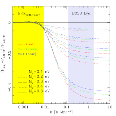
above which the physical effect produced by their free-streaming damps small-scale density fluctuations, while modes with evolve according to linear theory. The free-streaming leads to a suppression of power on small scales; with increasing neutrino mass, this suppression becomes stronger and its shape and amplitude depend mainly on the total mass, but only weakly on redshift (Bond, Efstathiou & Silk 1980). At scales the suppression is constant, while at it gradually decreases to zero – with expressed in units of . When (very large scales), the influence of neutrinos in the matter power spectrum becomes negligible. All these effects are clearly seen in Figure 1, where we show the linear theory predictions for the matter power spectra, which include massive neutrinos (), normalized by the corresponding case of massless neutrinos (). The cosmological parameters adopted are those used for our simulations and reported in Section 4; we consider the following neutrino masses: eV. With different colors but similar line styles, we also show the evolution in redshift for three significant intervals, namely (red), (green), and (blue). All the various linear predictions were computed with the CAMB code (Lewis, Challinor & Lasenby 2000). The yellow area in the figure corresponds to values of lower than for eV (i.e., the most massive case considered here) obtained from (7), below which a linear description for the neutrino evolution is sufficient. For masses eV, the corresponding values are lower than . The gray area in the same figure shows the -range approximately covered by the BOSS survey, relatively to the one-dimensional Ly forest power spectrum. As can be clearly seen, our primary range of interest lies well outside the zone in which a linear description would be sufficient – for the neutrino masses considered in this study; hence, a full nonlinear treatment of the neutrino component is mandatory. In Section 5, we compare these linear predictions with the corresponding nonlinear evolutions as a function of neutrino mass and quantify the departures from linearity; we also determine at which these departures are maximized.
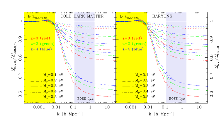
Figure 2 presents the dimensionless linear power spectra per component when massive neutrinos are included, normalized by the corresponding zero-neutrino-mass case. The general convention used in this paper sets , where the subscript specifies the component considered. In detail, the left panel shows the CDM linear evolution, while the right panel displays the evolution of the baryonic component; neutrino mass ranges, redshifts, and line styles are the same as in Figure 1. Evidently, the linear evolution of the two components is very similar and closely coupled, with slight departures at increasing redshifts. Note also the remarkable suppression of power (about ), caused solely by a component.
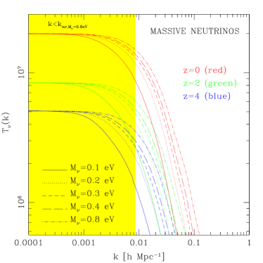
Finally, Figure 3 shows the neutrino linear transfer functions for the same mass and redshift ranges as considered before, with arbitrary normalization.
It is of considerable interest to investigate how these effects propagate in the nonlinear regime, not only at the level of the three-dimensional matter power spectrum, but also for the one-dimensional Ly flux power spectrum: we address these questions in Section 5.
3.2 Particle implementation of massive neutrinos
Implementing massive neutrinos in cosmological -body simulations is a delicate subject. Firstly, neutrinos can be treated either as a fluid or as an ensemble of particles. Secondly, one may describe their evolution with linear theory or perform a full nonlinear treatment; clearly, the second option comes with a series of numerical challenges, in primis the problem of shot noise introduced by the high thermal velocities of the neutrino component.
Several attempts along these lines have already been made in the literature, even long ago (e.g., White, Frenk & Davis 1983; Klypin et al. 1993; Ma & Bertschinger 1994). More recently, Brandbyge et al. (2008) described a simple method for including the effect of massive neutrinos in large-scale -body simulations, using a hybrid TreePM approach, but neglecting all the hydrodynamics; their findings already showed that the suppression of power due to the presence of massive neutrinos is increased by nonlinear effects. Subsequently, Brandbyge & Hannestad (2009) modeled neutrinos as a fluid with a grid method, and pointed out the relative benefits and drawbacks of implementing the effects of neutrinos in the form of particles versus a grid-based implementation. In their code, the gravitational force due to neutrinos is calculated using the linearly evolved density distribution of the neutrinos in Fourier space. Obviously, this technique eliminates the Poisson noise at small scales introduced by an alternative particle representation, which results in higher accuracy in regions where the effect of the nonlinear neutrino evolution is mild. With this approach a series of computational problems are avoided or drastically reduced, such as memory and CPU time consumption – as one does not need to store neutrino positions and velocities. In another study, Brandbyge & Hannestad (2010) combined grid- and particle-based methods with a hybrid technique to achieve good accuracy at small and large scales while keeping the CPU consumption under control: neutrinos are first discretized on a grid, and subsequently part of the grid is converted into -body particles, when the thermal motion of neutrinos decreases to a few times the flow velocities in the simulation. Instead, Ali-Haïmoud & Bird (2013) used a different technique: the CDM component is obtained via -body computations, while the smooth neutrino component is evaluated from that background by solving the Boltzmann equation linearized with respect to the neutrino overdensity.
In the present work, we choose a more direct and computationally intensive approach – following Viel et al. (2010): neutrinos are modeled as an additional type of particle in the -body setup (on top of gas and DM), and a full hydrodynamical treatment is carried out, well-inside the nonlinear regime – including the effects of baryonic physics which affect the IGM. In particular, we make no approximations for the evolution of the neutrino component, nor interchange between grid- and particle-based implementations to save CPU time or speed up the computations. The adopted implementation technique is primarily driven by our main goal to accurately reproduce all the main features of the Ly forest, at the quality level of BOSS or future deep Ly surveys. As evident from Figure 1 (i.e., yellow versus gray areas), the one-dimensional Ly forest data provided by BOSS lies in a -range where nonlinear evolution of cosmological neutrinos cannot be neglected: hence, any attempt to speed-up calculations by using approximate linear solutions for the neutrino component would compromise our ability to accurately reproduce all the features of the forest. To this end, Viel et al. (2010) previously compared particle and grid neutrino representations and found that their difference in terms of power spectra are mainly driven by the fact that the nonlinear evolution at small scales is not properly reproduced by the grid method; they also argued that on scales relevant for the Ly forest it provides higher accuracy to account for the nonlinear evolution rather than limiting the description to the linear case, despite the effect of the Poisson contribution on the neutrino power spectrum introduced by the particle-based modeling. This fact alone would be sufficient to justify our choice of the particle-based implementation for neutrinos. In addition, we are not limited by computational time or memory because we have access to state-of-the-art computational facilities to perform a complete hydrodynamical treatment – as we describe next.
4 OUR SIMULATIONS
In this section we present our new suite of hydrodynamical simulations with massive neutrinos and provide several technical details on the codes used for the runs, the performance, and the various optimization strategies. We also briefly describe the workflow pipeline and the post-processing procedure developed to extract the line of sight (LOS) and particle samples to accurately model the Ly transmitted flux.
4.1 Suite of simulations with massive neutrinos
| Parameter | Value |
|---|---|
| 0.83 | |
| 0.96 | |
| [km s-1Mpc-1] | 67.5 |
| 0.31 | |
| 0.044 | |
| 0.69 | |
| 15000 | |
| 1.3 | |
| Starting redshift | 30 |
| Simulation set | [eV] | Boxes [Mpc/h] | Mean particle separation [Mpc/h] | ||
|---|---|---|---|---|---|
| BG a/b/c | 0 | 0.830 | 100/25/25 | 768/768/192 | 0.1302/0.0325/0.1302 |
| NUBG a/b/c | 0.01 | 0.830 | 100/25/25 | 768/768/192 | 0.1302/0.0325/0.1302 |
| NU01 a/b/c | 0.1 | 0.830 | 100/25/25 | 768/768/192 | 0.1302/0.0325/0.1302 |
| NU01-norm a/b/c | 0.1 | 0.810 | 100/25/25 | 768/768/192 | 0.1302/0.0325/0.1302 |
| NU02 a/b/c | 0.2 | 0.830 | 100/25/25 | 768/768/192 | 0.1302/0.0325/0.1302 |
| NU03 a/b/c | 0.3 | 0.830 | 100/25/25 | 768/768/192 | 0.1302/0.0325/0.1302 |
| NU04 a/b/c | 0.4 | 0.830 | 100/25/25 | 768/768/192 | 0.1302/0.0325/0.1302 |
| NU04-norm a/b/c | 0.4 | 0.733 | 100/25/25 | 768/768/192 | 0.1302/0.0325/0.1302 |
| NU08 a/b/c | 0.8 | 0.830 | 100/25/25 | 768/768/192 | 0.1302/0.0325/0.1302 |
| NU08-norm a/b/c | 0.8 | 0.644 | 100/25/25 | 768/768/192 | 0.1302/0.0325/0.1302 |
| Simulation set | [eV] | Boxes [Mpc/h] | |||||||
|---|---|---|---|---|---|---|---|---|---|
| NU08 a/b/c | 0.8 | 0.83 | 100/25/25 | 768/768/192 | 1.6 | 67.5 | 0.96 | 0.31 | 15000 |
| NU08 a/b/c | 0.8 | 0.83 | 100/25/25 | 768/768/192 | 1.3 | 72.5 | 0.96 | 0.31 | 15000 |
| NU08 a/b/c | 0.8 | 0.83 | 100/25/25 | 768/768/192 | 1.3 | 67.5 | 1.01 | 0.31 | 15000 |
| NU08 a/b/c | 0.8 | 0.83 | 100/25/25 | 768/768/192 | 1.3 | 67.5 | 0.96 | 0.36 | 15000 |
| NU08 a/b/c | 0.8 | 0.88 | 100/25/25 | 768/768/192 | 1.3 | 67.5 | 0.96 | 0.31 | 15000 |
| NU08 a/b/c | 0.8 | 0.83 | 100/25/25 | 768/768/192 | 1.3 | 67.5 | 0.96 | 0.31 | 21000 |
∗ a/b/c indicate the different box size and number of particles in the simulation.
We performed a total of 48 hydrodynamical simulations, both with varying neutrino mass and fixed cosmological and astrophysical parameters (group I), or with a fixed neutrino mass and slight variations in the basic cosmological and astrophysical parameters (group II) around what we indicate as the ‘best-guess’ run – this is the reference simulation set without massive neutrinos (but a massless neutrino component) and a cosmology compatible with the latest Planck (2013) results. The basic parameters common to all the realizations are reported in Table LABEL:tab_param_sims.
For a given neutrino mass, we always performed a set of three simulations with different box sizes and number of particles (their combinations determine the lowest and highest -modes that can be resolved), which are appropriate for the quality of BOSS; specifically, we adopted a box size of for large-scale power with a number of particles per component (simulations ‘a’ in Tables LABEL:tab_suite_sims_A and LABEL:tab_suite_sims_B), and a box size of for small-scale power, in this case with or , respectively (simulations ‘b’ and ‘c’ in Tables LABEL:tab_suite_sims_A and LABEL:tab_suite_sims_B). Extensive convergence and resolution tests in support of our settings have been carried out in Borde et al. (2014) – but see also Section 5.1. In particular, the reason behind our specific choice is the ability to match the sensitivity of the BOSS quasar catalog (Pris et al. 2012) from Data Release 9 (Ahn et al. 2012), and is also related to the application of the splicing technique proposed by McDonald (2003), which allows correcting the larger box size simulation for the lack of resolution and the small box for the lack of nonlinear coupling between the highest and lowest -modes; in this way, we are able to achieve an equivalent resolution of billion particles in a box size – optimal also for eBOSS and DESI – without the need of running a single but computationally prohibitive numerical simulation.
When we included massive neutrinos we always kept fixed to give a flat geometry (with ) and varied the additional massive neutrino component to the detriment of . Moreover, most of our runs were tuned to have at by construction, which is the observed Planck (2013) value. However, to characterize the effect of massive neutrinos with respect to the case of massless neutrinos, we also ran simulations with the initial spectral amplitude fixed as in the best-guess, and therefore with values of changing across redshifts; these additional simulations are termed normalized and are used here to quantify the impact of massive neutrinos on the matter power spectrum; in models with massive neutrinos, the power is suppressed on scales smaller than the free-streaming scale when the normalization is fixed, as explained previously.



Aside from the best-guess run, which only has a massless neutrino component, all our other simulations contain three degenerate species of massive neutrinos implemented as a single particle-type, where , and eV. To ensure that the various realizations correctly converge when , we also ran a simulation set with a very low neutrino mass, i.e. – indicated as NU best-guess (see the appendix for a sanity check test). In addition, we performed a series of realizations with the neutrino mass fixed to be , and slightly varied the basic cosmological and astrophysical parameters around the best-guess reference. Specifically, we considered variations of in the amplitude of the matter power spectrum , in the spectral index of the primordial density fluctuations , and in the matter density content , while we varied the Hubble constant by ; regarding astrophysical parameters, we altered both and , the former by and the latter by . The suite of simulations with best-guess cosmological and astrophysical parameters and varying neutrino mass (group I) – including runs with different normalizations – is summarized in Table LABEL:tab_suite_sims_A; the realizations indicated as neutrino cross-terms (group II), in which we kept the neutrino mass fixed to be but varied cosmology and astrophysics around the best-guess, are listed in Table LABEL:tab_suite_sims_B. To this end, we note that the reason for producing cross-terms is motivated by the multidimensional parameter estimation procedure outlined in Viel et al. (2010); in a forthcoming study, we will apply this technique to constrain cosmological parameters and neutrino masses from the Ly forest by combining results from these simulations and BOSS Ly data.
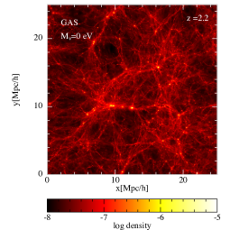
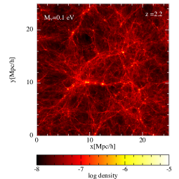
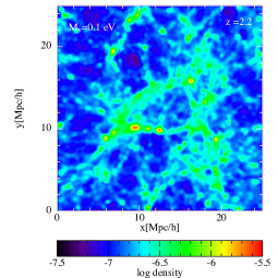
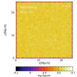
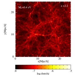
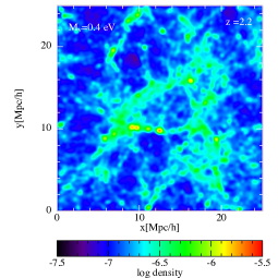
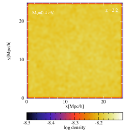
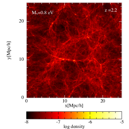
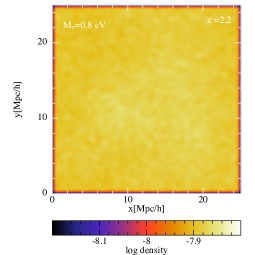
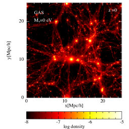
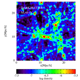
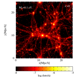
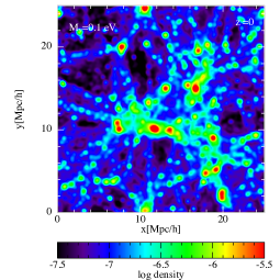
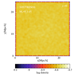
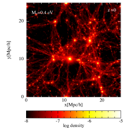
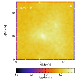
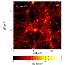
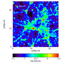
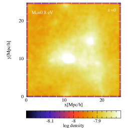
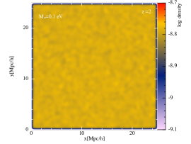
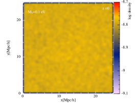
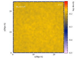
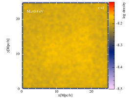
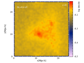
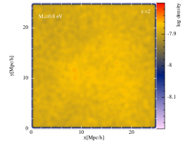
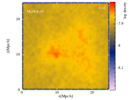
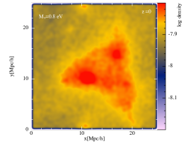
All our runs started at , with initial conditions having the same random seed and based on the second-order Lagrangian perturbation theory (2LPT; Crocce et al. 2006) instead of on the Zel’dovich approximation. Snapshots were produced at regular intervals in redshift between , with ; for a few runs, we also reached . We provide visual examples of our snapshot outputs at and in Figures 4 and 5 for the gas (left panels), dark matter (central panels), and neutrino (right panels) components – when present. The upper top panels are projections of the density field along the and directions (and across ) from our best-guess reference simulation, which only contains massless neutrinos, with a box size of and a relatively low resolution particles per type; in descending order, the other panels are for , and . The axis scales are in . Note that for the neutrino component the density scale is kept fixed only for a given neutrino mass, but changes for different values. The various plots were smoothed with a cubic spline kernel, and both DM and neutrinos were treated like the gas. It is nontrivial to visualize the neutrino component, especially because of shot noise – in essence, for a very small neutrino mass, the overall effect is similar to that of random noise, whereas structures start to appear at increasing and decreasing redshifts.
In all our simulations, the gas was assumed to be of primordial composition with a helium mass fraction of . Metals and evolution of elementary abundances were neglected. As in Viel et al. (2010), we used a simplified criterion for star formation: all gas particles whose overdensity with respect to the mean is above 1000 and whose temperature is lower than K were turned immediately into star particles. This criterion, while having negligible effects on the Ly flux statistics, speeds the calculations up considerably – see Viel et al (2006, 2009), where effects of adopting this simplified strategy were estimated to be about in the Ly statistics, compared with a more elaborate multiphase model.
The various simulations were performed with periodic boundary conditions and an equal number of dark matter, gas, and neutrino particles. We employed the entropy formulation of SPH proposed by Springel & Hernquist (2002). Gas in the simulations was photoionized and heated by a spatially uniform ionizing background. This background was applied in the optically thin limit and was switched on at . The resulting reference thermal history in our simulations is consistent with the recent temperature measurements of Becker et al. (2011), assuming a slope for the temperature-density relation of . We furthermore explored a variety of different thermal histories around this reference, parameterized by and , which allowed us to span a plausible range for these two parameters within the observational uncertainties. We achieved this by rescaling the amplitude and density dependence of the photoionization heating rates in the simulation (e.g. Becker et al. 2011). Details on the software developed for this study are provided next.
4.2 Codes, optimization, and performance
The basic code used for our simulations is Gadget-3 (Springel et al. 2001; Springel 2005), supplemented by CAMB (Lewis, Challinor & Lasenby 2000), and a modified version of 2LPT (Crocce et al. 2006) to determine the initial conditions.
In particular, Gadget-3 (GAlaxies with Dark matter and Gas intEracT) is a massively parallel tree-SPH code for collisionless and gasdynamical cosmological simulations. Gravitational interactions are computed with a hierarchical multipole expansion via the standard -body method, and gas-dynamics is followed with SPH having fully adaptive smoothing lengths, so that energy and entropy are conserved; collisionless DM and gas are both represented by particles. The gravitational force computation uses a hierarchical multipole expansion, optionally in the form of a tree-PM algorithm: short-range forces are treated with the tree method, and long-range forces with Fourier techniques. For our realizations, we set the number of mesh cells of the PM grid equal to the number of particles.
With respect to its original version, Gadget underwent a series of improvements and optimizations over several years to maximize the work-load balance and the efficiency in memory consumption and communication bandwidth. The high-level optimization of the code is obtained via a new parallelization strategy, based on a space decomposition achieved with a space-filling curve (i.e. the Peano-Hilbert decomposition). This fact guarantees a force independent of the processor number.
Several other physical processes have also been implemented in Gadget-3, from radiative cooling/heating physics to nonstandard DM dynamics, star formation, and feedback. However, in our case feedback options were disabled and galactic winds neglected, as suggested by the results of Bolton et al. (2008), who found that winds have a negligible effect on the Ly forest.
Along the lines of Viel et al. (2010), Bird et al. (2012), and Villaescusa-Navarro et al. (2013a,b), Gadget-3 has been modified to simulate the evolution of the neutrino density distribution. In particular, neutrinos are treated as a separate collisionless fluid and are implemented as an additional particle-type on top of gas and DM (see Section 3). To save computational time, the small-scale neutrino clustering is neglected, and their short-range gravitational tree force in the TreePM scheme is not computed. Hence, the spatial resolution for the neutrino component is on order of the grid resolution used for the PM force calculation. We also note that the time-step used by the code is set by the DM alone, and is not affected by the neutrino component.
Lines of sight and particle samples were obtained from Gadget-3 snapshots with an extraction procedure briefly described in the next section; we also developed additional software to handle the post-processing phase. We ran all our parallel codes on the thin nodes of the Curie supercomputer, owned by GENCI and operated in the TGCC by CEA – the first French Tier0 system open to scientists through the French participation in the PRACE research infrastructure.


4.3 Pipeline and post-processing
A typical snapshot from Gadget-3 at a given redshift contains information about positions and velocities for all the components (gas, DM, neutrinos, stars), in addition to specific information about the SPH treatment of the gas (i.e., internal energy, density, hydrogen, and electron fraction and smoothing length). The snapshot goes through an elaborate pipeline to obtain an averaged flux power spectrum and compute the temperature-density relation (cf. eq. 1). To characterize the Ly flux statistics, 10,000 randomly placed simulated quasar sightlines were drawn through the simulation box. Given our largest box size, this implies an average spacing between sightlines of kpc – far smaller than the scale probed by the Ly forest. To generate the flux power spectrum, the absorption due to each SPH particle near the sightline was calculated from the positions, velocities, densities, and temperatures of all the SPH particles at a given redshift – following the procedure described in Theuns et al. (1998) using the SPH formalism; this provides a number of simulated quasar spectra that were smoothed with a three-dimensional cubic spline kernel. As done in Borde et al. (2014), each spectrum was rescaled by a constant so that the mean flux across all spectra and absorption bins matched that observed mean flux at redshift (Miralda-Escudé et al.1996; Kim et al. 2007; Meiksin 2009). In particular, we fixed the photoionization rate by requiring the effective optical depth at each redshift to follow the empirical power law , with and . The normalization was performed a posteriori, since finding and fixing the appropriate photoionization rate a priori for each of the simulations would be more computationally demanding. However, the rescaling of the optical depths is possible and routinely done, because simply changing the intensity of the UV background at a fixed redshift without changing the reionization history does not vary the temperature of the gas for an optically thin IGM in ionization equilibrium; the instantaneous temperature only depends on the spectral shape of the UV background and the gas density. This has been demonstrated analytically (e.g., equation 2.16 in Theuns 2005). The rescaling coefficients, which were determined independently for every redshifts, were found to be between and . On the other hand, changing the reionization history would instead modify the integrated thermal history and hence the amount of Jeans smoothing in the IGM – although the impact of varying the hydrogen reionization history on the Ly forest at is relatively modest (e.g., Viel et al. 2005, 2006, 2009; Becker et al. 2011). After performing the normalization procedure, the mean over all the rescaled spectra was used as the extracted flux power spectrum for the box. Finally, the splicing technique of McDonald (2003) was applied to increase the effective resolution (see also Borde et al. 2014 for more details on the splicing method).
5 FIRST RESULTS
In this section we present the first results from the analysis of our suite of hydrodynamical simulations. In particular, after briefly mentioning convergence and resolution tests and showing a few visualization examples, we compute the three- and one-dimensional matter- and flux-power spectra and characterize the one-dimensional statistics of the Ly transmitted flux in presence of massive neutrinos.


5.1 Convergence and resolution tests
Accurately modeling the Ly flux power spectrum and achieving numerical convergence for the Ly forest is challenging because most of the signal comes from poorly resolved underdense regions. In addition, current data at high redshift are noisier than those at low-, which increases the sample variance in the simulation box. Hence, checks for convergence and resolution are important, and one needs to find an optimal compromise between the box size of the simulation, the total number of particles used in the runs, and the overall CPU consumption. Clearly, convergence requirements will always depend on the physical process under consideration, as well as on the precision of the observational data with which the simulations are compared. To this end, extensive tests on convergence and resolution – along the lines of Theuns et al. (1998), Bryan et al. (1999), Regan, Haehnelt & Viel (2007) and Bolton & Becker (2009) – have been carried out in Borde et al. (2014). Their results have motivated the choices of box sizes and resolutions in this work, and the overall strategy of using a set of three simulations and applying the splicing technique (instead of performing a single but computationally too demanding run), which allows for a substantial decrease of modeling errors because of the improved particle resolution. Given our setting choices, numerical convergence is safely reached; however, since we also added the neutrino component as another type of particle and performed a complete hydrodynamical treatment, our simulation workload was heavier than simpler realizations with only gas and DM by about – when the number of particle per species was kept equal.
In closing this section, we note that while the tests conducted in Borde et al. (2014) did not consider massive neutrinos, their stringent results about convergence and resolution requirements are readily applicable to our case. This is simply because including massive neutrinos is essentially equivalent (with very minor effects, at least in terms of convergence and resolution) to a neutrino-less situation with a slightly different value of the parameter – see for example Viel et al. (2010), where the degeneracy is discussed in some detail. In addition, observational uncertainties on the BOSS power spectrum are at a level that is less stringent than the requirements imposed in Borde et al. (2014).
Regarding the splicing technique, neutrinos are expected to introduce a smooth suppression in terms of matter power spectrum, and the splicing technique is able to capture this effect in the range of redshifts and wavenumbers we are interested in. In fact, the splicing technique can detect smooth variations of amplitude in matter power across the scales (although, very likely, this will no longer be the case for warm dark matter where the induced suppression is abrupt and stronger than in the neutrino case).
5.2 Visualizations
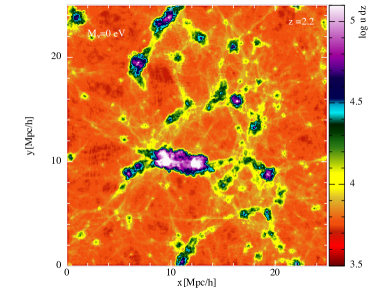
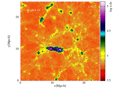
Massive neutrinos induce changes in the thermal state of the gas and in the LSS clustering of DM. Differences are even visually perceptable for relatively large neutrino masses, for example, in the distribution of the internal energy of the gas (and hence of its temperature), when compared with simulations with massless neutrinos. Figure 6 provides an example: in the various panels, we show a slice of the internal energy of the gas from simulation snapshots at , when the box size is and the resolution is /type; the upper left panel is from a simulation with massless neutrinos, and in clockwise direction the values of the neutrino mass increase as , and eV. Changes in the thermal state of the gas are particularly relevant for the power-law relation (cf. eq. 1), which is thought to arise from the competition between photoheating and cooling due to the adiabatic expansion of the Universe, following reionization. The evolution of this relation has been measured in the data and depends on the reionization history and the hardness of the UV background (Schaye et al. 2000; Ricotti et al. 2000; McDonald et al. 2001; Rollinde et al. 2013), although in reality the picture is more complicated – because of radiative transfer effects during the epoch of HeII reionization. Nevertheless, the temperature at the characteristic overdensity probed by the Ly is now quite well measured (e.g. Becker et al. 2011). The main uncertainty that remains is the slope () of the relation: this is still poorly measured and translates into an uncertainty on (at mean density). Hence, a more accurate modeling of the thermal state of the gas is required to reduce uncertainties in the thermal state of the IGM – when massive neutrinos are also present.
Figure 7 shows the density evolution of the neutrino component from simulations with box sizes and resolution /type, at (left panels), (central panels), and (right panels) as a function of the neutrino mass; top panels show eV, intermediate panels represent eV, and the bottom panels eV. The axis scales are in . Note again that for the neutrino component the density scale is kept fixed only for a given neutrino mass, while it changes across different values. The distribution of the neutrino density has been smoothed with a cubic spline kernel to eliminate spurious Poisson noise at the smallest scales to obtain genuine cosmological density fluctuations of the neutrinos that occur only on large scales – because of their free-streaming. According to Viel et al. (2010), typical neutrino fluctuations at the largest scales are about around the mean, while for gas and DM the fluctuations are usually much stronger. Moreover, the growth of structures is less evolved in the simulation with neutrinos (i.e., the voids are less empty) since their suppressed clustering slows down the growth of the perturbations in the overall matter density, and this in turn affects the properties of the gas and DM.
Clearly, one of the main consequences of the particle-based implementation of massive neutrinos is the presence of shot noise. To this end, Viel et al. (2010) have conducted an extensive computation of shot noise (see their Section 3.4 and their Figures 9 and 17) and considered the effect of varying the number of neutrino particles both on the matter and flux power spectra. Their findings suggest that doubling the neutrino particles for each spatial dimension shifts the Poisson contribution to the matter power spectrum by a factor of roughly two to smaller scales. Hence, it would be desirable for Ly studies to increase the number of neutrino particles to decrease the Poisson contribution to the matter power spectrum and sample the neutrino power spectrum properly on scales between 0.1 and 2 . However, Viel et al. (2010) also pointed out that increasing the number of neutrino particles by a factor of eight can be done but required a factor of more in CPU time. Therefore, one has to balance the demand in terms of parallel computing resources with the desired resolution. Fortunately, although the neutrino power spectrum is affected by shot noise at the smallest scales, the impact on the matter power spectrum, and thus on the one-dimensional flux power spectrum (which is the main quantity we are after), is still very small because the neutrinos constitute a very small fraction of the overall matter density. Hence, in our regime of interest – which is analogous to that of Viel et al. (2010) – a single neutrino particle per CDM particle is sufficient.
5.3 Three-dimensional matter power spectra
Next, we consider the set of neutrino simulations with particles per type and a box size of Mpc, with the same spectral amplitude as the corresponding best-guess run (i.e., the normalized simulations). Values of at for these realizations are provided in Table LABEL:tab_suite_sims_A. From these runs, we compute the three-dimensional total matter power spectra and compare results with linear predictions.
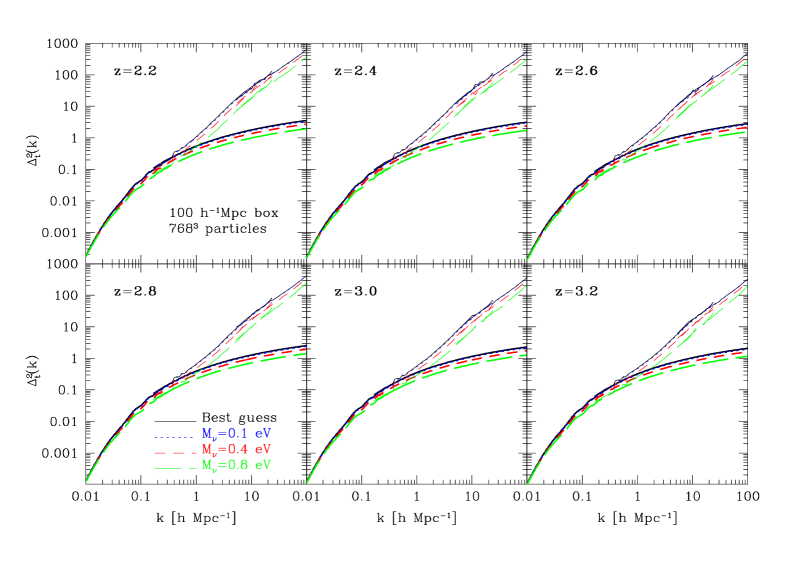
In Figure 8, we show results of this comparison. Black lines denote the best-guess realization, and dotted, dashed, and long-dashed lines are used for runs with massive neutrinos with , and eV. Six intervals in redshifts were considered, from to , with a spacing . The linear evolution (thick lines) was computed from CAMB as explained in Section 3, while the nonlinear power spectra (thin lines) were obtained from Gadget-3 snapshots. As can be directly inferred from the various panels, the free-streaming of neutrinos results in a suppression of the power spectrum of the total matter distribution at scales probed by the Ly forest data, which is higher than the linear theory prediction by about () at scales when eV ( eV) and is strongly redshift dependent. The effects of free-streaming of neutrinos on the matter power spectrum have been discussed in detail in Viel et al. (2010): we here confirm their findings of a mass- and redshift-dependence suppression of the power spectrum at small scales, which is more significant with increasing neutrino mass. At large scales, linear and nonlinear evolution in the power spectrum are similar, as already pointed out in Figure 1, where we argued that a linear description for the neutrino component is sufficient inside the yellow area (when ).
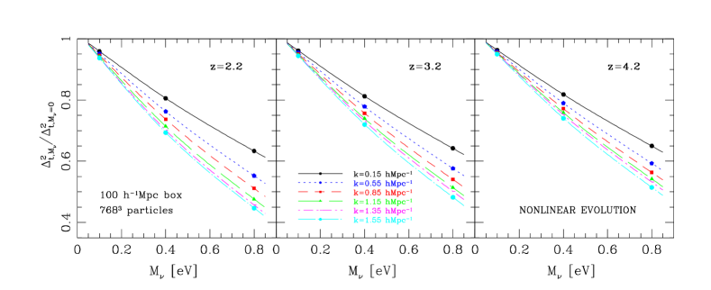
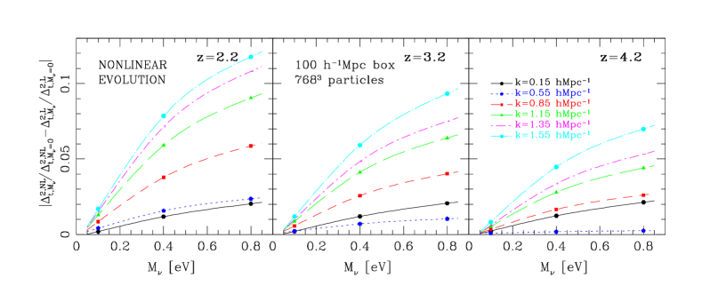
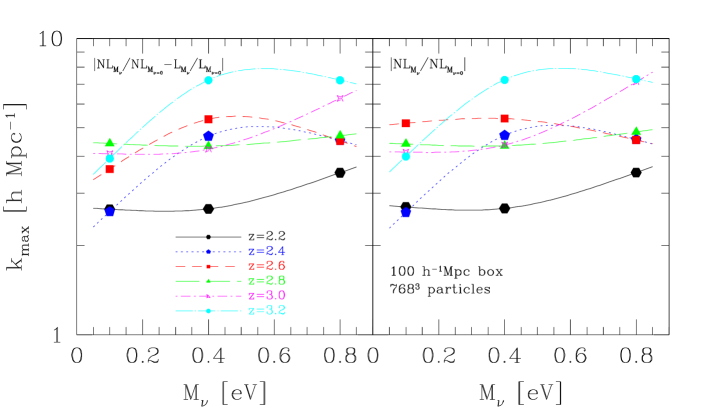
Figure 9 shows all these effects more clearly: as a function of , we plot the total three-dimensional matter power spectra in presence of massive neutrinos, normalized by their corresponding power spectra from neutrino massless simulations at the same resolution. The top panel shows , the middle panel , and the bottom panel . In the panels, the almost straight lines are linear theory expectations: the plateau of nearly -independent suppression predicted by linear theory is approximately described by and depends only very weakly on redshift. Clearly, the inclusion of nonlinear effects produces a characteristic -dependent suppression (i.e., the dips in the figure) on the three-dimensional matter power spectrum, which varies as a function of mass; the higher the value of , the higher the -mode where the dip occurs. Similarly, for a given neutrino mass, at increasing redshifts the position of the maximum suppression deep is altered in a nontrivial way – but typically toward smaller scales. The trend we find here appears to be consistent with analogous results in Bird et al. (2012). Note also that there is an upturn in the suppression, which was first reported and briefly discussed in Brandbyge et al. (2010), and was investigated in depth in Viel et al. (2010). In particular, according to Viel et al. (2012), it appears to be related to the nonlinear collapse of halos decoupling from the large-scale modes slightly differently in simulations with massive neutrinos than in simulations with only massless neutrinos, and has been shown by the same authors not to depend on the number of neutrino particles – ruling out shot noise as a plausible cause. This finding suggests that virialization of halos is slightly modified by the smoothly distributed neutrino component, in a similar way as by dark energy where this is a well-known effect (Alimi et al. 2010).
In the top panels of Figure 10 we study these effects in depth by displaying the total nonlinear matter power spectra in simulations with massive neutrinos, normalized by the case with only a massless neutrino component, but now as a function of neutrino mass () and for different values of in the range relevant for the one-dimensional BOSS Ly forest data. Specifically, we assumed , and with different line styles, for three different redshift slices (from left to right, , and ). For a given redshift interval, the detected trend at increasing is essentially linear, as expected from Figure 9, with departures from the best-guess simulations, which are more significant at lower redshift and for a larger neutrino mass.
Is of more interest to consider the evolution of the quantity defined by
| (8) |
namely the difference between nonlinear and linear 3D power spectrum predictions, expressed in terms of ratios (as defined before). This is shown in the bottom panels of Figure 10 for the same redshift intervals and -values as considered in the top panels. Spline fits are used to connect points with the same -value. Clearly, at increasing redshift departures from linear theory are less significant, particularly for smaller neutrino masses and lower values of . Within the Ly range of interest, it is clear that is maximized at lower and higher values of .
Finally, in the left panel of Figure 11 we find the value of for which the quantity (i.e., the difference between linear and nonlinear evolution in terms of ratios) is maximized – without restricting the wavenumber to the BOSS Ly range. Spline fits are again used to connect points with the same and different values of the neutrino mass. This plot is particularly useful because at a given redshift it provides a quick way to determine at which there is more sensitivity to the neutrino mass, meaning that it shows where the effects due to neutrino free-streaming are more pronounced. The right panel of the same figure shows analogous information, but now determined by considering the nonlinear evolution alone. Since the power suppression caused by neutrinos is essentially constant at scales (Lesgourgues & Pastor 2006), using either the normalized differences between linear and nonlinear evolution (i.e., the quantity previously defined), or just the one given by the nonlinear evolution of the neutrino component in terms of the massless neutrino case should not make a significant difference; this is in fact confirmed in the right panel of Figure 11. The nonlinear power spectrum strongly depends on redshift and the dependence of scale becomes steeper with decreasing redshift. It is interesting to see how these effects propagate into the Ly flux power spectrum: we briefly discuss this in the next section and treat the one-dimensional statistics in depth in a forthcoming publication.
Before moving on, we note that there are several other numerical effects that can potentially impact the power spectrum: the number of neutrino particles, the velocities in the initial conditions, the sampling of the initial conditions with neutrino pairs to balance momentum, and the starting redhsift. All these effects have been investigated in Viel et al. (2010) and are not further discussed here.
5.4 One-dimensional analysis: flux statistics
The effect of neutrino free-streaming is a small scale-dependent suppression of the total matter power, which is a function of redshift and mass of the neutrinos. In this part, we briefly address how this signal affects the statistical properties of the transmitted flux fraction (the main observable along a number of quasar sightlines). The Ly transmitted flux , treated as a continuous field, is defined as
| (9) |
where is the optical depth; the corresponding flux fraction power spectrum is
| (10) |
where - 1. Here is the mean flux and the tilde symbol denotes a Fourier-transformed quantity. The calibration of the mean flux level is the main systematic error, along with uncertainties in the thermal history of the IGM, and the different scaling given by different simulations. The mean flux, a measure of the average density of neutral hydrogen, has a stong impact on the amplitude of the flux power spectrum (Viel et al. 2010).
Below, we mostly focus on the flux power spectrum, although one can explore the flux statistics with a variety of tools such as the flux PDF and the flux bispectrum (see for example Mandelbaum et al. 2003; Viel et al. 2004; Fang & White 2004; Lidz et al. 2006; Bolton, Oh & Furlanetto 2009; McQuinn et al. 2009; Viel et al. 2009).
The flux power spectrum of the Ly forest is sensitive to a wide range of cosmological and astrophysical parameters and instrumental effects and has been extensively used in the literature as a probe of the primordial matter power spectrum on scales of Mpc at ; it does not have a simple algebraic relationship to the matter power spectrum because of nonlinearities in the flux-density relation. Note in fact that by the most important absorbing structures are weakly nonlinear. The Ly flux distribution depends on the spatial distribution, the peculiar velocity field, and the thermal properties of the gas. Going from the observed flux distribution to the power spectrum of matter in LSS requires knowledge of the bias of gas to matter, which in turns demands the temperature-density relation of the gas and its evolution over cosmic history, as well as the nature of the ionizing background radiation. Hence, the only way to compute it is to rely on hydrodynamical simulations. The flux power spectrum can also be used to constrain cosmological parameters and the nature of dark matter through its shape and redshift dependence (Croft et al. 2002). In addition, the Ly forest power spectrum at small scales allows much improved constraints on the inflationary spectral index the running of that index with scale, and neutrino masses.
The relation between the three- and one-dimensional power spectra is given by
| (11) |
and in linear theory one has with , the density bias and the redshift distortion parameter. As anticipated, one can rely on accurate high-resolution and large box-size hydrodynamical simulations to model the bias function , which relates the flux to the linear dark matter power spectrum: .
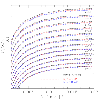
Figure 12 shows an example of the one-dimensional flux power spectra computed from our simulation sets (BG, NU04, NU08), without (solid) and with (dotted and dashed) massive neutrinos – after application of the splicing technique. In particular, we considered two neutrino masses, namely and eV. Note that here the wave vector is measured in (km/s)-1. To perform our analysis, we extracted 10,000 mock quasar absorption spectra from the simulation sets at various redshift intervals – from with . The optical depth was rescaled in the standard way to match the observed effective optical depth at , as given by Schaye et al. (2003), that is, , and to reproduce the same mean flux level; this procedure is justified because the HI photoionization rate adopted in the simulations is inversely proportional to the Ly optical depth in our mock spectra – see Viel et al. (2010) for more details.
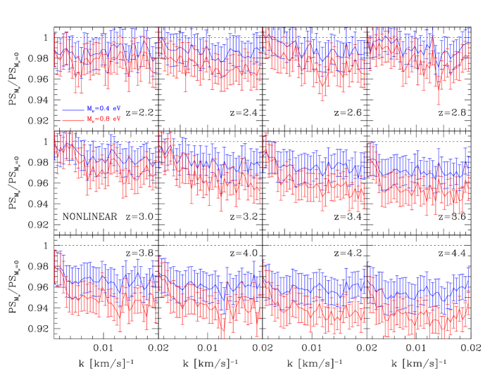
Figure 13 displays similar quantities as the previous figure, but now the flux power spectra are normalized by the corresponding measurements obtained from simulations with massless neutrinos. Error bars are estimates derived from 10,000 LOS. As in Viel et al. (2010), we also compared simulations with massive neutrinos against those with only a massless neutrino component and a reduced overall amplitude of the matter power spectrum. This allows distinguishing the effect of the neutrino free-streaming on the shape of the flux power spectrum and its evolution from the overall suppression of power due to the free-streaming. The latter is responsible for the well-known degeneracy between neutrino mass and . In essence, the differences in the matter power spectra translate into a difference in the flux power spectrum for neutrino masses with eV, which varies with redshift and is more pronounced at – if simulations are normalized to have the same in the initial conditions. This very weak effect is difficult to detect from present Ly data and, according to Viel et al. (2010), nearly perfectly degenerates with the overall amplitude of the matter power spectrum . As in Viel et al. (2010), we found that the overall suppression of power induced by massive neutrinos on the flux power spectrum becomes stronger with larger neutrino mass and at higher redshift values, while there is an upturn and a bump at smaller scales.
In closing, we note that all our comparisons between simulations with massive neutrinos and with only a massless neutrino component were made assuming the same initial random seed for both simulations, so that the contribution from cosmic variance is effectively removed. The reason behind our choice, following Viel et al. (2010), is that we aim at distinguishing the effect of a varying neutrino mass from the additional complication introduced by cosmic variance. Namely, in this work we are more concerned about quantifying the impact of changing neutrino masses and how this translates both into the total matter power spectrum and into the flux power spectrum – separating this latter effect from the contribution caused by cosmic variance. However, when simulations are used to compare with data, it is important to quantify the effect of cosmic variance – as done for example in Borde et al. (2014) to contrast simulation results with BOSS data (see their Section 6.1, and their Table 5). To this end, we ran simulations with two different initial random seeds to show the order of magnitude of the cosmic variance effect and where the difference mostly resides: as expected, the derived power spectra for the two seeds agree excellently well at small scales, while at larger scales they can differ up to 2 to 3 at all redshifts because of cosmic variance. Therefore, at large scales cosmic variance has an impact on the power spectrum that exceeds the simulation statistical uncertainty and needs to be included as a systematic uncertainty when applying our model to data.
6 CONCLUSIONS
The determination of the neutrino mass and the nature of the neutrino mass hierarchy are key issues in particle physics today – directly connected with the origin of mass. To this end, cosmology offers the best sensitivity to the neutrino mass, and by combining cosmological and particle physics results from solar, atmospheric, reactor, and accelerator observations of neutrino oscillations the absolute mass scale of neutrinos can probably be determined in the very near future.
Massive neutrinos impact the CMB power spectrum and affect the LSS – depending on the epoch at which they have become non-relativistic. Because of their free-streaming, they also alter the low- power spectrum and lead to a modified redshift-distance relation. In essence, neutrinos suppress power in DM clustering on small scales, which erases their own fluctuations on scales below the free streaming length. In turn, this slows down the growth of CDM structure on the same scale, leaving an imprint on the matter power spectrum. The overall result is a model of the Universe different from the standard CDM scenario, with important consequences on the structure formation mechanism.
Typically, limits on neutrino masses from cosmology are directly obtained from the analysis of the CMB radiation via the CMB power spectrum, the ISW effect on polarization maps, or through gravitational lensing of the CMB by LSS. Other popular methods for quantifying the impact of massive neutrinos are based on galaxy clustering and exploit high-redshift surveys. On the other hand, fewer studies involve the Ly forest, which is now emerging as a unique window into the high-redshift Universe, because it is located at a redshift range inaccessible to other LSS probes and spans a wide interval in redshift. The Ly forest is a powerful tool for constraining neutrino masses, since massive neutrinos impact the one-dimensional flux power spectrum, because they suppress the growth of cosmological structures on scales smaller than the neutrino free-streaming distance. For neutrino masses below eV, the full extent of the suppression occurs on megaparsecs scales. In addition, combined with CMB observations and other tracers sensitive to large scales, the power spectrum of the Ly forest can provide stringent constraints on the shape and amplitude of the primordial power spectrum, and hence directly test models of inflation (Viel et al. 2005; Seljak et al. 2005; Viel & Haehnelt 2006).
Therefore, a detailed modeling of the line-of-sight power spectrum of the transmitted flux in the Ly forest with massive neutrinos is required. The main goal of our study was indeed to provide a novel suite of state-of-the-art hydrodynamical simulations with cold dark matter, baryons, and massive neutrinos, targeted at modeling the low-density regions of the IGM as probed by the Ly forest at high redshift. Our simulations spanned volumes ranging from to , and were made using either million or billion particles – with chosen cosmological parameters compatible with the latest Planck (2013) results.
As explained in Section 3, neutrinos were implemented as a new type of particle in the -body setup (on top of gas and DM), and we considered three degenerate species with masses , and eV. This more direct and computationally intensive approach is primarily driven by our goal to accurately reproduce all the main features of the Ly forest at the quality level of BOSS or future deep Ly surveys. Figure 1 shows that the one-dimensional Ly forest data provided by BOSS lies in a -range where nonlinear evolution of cosmological neutrinos cannot be neglected, and hence any attempt to speed-up calculations by using approximated linear solutions for the neutrino component – instead of a full hydrodynamical treatment – would compromise our ability to reproduce accurately all the features of the forest.
Technical aspects of the new suite of hydrodynamical simulations, such as details on the code used for the runs, initial conditions, optimization strategies and performance, along with various improvements and a description of the pipeline developed to extract the synthetic Ly transmitted flux, were presented in Section 4 – building upon the theoretical background of Sections 2 and 3 (see also Tables LABEL:tab_suite_sims_A and LABEL:tab_suite_sims_B). Since we are planning to make the simulations available to the scientific community upon request, this part may be regarded as a guide for a direct use of the simulations.
We improved on previous studies in several directions, in particular with updated routines for IGM radiative cooling and heating processes, and initial conditions based on 2LPT instead of on Zel’dovich approximation. Figures 4 and 5 are visual examples of a few snapshots at and for the gas, dark matter, and neutrino components – when present – in a simulation with particles per type and a box size of Mpc.
Using the splicing technique introduced by McDonald (2003), the resolution of our runs can be further enhanced to reach the equivalent of billion particles in a box size. This means that our simulations, specifically designed to meet the requirements of the BOSS survey (which has already identified QSO over square degrees within ), are also useful for upcoming or future experiments – such as eBOSS and DESI. In particular, the comoving volume of eBOSS will be nearly ten times that probed by the BOSS galaxy survey, while DESI will exceed BOSS and eBOSS both in volume and in quasar density, increasing the total number of Ly quasars by about a factor of 5.
In addition to providing technical details, in Section 5 we also performed a first analysis of our simulations; in particular, we characterized the nonlinear three- and one-dimensional matter and flux power spectra and the statistics of the transmitted flux in the Ly forest with massive neutrinos. Massive neutrinos induce changes in the LSS clustering of DM and thermal state of the gas (as evident from Figure 6), affecting the relation (equation 1). In Section 5.3, we investigated in more depth the effect of massive neutrinos on the three-dimensional matter power spectrum, where linear and nonlinear evolutions at different redshifts and for various neutrino masses are studied (Figures 8-11). The characteristic redshift- and mass-dependent suppression of the matter power spectrum caused by the massive neutrino component is clearly seen in Figure 9, and the values of most sensitive to the neutrino mass (i.e. the most relevant scales for detecting the power spectrum suppression due to neutrinos) are shown in Figure 11. Finally, we briefly discussed how this feature propagates in the one-dimensional flux power spectrum (Section 5.4, Figures 12 and 13) and affects the statistical properties of the transmitted flux fraction.
This work represents the first of a series of papers dedicated to quantify the effects of massive neutrinos in the Ly forest across different redshift slices and at nonlinear scales. In particular, our primary next goal is to combine the Ly one-dimensional power spectra at different redshifts obtained from these simulations with analogous measurements derived from the BOSS Ly forest data to constrain the sum of the masses of the three neutrino flavors and the main cosmological parameters with improved sensitivity. This is possible via a multidimensional likelihood analysis, a method pioneered by Croft et al. (1998, 2002) and used by Viel & Haehnelt (2006) on SDSS data, or more recently by Palanque-Delabrouille et al. (2013) on SDSS-III/BOSS DR9 quasar spectra. Clearly, at a later stage we will combine our Ly measurements with Planck data and other available datasets (galaxy PS and BAO from BOSS, lensing PS) to derive tighter joint constraints on cosmological and astrophysical parameters, and on the neutrino mass.
In addition, our simulations can be useful for a broader variety of cosmological and astrophysical applications, ranging from the three-dimensional modeling of the Ly forest to cross-correlations between different probes, the study of dark energy and expansion history of the Universe in presence of massive neutrinos, and particle-physics-related topics. Examples include cross-correlation studies along the lines of Font-Ribera et al. (2013), synergies between ground and space missions in constraining the neutrino mass (we note that DESI, DES, LSST, Euclid, and CMB-stage 4 experiments will unambiguously detect the neutrino mass under both hierarchy scenarios), comparison of our results with different hydrodynamical codes and neutrino implementations, and studies of systematics affecting the Ly forest as a tracer. To this end, UV fluctuations at , galactic winds, metal enrichment, re-ionization history, and the thermal history of IGM are all still major uncertainties in any analysis of the Ly forest flux statistics, along with instrument performance and survey design, and they deserve a closer scrutiny.
The full suite of simulations presented in this paper will be made available to the scientific community upon request.
ACKNOWLEDGMENTS
We acknowledge PRACE for awarding us access to resource Curie-thin nodes based in France at TGCC, for our project 2012071264. This work was granted access to the HPC resources of CCRT under the allocation 2013-t2013047004 made by GENCI (Grand Equipement National de Calcul Intensif). A.B., N.P.-D., G.R. and Ch.Y. acknowledge support from grant ANR-11-JS04-011-01 of Agence Nationale de la Recherche. The work of G.R. is also supported by the faculty research fund of Sejong University in 2014. M.V. is supported by ERC-StG ”CosmoIGM”. JSB acknowledges the support of a Royal Society University Research Fellowship. We thank Volker Springel for making Gadget-3 available.
Appendix A A SANITY CHECK
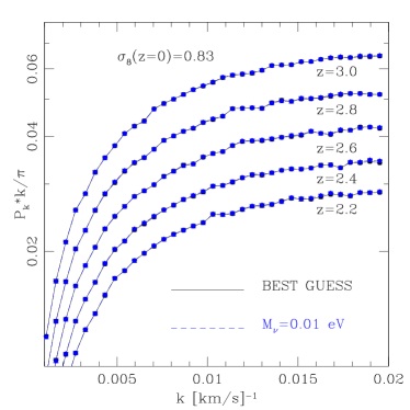
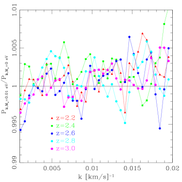
As discussed in Section 5.1, achieving numerical convergence in the modeling of the Ly flux power spectrum is nontrivial. In addition, when we include massive neutrinos in hydrodynamical simulations, the -body setup is quite different from the case of gas and DM alone, since we are dealing with an additional type of particle. Clearly, for a very low value of the neutrino mass, we expect results to be consistent with the case of massless neutrinos. To check that we indeed correctly recover the limit of massless neutrinos, we ran a set of simulations with a very small neutrino mass, eV (i.e., simulation set NUBG a,b,c, in Table LABEL:tab_suite_sims_A). We then extracted the line-of-sight flux power spectra at different redshifts, as done in Section 5.4, and computed their average values across 10,000 random lines. These measurements were compared with analogous measurements obtained from the best-guess run, which did not include massive neutrinos. Results are shown in Figure 14, where it can be seen that convergence is safely achieved in the range of interest.
References
- Abazajian et al. (2005) Abazajian, K., Switzer, E. R., Dodelson, S., Heitmann, K., & Habib, S. 2005, Phys. Rev. D, 71, 043507
- Abazajian & Dodelson (2003) Abazajian, K., & Dodelson, S. 2003, Physical Review Letters, 91, 041301
- Planck Collaboration et al. (2013) Planck Collaboration, Ade, P. A. R., Aghanim, N., et al. 2013, arXiv:1303.5076
- Ahn et al. (2012) Ahn, C. P., Alexandroff, R., Allende Prieto, C., et al. 2012, ApJS, 203, 21
- Ali-Haïmoud & Bird (2013) Ali-Haïmoud, Y., & Bird, S. 2013, MNRAS, 428, 3375
- Alimi et al. (2010) Alimi, J.-M., Füzfa, A., Boucher, V., et al. 2010, MNRAS, 401, 775
- Aracil et al. (2004) Aracil, B., Petitjean, P., Pichon, C., & Bergeron, J. 2004, A&A, 419, 811
- Bahcall & Salpeter (1965) Bahcall, J. N., & Salpeter, E. E. 1965, ApJ, 142, 1677
- Balian & Schaeffer (1989) Balian, R., & Schaeffer, R. 1989, A&A, 220, 1
- Battye & Moss (2013) Battye, R. A., & Moss, A. 2013, arXiv:1308.5870
- Becker et al. (2011) Becker, G. D., Bolton, J. S., Haehnelt, M. G., & Sargent, W. L. W. 2011, MNRAS, 410, 1096
- Bernardeau & Schaeffer (1999) Bernardeau, F., & Schaeffer, R. 1999, A&A, 349, 697
- Bernardeau & Schaeffer (1992) Bernardeau, F., & Schaeffer, R. 1992, A&A, 255, 1
- Bennett et al. (2013) Bennett, C. L., Larson, D., Weiland, J. L., et al. 2013, ApJS, 208, 20
- Bi (1993) Bi, H. 1993, ApJ, 405, 479
- Bi & Davidsen (1997) Bi, H., & Davidsen, A. F. 1997, ApJ, 479, 523
- Bi et al. (1995) Bi, H., Ge, J., & Fang, L.-Z. 1995, ApJ, 452, 90
- Bird et al. (2012) Bird, S., Viel, M., & Haehnelt, M. G. 2012, MNRAS, 420, 2551
- Blake et al. (2012) Blake, C., Brough, S., Colless, M., et al. 2012, MNRAS, 425, 405
- Bolton & Becker (2009) Bolton, J. S., & Becker, G. D. 2009, MNRAS, 398, L26
- Bolton et al. (2009) Bolton, J. S., Oh, S. P., & Furlanetto, S. R. 2009, MNRAS, 395, 736
- Bolton et al. (2008) Bolton, J. S., Viel, M., Kim, T.-S., Haehnelt, M. G., & Carswell, R. F. 2008, MNRAS, 386, 1131
- Bolton & Haehnelt (2007) Bolton, J. S., & Haehnelt, M. G. 2007, MNRAS, 382, 325
- Bond et al. (1980) Bond, J. R., Efstathiou, G., & Silk, J. 1980, Physical Review Letters, 45, 1980
- Borde et al. (2014) Borde, A., Palanque-Delabrouille, N., Rossi, G., et al. 2014, arXiv:1401.6472
- Bouchet et al. (1993) Bouchet, F. R., Strauss, M. A., Davis, M., et al. 1993, ApJ, 417, 36
- Brandbyge & Hannestad (2010) Brandbyge, J., & Hannestad, S. 2010, J. Cosmology Astropart. Phys., 1, 21
- Brandbyge & Hannestad (2009) Brandbyge, J., & Hannestad, S. 2009, J. Cosmology Astropart. Phys., 5, 2
- Brandbyge et al. (2008) Brandbyge, J., Hannestad, S., Haugbølle, T., & Thomsen, B. 2008, J. Cosmology Astropart. Phys., 8, 20
- Bryan et al. (1999) Bryan, G. L., Machacek, M., Anninos, P., & Norman, M. L. 1999, ApJ, 517, 13
- Busca et al. (2013) Busca, N. G., Delubac, T., Rich, J., et al. 2013, A&A, 552, A96
- Carbone et al. (2012) Carbone, C., Fedeli, C., Moscardini, L., & Cimatti, A. 2012, J. Cosmology Astropart. Phys., 3, 23
- Cen et al. (1994) Cen, R., Miralda-Escudé, J., Ostriker, J. P., & Rauch, M. 1994, ApJ, 437, L9
- Crain et al. (2009) Crain, R. A., Theuns, T., Dalla Vecchia, C., et al. 2009, MNRAS, 399, 1773
- Crocce et al. (2006) Crocce, M., Pueblas, S., & Scoccimarro, R. 2006, MNRAS, 373, 369
- Croft et al. (2002) Croft, R. A. C., Weinberg, D. H., Bolte, M., et al. 2002, ApJ, 581, 20
- Croft et al. (1999) Croft, R. A. C., Weinberg, D. H., Pettini, M., Hernquist, L., & Katz, N. 1999, ApJ, 520, 1
- Croft et al. (1998) Croft, R. A. C., Weinberg, D. H., Katz, N., & Hernquist, L. 1998, ApJ, 495, 44
- Coles & Jones (1991) Coles, P., & Jones, B. 1991, MNRAS, 248, 1
- Comparat et al. (2013) Comparat, J., Kneib, J.-P., Escoffier, S., et al. 2013, MNRAS, 428, 1498
- Connolly et al. (2013) Connolly, A., Habib, S., Szalay, A., et al. 2013, arXiv:1311.2841
- Cowie et al. (1995) Cowie, L. L., Songaila, A., Kim, T.-S., & Hu, E. M. 1995, AJ, 109, 1522
- Dawson et al. (2013) Dawson, K. S., Schlegel, D. J., Ahn, C. P., et al. 2013, AJ, 145, 10
- Dodelson et al. (1996) Dodelson, S., Gates, E., & Stebbins, A. 1996, ApJ, 467, 10
- Doroshkevich & Shandarin (1977) Doroshkevich, A. G., & Shandarin, S. F. 1977, MNRAS, 179, 9
- Drinkwater et al. (2010) Drinkwater, M. J., Jurek, R. J., Blake, C., et al. 2010, MNRAS, 401, 1429
- Eisenstein et al. (2011) Eisenstein, D. J., Weinberg, D. H., Agol, E., et al. 2011, AJ, 142, 72
- Fang & White (2004) Fang, T., & White, M. 2004, ApJ, 606, L9
- Font-Ribera et al. (2013) Font-Ribera, A., Kirkby, D., Busca, N., et al. 2013, arXiv:1311.1767
- Fukugita et al. (1998) Fukugita, M., Hogan, C. J., & Peebles, P. J. E. 1998, ApJ, 503, 518
- Gingold & Monaghan (1977) Gingold, R. A., & Monaghan, J. J. 1977, MNRAS, 181, 375
- Gnedin & Hamilton (2002) Gnedin, N. Y., & Hamilton, A. J. S. 2002, MNRAS, 334, 107
- Gnedin & Hui (1998) Gnedin, N. Y., & Hui, L. 1998, MNRAS, 296, 44
- Gnedin & Hui (1996) Gnedin, N. Y., & Hui, L. 1996, ApJ, 472, L73
- Gunn & Peterson (1965) Gunn, J. E., & Peterson, B. A. 1965, ApJ, 142, 1633
- Hamilton (1985) Hamilton, D. 1985, ApJ, 297, 371
- Hannestad (2005) Hannestad, S. 2005, J. Cosmology Astropart. Phys., 2, 11
- Hernquist et al. (1996) Hernquist, L., Katz, N., Weinberg, D. H., & Miralda-Escudé, J. 1996, ApJ, 457, L51
- Hinshaw et al. (2013) Hinshaw, G., Larson, D., Komatsu, E., et al. 2013, ApJS, 208, 19
- Hou et al. (2012) Hou, Z., Reichardt, C. L., Story, K. T., et al. 2012, arXiv:1212.6267
- Hu & Dodelson (2002) Hu, W., & Dodelson, S. 2002, ARA&A, 40, 171
- Hu et al. (1998) Hu, W., Eisenstein, D. J., & Tegmark, M. 1998, Physical Review Letters, 80, 5255
- Hui et al. (2001) Hui, L., Burles, S., Seljak, U., et al. 2001, ApJ, 552, 15
- Hui & Gnedin (1997) Hui, L., & Gnedin, N. Y. 1997, MNRAS, 292, 27
- Hui et al. (1997) Hui, L., Gnedin, N. Y., & Zhang, Y. 1997, ApJ, 486, 599
- Jain & Seljak (1997) Jain, B., & Seljak, U. 1997, ApJ, 484, 560
- Jenkins & Ostriker (1991) Jenkins, E. B., & Ostriker, J. P. 1991, ApJ, 376, 33
- Jones et al. (2009) Jones, D. H., Read, M. A., Saunders, W., et al. 2009, MNRAS, 399, 683
- Kaiser (1992) Kaiser, N. 1992, ApJ, 388, 272
- Katz et al. (1996) Katz, N., Weinberg, D. H., & Hernquist, L. 1996, ApJS, 105, 19
- Kim & Croft (2008) Kim, Y.-R., & Croft, R. A. C. 2008, MNRAS, 387, 377
- Kim et al. (2007) Kim, T.-S., Bolton, J. S., Viel, M., Haehnelt, M. G., & Carswell, R. F. 2007, MNRAS, 382, 1657
- Klypin et al. (1993) Klypin, A., Holtzman, J., Primack, J., & Regos, E. 1993, ApJ, 416, 1
- Kofman et al. (1994) Kofman, L., Bertschinger, E., Gelb, J. M., Nusser, A., & Dekel, A. 1994, ApJ, 420, 44
- Lesgourgues & Pastor (2012) Lesgourgues, J., & Pastor, S. 2012, arXiv:1212.6154
- Lesgourgues & Pastor (2006) Lesgourgues, J., & Pastor, S. 2006, Phys. Rep, 429, 307
- Lewis et al. (2000) Lewis, A., Challinor, A., & Lasenby, A. 2000, ApJ, 538, 473
- Lidz et al. (2006) Lidz, A., Heitmann, K., Hui, L., et al. 2006, ApJ, 638, 27
- Lucy (1977) Lucy, L. B. 1977, AJ, 82, 1013
- Lynds (1971) Lynds, R. 1971, ApJ, 164, L73
- Ma & Bertschinger (1995) Ma, C.-P., & Bertschinger, E. 1995, ApJ, 455, 7
- Ma & Bertschinger (1994) Ma, C.-P., & Bertschinger, E. 1994, ApJ, 429, 22
- Mandelbaum et al. (2003) Mandelbaum, R., McDonald, P., Seljak, U., & Cen, R. 2003, MNRAS, 344, 776
- Marulli et al. (2011) Marulli, F., Carbone, C., Viel, M., Moscardini, L., & Cimatti, A. 2011, MNRAS, 418, 346
- Matarrese & Mohayaee (2002) Matarrese, S., & Mohayaee, R. 2002, MNRAS, 329, 37
- McDonald et al. (2006) McDonald, P., Seljak, U., Burles, S., et al. 2006, ApJS, 163, 80
- McDonald et al. (2005) McDonald, P., Seljak, U., Cen, R., et al. 2005, ApJ, 635, 761
- McDonald (2003) McDonald, P. 2003, ApJ, 585, 34
- McDonald et al. (2001) McDonald, P., Miralda-Escudé, J., Rauch, M., et al. 2001, ApJ, 562, 52
- McDonald et al. (2000) McDonald, P., Miralda-Escudé, J., Rauch, M., et al. 2000, ApJ, 543, 1
- McDonald & Miralda-Escudé (2001) McDonald, P., & Miralda-Escudé, J. 2001, ApJ, 549, L11
- McGill (1990) McGill, C. 1990, MNRAS, 242, 544
- McQuinn et al. (2009) McQuinn, M., Lidz, A., Zaldarriaga, M., et al. 2009, ApJ, 694, 842
- Meiksin (2009) Meiksin, A. A. 2009, Reviews of Modern Physics, 81, 1405
- Meiksin & White (2001) Meiksin, A., & White, M. 2001, MNRAS, 324, 141
- Miralda-Escudé et al. (1996) Miralda-Escudé, J., Cen, R., Ostriker, J. P., & Rauch, M. 1996, ApJ, 471, 582
- Mortlock et al. (2011) Mortlock, D. J., Warren, S. J., Venemans, B. P., et al. 2011, Nature, 474, 616
- Palanque-Delabrouille et al. (2013) Palanque-Delabrouille, N., Yèche, C., Borde, A., et al. 2013, A&A, 559, A85
- Pâris et al. (2012) Pâris, I., Petitjean, P., Aubourg, É., et al. 2012, A&A, 548, A66
- Petitjean et al. (1993) Petitjean, P., Webb, J. K., Rauch, M., Carswell, R. F., & Lanzetta, K. 1993, MNRAS, 262, 499
- Peebles (1993) Peebles, P. J. E. 1993, Principles of Physical Cosmology by P.J.E. Peebles. Princeton University Press, 1993. ISBN: 978-0-691-01933-8
- Planck Collaboration et al. (2013) Planck Collaboration, Ade, P. A. R., Aghanim, N., et al. 2013, arXiv:1303.5076
- Pichon et al. (2001) Pichon, C., Vergely, J. L., Rollinde, E., Colombi, S., & Petitjean, P. 2001, MNRAS, 326, 597
- Rauch (1998) Rauch, M. 1998, ARA&A, 36, 267
- Rauch et al. (1997) Rauch, M., Miralda-Escude, J., Sargent, W. L. W., et al. 1997, ApJ, 489, 7
- Regan et al. (2007) Regan, J. A., Haehnelt, M. G., & Viel, M. 2007, MNRAS, 374, 196
- Ricotti et al. (2000) Ricotti, M., Gnedin, N. Y., & Shull, J. M. 2000, ApJ, 534, 41
- Riemer-Sørensen et al. (2013) Riemer-Sørensen, S., Parkinson, D., Davis, T. M., & Blake, C. 2013, ApJ, 763, 89
- Rollinde et al. (2013) Rollinde, E., Theuns, T., Schaye, J., Pâris, I., & Petitjean, P. 2013, MNRAS, 428, 540
- Saito et al. (2009) Saito, S., Takada, M., & Taruya, A. 2009, Phys. Rev. D, 80, 083528
- Saito et al. (2008) Saito, S., Takada, M., & Taruya, A. 2008, Physical Review Letters, 100, 191301
- Santos et al. (2013) Santos, L., Cabella, P., Balbi, A., & Vittorio, N. 2013, Phys. Rev. D, 88, 043505
- Schaye et al. (2010) Schaye, J., Dalla Vecchia, C., Booth, C. M., et al. 2010, MNRAS, 402, 1536
- Schaye et al. (2003) Schaye, J., Aguirre, A., Kim, T.-S., et al. 2003, ApJ, 596, 768
- Schaye et al. (2000) Schaye, J., Theuns, T., Rauch, M., Efstathiou, G., & Sargent, W. L. W. 2000, MNRAS, 318, 817
- Schlegel et al. (2011) Schlegel, D., Abdalla, F., Abraham, T., et al. 2011, arXiv:1106.1706
- Seljak et al. (2006) Seljak, U., Slosar, A., & McDonald, P. 2006, J. Cosmology Astropart. Phys., 10, 14
- Seljak et al. (2005) Seljak, U., Makarov, A., McDonald, P., et al. 2005, Phys. Rev. D, 71, 103515
- Seljak et al. (2003) Seljak, U., Sugiyama, N., White, M., & Zaldarriaga, M. 2003, Phys. Rev. D, 68, 083507
- Sievers et al. (2013) Sievers, J. L., Hlozek, R. A., Nolta, M. R., et al. 2013, J. Cosmology Astropart. Phys., 10, 60
- Slosar et al. (2013) Slosar, A., Iršič, V., Kirkby, D., et al. 2013, J. Cosmology Astropart. Phys., 4, 26
- Springel (2005) Springel, V. 2005, MNRAS, 364, 1105
- Springel & Hernquist (2002) Springel, V., & Hernquist, L. 2002, MNRAS, 333, 649
- Springel et al. (2001) Springel, V., Yoshida, N., & White, S. D. M. 2001, New A, 6, 79
- Theuns et al. (2002) Theuns, T., Viel, M., Kay, S., et al. 2002, ApJ, 578, L5
- Theuns (2005) Theuns, T. 2005, IAU Colloq. 199: Probing Galaxies through Quasar Absorption Lines, 185
- Theuns et al. (1998) Theuns, T., Leonard, A., Efstathiou, G., Pearce, F. R., & Thomas, P. A. 1998, MNRAS, 301, 478
- Valageas et al. (1999) Valageas, P., Schaeffer, R., & Silk, J. 1999, A&A, 345, 691
- Viel et al. (2012) Viel, M., Markovič, K., Baldi, M., & Weller, J. 2012, MNRAS, 421, 50
- Viel et al. (2010) Viel, M., Haehnelt, M. G., & Springel, V. 2010, J. Cosmology Astropart. Phys., 6, 15
- Viel et al. (2009) Viel, M., Bolton, J. S., & Haehnelt, M. G. 2009, MNRAS, 399, L39
- Viel & Haehnelt (2006) Viel, M., & Haehnelt, M. G. 2006, MNRAS, 365, 231
- Viel et al. (2006) Viel, M., Haehnelt, M. G., & Springel, V. 2006, MNRAS, 367, 1655
- Viel et al. (2005) Viel, M., Lesgourgues, J., Haehnelt, M. G., Matarrese, S., & Riotto, A. 2005, Phys. Rev. D, 71, 063534
- Viel et al. (2004) Viel, M., Haehnelt, M. G., & Springel, V. 2004, MNRAS, 354, 684
- Viel et al. (2003) Viel, M., Matarrese, S., Theuns, T., Munshi, D., & Wang, Y. 2003, MNRAS, 340, L47
- Viel et al. (2002) Viel, M., Matarrese, S., Mo, H. J., Theuns, T., & Haehnelt, M. G. 2002, MNRAS, 336, 685
- Villaescusa-Navarro et al. (2013) Villaescusa-Navarro, F., Vogelsberger, M., Viel, M., & Loeb, A. 2013, MNRAS, 431, 3670
- Villaescusa-Navarro et al. (2013) Villaescusa-Navarro, F., Bird, S., Peña-Garay, C., & Viel, M. 2013, J. Cosmology Astropart. Phys., 3, 19
- Weinberg et al. (2003) Weinberg, D. H., Davé, R., Katz, N., & Kollmeier, J. A. 2003, The Emergence of Cosmic Structure, 666, 157
- Weinberg et al. (1999) Weinberg, D. H., Croft, R. A. C., Hernquist, L., Katz, N., & Pettini, M. 1999, ApJ, 522, 563
- White et al. (1983) White, S. D. M., Frenk, C. S., & Davis, M. 1983, ApJ, 274, L1
- Wong (2008) Wong, Y. Y. Y. 2008, J. Cosmology Astropart. Phys., 10, 35
- York et al. (2000) York, D. G., Adelman, J., Anderson, J. E., Jr., et al. 2000, AJ, 120, 1579
- Zaldarriaga et al. (2003) Zaldarriaga, M., Scoccimarro, R., & Hui, L. 2003, ApJ, 590, 1
- Zaldarriaga et al. (2001) Zaldarriaga, M., Hui, L., & Tegmark, M. 2001, ApJ, 557, 519
- Zaldarriaga & Seljak (1998) Zaldarriaga, M., & Seljak, U. 1998, Phys. Rev. D, 58, 023003
- Zhang et al. (1995) Zhang, Y., Anninos, P., & Norman, M. L. 1995, ApJ, 453, L57
- Zhao et al. (2012) Zhao, G.-B., Crittenden, R. G., Pogosian, L., & Zhang, X. 2012, Physical Review Letters, 109, 171301