A parton shower based on factorization of the quantum density matrix

Abstract

We present first results from a new parton shower event generator, Deductor. Anticipating a need for an improved treatment of parton color and spin, the structure of the generator is based on the quantum density matrix in color and spin space. So far, Deductor implements only a standard spin-averaged treatment of spin in parton splittings. Although Deductor implements an improved treatment of color, in this paper we present results in the standard leading color approximation so that we can compare to the generator Pythia. The algorithms used incorporate a virtuality based shower ordering parameter and massive initial state bottom and charm quarks.

1 Introduction

Parton shower Monte Carlo event generators, such as Herwig Herwig , Pythia Pythia , and Sherpa Sherpa , have proven to be enormously useful since the development of the main ideas in the 1980s EarlyPythia ; Gottschalk ; angleorder . These computer programs perform calculations of cross sections according to an approximation to the standard model or its possible extensions. In a parton shower, one can think of the shower developing with decreasing values of a parameter that, in Pythia and Sherpa, is a measure of the hardness of interactions: smaller hardness corresponds to a larger scale of space-time separations. At the hard interaction, there are just a few partons (typically quarks and gluons). Then, as the hardness decreases, these partons split, making more partons in a parton shower.

Because of the great success of these parton shower programs, it is worthwhile to investigate possible improvements. A few years ago, we proposed a theoretical structure for the dynamics of a parton shower that generalizes the structure of current algorithms and allows improvement over certain approximations used currently NSI . The development of the simplest shower is based on probabilities for parton splittings. Thus the dynamics of a simple parton shower is described by classical statistical mechanics. However, the partons of quantum field theory carry color and spin, which are quantum variables. For this reason, the theoretical structure of ref. NSI describes the color and spin evolution of the partons using the language of quantum statistical mechanics. The approach of ref. NSI contrasts with standard parton shower dynamics, in which one averages over spins and treats color using what is known as the leading color approximation.

The theoretical structure of ref. NSI consists of integral equations that specify the dynamics of the quantum density operator that represents the state of the shower at the current value of the hardness variable. It is not a computer program. Indeed, it is not simple to design a computer program that implements these integral equations in a practical fashion. However, one can make progress.

The first step is to construct a parton shower algorithm in a style that fits with the general theoretical structure of ref. NSI , but uses the leading color approximation and averages over spins. We described the core of the needed algorithms in ref. NSII . In this paper, we present some first results from an implementation of this algorithm in a computer program, called Deductor DeductorCode .

The second step is to go beyond the leading color (LC) approximation. In ref. NScolor , we defined an approximation, the leading color plus (LC+) approximation, that goes beyond the LC approximation. The LC+ approximation is exact for collinear splittings and for collinear$\times$soft splittings, but still approximate for wide angle soft splittings. The LC+ approximation is implemented in Deductor. One can also go further order by order in a perturbatvie expasion around the LC+ approximation, although this possibility is not yet implemented in Deductor. In this paper we examine only results at the LC level, saving comparisons between LC+ and LC results for a later publication.

The third step is to restore quantum interference of spin amplitudes. In ref. NSspin , we defined an algorithm for doing that. We have not yet implemented this algorithm in Deductor.

2 Description of the program

Based on what we have written in the Introduction, it would seem that we have simply cloned Pythia, which is based on similar approximations. Actually, in one sense, we have done less. We have incorporated neither a model for hadronization nor a model for the underlying event that comes with a hard scattering. Our main aim is to investigate the approximations in a parton shower algorithm and for that purpose we need only the parton shower. However, for realistic comparisons with data, one certainly needs hadronization. We anticipate linking to an external program for this purpose. We also anticipate providing a way to generate an underlying event.

The structure of Deductor is similar to that of Pythia or Sherpa. All three of these start at the hardest interaction and evolve towards softer interactions. All three account approximately for interference effects in the emission of soft gluons: the soft gluons are emitted from color dipoles. But in other respects, the programs are not the same. Most importantly, Deductor is designed to facilitate more advanced treatments of color and spin. There are some other differences even at the spin-averaged, leading color level. We sketch these differences below. In two cases, the differences require much more than a sketch and are not contained in our earlier papers NSI ; NSII ; NScolor ; NSspin , so we devote separate papers NSShowerTime ; NSpartons to them.

2.1 Splitting functions

The splitting functions that we use are not simply the DGLAP splitting functions with some cuts applied. Rather, we use the splitting functions from ref. NSII , which are the splitting functions of ref. NSI averaged over spins. For diagrams that do not involve interference, these are based very directly on the relevant Feynman diagrams with a projection onto physical polarizations for the off-shell parton. The idea is that if one makes minimal approximations, one may get closer to the exact amplitudes when successive splitting vertices are not strongly ordered in the hardness parameter.

2.2 Momentum conservation

In Deductor, as in other parton showering programs, the daughter particles in splittings are approximated as being on shell. Evidently, when parton splitting is iterated, this approximation is not consistent with momentum conservation. Thus we need to take a small amount of momentum from elsewhere in the event and supply it to the previously on-shell mother parton. In Deductor, we take the needed momentum from all of the other partons in the event by applying a small Lorentz transformation to them. Thus each parton is disturbed only slightly. In Pythia or Sherpa the needed momentum in many cases comes from a single parton.

In initial state splittings in Deductor, there is also a Lorentz transform to bring the newly created initial state parton to zero transverse momentum.

2.3 Shower ordering variable

The splitting vertices in Deductor are ordered in decreasing values of a parameter $\Lambda^{2}$. As in Pythia or Sherpa (but not Herwig), the ordering is from hardest to softest. The ordering variable that we choose for the splitting of a parton with momentum $p_{i}$ is

$$\begin{split}\Lambda_{i}^{2}={}&\frac{p_{i}^{2}-m_{i}^{2}}{2p_{i}\cdot Q_{0}}\,Q_{0}^{2}\hskip 39.83368pt{\rm final\ state\ parton}\;,\\ \Lambda_{i}^{2}={}&\frac{|p_{i}^{2}-m_{i}^{2}|}{2\eta_{i}\,p_{\mathrm{A}}\cdot Q_{0}}\,Q_{0}^{2}\hskip 28.45274pt{\rm initial\ state\ parton}\;.\end{split}$$ (1)

Here $Q_{0}$ is the total momentum of the final state partons created in the hard process that initiates the shower. For an initial state parton from a hadron with momentum $p_{\mathrm{A}}$ (approximated as lightlike), $\eta_{i}$ is the momentum fraction of the parton. Thus the ordering variable is proportional to the virtuality $|p_{i}^{2}-m_{i}^{2}|$ of the splitting divided by the energy of the mother parton $i$ as measured in the $\vec{Q}_{0}=0$ frame. In Pythia and Sherpa, the ordering variable is $k_{\mathrm{T}}^{2}$, the squared transverse momentum of either of the daughter partons relative to the mother parton direction. Our choice is dictated by factorization: we want the relatively soft interaction of the current splitting to factor from the harder interactions of prior splittings on a graph by graph basis in a physical gauge. The reasoning behind this choice takes some explanation, so we devote a separate paper NSShowerTime to it.

In the case of initial state splittings, $\Lambda^{2}$ ordering allows a wider phase space for splittings than is available with other shower ordering choices. We examine this feature in ref. NSShowerTime .

2.4 Parton masses

Deductor uses the physical, non-zero, values of the charm and bottom quark masses, $m_{\mathrm{c}}$ and $m_{\mathrm{b}}$, throughout, both when the quarks are final state partons and when they are initial state partons. In contrast, Pythia, Herwig, and Sherpa set the masses of initial state partons to zero. The difference in these approaches can matter, for instance, in the case of a hard process that involves an initial state bottom quark. At an hard interaction scale $\sqrt{Q_{0}^{2}}$ of hundreds of GeV, $m_{\mathrm{b}}$ is negligible. However, as the shower proceeds to softer interactions, $m_{\mathrm{b}}$ is no longer negligible. Since the bottom quark must have come from a splitting $\mathrm{g}\to\mathrm{b}+\bar{\mathrm{b}}$ at a lower scale, one may ask a parton shower event generator to tell us the distribution in rapidity and transverse momentum of the $\bar{\mathrm{b}}$. For this question, it matters that $m_{\mathrm{b}}\neq 0$.

There is a possible objection to letting initial state quark masses be non-zero: with non-zero quark masses and two incoming quarks, the factorization of the cross section into a hard scattering function times parton distribution functions fails Doria:1980ak . There are infrared sensitive, non-factorizing contributions of order $m_{q}^{2}/E_{0}^{2}$, where $m_{q}$ can be $m_{\mathrm{b}}$ or $m_{\mathrm{c}}$ and $E_{0}$ is the energy of one of the quarks entering the hard interaction, viewed in the c.m. frame of the collision. We can understand this in the spirit of the arguments of ref. CSS by noting that the velocity $\beta$ of an initial state quark is given by $\beta^{2}=1-m_{q}^{2}/E^{2}$, where $E$ is the quark energy. If $\beta<1$, the classical world lines of the two quarks can be causally connected to each other, so that the quarks can change each other’s color and thus change the probability of the hard interaction. However, we are happy to neglect $m_{q}^{2}$ compared to $E_{0}^{2}$. What we do not want to do is to neglect $m_{q}^{2}$ compared to $p_{\mathrm{T}}^{2}$, where $p_{\mathrm{T}}$ is the transverse momentum of a quark $q$ in an initial state $\mathrm{g}\to q+\bar{q}$ splitting. When such a splitting occurs, $1-\beta$ of the quark is even smaller than it was at the hard interaction because the quark has more energy. Thus the $\mathrm{g}\to q+\bar{q}$ splitting is very much out of causal communication with the partons in the hadron approaching from the other direction. Based on this physical argument, we expect that there is not a problem in treating the b or c quark as massive for the purpose of working out its initial state splittings.

2.5 Evolution of the parton distribution functions

Deductor uses the standard method EarlyPythia ; Gottschalk of generating initial state splittings: the probability for a splitting is proportional to a splitting function and to a ratio of parton distribution functions. In the numerator is the parton distribution function for the new initial state parton while in the denominator is the parton distribution function for the old initial state parton NSI . The parton distribution functions, of course, obey their own evolution equation. For the use of parton distribution functions within shower evolution to be consistent, the kernel of the evolution equation for the parton distributions needs to be compatible with the splitting functions in the parton shower (see below).

The shower splitting functions that involve a massive quark depend on the quark mass in a nontrivial way. Unfortunately, the standard first order DGLAP splitting functions DGLAP that give the evolution of $\overline{\text{MS}}$ parton distributions CSpartons do not involve the quark masses except in the form of boundary conditions that tell how to go from five flavors to four flavors and then to three flavors. For this reason, Deductor uses non-$\overline{\text{MS}}$ parton distribution functions that obey an evolution equation in which the kernel has explicit dependence on the quark masses.

Evidently, the question of mass dependence in the evolution of the parton distribution functions is not trivial. We therefore explain the issues in a separate paper NSpartons . We first argue that the parton evolution kernels and the shower splitting functions need to be compatible and derive what the compatibility condition is (given the chosen shower ordering variable). This enables us to derive the mass-dependent parton evolution kernels.

One could consider deriving shower parton distribution functions with quark masses by fitting data. Such a project is outside the scope of this paper and ref. NSpartons . Instead, we use a set of parton distribution functions fit to data using the methods of the HeraFitter group HeraFitter1 ; HeraFitter2 and kindly provided to us by that group. The fit uses lowest order perturbation theory and leading order $\overline{\text{MS}}$ evolution with $\alpha_{\mathrm{s}}(M_{\mathrm{Z}})=0.126$. We take the parametrization of this set of parton distributions at the starting scale $Q_{\rm fit}=1\ \mathrm{GeV}$ and apply the mass dependent evolution equations of ref. NSpartons to this starting set. The starting parametrization is available with the Deductor code DeductorCode .

In ref. NSpartons , we investigate numerically how the shower parton distributions defined there differ from the $\overline{\text{MS}}$ parton distributions. At a factorization scale below the charm quark mass, they are by definition identical. We find that at high scales there are differences, but these differences are within the uncertainty associated with working only at the lowest order in $\alpha_{\mathrm{s}}$. However, the parton distributions for heavy quarks in the shower scheme differ substantially from the corresponding $\overline{\text{MS}}$ distributions when we look at a factorization scale not far from the heavy quark mass.

3 Some comparisons to Pythia

In this section, we compare some results from Deductor to the equivalent results from Pythia, version 8.176 Pythia . Our main purpose is to check that Deductor is producing results close to those of Pythia in cases for which we do not expect the physics differences between the two programs to matter greatly. In some cases, we expect to see some differences. It would certainly be of interest to compare Deductor also with Herwig and Sherpa. However, such a comparison is beyond the scope of this paper.

3.1 Settings

In Deductor in the comparisons that follow, we use parton distribution functions as described in section 2.5. We evaluate $\alpha_{\mathrm{s}}$ in parton splittings at a scale $\lambda_{\mathrm{R}}k_{\mathrm{T}}^{2}$ where $k_{\mathrm{T}}$ is the transverse momentum in the splitting and where

$$\lambda_{\mathrm{R}}=\exp\left(-[C_{\mathrm{A}}(67-3\pi^{2})-10\,n_{\mathrm{f}}]/[3\,(33-2\,n_{\mathrm{f}})]\right)\approx 0.4\;.$$ (2)

This helps to get the large log summation in a parton shower right NSDrellYan ; CataniMCsummation . We choose $\alpha_{\mathrm{s}}(M_{\mathrm{Z}}^{2})=0.118$ in Deductor. Then $\alpha_{\mathrm{s}}(\lambda_{\mathrm{R}}M_{\mathrm{Z}}^{2})\approx 0.126$, matching the $\alpha_{\mathrm{s}}(M_{\mathrm{Z}}^{2})$ value that was used in fitting the parton distributions at lowest order, without $\lambda_{\mathrm{R}}$. We end the Deductor shower by vetoing parton splittings when $k_{\mathrm{T}}^{2}<1\ \mathrm{GeV}^{2}$. There is no hadronization stage, nor is there an underlying event. For cross sections involving jet production, we use $2\to 2$ parton scattering with renormalization and factorization scales $\mu_{\mathrm{R}}^{2}=\mu_{\mathrm{F}}^{2}=(p_{\mathrm{T}}/2)^{2}$.

In the comparisons that follow, in Pythia, we use MSTW 2008 LO parton distributions MSTW and take the default choices for $\alpha_{\mathrm{s}}$. We turn off hadronization and multiple parton interactions in Pythia, so that we examine only the parton shower created by the hard interaction. We set the parameter TimeShower:pTmin to 1 GeV, so that final state showering ends at $k_{\mathrm{T}}^{2}=\ \mathrm{GeV}^{2}$, matching our choice in Deductor. The initial state shower in Pythia is controlled by two parameters, SpaceShower:pT0Ref with default value 2.0 GeV and SpaceShower:pTmin with default value 0.5 GeV. The first of these parameters provides a soft lower cutoff on the $k_{\mathrm{T}}$ of initial state emissions, while the second provides a hard lower cutoff. If the Pythia initial state shower were a dipole shower, then setting SpaceShower:pT0Ref to 0 and SpaceShower:pTmin to 1.0 GeV would make the Pythia initial state shower most like the Deductor initial state shower with $k^{\rm min}_{\mathrm{T}}=1.0\ \mathrm{GeV}$. However, the Pythia initial state shower is not a dipole shower. The default choices for SpaceShower:pT0Ref and SpaceShower:pTmin result in what appears to be a sensible amount of initial state radiation, as we will see in section 3.7. For this reason, we leave these two Pythia parameters at their default values. Pythia also applies a distribution of primordial transverse momentum that the initial state partons are assumed to have at the soft end of the shower. This feature is not implemented in Deductor, so we turn it off in Pythia using BeamRemnants:primordialKT = off.

Where we examine jets, we use the $k_{\mathrm{T}}$ algorithm KTCatani ; KTEllis and we find the jets with the help of fastjet fastjet .

3.2 One jet inclusive cross section

We begin with a calculation of the one jet inclusive cross section $d\sigma/dp_{\mathrm{T}}$ for jets in the rapidity range $|y|<2$ in proton-proton collisions with $\sqrt{s}=8\ \mathrm{TeV}$. We use the $k_{\mathrm{T}}$ algorithm with $R=0.4$. We expect to get the same cross section with Deductor as with Pythia to within the accuracy of a leading order calculation, about a factor two. We see in figure 1 that this expectation is fulfilled. We also show a perturbative next-to-leading order calculation EKS using a scale choice $\mu_{\mathrm{R}}^{2}=\mu_{\mathrm{F}}^{2}=(p_{T}/2)^{2}$ and CT10W partons CT10 . The NLO result lies between the two parton shower results.

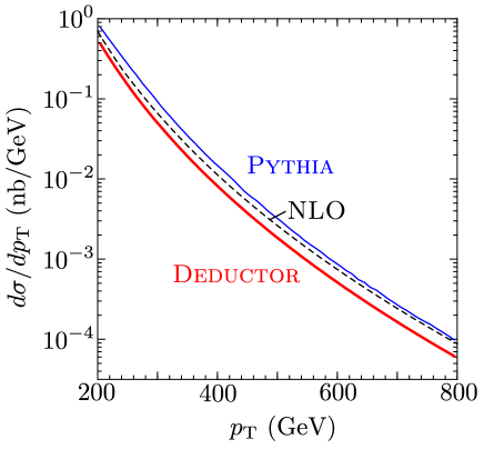
Figure 1: The one jet inclusive cross section $d\sigma/dp_{\mathrm{T}}$ for $|y|<2$ using the $k_{\mathrm{T}}$ algorithm with $R=0.4$ calculated with Deductor and Pythia. The dashed curve shows a next-to-leading order perturbative calculation.

3.3 Dijet angular decorrelation

The dijet angular decorrelation distribution is somewhat more subtle. We consider proton-proton collisions with $\sqrt{s}=8\ \mathrm{TeV}$. We use the $k_{\mathrm{T}}$ algorithm with $R=0.4$ to define jets and create a sample of events having at least two jets, each with $p_{\mathrm{T}}>200\ \mathrm{GeV}$ and $|y|<2$. Call the cross section for this $\sigma$. Let the azimuthal angle separation between the two jets with the highest $p_{\mathrm{T}}$ be $\phi$. Then we measure the distribution $\rho_{\phi}(\phi)=(1/\sigma)\,d\sigma/d\phi$ for this event sample. The normalization is $\int\!d\phi\ \rho_{\phi}(\phi)=1$. For an ideal two jet event, $\phi=\pi$. Emission of a soft gluon makes $\phi$ slightly less than $\pi$. Emission of a hard gluon that is not collinear with one of the two leading partons makes $\phi$ substantially less than $\pi$. For an ideal three jet event, $\phi$ can be as small as $2\pi/3$. Thus this angular distribution in the region $\phi>2\pi/3$ but $\pi-\phi$ not too small should be reliably predicted by fixed order perturbative QCD, while a parton shower should give a good account of it for $\pi-\phi\ll 1$. For these reasons, measurement of $\rho_{\phi}(\phi)$ provides a good experimental test of QCD D0Angles ; CMSAngles ; AtlasAngles . In figure 2, we compare the results of Deductor and Pythia for the dijet angular decorrelation. We see that the two results are very close to each other.

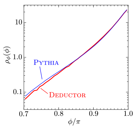
Figure 2: The angular decorrelation distribution, $\rho_{\phi}(\phi)$ for the two leading jets in an event with $P_{\mathrm{T}}>200\ \mathrm{GeV}$ and $|y|<2$, calculated with Deductor and Pythia.

3.4 Number of partons in a jet

In section 3.2 we looked at the one jet inclusive cross section. Now, we look inside these jets. We analyze a sample of jets with $P_{\mathrm{T}}>200\ \mathrm{GeV}$ and $|y|<2$. We examine the distribution $\rho_{n}(n)$ of the number $n$ of partons in a jet in this sample for events simulated by Pythia (with no hadronization or underlying event) and for events simulated by Deductor. The distribution is normalized to $\sum_{n}\rho_{n}(n)=1$. Evidently, the number of partons in a jet is not a physical observable, but it of interest here because it is sensitive to the parton showering algorithms. As explained in the introduction to this section, we adjust parameters of Pythia to make the results as comparable as we can between Pythia and Deductor. In figure 3, we compare the results of Deductor and Pythia for the distribution of the number of partons in a jet. We see that the distributions are similar but with a peak in the distribution for Deductor at $n=3$ and for Pythia at $n=4$.

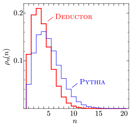
Figure 3: The distribution $\rho_{n}(n)$ of the number of partons in a Pythia jet with $P_{\mathrm{T}}>200\ \mathrm{GeV}$ and $|y|<2$ compared with the same distribution for a Deductor jet. The jets are constructed using the $k_{\mathrm{T}}$ algorithm with $R=0.4$.

3.5 $z$-distribution of partons in a jet

Again looking at the same sample of jets as in section 3.4, we can define a momentum fraction for each parton by $z=({\bm{p}}^{\rm parton}_{\mathrm{T}}\cdot{\bm{P}}_{\mathrm{T}}^{\rm jet})/({\bm{P}}_{\mathrm{T}}^{\rm jet})^{2}$. We can then measure the distribution of $z$ values, $f(z)=(1/N)\,dN/dz$. This distribution function obeys a momentum sum rule $\int_{0}^{1}\!dz\ zf(z)=1$. If we measured pions instead of partons, the function $f(z)$ would be an observable, the pion decay function of a jet. It would be a non-perturbative object, but with a perturbative evolution equation. In figure 4, we compare the results of Deductor to those of Pythia for $zf(z)$. There is a contribution proportional to $\delta(1-z)$ from jets that consist of one parton with $z=1$. This contribution is not seen in the plot.

We see that parton splitting above the cutoff defining the end of the shower is not quite as likely in Deductor as it is in Pythia, consistent with what we saw in section 3.4. Thus at the end of the shower Deductor has more hard partons and fewer soft partons than Pythia.

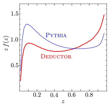
Figure 4: The $z$ distribution function of partons in a Pythia jet with $P_{\mathrm{T}}>200\ \mathrm{GeV}$ and $|y|<2$ compared with the same distribution for a Deductor jet. The jets are constructed using the $k_{\mathrm{T}}$ algorithm with $R=0.4$. We plot $zf(z)$.

3.6 Angular distribution of soft gluons between hard gluons

In this investigation, we examine quantum interference in the emission of a soft gluon. First, we generate a sample of events with large total transverse energy $E_{\mathrm{T}}>400\ \mathrm{GeV}$ (for partons with $|y|<3.6$). In each of these events, we use the $k_{\mathrm{T}}$ algorithm to identify jets made from partons with $|y|<3.6$. We use a very small jet radius parameter, $R=0.1$, so that we define the direction of the jets quite precisely. We demand that there be two jets, 1 and 2, that are fairly hard: $P_{T,1}>50\ \mathrm{GeV}$ and $P_{T,2}>50\ \mathrm{GeV}$. We further demand that the two jets be separated by an angle of about 0.5: defining $\theta^{2}_{12}=(y_{1}-y_{2})^{2}+(\phi_{1}-\phi_{2})^{2}$, we demand that $0.4<\theta_{12}<0.6$.

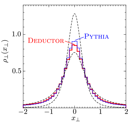
Figure 5: The distribution function, $\rho_{\perp}(x_{\perp})$, of a soft jet as a function of the angular variable $x_{\perp}$ as defined in the text. The distribution from Pythia is compared to that from Deductor. The function $\rho_{\perp}(x_{\perp};{\rm dipole})$ is displayed as the narrower dotted curve and the function $\rho_{\perp}(x_{\perp};{\rm independent})$ is displayed as the broader dashed curve.

Now, suppose that we identify the jets 1 and 2 with partons and that the system including these partons emits a soft gluon. Where does the soft gluon go? To find out, we find a third jet, 3, in the event, which we imagine is identified with the soft gluon. We demand that jet 3 have $P_{T,3}>4\ \mathrm{GeV}$. Then $P_{T,3}$ is typically just a little bigger than this minimum value, so jet 3 is fairly soft. We are interested in the angles, $y_{3}$ and $\phi_{3}$ of the soft jet. Define angular coordinates $x_{\parallel}$ and $x_{\perp}$ by

$$\begin{split}x_{\parallel}={}&\frac{(y_{3}-y_{1})(y_{2}-y_{1})+(\phi_{3}-\phi_{1})(\phi_{2}-\phi_{1})}{(y_{2}-y_{1})^{2}+(\phi_{2}-\phi_{1})^{2}}\;,\\ x_{\perp}={}&\frac{(\phi_{3}-\phi_{1})(y_{2}-y_{1})-(y_{3}-y_{1})(\phi_{2}-\phi_{1})}{(y_{2}-y_{1})^{2}+(\phi_{2}-\phi_{1})^{2}}\;.\end{split}$$ (3)

Thus jet 3 is in the same direction as jet 1 when $x_{\parallel}=0$ and $x_{\perp}=0$, while it is in the same direction as jet 2 when $x_{\parallel}=1$ and $x_{\perp}=0$. The point just between the directions of the two hard jets is $x_{\parallel}=1/2$ and $x_{\perp}=0$. The soft jet has the same absolute angular separation from each of the two hard jets along the line $x_{\parallel}=1/2$ with varying $x_{\perp}$. We demand that $x_{\parallel}$ be near $x_{\parallel}=1/2$, in a range $1/3<x_{\parallel}<2/3$. We are interested in the distribution of $x_{\perp}$ when $x_{\parallel}$ is in this range. Let $\rho_{\perp}(x_{\perp})\,dx_{\perp}$ be the probability that jet 3 has the specified value of $x_{\perp}$ when $x_{\parallel}$ is in the required range and all of the other cut conditions are satisfied. We examine the range $-2<x_{\perp}<2$. Thus we normalize $\rho_{\perp}(x_{\perp})$ to

$$\int_{-2}^{2}\!dx_{\perp}\,\rho_{\perp}(x_{\perp})=1\;.$$ (4)

What do we expect for $\rho_{\perp}(x_{\perp})$?

We may expect that $\rho_{\perp}(x_{\perp})$ has a contribution from background jets that are not correlated with partons 1 and 2. Part of this contribution will come from initial state radiation, for instance. Thus we expect a contribution proportional to

$$\rho_{\perp}(x_{\perp};{\rm background})=\frac{1}{{\cal N}({\rm background})}\;,$$ (5)

where ${\cal N}({\rm background})$ is a constant (which will depend on the various parameters that go into the definitions). The factor ${\cal N}({\rm background})$ is a normalization factor. We define it and two other normalization factors below.

We also expect a contribution corresponding to independent emissions of soft gluons from either parton 1 or parton 2. This contribution will be proportional to

$$\rho_{\perp}(x_{\perp};{\rm independent})=\frac{1}{{\cal N}({\rm independent})}\,\frac{1}{(0.5)^{2}+x_{\perp}^{2}}\;.$$ (6)

Here $(0.5)^{2}+x_{\perp}^{2}$ is $x_{\parallel}^{2}+x_{\perp}^{2}$ or $(1-x_{\parallel})^{2}+x_{\perp}^{2}$, where $x_{\parallel}=0.5$ is the position of the center of the $x_{\parallel}$-bin.

Finally, we expect a contribution corresponding to emissions of soft gluons from the dipole consisting partons 1 and 2 (or a dipole consisting of partons moving parallel to these partons). This contribution will be proportional to

$$\rho_{\perp}(x_{\perp};{\rm dipole})=\frac{1}{{\cal N}({\rm dipole})}\,\left[\frac{1}{(0.5)^{2}+x_{\perp}^{2}}\right]^{2}\;.$$ (7)

In a partitioned dipole shower, this contribution is generated in two parts, attributed to emission from parton 1 and from parton 2. Here we put the two parts together. Note that in this contribution, emission for $|x_{\perp}|>0.5$ is suppressed because of destructive quantum interference. That is, there is approximate angular ordering. However, there is no suppression for $|x_{\perp}|<0.5$ because there is constructive quantum interference.

We have left normalization factors ${\cal N}$ undefined so far. We define these factors so that the distributions $\rho_{\perp}(x_{\perp};{\rm background})$, $\rho_{\perp}(x_{\perp};{\rm independent})$, and $\rho_{\perp}(x_{\perp};{\rm dipole})$ are normalized on $-2<x_{\perp}<2$, as in eq. (4). Thus

$$\begin{split}{\cal N}({\rm background})={}&4\;,\\ {\cal N}({\rm independent})={}&4\arctan(4)\;,\\ {\cal N}({\rm dipole})={}&32/17+8\arctan(4)\;.\end{split}$$ (8)

In figure 5, we compare the results of Deductor to those of Pythia for $\rho_{\perp}(x_{\perp})$. We see that the shapes are very similar, but that the Pythia curve is slightly narrower than the Deductor curve. We also show the functions $\rho_{\perp}(x_{\perp};{\rm dipole})$ and $\rho_{\perp}(x_{\perp};{\rm independent})$. To understand the results quantitatively we fit $\rho_{\perp}(x_{\perp})$ for Pythia and Deductor to the form

$$\begin{split}\rho_{\perp}(x_{\perp})={}&C({\rm background})\,\rho_{\perp}(x_{\perp};{\rm background})\\ &+C({\rm independent})\,\rho_{\perp}(x_{\perp};{\rm independent})\\ &+C({\rm dipole})\,\rho_{\perp}(x_{\perp};{\rm dipole})\;.\end{split}$$ (9)

In both cases, we find that $C({\rm background})$ is small enough that we can ignore it. Then for Pythia we find that $C({\rm independent})\approx 0.68$, $C({\rm dipole})\approx 0.32$. For Deductor, $C({\rm independent})\approx 0.78$, $C({\rm dipole})\approx 0.22$. We judge that the difference between Pythia and Deductor is not very important but that it is important that one can see the quantum interference effect that is built into both these programs.

3.7 Transverse momentum distribution of vector bosons

We examine next the production $e^{+}e^{-}$ pairs produced from a Z-boson or photon in a proton-proton collision with $\sqrt{s}=8\ \mathrm{TeV}$. We are interested in the transverse momentum, $p_{\mathrm{T}}$, of the $e^{+}e^{-}$ pair. We demand that the mass of the $e^{+}e^{-}$ pair be large, $M(e^{+}e^{-})>400\ \mathrm{GeV}$, and that its rapidity be in the central region, $|y(e^{+}e^{-})|<2$, and we look at the region of small and moderate transverse momentum, $0<p_{\mathrm{T}}<100\ \mathrm{GeV}$. We measure the distribution $\rho_{\mathrm{Z}}(p_{\mathrm{T}})=(1/\sigma)\,d\sigma/dp_{\mathrm{T}}$ for this event sample. The normalization is $\int_{0}^{100\ \mathrm{GeV}}\!dp_{\mathrm{T}}\ \rho_{\mathrm{Z}}(p_{\mathrm{T}})=1$.

We compare the result from Deductor to that from Pythia in figure 6. We see that the curve from Deductor is somewhat narrower than that from Pythia. There are non-perturbative effects that are missing in Deductor and have been turned off in Pythia. There are also effects from the choice of how the perturbative shower is ended. These effects can have the effect of changing the width of the distributions and are especially important for $p_{\mathrm{T}}<10\ \mathrm{GeV}$. Thus it seems plausible that non-perturbative and shower-end effects account for the difference between the Deductor and Pythia curves.

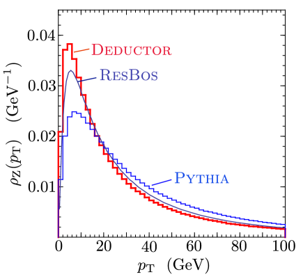
Figure 6: The transverse momentum distribution $\rho_{\mathrm{Z}}(p_{\mathrm{T}})$ of $e^{+}e^{-}$ pairs produced in the Drell-Yan process. We compare the distribution from Deductor to that Pythia and also to the distribution from ResBos, which sums logs of $p_{\mathrm{T}}/M(e^{+}e^{-})$. See the text for details. In the left hand portion of the figure, the top curve is Deductor, the middle curve is Resbos, and the lower curve is Pythia

There is a theoretical result CSSpT for the structure of $\rho_{\mathrm{Z}}(p_{\mathrm{T}})$ after summing logs of $p_{\mathrm{T}}/M$. This result, including a fit to nonperturbative effects that smear the distribution slightly, is available in the computer program ResBos, by C. Balazs, P. Nadolsky, and C.P. Yuan ResBos1 ; ResBos4 ; ResBos20 . We also show a result from ResBos in figure 6. Our ResBos results are for a virtual $Z$-boson rather than a linear combination of a virtual $Z$-boson and a virtual photon as simulated in Deductor and Pythia. In the region that we study, this difference should affect the normalization of the cross section but its effect on the shape should be small.

A dipole shower, as in Deductor, approximately sums the logs of $P_{\mathrm{T}}/M$ NSDrellYan . Thus we expect Deductor and ResBos results for $\rho_{\mathrm{Z}}(p_{\mathrm{T}})$ to agree approximately. It seems plausible that adjusting how the shower ends and including nonperturbative effects can broaden the Deductor result slightly to bring it into better agreement with ResBos.

3.8 Transverse momentum distribution of associated b-quarks

Initial state b-quarks and c-quarks are have non-zero masses in Deductor but are treated as massless in Pythia. Does this make a difference? To investigate this question, we simulate the production of an $e^{+}e^{-}$ pair in the Drell-Yan process, as in the previous subsection. However we demand that the $\mathrm{Z}$ or $\gamma$ be produced by a collision of a $\mathrm{b}$-quark and a $\bar{\mathrm{b}}$-quark, where the b-quark comes from the proton with positive $p^{3}$. Of course, a $\mathrm{Z}$ or $\gamma$ can be created by annihilation of any flavor of quark with its corresponding antiquark, but we examine only the b-quark process. Consider the b-quark that annihilates to make the $\mathrm{Z}$ or $\gamma$. In the backwards evolution of the initial state, this b-quark eventually becomes a gluon, with the emission of a $\bar{\mathrm{b}}$ quark. Where does the $\bar{\mathrm{b}}$ quark go?

We define $\rho_{Y}(\Delta y)\,d\Delta y$ to be the probability for the $\bar{\mathrm{b}}$ quark to have rapidity $\Delta y$ relative to the rapidity of the $e^{+}e^{-}$ pair, $\Delta y=y(\bar{\mathrm{b}})-y(e^{+}e^{-})$, normalized to $\int_{-5}^{5}\!d\Delta y\,\rho_{Y}(\Delta y)=1$. In the left hand plot of figure 7, we compare the result for $\rho_{Y}(\Delta y)$ from Deductor to that from Pythia. We see that there is hardly any difference.

We define $\rho_{\mathrm{T}}(p_{\mathrm{T}})\,dp_{\mathrm{T}}$ to be the probability for the $\bar{\mathrm{b}}$ quark to have transverse momentum $p_{\mathrm{T}}$, normalized to $\int_{0}^{30\ \mathrm{GeV}}\!dp_{\mathrm{T}}\,\rho_{\mathrm{T}}(p_{\mathrm{T}})=1$. In the right hand plot, we compare the result for $\rho_{\mathrm{T}}(p_{\mathrm{T}})$ from Deductor to that from Pythia. There is hardly any difference except near $p_{T}$ equal the the b-quark mass $m(\mathrm{b})$, which is 4.75 GeV in Deductor. Near $p_{\mathrm{T}}=m(\mathrm{b})$, the Deductor curve has a peak. This seems sensible according to the kinematics of the process $\mathrm{g}\to\mathrm{b}+\bar{\mathrm{b}}$. Near $p_{\mathrm{T}}=m(\mathrm{b})$, the Pythia histogram has a dip. Presumably this is because initial state quarks are treated as massless in Pythia. These results are before transverse momentum smearing of the incoming partons and before hadronization. We expect that after these effects, the Pythia dip will be washed out.

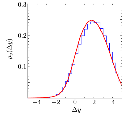
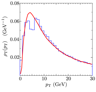
Figure 7: The distribution of $\bar{\mathrm{b}}$-quarks in events with the hard process $\mathrm{b}+\bar{\mathrm{b}}\to\mathrm{Z}/\gamma+X\to e^{+}+e^{-}+X$ with $M(e^{+}e^{-})>400\ \mathrm{GeV}$ and $|y(e^{+}e^{-})|<2$. The left hand plot compares the distribution in rapidity $\Delta y=y(\bar{\mathrm{b}})-y(e^{+}e^{-})$ from Deductor (the curve) and Pythia (the histogram). The right hand plot compares the distributions in transverse momentum $p_{\mathrm{T}}(\bar{\mathrm{b}})$. Again, the curve is from Deductor and the histogram is from Pythia.

4 Conclusions

We have presented some first results from a new parton shower Monte Carlo event generator, Deductor, which generates events from a hard scattering process and both initial state and final state parton showers. Hadronization and an underlying event are not included in this initial version. Our main purpose in creating this event generator was to investigate the effects of parton color and spin. However, in this paper, we confine our investigation to the leading color, spin averaged approximation. The code implements also the LC+ approximation NScolor , which we will compare to the leading color approximation in a future work. There is a straightforward algorithm NSspin for improving the treatment of spin, but this algorithm is not yet implemented.

There are some new features in Deductor compared to other parton shower event generators. Shower splittings are generated according to a virtuality based ordering variable $\Lambda^{2}$ defined in eq. (1) instead of transverse momentum $k_{\mathrm{T}}$. This is discussed in a companion paper NSShowerTime . Deductor does not follow the standard practice of setting the masses of initial state b and c quarks to zero. This requires new evolution kernels for the parton distribution functions. This is discussed in a companion paper NSpartons .

We have compared results from Deductor to results from Pythia for a number of distributions that illustrate the workings of a parton shower. We find that there are some differences but that they are not large. As seen in figure 5, both programs exhibit the effect of quantum interference between soft gluon emissions from a color dipole. With the shower-end settings that we used, Deductor has somewhat fewer splittings than Pythia. Jet cross sections are comparable, as are the transverse momentum distributions of Drell-Yan lepton pairs. By looking in the right place, one can observe differences that result from the different treatment of parton mass for initial state b-quarks.

The comparisons that we have generated suggest that Deductor is working sensibly. It remains to investigate the effects of including better approximations for color and spin.

- (1) G. Marchesini, B. R. Webber, G. Abbiendi, I. G. Knowles, M. H. Seymour and L. Stanco, HERWIG: A Monte Carlo event generator for simulating hadron emission reactions with interfering gluons, Comput. Phys. Commun. 67 (1992) 465 [INSPIRE]; M. Bahr, S. Gieseke, M. A. Gigg, D. Grellscheid, K. Hamilton, O. Latunde-Dada, S. Platzer and P. Richardson et al., Herwig++ Physics and Manual, Eur. Phys. J. C 58 (2008) 639 [arXiv:0803.0883 [hep-ph]] [INSPIRE].
- (2) T. Sjöstrand, High-energy physics event generation with PYTHIA 5.7 and JETSET 7.4, Comput. Phys. Commun. 82 (1994) 74 [INSPIRE]; T. Sjostrand, S. Mrenna and P. Z. Skands, A Brief Introduction to PYTHIA 8.1, Comput. Phys. Commun. 178 (2008) 852 [arXiv:0710.3820 [hep-ph]] [INSPIRE].
- (3) T. Gleisberg, S. Hoeche, F. Krauss, M. Schonherr, S. Schumann, F. Siegert and J. Winter, Event generation with SHERPA 1.1, JHEP 0902 (2009) 007 [arXiv:0811.4622 [hep-ph]] [INSPIRE].
- (4) T. Sjöstrand, A Model for initial state parton showers, Phys. Lett. B 157 (1985) 321 [INSPIRE].
- (5) T. D. Gottschalk, Backwards evolved initial state parton showers, Nucl. Phys. B 277 (1986) 700 [INSPIRE].
- (6) G. Marchesini and B. R. Webber, Simulation Of QCD jets including soft gluon interference, Nucl. Phys. B 238 (1984) 1 [INSPIRE]; R. K. Ellis, G. Marchesini and B. R. Webber, Soft radiation in parton parton scattering, Nucl. Phys. B 286 (1987) 643 [Erratum-ibid. B 294 (1987) 1180] [INSPIRE].
- (7) Z. Nagy and D. E. Soper, Parton showers with quantum interference, JHEP 0709 (2007) 114 [arXiv:0706.0017 [hep-ph]] [INSPIRE].
- (8) Z. Nagy and D. E. Soper, Parton showers with quantum interference: leading color, spin averaged, JHEP 0803 (2008) 030 [arXiv:0801.1917 [hep-ph]] [INSPIRE].
- (9) The code is available at http://www.desy.de/znagy/deductor/ and http://pages.uoregon.edu/soper/deductor/.
- (10) Z. Nagy and D. E. Soper, Parton shower evolution with subleading color, JHEP 1206 (2012) 044 [arXiv:1202.4496 [hep-ph]] [INSPIRE].
- (11) Z. Nagy and D. E. Soper, Parton showers with quantum interference: Leading color, with spin, JHEP 0807 (2008) 025 [arXiv:0805.0216 [hep-ph]] [INSPIRE].
- (12) T. Sjostrand and P. Z. Skands, Transverse-momentum-ordered showers and interleaved multiple interactions, Eur. Phys. J. C 39 (2005) 129 [hep-ph/0408302] [INSPIRE].
- (13) Z. Nagy and D. E. Soper, Ordering variable for parton showers, (to be submitted).
- (14) Z. Nagy and D. E. Soper, Parton distribution functions in the context of parton showers, (to be submitted).
- (15) Z. Nagy and D. E. Soper, On the transverse momentum in Z-boson production in a virtuality ordered parton shower, JHEP 1003 (2010) 097 [arXiv:0912.4534 [hep-ph]] [INSPIRE].
- (16) R. Doria, J. Frenkel and J. C. Taylor, Counter Example to Nonabelian Bloch-Nordsieck Theorem, Nucl. Phys. B 168 (1980) 93 [INSPIRE].
- (17) J. C. Collins, D. E. Soper and G. F. Sterman, Factorization for Short Distance Hadron - Hadron Scattering, Nucl. Phys. B 261 (1985) 104 [INSPIRE]; J. C. Collins, D. E. Soper and G. F. Sterman, Soft Gluons and Factorization, Nucl. Phys. B 308 (1988) 833 [INSPIRE].
- (18) V. N. Gribov and L. N. Lipatov, Deep inelastic scattering in perturbation theory, Sov. J. Nucl. Phys. 15, 438 (1972) [Yad. Fiz. 15, 781 (1972)] [INSPIRE]; G. Altarelli and G. Parisi, Asymptotic freedom in parton language, Nucl. Phys. B 126, 298 (1977) [INSPIRE]; Y. L. Dokshitzer, Calculation of the structure functions for deep inelastic scattering and annihilation by perturbation theory in quantum chromodynamics, (in Russian), Sov. Phys. JETP 46, 641 (1977) [Zh. Eksp. Teor. Fiz. 73, 1216 (1977)] [INSPIRE].
- (19) J. C. Collins and D. E. Soper, Parton Distribution and Decay Functions, Nucl. Phys. B 194 (1982) 445 [INSPIRE].
- (20) F. D. Aaron et al. [H1 and ZEUS Collaboration], Combined Measurement and QCD Analysis of the Inclusive e+- p Scattering Cross Sections at HERA, JHEP 1001 (2010) 109 [arXiv:0911.0884 [hep-ex]] [INSPIRE].
- (21) F. D. Aaron et al. [H1 Collaboration], A Precision Measurement of the Inclusive ep Scattering Cross Section at HERA, Eur. Phys. J. C 64 (2009) 561 [arXiv:0904.3513 [hep-ex]] [INSPIRE].
- (22) S. Catani, B. R. Webber and G. Marchesini, QCD coherent branching and semiinclusive processes at large , Nucl. Phys. B 349 (1991) 635 [INSPIRE].
- (23) A. D. Martin, W. J. Stirling, R. S. Thorne and G. Watt, Parton distributions for the LHC, Eur. Phys. J. C 63 (2009) 189 [arXiv:0901.0002 [hep-ph]] [INSPIRE].
- (24) S. Catani, Y. L. Dokshitzer, M. H. Seymour, and B. R. Webber, Longitudinally invariant clustering algorithms for hadron hadron collisions, Nucl. Phys. B 406 (1993) 187 [INSPIRE].
- (25) S. D. Ellis and D. E. Soper, Successive combination jet algorithm for hadron collisions, Phys. Rev. D 48 (1993) 3160 [hep-ph/9305266] [INSPIRE].
- (26) M. Cacciari, G. P. Salam and G. Soyez, FastJet User Manual, Eur. Phys. J. C 72 (2012) 1896 [arXiv:1111.6097 [hep-ph]] [INSPIRE].
- (27) S. D. Ellis, Z. Kunszt and D. E. Soper, The One Jet Inclusive Cross-section at Order Quarks and Gluons, Phys. Rev. Lett. 64 (1990) 2121 [INSPIRE].
- (28) H. -L. Lai, M. Guzzi, J. Huston, Z. Li, P. M. Nadolsky, J. Pumplin and C. -P. Yuan, New parton distributions for collider physics, Phys. Rev. D 82 (2010) 074024 [arXiv:1007.2241 [hep-ph]] [INSPIRE].
- (29) V. M. Abazov et al. [D0 Collaboration], Measurement of dijet azimuthal decorrelations at central rapidities in collisions at TeV, Phys. Rev. Lett. 94 (2005) 221801 [hep-ex/0409040] [INSPIRE].
- (30) V. Khachatryan et al. [CMS Collaboration], Dijet Azimuthal Decorrelations in Collisions at TeV, Phys. Rev. Lett. 106 (2011) 122003 [arXiv:1101.5029 [hep-ex]] [INSPIRE].
- (31) G. Aad et al. [ATLAS Collaboration], Measurement of Dijet Azimuthal Decorrelations in Collisions at TeV, Phys. Rev. Lett. 106 (2011) 172002 [arXiv:1102.2696 [hep-ex]] [INSPIRE].
- (32) J. C. Collins, D. E. Soper and G. F. Sterman, Transverse Momentum Distribution in Drell-Yan Pair and W and Z Boson Production, Nucl. Phys. B 250 (1985) 199. [INSPIRE].
- (33) G. A. Ladinsky and C. P. Yuan, The Nonperturbative regime in QCD resummation for gauge boson production at hadron colliders, Phys. Rev. D 50 (1994) 4239 [hep-ph/9311341] [INSPIRE].
- (34) C. Balazs and C. P. Yuan, Soft gluon effects on lepton pairs at hadron colliders, Phys. Rev. D 56 (1997) 5558 [hep-ph/9704258] [INSPIRE].
- (35) F. Landry, R. Brock, P. M. Nadolsky and C. P. Yuan, Tevatron Run-1 boson data and Collins-Soper-Sterman resummation formalism, Phys. Rev. D 67 (2003) 073016 [hep-ph/0212159] [INSPIRE].