Control of Multiple Remote Servers
for Quality-Fair Delivery of Multimedia Contents

Abstract

This paper proposes a control scheme for the quality-fair delivery of several encoded video streams to mobile users sharing a common wireless resource. Video quality fairness, as well as similar delivery delays are targeted among streams. The proposed controller is implemented within some aggregator located near the bottleneck of the network. The transmission rate among streams is adapted based on the quality of the already encoded and buffered packets in the aggregator. Encoding rate targets are evaluated by the aggregator and fed back to each remote video server (fully centralized solution), or directly evaluated by each server in a distributed way (partially distributed solution). Each encoding rate target is adjusted for each stream independently based on the corresponding buffer level or buffering delay in the aggregator. Communication delays between the servers and the aggregator are taken into account.

The transmission and encoding rate control problems are studied with a control-theoretic perspective. The system is described with a multi-input multi-output model. Proportional Integral (PI) controllers are used to adjust the video quality and control the aggregator buffer levels. The system equilibrium and stability properties are studied. This provides guidelines for choosing the parameters of the PI controllers.

Experimental results show the convergence of the proposed control system and demonstrate the improvement in video quality fairness compared to a classical transmission rate fair streaming solution and to a utility max-min fair approach.

I Introduction

With the development of wireless networks and widespread of smartphones, delivery of compressed videos (video-on-demand or mobile TV broadcast services) to mobile users is increasing rapidly. This trend is likely to continue in the coming years [1]. To satisfy the related increasing demand for resources, operators have to expand their network capacity with as limited as possible infrastructure investments. In parallel, they have to optimize the way multimedia contents are delivered to users while satisfying application-layer quality-of-service (QoS) constraints, which are more challenging to address than traditional network-layer QoS constraints.

Delivered videos have a large variety of quality-rate characteristics, whatever the considered quality metric, e.g., Peak Signal-to-Noise Ratio (PSNR), Structural SIMilarity (SSIM) [2], etc. These characteristics are time-varying and depend on the content of the videos. Provisioning some constant transmission rate to mobile users for video delivery is in general inappropriate. If videos are encoded at a constant bitrate, the quality may fluctuate with the variations of the characteristics of the content. If they are encoded at a variable bitrate, targeting a constant quality, buffering delays may fluctuate significantly.

This paper proposes a controller for the quality-fair delivery of several encoded video streams to mobile users sharing a common wireless resource. Video-on-demand or multicast/broadcast transmission are typical applications for this scenario. Video encoding rate adaptation and wireless resource allocation are performed jointly within some Media Aware Network Element (MANE) using feedback control loops. The aim is to provide users with encoded videos of similar quality and with controlled delivery delay, without exchanging information between remotely located video servers.

I-A Related work

When controlling the parallel delivery of several video streams, their rate-distortion (R-D) trade-off may be adjusted by selectively discarding frames as in [3, 4] or via an adaptation of their encoding parameters as in [5, 6]. With scalable video encoders, such as H.264/SVC, the R-D trade-off may be adjusted via packet filtering [7, 8]. In this case, the control parameter is the number of transmitted enhancement layers for each frame.

If several video streams are transmitted to different users in a dedicated broadcast channel with limited capacity, a blind source rate allocation could lead to unacceptable quality for high-complexity video contents compared to low-complexity ones. Therefore, providing fairness is an important issue that must be addressed.

Video quality fairness among encoded streams may be obtained by sharing quality information, or R-D characteristics via a central controller providing to each server quality or rate targets, as in [9, 10]. This technique enables the encoders to adjust their bit rate or to drop frames or quality layers depending on the complexity of the videos and on the available transmission rate.

Control-theoretic approaches have been considered to address the problem of rate control in the context of video streaming, see, e.g., [11, 12, 13, 14, 15]. In [11], a real-time rate control based on a Proportional Integral Derivative (PID) controller is proposed for a single video stream. The main idea is to determine the encoding rate per frame based on the buffer level to maximize video quality and minimize quality variations over frames. In [12], a flow control mechanism with active queue management and a proportional controller is considered. A flow control is used to reduce the buffer size and avoid buffer overflow and underflow. The flow control mechanism is shown to be stable for small buffer sizes and non-negligible round-trip times. In [13], a rate allocation algorithm, performed at the Group of Picture (GoP) level, is performed at the sender to maximize the visual quality according to the overall loss and the receiver buffer occupancy. This target is achieved using a Proportional Integral (PI) controller in charge of determining the transmission rate to drain the buffers. Later, [16] introduces a rate controller that uses different bit allocation strategies for Intra and Inter frames. A PID controller is adopted to minimize the deviations between the target and the current buffer level. Buffer management is performed at the bit level and delivery delay is not considered. Moreover, [11, 12, 13, 16] address single flow transmission.

For multi-video streaming, in [17], a distributed utility max-min flow control in the presence of round-trip delays is proposed. The distributed link algorithm performs utility max-min bandwidth sharing while controlling the link buffer occupancy around a target value at the cost of link under utilization using a PID controller. Stability analysis in case of a single bottleneck and homogeneous delay is conducted. In [9], a content-aware distortion-fair video delivery scheme is proposed to deliver video streams based on the characteristics of video frames. It provides a max-min distortion fair resource sharing among video streams. The system uses temporal prediction structure of the video sequences with a frame drop strategy based on the frame importance to guide resource allocation. The proposed scheme is for video on-demand services, where the rate and the importance of each frame are assumed calculated in advance. A proportional controller is considered in [14] to stabilize the received video quality as well as the bottleneck link queue for both homogeneous and heterogeneous video contents. A PI controller is considered in [15]. Robustness and stability properties are studied. In [14] and [15], the rate control is performed in a centralized way, exploiting the rate and distortion characteristics of the considered video flows to determine the encoding rate for the next frame of each flow. In [18], a cross-layer optimization framework for scalable video delivery over OFDMA wireless systems is proposed, aiming at maximizing the sum of the achievable rates while minimizing the distortion difference among multiple videos. The optimization problem is described by a Lagrangian constrained sum-rate maximization to achieve distortion fairness among users. However the communication delay between the control block and the controlled servers is not addressed.

Remotely implemented control laws are also considered in [19] leading to the problem of stabilizing an open-loop system with time-varying delay. The problem of remote stabilization via communication networks is considered with an explicit use of the average network dynamics and an estimation of the average delay in the control law. The control law does not address video transmission issues, so no quality constraint on the transmitted data is considered.

The commercial products described in [20, 21] propose statistical multiplexing systems enabling encoders to adapt their outputs to the available channel rate. Connecting encoders and multiplexers via a switched IP network allows collocated and distributed encoders to be part of the multiplexing system. Nevertheless, in these solutions, quality fairness constraints between programs appear not to be considered among the video quality constraints.

I-B Main contributions

In this paper, we propose a control system to perform jointly (i) encoding rate control of spatially spread video servers without information exchange between them and (ii) transmission rate control of the encoded streams through some bottleneck link. A MANE, located near the bottleneck link derives the average video quality of the data stored in dedicated buffers fed by the remote servers. This average video quality is compared by each individual transmission rate controller to the quality of its video flow to adjust the draining rate of the corresponding buffer (first control input). For that purpose, programs with low quality are drained faster than programs with high quality. Dedicated encoding rate controllers observe the buffer levels to adjust the video encoding rates (second control input). The encoding rate control targets a similar buffer level for all programs. The buffer level in bits or the buffering delay can be adjusted via an adaptation of the video encoding rates, e.g., by scalability layer filtering when a scalable video coder is involved.

In a fully centralized version of the controller, the MANE is in charge of sending the encoding rate target to each video server. In a partly distributed version, only the individual buffer level discrepancies are transmitted to the servers, which are then in charge of computing their own encoding rate target. Communication delays between the MANE and the servers are considered in both directions. A discrete-time state-space representation of the system is introduced. The buffer level (in bits) or the buffering delay has to be controlled and quality fairness between video streams has to be obtained. For that purpose, feedback loops involving PI controllers are considered. The quality fairness constraint among streams leads to a coupling of the state equations related to the control of the delivery of each stream. The system equilibrium and stability properties are studied. This provides guidelines for choosing the parameters of the PI controllers. This paper extends preliminary results obtained in [22], where control of the buffer level in bits is not addressed and the communication delay between the MANE and the servers is not explicitly considered.

Section II introduces the considered system and the constraints that have to be satisfied. The proposed solution is described in Section III. The required hypotheses are listed and a discrete-time state-space representation of the system is provided, emphasizing the coupling between equations induced by the fairness constraint among video streams. The equilibrium and stability analyses are performed in Section IV. Finally, a typical application context is described in Section V and experimental results are detailed. Robustness of the proposed control system to variations of the channel rate and of the number of video streams is shown.

II System description

Consider a communication system in which $N$ encoded video streams provided by $N$ remote servers arrive to some network bottleneck where they have to share a communication channel providing a total transmission rate $R^{\text{c}}$, see Figure 1. The servers deliver encoded Video Units (VUs) representing a single picture or a Group of Pictures (GoP). All VUs are assumed to be of the same duration $T$ and the frame rate $F$ is assumed constant over time and identical for all streams. Time is slotted and the $j$-th time index represents the time interval $\left[jT,\left(j+1\right)T\right)$.

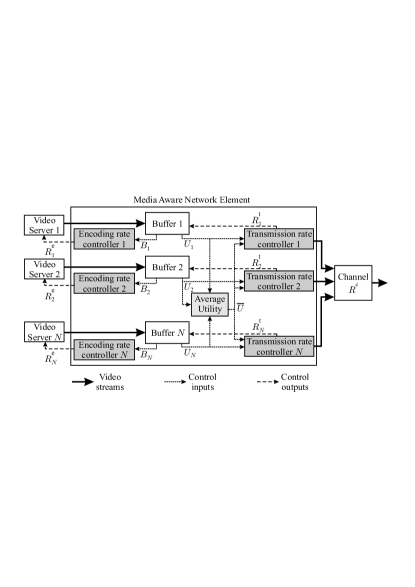
Figure 1: Structure of the proposed quality-fair video delivery system (fully centralized version).

In the proposed system, a Media Aware Network Element (MANE) is located close to the bottleneck of the network, see Figure 1. The MANE aims at providing the receivers with video streams of similar (objective or subjective) quality and with similar delivery delays. For that purpose, two feedback loops are considered to control (i) the encoding rate and (ii) the transmission rate of each video stream, see Figure 2.

Encoded and packetized VUs are temporarily stored in dedicated buffers in the MANE. We assume that a utility $U_{i}\left(j\right)$ measures the quality of each VU $j$ for each stream $i$ (in terms of PSNR, SSIM, or any other video quality metric [23]). The MANE has access to $U_{i}\left(j\right)$, stored, e.g., in the packet headers. The transmission rate controllers are in charge of choosing the draining rates from each buffer so that all utilities within the $N$ buffers are as close as possible. The encoding rate controllers are in charge of choosing the video encoding rates so that the buffer levels in the MANE are adjusted around some reference level $B_{0}$ in bits or reference delay $\tau_{0}$ in seconds. This control is performed at each discrete time index.

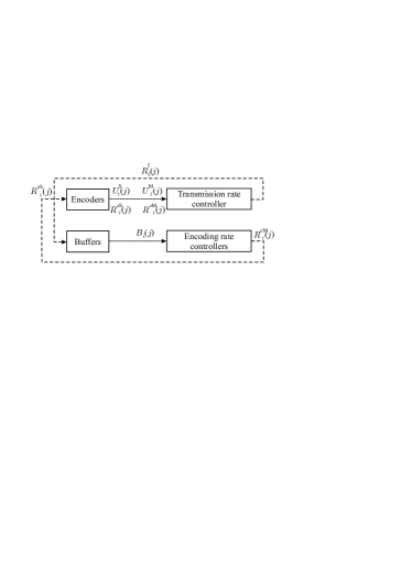
Figure 2: Feedback control loops in the proposed quality-fair video delivery system.

The MANE evaluates the average utility and each transmission rate controller allocates more rate to streams with a utility below average. The buffers of these streams are drained faster than those with utility above average. This control, done within the MANE, is thus centralized. The discrepancy of each buffer level in bits (respectively delay in seconds) with respect to the reference level $B_{0}$ (respectively delay $\tau_{0}$) is processed individually by an encoding rate controller. The encoding rate for the next VU of each video stream is then evaluated to regulate the buffer level around the reference level. The encoding rate may be evaluated at the MANE, in which case, the control is fully centralized and the video encoders/servers receive only the evaluated target bit rate. Alternatively, the encoding rates may be evaluated in a decentralized way at each video encoder/server. For the latter case, the MANE only feeds back to each server the buffer level (respectively delay) discrepancy. This solution requires all video encoders/servers to host individually an encoding rate controller, which is mainly possible for managed video servers. In this paper, the encoding rate target is evaluated within the MANE, but the encoding parameters are evaluated in a distributed way by each server [24].

The interaction of both control loops (transmission rate control and encoding rate control) allows getting a quality-fair video delivery. Videos with a quality below average have a buffer in the MANE that is drained faster, and thus is likely to be below $B_{0}$ or $\tau_{0}$. The encoding rate of such streams is then increased, to improve their quality.

Feedback delays between the MANE and the video servers are considered. They correspond to the delays introduced when the servers deliver encoded packets to the MANE and when the MANE feeds back signalization to carry encoding rate targets to the servers. To account for the delayed utility available at the MANE and the delayed encoding rate targets sent by the MANE to the servers, two state variables representing the delayed encoding rates and the delayed utilities are introduced

$$R_{i}^{\text{eS}}\left(j\right)=R_{i}^{\text{eM}}\left(j-\delta_{1}\right),$$ (1)

and

$$U_{i}^{\text{M}}\left(j\right)=U_{i}^{\text{S}}\left(j-\delta_{2}\right),$$ (2)

where $R_{i}^{\text{eM}}(j)$ is the encoding rate evaluated at the MANE for the $j$-th VU of program $i$. This encoding rate target reaches the server with some delay $\delta_{1}$, where it is denoted by $R_{i}^{\text{eS}}(j)$. On the other hand, the server sends the utility of the $j$-th VU of program $i$, denoted by $U_{i}^{\text{S}}(j)$. It arrives at the MANE with some delay $\delta_{2}$ and is denoted $U_{i}^{\text{M}}(j)$, see Figure 2. The M superscript refers to the information available at the MANE and the S superscript refers to the information available at the server for both rate and utility. In what follows, the stability of both control loops is studied.

III State-space representation

A state-space representation of the system presented in Section II is introduced to study its stability. Several additional assumptions are needed to get a tractable representation.

III-A Assumptions

III-A1 Feedback delay

In what follows, a VU represents a GoP. All encoded VUs processed by the video servers during the $\left(j-1\right)$-th time slot $\left[(j-1)T,jT\right)$ are assumed to have reached the MANE during the $j$-th time slot $\left[jT,\left(j+1\right)T\right)$. The encoding rate targets sent by the MANE to the servers $R_{i}^{\text{e}}(j)$ at the beginning of the $j$-th time slot are assumed to have reached all video servers at the beginning of the $\left(j+1\right)$-th time slot. This rate is used to encode the $\left(j+1\right)$-th VU which will be placed in the buffer in the MANE during the $\left(j+2\right)$-th time slot, etc., see Figure 3 when $\delta_{1}=\delta_{2}=1$.

The transmission delays between the MANE and the servers may vary. The previous assumptions allow to cope with forward and backward delays upper bounded by $T$. This is reasonable, since the network transmission and buffering delays are of the order of tens of milliseconds, provided that it is not too congested. This is less than the duration of VUs when they represent GoPs (typically $0.25$ s to $1$ s). Following the bounded-delay assumption, during the $j$-th time slot, the MANE has only access to the utilities $U_{i}^{\text{S}}(j-2)$, $i=1,\dots,N$ of the $\left(j-2\right)$-th encoded VUs.

In the rest of the paper the superscripts S and M are omitted. Then $U_{i}\left(j\right)$ is the utility of the $j$-th VU of the $i$-th stream encoded during time slot $j$, transmitted to the MANE during time slot $j+1$, and fully buffered in the MANE at the beginning of time slot $j+2$. $R^{\text{e}}(j)$ is the encoding rate target evaluated by the MANE during the $j$-th time slot. $R^{\text{e}}(j)$ reaches the server at the beginning of time slot $j+1$, see Figure 3.

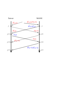
Figure 3: Communication delays between a video server and the MANE.

III-A2 Source model

The following parametric rate-utility model is used to describe the evolution of the utility $U_{i}(j)$ as a function of the rate $R_{i}^{\text{e}}(j)$ used to encode the $j$-th VU of the $i$-th stream

$$U_{i}(j)=f\left(\mathbf{a}_{i}\left(j\right),R_{i}^{\text{e}}(j)\right),$$ (3)

where $\mathbf{a}_{i}\left(j\right)\in\mathcal{A}\subset\mathbb{R}^{N_{a}}$ is a time-varying and program-dependent parameter vector. Note that this model is only used to define the controller parameters so that the system is stable. Once these parameters are set, the rate-utility model is no more needed. For all values of $\mathbf{a}$ belonging to the set of admissible parameter values $\mathcal{A}$, $f\left(\mathbf{a},R\right)$ is assumed to be a continuous and strictly increasing function of $R$, with $f\left(\mathbf{a},0\right)=0$. The variation with time of $\mathbf{a}_{i}\left(j\right)$ is described by

$$\mathbf{a}_{i}(j+1) =\mathbf{a}_{i}(j)+\delta\mathbf{a}_{i}(j),$$ (4)

where $\delta\mathbf{a}_{i}\left(j\right)$ represents the uncontrolled variations of the source characteristics.

The model (3) may represent the variation with the encoding rate of the SNR, the PSNR, the SSIM, or any other strictly increasing quality metric.

III-A3 Buffer model

As introduced in Section II, the MANE contains dedicated buffers for each of the $N$ encoded video streams. The evolution of the level in bits of the $i$-th buffer between time slot $j$ and $j+1$ is

$$B_{i}(j+1)=B_{i}(j)+\left(R_{i}^{\text{e}}(j-2)-R_{i}^{\text{t}}(j)\right)T,$$ (5)

where $R_{i}^{\text{t}}(j)$ is the transmission rate for the $i$-th stream and $R_{i}^{\text{e}}(j-2)$ is the encoding rate of the $\left(j-2\right)$-th VU evaluated at the MANE at time slot $j$. In (5), $R_{i}^{\text{e}}(j-2)$ accounts for the communication delay between the server and the MANE, see Figure 3.

Buffers are controlled in two different ways. A control of the buffer level in bits $B_{i}(j)$ maintains an averaged level in bits to prevent buffer overflow and underflow. This is appropriate for applications with buffers of limited size. A control of the buffering delay helps adjusting the end-to-end delivery delay. This type of control is better suited for delay-sensitive applications. Buffering delay control within the MANE also allows implicitly controlling the buffering delay at the client for live and broadcast applications. This is due to the fact that the end-to-end delay between the transmission of a VU by the server and its playback by the client is constant over time for live video.

Let $h_{i}(j)$ be the number of VUs in the $i$-th MANE buffer at time $j$, the corresponding buffering delay is

$$\tau_{i}(j)=h_{i}(j)T.$$ (6)

Assume that packets containing encoded VUs are segmented to allow a fine granularity of the draining rate. Then $h_{i}(j)$ becomes quite difficult to evaluate accurately and directly within the MANE using only information stored in packet headers. The corresponding buffering delay is then approximatively evaluated as

$$\tau_{i}(j)=\frac{B_{i}(j)}{\bar{R}_{i}^{\text{e}}(j)},$$ (7)

where

$$\begin{array}[]{ll}\bar{R}_{i}^{\text{e}}(j)&=\frac{1}{h_{i}(j)}\sum_{\ell=2}^{\lfloor h_{i}(j)\rfloor}R_{i}^{\text{e}}(j-\ell)\\ &+\frac{1}{h_{i}(j)}R_{i}^{\text{e}}\left(j-\lceil h_{i}(j)\rceil\right)\left(h_{i}(j)-\lfloor h_{i}(j)\rfloor\right)\end{array}$$ (8)

is the average encoding rate of the VUs stored in the $i$-th buffer at time $j$ and $\left\lfloor\cdot\right\rfloor$ and $\left\lceil\cdot\right\rceil$ denote rounding towards $-\infty$ and $+\infty$. Since (8) still requires the availability of $h_{i}(j)$, we propose to estimate it as follows

$$\begin{array}[]{l}\tilde{R_{i}}^{\text{e}}(j)=R_{i}^{\text{e}}(j),\text{ if }j\leqslant 2,\\ \tilde{R_{i}}^{\text{e}}(j)=\alpha R_{i}^{\text{e}}(j-2)+(1-\alpha)\tilde{R_{i}}^{\text{e}}(j-1),\text{ if }j>2,\end{array}$$ (9)

where $0<\alpha<1$ is some tuning parameter. Then, one gets an estimate of the buffering delay (6) using (9)

$$\tilde{\tau}_{i}(j)=\frac{B_{i}(j)}{\tilde{R}_{i}^{\text{e}}(j)}.$$ (10)

III-B Rate controllers

$N$ coordinated transmission rate controllers and $N$ (possibly distributed) encoding rate controllers are considered in the video delivery system described in Section II. A PI control of the transmission rate is performed. At time $j$, each PI controller takes as input the average utility evaluated by the MANE and the utility $U_{i}\left(j-2\right)$ of the VU $j-2$ of the controlled stream. PI controllers are also used to evaluate the target encoding rate of each program in order to regulate the buffer level around $B_{0}$ or the buffering delay around $\tau_{0}$.

III-B1 Transmission rate control

At time $j$, the available channel rate $R^{\text{c}}$ is shared between the $N$ video streams. The delayed utility of the VU available at the MANE at time $j$ for the $i$-th stream is

$$U_{i}^{\text{dd}}(j)=U_{i}^{\text{d}}(j-1)=U_{i}(j-2)$$ (11)

and the utility discrepancy $\delta U_{i}^{\text{dd}}(j)$ with the average utility $\bar{U}(j)$ over the $N$ programs at time $j$ is

$$\delta U_{i}^{\text{dd}}(j)=\frac{1}{N}\sum_{\ell=1}^{N}\left(U_{\ell}^{\text{dd}}(j)-U_{i}^{\text{dd}}(j)\right)=\bar{U}(j)-U^{dd}_{i}(j).$$ (12)

The PI transmission rate controller for the $i$-th program uses $\delta U_{i}^{\text{dd}}(j)$ to evaluate the transmission rate allocated to each video stream

$$R_{i}^{\text{t}}\left(j\right)=R_{0}+\left(K_{P}^{\text{t}}+K_{I}^{\text{t}}\right)\delta U_{i}^{\text{dd}}(j)+K_{I}^{\text{t}}\phi_{i}\left(j\right),$$ (13)

where $K_{\text{P}}^{\text{t}}$ and $K_{\text{I}}^{\text{t}}$ are the proportional and integral correction gains. All rates are evaluated with respect to $R_{0}=R^{\text{c}}/N$, the average encoding rate per stream that would be used when the $N$ streams represent the same encoded video. In (13), $\phi_{i}\left(j\right)$ is the cumulated utility discrepancy (used for the integral term) evaluated as

$$\begin{array}[]{l}\phi_{i}\left(j\right)=0,\text{ if }j\leqslant 2,\\ \phi_{i}\left(j+1\right)=\phi_{i}\left(j\right)+\delta U_{i}^{\text{dd}}(j),\text{ if }j>2.\end{array}$$ (14)

$R_{i}^{\text{t}}\left(j\right)$ represents the draining rate of the $i$-th MANE buffer at time $j$. One may easily verify that

$$\sum_{i=1}^{N}R_{i}^{\text{t}}\left(j\right)=R^{\text{c}}.$$ (15)

According to (13), in a first approximation, more (resp. less) transmission rate is allocated to programs with a utility below (resp. above) average.

III-B2 Encoding rate control

The encoding rate control is performed independently for each video stream. This allows a distributed implementation of this part of the global controller.

For the control of the buffer level or of the buffering delay, the buffer level (5) is needed. Let $R_{i}^{\text{edd}}(j)$ be the delayed encoding rate of the VU reaching the MANE at time $j$ for the $i$-th program

$$R_{i}^{\text{edd}}(j)=R_{i}^{\text{ed}}(j-1)=R_{i}^{\text{e}}(j-2).$$ (16)

Using (5) and (16), one gets

$$\begin{array}[]{ll}B_{i}(j+1)&=B_{i}(j)+\left(R_{i}^{\text{edd}}(j)-R_{i}^{\text{t}}(j)\right)T.\end{array}$$ (17)

In case of buffer level control, the encoding rate for the $j$-th VU of each video program is controlled to limit the deviations of $B_{i}(j)$ from the reference level $B_{0}$. At time $j$, the discrepancy $\delta B_{i}\left(j\right)$ between $B_{i}\left(j\right)$ and $B_{0}$ is

$$\delta B_{i}\left(j\right)=B_{i}\left(j\right)-B_{0}.$$ (18)

In case of buffering delay control, the encoding rate for the $j$-th VU of each video program is controlled to limit the deviations of $\tilde{\tau}_{i}\left(j\right)$ from the reference level $\tau_{0}$. At time $j$, the discrepancy $\delta\tau_{i}\left(j\right)$ between $\tilde{\tau}_{i}\left(j\right)$ and $\tau_{0}$ is

$$\begin{array}[]{l}\delta\tau_{i}\left(j\right)=\tilde{\tau}_{i}\left(j\right)-\tau_{0}=\left(\frac{B_{i}\left(j\right)}{\tilde{R}_{i}^{\text{edd}}(j)}-\tau_{0}\right).\end{array}$$ (19)

Buffers with positive $\delta B_{i}\left(j\right)$ or $\delta\tau_{i}\left(j\right)$ contain more than $B_{0}$ bits or $\tau_{0}$ seconds of encoded videos. The encoding rate $R_{i}^{\text{e}}\left(j\right)$ has thus to be decreased. This part of the control process is very similar to back-pressure algorithms [25].

$R_{i}^{\text{e}}\left(j\right)$ is evaluated as the output of a PI controller

$$R_{i}^{\text{e}}\left(j\right)=R_{0}-\frac{K_{P}^{\text{e}}+K_{I}^{\text{e}}}{T}\delta\tau_{i}\left(j\right)-\frac{K_{I}^{\text{e}}}{T}\Pi_{i}\left(j\right).$$ (20)

where $K_{\text{P}}^{\text{e}}$ and $K_{\text{I}}^{\text{e}}$ are the proportional and integral gains and $\Pi_{i}\left(j\right)$ is the cumulated buffer discrepancy in seconds evaluated as

$$\begin{array}[]{l}\Pi_{i}\left(j\right)=0,\text{ if }j\leqslant 3,\\ \Pi_{i}\left(j+1\right)=\Pi_{i}\left(j\right)+\delta\tau_{i}\left(j\right),\text{ if }j>3.\end{array}$$ (21)

For a control of the buffer level, $\delta\tau_{i}\left(j\right)$ is replaced by $\delta B_{i}\left(j\right)$ in (20) and (21).

Taking into account the communication delay between the MANE and the server, the encoding rate target $R_{i}^{\text{e}}\left(j\right)$ evaluated at the MANE at time $j$ reaches the video server at time $j+1$. Thus, $R_{i}^{\text{e}}\left(j\right)$ represents the encoding rate for the $j+1$-th VU. The encoding rate increases (resp. decreases) when the buffer is below (resp. above) its reference level. The sum of the encoding rates is not necessarily equal to $R^{\text{c}}$. This allows to compensate for the variations of the video characteristics.

Considering simultaneously (5), (13), and (20), one sees that buffers corresponding to programs producing video with lower utility than average are drained faster. As a consequence, the encoding rate allowed to encode the next VU of such programs is increased, potentially increasing the utility.

III-C State-space representation

The state-space representation facilitates the study of the system equilibrium and stability properties. Two representations are considered, depending on whether the buffer level or the buffering delay is controlled.

In the case of a control of the buffering delay, combining (3), (4), (11), (13), (14), (17), (20), and (21) leads to the following discrete-time nonlinear state-space representation for the $i$-th video stream, $i=1,\dots,N$

$$\boldsymbol{a}_{i}(j+1) =\boldsymbol{a}_{i}(j)+\delta\boldsymbol{a}_{i}(j)$$ (22a)

$$\boldsymbol{a}_{i}^{\text{d}}(j+1) =\boldsymbol{a}_{i}(j)$$ (22b)

$$\phi_{i}\left(j+1\right) =\phi_{i}\left(j\right)+\frac{1}{N}\sum_{k=1}^{N}U_{k}^{\text{dd}}\left(j\right)-U_{i}^{\text{dd}}\left(j\right)$$ (22c)

$$\Pi_{i}^{\tau}\left(j+1\right) =\Pi_{i}^{\tau}\left(j\right)+\left(\frac{B_{i}\left(j\right)}{\tilde{R}_{i}^{\text{e}}(j)}-\tau_{0}\right)$$ (22d)

$$\tilde{R_{i}}^{\text{e}}(j+1) =\alpha R_{i}^{\text{edd}}(j)+(1-\alpha)\tilde{R_{i}}^{\text{e}}(j)$$ (22e)

$$R_{i}^{\text{ed}}(j+1) =R_{0}-\frac{K_{P}^{\text{e}\tau}+K_{I}^{\text{e}\tau}}{T}\left(\frac{B_{i}\left(j\right)}{\tilde{R}_{i}^{\text{e}}(j)}-\tau_{0}\right)-\frac{K_{I}^{e}\tau}{T}\Pi_{i}\left(j\right)$$ (22f)

$$R_{i}^{\text{edd}}(j+1) =R_{i}^{\text{ed}}(j)$$ (22g)

$$U_{i}^{\text{dd}}(j+1) =f\left(\boldsymbol{a}_{i}^{\text{d}}\left(j\right),R_{i}^{\text{ed}}(j)\right)$$ (22h)

$$B_{i}(j+1) =B_{i}(j)+R_{i}^{\text{edd}}(j)T-R_{0}T$$

$$-\left(\left(K_{P}^{\text{t}}+K_{I}^{\text{t}}\right)(\frac{1}{N}\sum_{k=1}^{N}U_{k}^{\text{dd}}\left(j\right)-U^{\text{dd}}\left(j\right))+K_{I}^{\text{t}}\phi_{i}(j)\right)T$$ (22i)

where $\boldsymbol{a}_{i}^{\text{d}}(j)$ is the delayed video characteristic vector of the $(j-1)$-th VU. The utilities $U_{k}^{\text{dd}}\left(j\right)$ of all video streams appear in (22), leading to a coupling of the state-space representations related to the control of the individual video streams.

When buffer level control is addressed, $B_{i}\left(j\right)/\tilde{R}_{i}^{\text{e}}(j)$ is replaced by $B_{i}\left(j\right)$ in (22d) and (22f), and the state (22e) does not appear anymore.

In the remainder of the paper, the subscript $b$ is for buffer level control and the subscript $\tau$ is for buffering delay control.

IV Equilibrium and stability

The steady-state behavior and the stability of the video delivery system described by (22) for buffering delay control as well as the simpler system for buffer level control are studied. Due to the coupling between controllers induced by the constraint that the discrepancy between the average utility and the utility of each program has to be as small as possible, both characterizations have to be done on the whole system. In the rest of this section, we derive the equilibrium and perform the stability analysis for the control system where buffering delays are controlled. The technique is similar when for the control of the buffer level.

IV-A Equilibrium analysis

The system reaches an equilibrium when all terms on the left of the state-space representation (22) do not change with time. This leads to a system of $\left(N_{a}+6\right)\times N$ equations with $\left(N_{a}+6\right)\times N$ unknowns.

$$\left\{\begin{array}[]{lll}\delta\boldsymbol{a}_{i}^{\text{eq}}&=&0\\ U_{i}^{\text{eq}}&=&\frac{1}{N}\sum_{k=1}^{N}U_{k}^{\text{eq}}\\ B_{i}^{\text{eq}}&=&\tau_{0}\tilde{R_{i}}^{\text{e,eq}}\\ \tilde{R_{i}}^{\text{e,eq}}&=&R_{i}^{\text{e,eq}}\\ R_{i}^{\text{e},\text{eq}}&=&R_{0}-\frac{K_{\text{I}}^{\text{e}\tau}}{T}\Pi_{i}^{\tau\text{eq}}\\ U_{i}^{\text{eq}}&=&f\left(\boldsymbol{a}_{i}^{\text{eq}},R_{i}^{\text{e,eq}}\right)\\ R_{i}^{\text{e,eq}}&=&K_{\text{I}}^{\text{t}}\phi_{i}^{\text{eq}}\end{array},\right.$$ (23)

The second equation in (23) imposes that $U_{1}^{\text{eq}}=\dots=U_{N}^{\text{eq}}=U^{\text{eq}}$; all programs have thus the same utility at equilibrium. Moreover, one has $\tilde{R_{i}}^{\text{e},\text{eq}}=R_{i}^{\text{e,eq}}$ and $B_{i}^{\text{eq}}=\tau_{0}R_{i}^{\text{e,eq}}$, which leads to $B_{i}^{\text{eq}}/R_{i}^{\text{e,eq}}=\tau_{0}$, for $i=1,\dots,N$ meaning that at equilibrium, the buffering delay is equal to $\tau_{0}$ for all streams.

The target encoding rates at equilibrium $R_{i}^{\text{e,eq}}$ and the utility $U^{\text{eq}}$ are obtained as the solution of a system of $N+1$ equations

$$\left\{\begin{array}[]{l}f\left(\boldsymbol{a}_{1}^{\text{eq}},R_{1}^{\text{e,eq}}\right)=\dots=f\left(\boldsymbol{a}_{N}^{\text{eq}},R_{N}^{\text{e,eq}}\right)=U^{\text{eq}}\\ \sum_{i=1}^{N}R_{i}^{\text{e,eq}}=R^{\text{c}}\end{array}\right.,$$ (24)

depending of the values $\boldsymbol{a}_{i}^{\text{eq}}$,$i=1,\dots,N$ of the parameter vector of the rate-utility model. At equilibrium, they are assumed constant in time and well-estimated, see Section V. Since $f$ is strictly increasing with $R$, the rate at equilibrium as a function of $U^{\text{eq}}$ is

$$R_{i}^{\text{e,eq}}=f_{R}^{-1}\left(\boldsymbol{a}_{i}^{\text{eq}},U^{\text{eq}}\right),\mbox{ }i=1,\dots,N,$$ (25)

with $f_{R}^{-1}$ is the inverse of $f$ seen as a function of $R$ only. The value of $U^{\text{eq}}$ is determined from the channel rate constraint

$$\sum_{i=1}^{N}R_{i}^{\text{e,eq}}=\sum_{i=1}^{N}f_{R}^{-1}\left(\boldsymbol{a}_{i}^{\text{eq}},U^{\text{eq}}\right)=R^{\text{c}}.$$ (26)

Since $f\left(\boldsymbol{a},R\right)$ is a continuous and strictly increasing function of $R$, $f_{R}^{-1}\left(\boldsymbol{a},U\right)$ and $\sum_{i=1}^{N}f_{R}^{-1}\left(\boldsymbol{a}_{i},U\right)$ are also continuous and strictly increasing functions of $U$, with $\sum_{i=1}^{N}f_{R}^{-1}\left(\boldsymbol{a}_{i},0\right)=0$. Provided that

$$\lim_{U\rightarrow\infty}\sum_{i=1}^{N}f_{R}^{-1}\left(\boldsymbol{a}_{i},U\right)>R^{c},$$ (27)

(26) admits a unique solution. $\Pi_{i}^{\text{ eq}}$ and $\phi_{i}^{\text{eq}}$,$i=1,\dots,N$, are deduced from (23) and (25), provided that $K_{\text{I}}^{\text{e}}\neq 0$ and $K_{\text{I}}^{\text{t}}\neq 0$.

The equilibrium is thus unique and satisfies the control targets considered in Section II. Similar conclusions can be obtained when the buffer level is controlled.

IV-B Linearized model

We study the local stability of the system around an equilibrium point evaluated in Section IV-A. Linearizing (22) around the equilibrium characterized in (23) one gets for $i=1,\dots,N$

Consider the $N\times\left(N\times N^{a}\right)$ block diagonal matrix

$$\Xi=\text{diag}\left(\frac{\partial f}{\partial\boldsymbol{a}^{T}}\left(\boldsymbol{a}_{1}^{\text{d,eq}},R_{1}^{\text{e,eq}}\right),\dots,\frac{\partial f}{\partial\boldsymbol{a}^{T}}\left(\boldsymbol{a}_{N}^{\text{d,eq}},R_{N}^{\text{e,eq}}\right)\right),$$ (29)

gathering the sensitivities with respect to $\boldsymbol{a}$ of the rate-utility characteristics of each stream and the $N\times N$ diagonal matrix

$$\boldsymbol{\Gamma}=\text{diag}\left(\frac{\partial f}{\partial R}\left(\boldsymbol{a}_{1}^{\text{d,eq}},R_{1}^{\text{e,eq}}\right),\dots,\frac{\partial f}{\partial R}\left(\boldsymbol{a}_{N}^{\text{d,eq}},R_{N}^{\text{e,eq}}\right)\right)$$ (30)

gathering the sensitivity to $R$ of the rate-utility characteristics of each stream. Putting all coupled linearized state-space representations (28) together, one gets a linear discrete-time state-space representation

$$\begin{array}[]{l}\textbf{x}^{\tau}(j+1)=\textbf{A}^{\tau}\textbf{x}^{\tau}(j)+\textbf{w}(j)\end{array}$$ (31)

with state vector

and noise input

$$\begin{array}[]{l}\mathbf{w}=(\begin{array}[]{cccc}\delta\boldsymbol{a}&\mathbf{0}&\dots&\mathbf{0}\end{array})^{T},\end{array}$$ (33)

representing the fluctuations of the value of the parameter vector for the rate-utility model. In (32) and (33), boldface letters represent vectors and time indexes have been omitted. For example $\Delta\boldsymbol{a}\left(j\right)$ is a vector $N\times N^{a}$ components and $\Delta\boldsymbol{B}\left(j\right)=\left(\Delta B_{1}\left(j\right),\dots,\Delta B_{N}\left(j\right)\right)^{T}$ is a vector of $N$ components. From (28) and (31), one deduces

with $\mathbf{V}=\text{diag}\left(1/R_{1}^{\text{e,eq}},\dots,1/R_{N}^{\text{e,eq}}\right)$ a diagonal matrix containing the inverse of the encoding rates at equilibrium and $K^{\text{$\tau$e}}=K_{\text{P}}^{\text{$\tau$e}}+K_{\text{I}}^{\text{$\tau$e}}$, $K^{\text{t}}=K_{\text{P}}^{\text{t}}+K_{\text{I}}^{\text{t}}$. $\mathbf{I}$ and $\mathbf{0}$ are identity and null matrices of appropriate size.

When studying the roots of $\mbox{det}(z\mathbf{I}-\mathbf{A})=0$, $N_{a}\times N$ roots at $z=1$ are obtained. They correspond to the variations of the rate-utility parameter vector (4). The matrix $\boldsymbol{\Xi}$, representing the sensitivity with respect to $\boldsymbol{a}$ of the rate-utility characteristics $f$, does not appear in the expressions of $\mathbf{A}^{\tau}$. Only the sensitivity of $f$ with respect to $R$, represented by $\boldsymbol{\Gamma}$, impacts the stability around equilibrium. The system stability is also influenced by the encoding rates at equilibrium via $\mathbf{V}$ and determined by the PI controller gains $K_{\text{P}}^{\text{t}}$, $K_{\text{I}}^{\text{t}}$, $K_{\text{P}}^{\text{e}}$, and $K_{\text{I}}^{\text{e}}$.

In Section V, values of $K_{\text{P}}^{\text{t}}$, $K_{\text{I}}^{\text{t}}$, $K_{\text{P}}^{\text{e}}$, and $K_{\text{I}}^{\text{e}}$ are chosen so that the system is robust to various realizations of the rate-utility parameters. The same values of the PI gains are chosen for all programs. A similar analysis can be done when buffer levels are controlled.

V Experimental tests

V-A Example of application context

A typical application scenario for the proposed rate control system is Mobile TV using the evolved MBMS standard [26]. The MBMS architecture is composed of three main entities: BM-SC, MBMS-GW and MCE. The Multicast/Broadcast Service Center (BM-SC) is a node that serves as entry point for the content providers delivering the video sources, used for service announcements, session management. The MANE, considered in the paper in charge of choosing the encoding and the transmission rates, may be located at the Broadcast/Multicast source at the entrance of the BM-SC node. The MBMS-Gateway (GW) is an entity responsible for distributing the traffic across the different eNBs belonging to the same broadcast area. It ensures that the same content is sent from all the eNBs by using IP Multicast. The Multi-cell/multicast Coordination Entity (MCE) is a logical entity, responsible for allocation of time and frequency resources for multi-cell MBMS transmission. As in [27], we assume that the MBMS-GW periodically notifies the MCE about the resource requirements of video streams so that the resources at eNBs can be re-allocated accordingly. Therefore, the BM-SC should ensure that the encoding rate of the multiplex does not violate the already allocated resources. This is obtained thanks to the proposed rate control scheme.

V-B Simulation environment

To illustrate the properties of the proposed controllers, this section describes a simulation of mobile TV delivery in the previously described context. We consider $N=6$ video streams, each of $100$ s long, extracted from real TV programs. Interview (Prog 1), Sport (Prog 2), Big Buck Bunny (Prog 3), Nature Documentary (Prog 4), Video Clip (Prog 5), and an extract of Spiderman (Prog 6) in 4CIF ($704\times 576$) format are encoded with x.264 [28] at a frame rate $F=30$ fps. GoPs of $10$ frames are considered, thus the GoP duration is $T=0.33$ s. The videos, already encoded using MPEG-4, have been converted to YUV format using ffmpeg [29]. The average rate and PSNR of the streams encoded by x.264 with a constant quantization parameter $QP=3$ are provided in Table I.

Video	Rate (kbit/s)	PSNR (dB)	Activity
Prog 1	1669.9	46.06	low
Prog 2	4929.1	44.23	high
Prog 3	3654.6	44.56	high
Prog 4	2215.1	44.61	low
Prog 5	2811.4	46.37	medium
Prog 6	3315.9	46.53	high

Table I: Average rate and PSNR of the six considered video streams (encoding with x.264 and constant $QP=3$.

The videos are then processed with the proposed control system operating at the GoP level. Initially, all buffers contain three encoded GoPs corresponding to a buffering delay of $1$ s. The size $B_{\max}$ of the buffers is taken large enough to support the variations of its level, occurring, e.g., during scene changes. Here, their size in bits is $B_{\max}=4$ Mbits. The reference buffer level in bits is $B_{0}=400$ kbits and the reference delay is $\tau_{0}=1.5$ s. This reference delay is consistent with a typical switching time of less than $2$ s, as expected in MBMS Television services [30]. The channel rate is $R^{\text{c}}=4$ Mbps. The encoding rates are initially considered equal to $R_{0}=R^{\text{c}}/N$. These rates correspond to the output value of the rate control process provided to each video server. The encoder is then in charge of adjusting its encoding parameters to achieve the target bit rate.

The encoding/transcoding rates are sent to the video encoders which have to choose the encoding parameters for the next VU. In the considered simulation, the video quality is in terms of PSNR or of SSIM of the encoded VUs. This quality metric is transmitted to the MANE in the packet headers. Note that the utility model (3) is only required to characterize the stability of the system and to tune the control parameters. Once the parameters have been chosen off-line, there is no need to know precisely the model (3) within the MANE.

The proposed quality fair (QF) video delivery system is compared to a transmission rate fair (TRF) controller which provides equal transmission rate to the $N$ video streams. In the TRF scheme, the encoding rate is controlled to limit the buffer level/delay discrepancy.

A comparison is also performed with a utility max-min fair (UMMF) approach [17], with a proportional transmission rate control limiting the buffer level discrepancy. In the UMMF approach, the MANE tries to find the set of encoding rates for the next VU that maximizes the minimum utility. The following constrained optimization problem is then considered

$$\begin{array}[]{l}\mathbf{R^{e}}\left(j+1\right)=\\ \arg\smash{\displaystyle\max_{R^{e}_{1},\dots,R_{N}}}\min\left\{f\left(\mathbf{a}_{1}(j),R^{e}_{1}\right),\dots,f\left(\mathbf{a}_{N}(j),R^{e}_{N}\right)\right\}\end{array}$$ (35)

$$\text{such that}\sum_{i=1}^{N}R^{e}_{i}=R^{c}.$$

Solving (35) requires the availability at the MANE of all rate-utility characteristics (or at least all vectors of parameters $\mathbf{a}_{i}(j)$) of the previously encoded VUs, contrary to the QF approach, where only the actual utility of the VUs is needed. The fact that $\mathbf{a}_{i}(j)$ is used in (35) for the evaluation of the encoding rate at time $j+1$ accounts for the possibility for the MANE to get only rate-utility characteristics of previously encoded and already received VUs. Once the value of the encoding rates $R^{e}_{1},\dots,R_{N}$ are derived, a proportional (P) controller for the transmission rate is applied to evaluate the transmission rate allocated to each video stream

$$R_{i}^{\text{t}}\left(j\right)=R_{0}+K_{P}^{\text{t}}(B_{i}(j)-B_{0}),$$ (36)

where $K_{\text{P}}^{\text{t}}$ is the proportional correction gain.

In this section different cases are considered: Both buffer level and buffering delay are addressed separately including stability analysis and results for different utility metrics. Then, the robustness of the proposed control system is analyzed by considering variations of the channel rate as well as of the number of video programs.

V-C Control of the buffer level

We first focus on the system performance when the buffer level (in bits) is used to update the encoding rate.

V-C1 PSNR-rate model

To tune the PI controllers of the QF system, the first utility function considered is the PSNR of each GoP. As in [31], a logarithmic PSNR-rate model is used

$$U_{i}(j) =P_{i}(j)=f\left(\boldsymbol{a}_{i}\left(j\right),R_{i}^{\text{e}}(j)\right)$$

$$=a_{i}^{(1)}(j)\log(a_{i}^{(2)}(j)R_{i}^{\text{e}}(j)),$$

with $P_{i}(j)$ the PSNR of the GoP at time $j$ for the $i$-th stream. For the $N=6$ considered programs, the entries of $\boldsymbol{a}_{i}\left(j\right)$ are estimated for each GoP using four encoding trials.

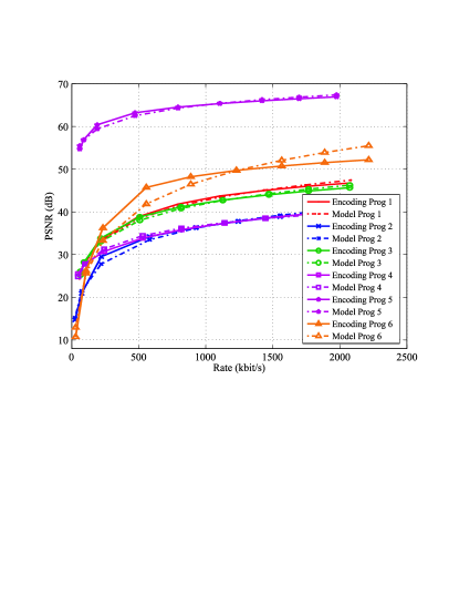
Figure 4: PSNR-rate characteristics and models for the first GoP of the $N=6$ considered programs

An example of the accuracy of the PSNR-rate model (V-C1) is shown in Figure 4, when applied on the first GoP of the six considered programs, with parameters estimated from encoding trials performed at 80 kb/s, 200 kb/s, 800 kb/s, and 2 Mb/s. Figure 4 illustrates the ability of (V-C1) to predict the PSNR over a wide range of rates. In addition, the correlation coefficient $r^{2}$ between experimental and predicted PSNR-rate points is evaluated as

$$r^{2}=\frac{\sigma_{xy}^{2}}{\sigma_{x}^{2}\sigma_{y}^{2}}$$ (38)

with $\sigma_{x}^{2}=\sum_{k=1}^{n}(x_{k}-\bar{x}){}^{2}$, $\sigma_{y}^{2}=\sum_{k=1}^{n}(y_{k}-\bar{y}){}^{2}$, and $\sigma_{xy}^{2}=\sum_{k=1}^{n}(y_{k}-\bar{y})(x_{k}-\bar{x})$, where $n$ is the number of rates for each program at which the PSNR has been evaluated ($x_{k}$) and predicted ($y_{k}$) using (V-C1), and where $\bar{x}$ and $\bar{y}$ are the average values of the $x_{k}$’s and of the $y_{k}$’s. For the six programs, for $n=7$, the rate values are 80 kb/s, 130 kb/s, 200 kb/s, 500 kb/s, 800 kb/s, 1.4 Mb/s, and 2 Mb/s, the correlation coefficients are $r^{2}=[0.998,0.996,0.997,0.996,0.992,0.985]$ illustrating to good fit by (V-C1) of the PSNR-rate characteristics.

V-C2 Controller design and stability analysis

The values of the parameter vector $\boldsymbol{a}_{i}\left(1\right)$, $i=1,\dots,6$, obtained for the first GoP of the $N=6$ programs are

Once $f$ is specified, one may characterize the system equilibrium. The vector of rates at equilibrium $\left(R_{1}^{\text{e,eq}},\dots,R_{N}^{\text{e,eq}}\right)^{T}$ is obtained by solving the system of equations in the state-space representation at equilibrium. $\boldsymbol{\Xi}$ and $\boldsymbol{\Gamma}$ are derived from (29), (30) and (V-C1) as follows

and

$$\boldsymbol{\Gamma}=\text{diag}\left(\frac{a_{1,1}\left(1\right)}{R_{1}^{\text{e,eq}}\left(1\right)},\dots,\frac{a_{N,1}\left(1\right)}{R_{N}^{\text{e,eq}}\left(1\right)}\right).$$ (40)

The gains of the PI controllers have to be chosen so that the roots of

$$d(z)=\det\left(z\mathbf{I}-\mathbf{A}\right)$$ (41)

remains within the unit circle, for various rate-utility characteristics of the VUs. In (41), $\mathbf{A}$ may correspond to $\mathbf{A}^{b}$, the linearized state matrix when considering buffer level control, or to $\mathbf{A}^{\tau}$ with buffering delay control.

To increase the robustness of the proposed approach to variations of the rate-utility characteristics, $K=10$ realizations of $N=4$ random parameter vectors of the PSNR-rate model obtained as follows

$$a_{i,1}^{(k)} =\frac{1}{N}\sum_{i=1}^{N}a_{i,1}\left(1\right)+\eta_{i,1}^{(k)},$$ (42)

$$a_{i,2}^{(k)} =\frac{1}{N}\sum_{i=1}^{N}a_{i,2}\left(1\right)+\eta_{i,2}^{(k)},$$

for $k=1,\dots,K$. In (V-C2), $\eta_{i,1}^{(k)}$ and $\eta_{i,2}^{(k)}$ are realizations of zero-mean Gaussian variables with variance $\sigma_{1}^{2}=6.25\times 10^{-2}$ and $\sigma_{2}^{2}=2.25\times 10^{-4}$. The resulting PSNR-rate characteristics obtained using (V-C2) are represented in Figure 5. These random realizations describe quite well the variability of actual PSNR-rate characteristics represented in Figure 4.

A random search of the control parameters is then performed. Among the values providing stability for the $K$ random PSNR-rate characteristics, the one with the roots farthest away from the unit circle is selected to provide good transients.

The tuning is performed for $N=4$. Good transient behaviors have been obtained with $K_{\text{P}}^{\text{e,b}}=666$, $K_{\text{I}}^{\text{e,b}}=33$, $K_{\text{P}}^{\text{t}}=66\times 10^{3}$, and $K_{\text{I}}^{\text{t}}=1300$.

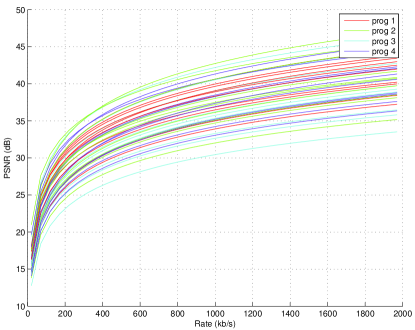
Figure 5: Superposition of the $K=10$ realizations of the $N=4$ random PSNR-rate characteristics

The position of the roots corresponding to the video characteristic represented in Figure 5 are in Figure 6.

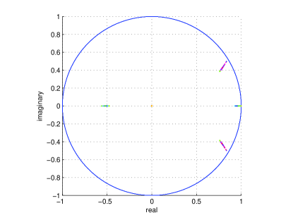
Figure 6: Location of the roots of $\det\left(z\mathbf{I}-\mathbf{A}^{\text{b}}\right)$ for the $K=10$ realizations of the $N=4$ random PSNR-rate characteristics

Figure 6 shows that all roots remain within the unit circle. This result does not prove the robustness of the proposed choice of the control parameters, but shows that this choice leads to a system reasonably robust to changes of the characteristics of the transmitted programs. Nevertheless, some of the roots are located quite near the stability limit, which will lead to quite long transients.

V-C3 Simulation results

The x.264 video encoder is used to perform on-line compression of the different programs with the rate targets provided by the encoding rate controllers. Within the video coder, a two-pass rate control is performed to better fit the target encoding rate. The target and obtained encoding rates may however be slightly different. The system performance is first measured in terms of average buffer level discrepancy $\Delta_{B}$ (in bits) with respect to $B_{0}$, variance of the buffer level $\sigma_{B}^{2}$ (in bits²), PSNR discrepancy $\Delta_{P}$ (in dB), and PSNR variance $\sigma_{P}^{2}$ (in dB²), with

$$\begin{array}[]{l}\Delta_{B}=\frac{1}{NM}\sum_{n=1}^{N}\sum_{l=1}^{M}\left(B_{n}(l)-B_{0}\right),\\ \sigma_{B}^{2}=\frac{1}{N}\sum_{n=1}^{NM}\sum_{l=1}^{M}\left(B_{n}(l)-B_{0}-\Delta_{B}\right)^{2},\\ \Delta_{PSNR}=\frac{1}{NM}\sum_{n=1}^{N}\sum_{l=1}^{M}\left(P_{n}(l)-\bar{P}(l)\right),\\ \sigma_{PSNR}^{2}=\frac{1}{N}\sum_{n=1}^{NM}\sum_{l=1}^{M}\left(P_{n}(l)-\bar{P}(l)-\Delta_{PSNR}\right)^{2},\end{array}$$ (43)

where $\bar{P}(l)=\frac{1}{N}\sum_{n=1}^{N}P_{n}(l)$ and $M$ is the number of GoPs in the video streams.

The results with $N=6$ and $R^{\text{c}}=4$ Mbit/s are summarized in Table II in the three cases: TRF, UMMF, and QF where $\Delta_{B}$ are in kbits and $\sigma_{B}^{2}$ in kbit². The PI controllers used for the transmission rate control loop reduce the PSNR discrepancy between the programs at a price of some increase of the buffer level discrepancy and variance.

	$K_{\text{P}}^{\text{e,b}},K_{\text{I}}^{\text{e,b}}$	$K_{\text{P}}^{t},K_{\text{I}}^{t}$	$\left|\Delta_{B}\right|$	$\sigma_{B}^{2}$	$\left|\Delta_{P}\right|$	$\sigma_{P}^{2}$
TRF	$666,0$	$0,0$	$31.5$	$2.1$	$3.1$	$9.8$
UMMF	$0,0$	$3,0$	$75$	$2$	$2.7$	$13.9$
QF	$666,33$	$(66,1.3)10^{3}$	$53.07$	$6.1$	$1.5$	$6.7$

Table II: Performance when using TRF and QF controllers when controlling the buffer levels for $N=6$.

Figure 7 represents the evolution of the PSNR of the $N$ programs over $300$ GoPs using the TRF (left) and the QF (right) controllers when $N=2$, $N=4$, and $N=6$ with a constant channel rate $R^{\text{c}}=4$ Mbit/s.

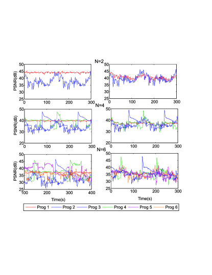
Figure 7: Evolution of the PSNR for $N=2$, $N=4$, and $N=6$ using TRF (left) and QF (right) controllers when controlling the buffer levels

The same controller parameters $K_{\text{P}}^{\text{e,b}}=666$, $K_{\text{I}}^{\text{e,b}}=33$, $K_{\text{P}}^{\text{t}}=66\times 10^{3}$, and $K_{\text{I}}^{\text{t}}=1300$ are used for $N=2$, $N=4$, and $N=6$.

When $N=2$, the average PSNR of Prog $2$, characterized by high activity level, is improved from $36$ dB to $41$ dB, leading to a significant improvement of the video quality. This is at the price of PSNR degradation of Prog $1$, characterized by low activity level, from $45$ dB to $41$ dB. This still corresponds to a very good quality. PSNR fairness improvements are also obtained when $N=4$ and $N=6$.

Figure 8 shows the evolution of the buffer level of the $N$ programs over $300$ GoPs using the TRF (left) and the QF (right) controllers for $N=2$, $N=4$, and $N=6$. The discrepancy between the buffer level and the reference level $B_{0}$ remains limited for most of the time. When only the encoding rate is controlled, corresponding to the TRF controller, the buffer level stabilizes around $B_{0}$.

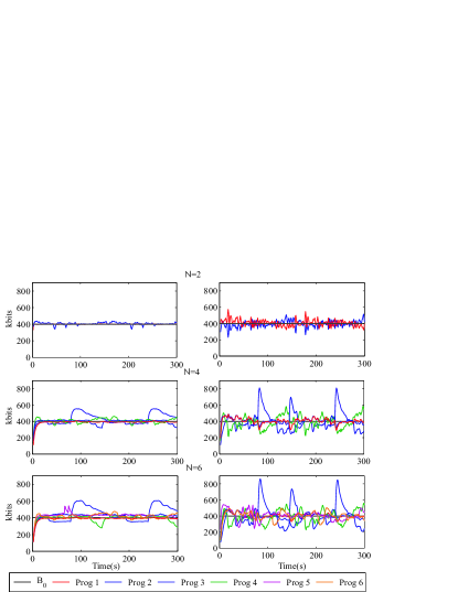
Figure 8: Evolution of the buffer level for $N=2$, $N=4$, and $N=6$ using TRF (left) and QF (right) controllers when controlling the buffer levels

The buffer level variations increase using the QF controller due to the interactions of the encoding rate and transmission rate control loops.

Figure 9 shows the evolution of the buffer level (left) and of the PSNR (right) of the $N$ programs over $300$ GoPs when the UMMF technique is used. The choice of the proportional gain for the transmission rate controller has no significant impact on the quality fairness, provided that the buffers remain full. A reference buffer level of $400$ kbits has been used to allow a satisfying behavior of the transmission rate control loop. The PSNR remains around $40$ dB, but the average variance is of the same order of magnitude as that of the TRF solution, see Table II. This mainly comes from the target encoding rate evaluation on (one step) outdated PSNR-rate characteristics.

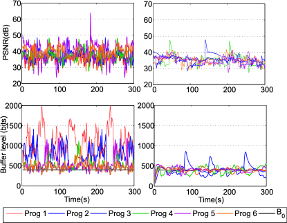
Figure 9: Evolution of the buffer level and of the PSNR (right) for $N=6$ using the UMMF technique (left) and using the QF controllers (right) with a transmission rate control using the buffer levels

V-C4 SSIM-rate model

The quality fairness is also addressed considering the SSIM metric. To tune the PI controllers, an arctan SSIM-Rate utility model is considered

$$U_{i}(j) =S_{i}(j)=f\left(\boldsymbol{a}_{i}\left(j\right),R_{i}^{\text{e}}(j)\right)$$

$$=a_{i}^{(1)}(j)\text{{atan}}(a_{i}^{(2)}(j)R_{i}^{\text{e}}(j))$$

where $S_{i}(j)$ is the SSIM of program $i$ at time $j$. As before, the two entries of each $\boldsymbol{a}_{i}\left(j\right)$ are derived from four encoding trials performed on each of the $N$ considered programs. The resulting values of the parameters are

Figure 10 compares the actual SSIM-Rate characteristics and those obtained using the model (V-C4) for the first GoP of the six considered programs. The model (V-C4) is able to predict accurately the SSIM over a large range of rates. The correlation coefficient for the six programs is $r^{2}=[0.99,0.97,0.99,0.98,0.99,0.99]$ using the same rate values in the PSNR-rate model estimation, which confirms the accuracy of the SSIM-rate model.

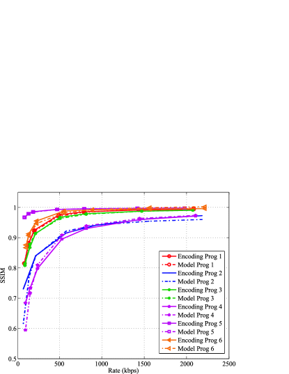
Figure 10: SSIM-Rate model for the six considered programs

Using the SSIM-rate utility function (V-C4), one is able to get the vector $\left(R_{1}^{\text{e,eq}},\dots,R_{N}^{\text{e,eq}}\right)^{T}$ of encoding rates as the solution of (24). $\boldsymbol{\Xi}$ and $\boldsymbol{\Gamma}$ are derived from (29), (30) and (V-C4) as follow

and

$$\boldsymbol{\Gamma}=\text{diag}\left(\begin{array}[]{ccc}\frac{a_{1}^{(1)}a_{1}^{(2)}}{1+(a_{1}^{(2)}R_{1}^{\text{e,eq}})^{2}}&\dots&\frac{a_{N}^{(1)}a_{N}^{(2)}}{1+(a_{N}^{(2)}R_{N}^{\text{e,eq}})^{2}}\end{array}\right)$$ (46)

The choice of the parameters of the controllers is done as in Section V-C2. Good transient behaviors have been obtained with $K_{\text{P}}^{\text{e,b}}=666$, $K_{\text{I}}^{\text{e,b}}=33$, $K_{\text{P}}^{\text{t}}=66\times 10^{4}$, and $K_{\text{I}}^{\text{t}}=1.3\times 10^{4}$.

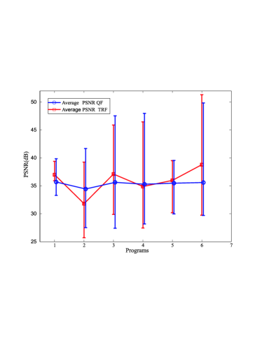
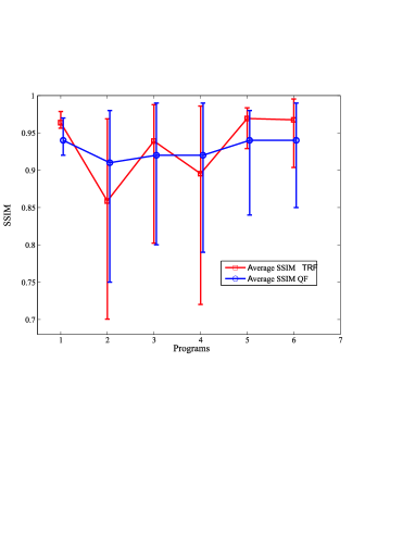
Figure 11: Minimum, average, and maximum values of the PSNR (left) and SSIM (right) over all GoPs for the TRF and the QF controllers using $N=6$ programs when controlling the buffer levels

For this choice of the control gains, Figure 11 shows the minimum, average, and maximum values of the PSNR (left) and SSIM (right) over all GoPs of the $N=6$ programs. The QF controller improves quality fairness especially for the most demanding videos, such as Prog $2$. The proposed QF controller improves also the minimum achieved quality for these programs. In fact, even if events corresponding to these minimum quality happens only few times, the user perception is sometime dominated by the worst experience, rather than the average. The price to be paid is, as expected, a decrease of the quality of the less demanding programs.

V-D Control of the buffering delays

This part focuses on the system performance when the buffering delays are used to evaluate the encoding rates.

V-D1 Controller design

The same PSNR-rate utility model as in (V-C1) is considered in this section. Thus the matrices $\Xi$ and $\boldsymbol{\Gamma}$ are those in (39) and (40).

The choice of the parameters of the two PI controllers is again done as in Section V-C2. Now, the roots of $\det\left(z\mathbf{I}-\mathbf{A}^{\tau}\right)$ have to remain within the unit circle. Good transient behaviors have been obtained for $N=2$, $N=4$, and $N=6$ with $K_{\text{P}}^{\text{t}}=66\times 10^{3}$, $K_{\text{I}}^{\text{t}}=2600$ $K_{\text{P}}^{\text{e}\tau}=66\times 10^{3}$, and $K_{\text{I}}^{\text{e}\tau}=1300$.

In parallel, the parameter $\alpha$ in (9) is tuned to provide the best estimate of the buffering delay. Figure 12 represents the means square error $\text{MSE}(\tilde{\tau},\tau)$ between the actual buffering delay $\tau$ and the estimated one $\tilde{\tau}$ as a function of $\alpha$. The value $\alpha=0.2$ provides the best estimate.

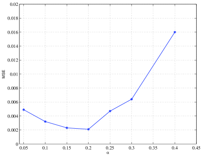
Figure 12: MSE of the estimated buffering delay as a function of $\alpha$.

The evolution with time of the actual buffering delay $\tau$ and of its estimate $\tilde{\tau}$ is represented in Figure 13 for $N=4$ using $\alpha=0.2$ and the QF controller for the PSNR faireness. For this choice of $\alpha$, the estimate provided by (9) for the four video sequences is quite good for most of the time.

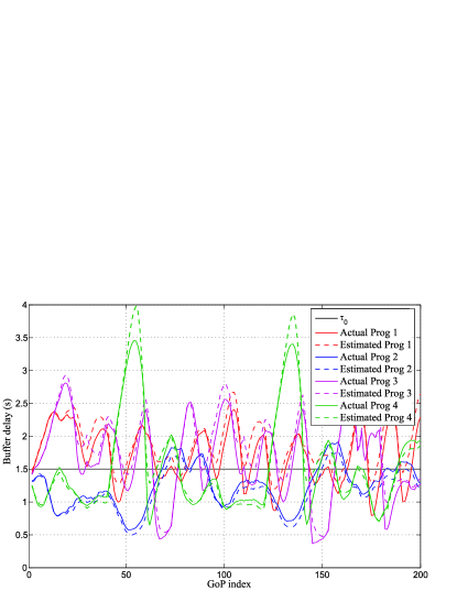
Figure 13: Evolution of the actual buffering delay $\tau$ and of its estimate $\tilde{\tau}$ for $N=4$ using $\alpha=0.2$.

V-D2 Results

The performance of the QF controller using $N=2$, $N=4$, and $N=6$ programs is evaluated in all cases with a transmission rate $R^{\text{c}}=4$ Mps.

We evaluate the PSNR discrepancy $\Delta_{P}$ (in dB) and the PSNR variance $\sigma_{P}^{2}$ (in dB²) defined in (43). Additional performance measures are the average delay discrepancy

$$\Delta_{\tau}=\frac{1}{N}\sum_{n=1}^{N}\left(\frac{1}{M}\sum_{l=1}^{M}\left(\tau_{n}(l)-\tau_{0}\right)\right)$$ (47)

of the buffering delay with respect to $\tau_{0}$ and the variance of the buffering delay

$$\sigma_{\tau}^{2}=\frac{1}{N}\sum_{n=1}^{N}\left(\frac{1}{M}\sum_{l=1}^{M}\left(\tau_{n}(l)-\tau_{0}-\Delta_{\tau}\right)^{2}\right),$$ (48)

where $M$ is the number of GoPs in the video streams. Results with $N=6$ are summarized in Table III in the two cases: QF and TRF controllers.

	$K_{\text{P}}^{\text{e,}\tau},K_{\text{I}}^{\text{e,}\tau}$	$K_{\text{P}}^{\text{t}},K_{\text{I}}^{\text{t}}$	$\Delta_{\tau}$	$\sigma_{\tau}^{2}$	$\Delta_{P}$	$\sigma_{P}^{2}$
TRF	$66\times 10^{3},0$	$0,0$	$0.25$	$0.12$	$3.8$	$10.5$
QF	$66\times 10^{3},1300$	$66\times 10^{3},2600$	$0.6$	$0.35$	$2$	$10$

Table III: Performance of QF and TRF controllers when controlling the buffering delays for $N=6$.

Here again, one notices that using PI controllers for the transmission rate control loop reduces the PSNR discrepancy between the programs at the price of some increase of the buffering delay discrepancy and variance.

Figure 14 represents the evolution of the PSNR when considering the TRF controller (left) and the proposed QF controller (right) $N=2$, $N=4$, and $N=6$ programs. The proposed QF controller reduces the PSNR discrepancy between the $N$ programs compared to the TRF controller. Compared to Figure 7, the control with the buffer level appears to be less reactive. For example, when $N=2$, to improve the PSNR of the second program, the PSNR of the first program has to be decreased. In Figure 7, the PSNRs are almost immediately adjusted. This is done with some delay in Figure 14. This may be due to the difficulty to accurately estimate the buffering delay. A better response could be obtained by increasing $K_{\text{P}}^{\text{e,}\tau}$, which relates the buffering delay and the encoding rate. This, however, would be at the price of a loss in robustness of the global system to variations of the PSNR-rate characteristics of the programs.

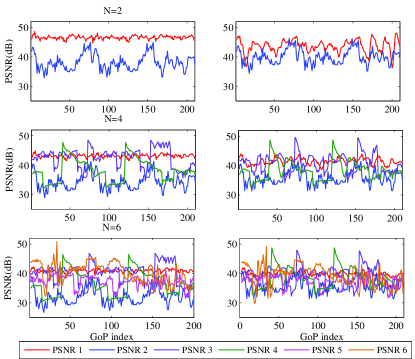
Figure 14: Evolution of the PSNR for $N=2$, $N=4$, and $N=6$ using TRF (left) and QF (right) controllers when controlling the buffer delays.

Figure 15 represents the evolution of the buffering delays of $N$ programs of $300$ GoPs using the TRF (left) and the QF (right) controllers for $N=2$, $N=4$, and $N=6$. With the TRF controller, the buffering delays reach rapidly $\tau_{0}$ and show a reduced variance compared to a system with a QF controller. The larger variations of the buffering delay for the QF controller are due to the interactions of both control loops (encoding rate and transmission rate). Again, $K_{\text{P}}^{\text{e,}\tau}$ appears to be too low: large deviations of the buffering delay are required to reach PSNR fairness.

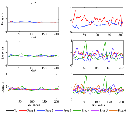
Figure 15: Evolution of the buffering delay for $N=2$, $N=4$, and $N=6$ using TRF (left) and QF (right) controllers when controlling the buffer delays.

V-E Robustness of the proposed solution to variations of the number of users and of the channel rate

In this section, the robustness of the proposed control system (buffering delay control) is evaluated with respect to variations of the channel rate and of the number of transmitted video programs. Similar results are obtained when buffer levels are controlled.

First, the number $N$ of transmitted video programs evolves with time (left). Second, the rate of the channel switches between $R^{c}=3.5$ Mbits/s and $R^{c}=5$ Mbits/s (right), see Figure 16. The PSNR is used as quality measure. When a new video program is transmitted, initially, it has no transmission rate allocated by the MANE (since at time $j$ the controller derives the encoding rate for time $j+1$). Thus, we choose to set the encoding rate at that time as $R^{\text{c}}/N$. In Figure 16 (left), Prog $4$ is not transmitted between GoP $35$ and $65$. The same values for the gains of the PI controllers are used here as in Section V-D.

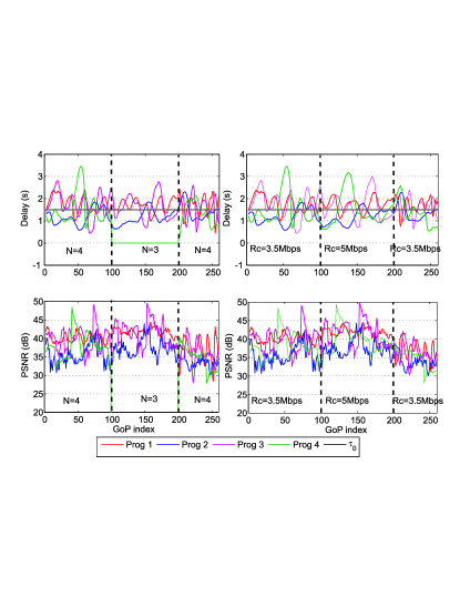
Figure 16: System performance using PI controllers while multiplexing four video programs using the proposed QF controller when considering variations of the channel rate (left) and of the number of programs (right).

When the channel rate increases or when a video program is no more transmitted, the bandwidth allocation adapts rapidly to this change by providing more rate to programs with low video quality (here Prog $2$). When the channel rate decreases or when a new video program is transmitted, the bandwidth allocation performs well, showing the robustness of the proposed control system to variations of the channel rate and to the number of transmitted video programs.

VI Conclusions and perspectives

In this paper, we propose encoding and transmission rate controllers for the transmission of several video streams targeting similar video quality between streams as well as efficient control of the buffering delay. The controlled system is modeled with a discrete-time non-linear state-space representation. PI controllers for the transmission rate and the encoding rate control are considered. The delay introduced by the network propagation between the MANE and the encoders is taken into account. This allows to test the stability of the control system in presence of feedback delay. Simulation results show that the quality fairness (measured with PSNR or SSIM) is improved compared to a solution providing an equal transmission rate allocation. Moreover, the jitter of the buffering delay remains reasonable. The robustness to variations of the characteristics of the channel and of the number of transmitted programs has been shown experimentally.

Simulations are performed at the GoP granularity. Control at the frame level should be considered, however this may require a better consideration of the communication delay between the MANE and the encoders which may be variable with the time. This would also require to better account for the delay, which significantly impedes the behavior of the global control system, especially when controlling the buffering delay. Tools devoted to the control of time-delay systems may be useful in this context, see, e.g.,[32].

Nesrine Changuel (IEEE S’09 - M’12) received her B.S. degree in 2006 and Eng. degree and M.S. degree in electrical engineering in 2008 from the Ecole Nationale Supérieure d’Electronique et de Radioélectricitée de Grenoble, France. She obtained a PhD degree in Control and Signal Processing in 2011 from the Paris-Sud University, Orsay. She is currently working as a research engineer in Alcatel Lucent Bell Labs. Her current research interests are in the areas of video coding, Statistical multiplexing of video programs, scalable video, Rate and Distortion model, resource allocation and scheduling, Markov decision processes (MDPs), and reinforcement learning. She is a Member of the IEEE.

Bessem Sayadi is a member of technical staff in Multimedia Technology domain at Alcatel-Lucent Bell Labs, France. He is member of Alcatel-Lucent Technical Academy, since 2008. He received M.Sc. (00) and Ph.D. (03) degrees in Control and Signal processing from Supélec, Paris-Sud University, with highest distinction. He worked previously as a postdoctoral fellow in the National Centre for Scientific Research (CNRS), and as a senior researcher engineer in Orange Labs. His main research interests are in the area of broadcast technology (DVB, 3GPP), video coding and transport, and resource allocation algorithms for communication networks. He has authored over 55 publications in journal and conference proceedings and serves as a regular reviewer for several technical journals and conferences. He holds nine patents and has more than twenty patent applications pending in the area of video coding and wireless communications.

Michel Kieffer (IEEE M’02 - SM’07) received in 1995 the Agrégation in Applied Physics at the Ecole Normale Supérieure de Cachan. He obtained a PhD degree in Control and Signal Processing in 1999, and the Habilitation à Diriger des Recherches degree in 2005, both from the Paris-Sud University, Orsay. Michel Kieffer is a full professor in signal processing for communications at the Paris-Sud University and a researcher at the Laboratoire des Signaux et Systèmes, Gif-sur-Yvette. Since 2009, he is also invited professor at the Laboratoire Traitement et Communication de l’Information, Télécom ParisTech, Paris. His research interests are in signal processing for multimedia, communications, and networking, distributed source coding, network coding, joint source-channel coding and decoding techniques, joint source-network coding. Applications are mainly in the reliable delivery of multimedia contents over wireless channels. He is also interested in guaranteed and robust parameter and state bounding for systems described by non-linear models in a bounded-error context. Michel Kieffer is co-author of more than 120 contributions in journals, conference proceedings, or books. He is one of the co-author of the book Applied Interval Analysis published by Springer-Verlag in 2001 and of the book Joint source-channel decoding: A crosslayer perspective with applications in video broadcasting published by Academic Press in 2009. He is associate editor of Signal Processing since 2008, of the Journal of Communication and Information Systems since 2011 and of the IEEE Transactions on Communications since 2012. In 2011, Michel Kieffer became junior member of the Institut Universitaire de France.

References

- [1] “Cisco visual networking index: Forecast and methodology, 2008-2013,” Tech. Rep., Cisco, 2009.
- [2] Z. Wang, A.C. Bovik, H.R. Sheikh, and E.P. Simoncelli, “Image quality assessment: from error visibility to structural similarity,” IEEE Transactions on Image Processing, vol. 13, no. 4, pp. 600 – 612, April 2004.
- [3] Z.L. Zhang, S. Nelakuditi, R. Aggarwal, and R.P. Tsang, “Efficient selective frame discard algorithms for stored video delivery across resource constrained networks,” Real-Time Imaging, vol. 7, no. 3, pp. 255 – 273, March 2001.
- [4] T-L. Lin, Y. Zhi, S. Kanumuri, P.C. Cosman, and A.R. Reibman, “Perceptual quality based packet dropping for generalized video gop structures,” in IEEE International Conference on Acoustics, Speech and Signal Processing, April 2009, pp. 781 – 784.
- [5] S. Ma, W. Gao, and Y. Lu, “Rate-distortion analysis for H.264/AVC video coding and its application to rate control,” IEEE Transactions on Circuits and Systems for Video Technology, vol. 15, no. 12, pp. 1533 – 1544, December 2005.
- [6] Z. He and D. O. Wu, “Linear rate control and optimum statistical multiplexing for H.264 video broadcast,” IEEE Transactions on Multimedia, vol. 10, no. 7, pp. 1237 – 1249, November 2008.
- [7] S. K. Srinivasan, J. Vahabzadeh-Hagh, and M. Reisslein, “The effects of priority levels and buffering on the statistical multiplexing of single-layer H.264/AVC and SVC encoded video streams,” IEEE Transactions on Broadcasting, vol. 56, no. 3, pp. 281 – 287, September 2010.
- [8] E. Maani and A.K. Katsaggelos, “Unequal error protection for robust streaming of scalable video over packet lossy networks,” IEEE Transactions on Circuits and Systems for Video Technology, vol. 20, no. 3, pp. 407 – 416, March 2010.
- [9] Y. Li, Z. Li, M. Chiang, and A.R. Calderbank, “Content-aware distortion-fair video streaming in congested networks,” IEEE Transactions on Multimedia, vol. 11, no. 6, pp. 1182 –1193, October 2009.
- [10] N. Changuel, B. Sayadi, and M. Kieffer, “Joint encoder and buffer control for statistical multiplexing of multimedia contents,” in IEEE Globecom, December 2010, pp. 1 – 6.
- [11] C.W Wong, O.C. Au, and H.K. Lam, “PID-based real-time rate control,” in IEEE International Conference on Multimedia and Expo, June 2004, vol. 1, pp. 221 – 224.
- [12] Z. Guo and R. Rojas-Cessa, “Analysis of a flow control system for a combined input-crosspoint buffered packet switch,” in Workshop on High Performance Switching and Routing, May 2005, pp. 336 – 340.
- [13] Y-H. Zhang, K.H Li, C.Q. Xu, and L.M. Sun, “Joint rate allocation and buffer management for robust transmission of VBR video,” Acta Automatica Sinica, vol. 34, no. 3, pp. 1 – 7, March 2008.
- [14] Y. Huang, S. Mao, and S.F. Midkiff, “A control-theoretic approach to rate control for streaming videos,” IEEE Transactions on Multimedia, vol. 11, no. 6, pp. 1072 –1081, October 2009.
- [15] Y. Huang and S. Mao, “Analysis and design of a proportional-integral rate controller for streaming videos,” in IEEE Globecom, November 2009, pp. 5530 – 5535.
- [16] Y. Zhou, Y. Sun, Z. Feng, and S. Sun, “PID-based bit allocation strategy for h.264/avc rate control,” IEEE Transactions on Circuits and Systems II: Express Briefs, vol. 58, no. 3, pp. 184 – 188, March 2011.
- [17] J.W Cho and S. Chong, “Utility max-min flow control using slope-restricted utility functions,” in IEEE Globecom, December 2005, vol. 2, pp. 818 – 824.
- [18] S. Cicalo and V. Tralli, “Cross-layer algorithms for distortion-fair scalable video delivery over OFDMA wireless systems,” in IEEE Globecom Workshops, 2012, pp. 1287 – 1292.
- [19] E. Witrant, C. Canudas-de Wit, D. Georges, and M. Alamir, “Remote stabilization via communication networks with a distributed control law,” IEEE Transactions on Automatic Control, vol. 52, no. 8, pp. 1480 – 1485, August 2007.
- [20] Motorola, “Statistical multiplexing over IP StatmuxIP solution,” Tech. Rep., Motorola, 2009, XP002565902.
- [21] Harmonic, “IP-based distributed statistical multiplexing solution,” Tech. Rep., 2011.
- [22] N. Changuel, B. Sayadi, and M. Kieffer, “Control of distributed servers for quality-fair delivery of multiple video streams,” in ACM international conference on Multimedia, October 2012, pp. 269 – 278.
- [23] K. Seshadrinathan, R. Soundararajan, A.C. Bovik, and L.K. Cormack, “Study of subjective and objective quality assessment of video,” IEEE Transactions on Image Processing, vol. 19, no. 6, pp. 1427 – 1441, June 2010.
- [24] T. Wiegand, H. Schwarz, A. Joch, F. Kossentini, and G.J. Sullivan, “Rate-constrained coder control and comparison of video coding standards,” IEEE Transactions on Circuits and Systems for Video Technology, vol. 13, no. 7, pp. 688 – 703, July 2003.
- [25] K.-B. Kim and H.-J. Kim, “Back-pressure buffering scheme to improve the cell loss property on the output buffered atm switch,” in IEEE Conference on Local Computer Networks, October 1996, pp. 242 – 248.
- [26] ETSI, “Multimedia Broadcast/Multicast service. (MBMS); UTRAN/GERAN requirements,” Tech. Rep., 3GPP TR 25.992-140, 2005.
- [27] V. Vukadinovic and J. Huschke, “Statistical multiplexing gains of H.264/AVC video in E-MBMS,” in International Symposium on Wireless Pervasive Computing, May 2008, pp. 468 – 474.
- [28] x264 Home Page, “Videolan organization. retrieved 2011-03-11.,” 2011.
- [29] ffmpeg Documentation, “http://ffmpeg.org/ffmpeg.html,” .
- [30] Association of Radio Industries and Businesses, “Multimedia Broadcast/Multicast Service (MBMS) user services stage 1 (release 8),” Tech. Rep., 3GPP TS, 2008.
- [31] X. Zhu, P. Agrawal, J. Pal Singh, T. Alpcan, and B. Girod, “Rate allocation for multi-user video streaming over heterogenous access networks,” in ACM Multimedia, Augsburg, September 2007, pp. 37 – 46.
- [32] W. Michiels and S.L. Niculescu, Stability and Stabilization of Time-Delay Systems: An Eigenvalue-Based Approach, Society for Industrial & Applied Mathematics,U.S., 2007.