Hopfions interaction from the viewpoint of the product ansatz

Abstract

We discuss the relation between the solutions of the Skyrme model of lower degrees and the corresponding axially symmetric Hopfions which is given by the projection onto the coset space $SU(2)/U(1)$. The interaction energy of the Hopfions is evaluated directly from the product ansatz. Our results show that if the separation between the constituents is not very small, the product ansatz can be considered as a relatively good approximation to the general pattern of the charge one Hopfions interaction both in repulsive and attractive channel.

1 Introduction

Spatially localized particle-like non-perturbative soliton field configurations have a number of applications in a wide variety of physical systems, from modern cosmology and quantum field theory to condensed matter physics. The study of the interaction between the solitons and their dynamical properties has attracted a lot of attention in many different contexts (for a general review see e.g. [1]). One of these interesting contexts include investigation of a new family of materials known as topological insulators, which also makes relevant the basis research involving topological solitons. Perhaps the most interesting possibility is the discovery that frustrated magnetic materials may support topological insulator phases, for which wave functions are classified by the Hopf invariant [2].

Simple example of topological soliton solutions is given by the class of scalar models from the Skyrme family, the original Skyrme model [3], the Faddeev-Skyrme model [4] in $d=3+1$, and the low-dimensional baby Skyrme model in $2+1$ dimensions [5]. The Lagrangian of all these models as they were formulated originally, has similar structure, it includes the usual sigma-model kinetic term, the Skyrme term, which is quartic in derivatives, and the potential term which does not contain the derivatives. According to the Derrick’s theorem [6], the latter term is optional in $d=3+1$, however it is necessary to stabilise the soliton configurations in the baby-Skyrme model.

A peculiar feature of these models is that the corresponding soliton solutions, Skyrmions and Hopfions, do not saturate the topological bound. In order to attain the topological lower bound and get a relation between the masses of the solitons and their topological charges $Q$, one has to modify the model, for example drop out the quadratic kinetic term [7, 8] or extend the model by coupling of the Skyrmions to an infinite tower of vector mesons [9]. Thus, the powerful methods of differential geometry cannot be directly applied to describe low-energy dynamics of the Skyrmions and Hopfions, one has to analyse the processes of their scattering, radiation and annihilation numerically [15, 16]. Interestingly, the numerical simulations of the head-on collision of the charge one Skyrmions reveal the celebrated picture of the $\pi/2$ scattering through the intermediate axially-symmetric charge two Skyrmion [16], which is typical for BPS configurations like vortices or monopoles (see [1]). The same pattern was observed in the baby Skyrme model using the collective coordinate method [11]. However recent attempt to model the Hopfion dynamics [20] failed to find the channel of right-angle scattering in head-on collisions.

Typically, the problem of direct simulation of the soliton dynamics is related with sophisticated numerical methods, the calculations require considerable amount of computational resources, actually this problem is fully investigated only for the low-dimensional baby Skyrme model. Even more simple task of full numerical investigation of the spinning solitons beyond rigid body approximation was performed only recently in the Faddeev-Skyrme model [22, 23] and in the baby Skyrme model [24, 25], in the case of the original Skyrme model in $d=3+1$ this problem is not investigated yet.

Alternatively, one can delve into the assumptions about the character of the soliton interaction by analogy with the dynamical properties of the Bogomol’nyi type solitons [10, 11, 12]. Then the moduli space approximation for low-energy soliton dynamics can be applied. This approach works especially well for low-dimensional baby Skyrme model because it can be considered as a deformation of the $O(3)$ sigma model. It also explains the observations of the right-angle scattering in the head-on collisions of the Skyrmions in $d=3+1$, however the question about validity of the moduli approximation to the low-energy dynamics of the Hopfions is not quite clear.

Another approach to the problem of interaction between the solitons is to consider the asymptotic field of the configurations, then for example the Skyrmions can be treated as triplets of scalar dipoles [12, 13, 14]. Similarly, the asymptotic fields both the baby Skyrmion and the Hopfion in the sector of degree one correspond to a doublet of orthogonal dipoles [15, 17, 18]. Considering this system Ward predicted existence of three attractive channels in the interaction of the charge one Hopfions with different orientation [18]. It was suggested recently to use a simplified dipole-dipole picture of the interaction between the baby Skyrmions in the ”easy plane” model, thus in this description the interaction energy depends only on the average orientation of the dipoles [19].

In his pioneering paper [3] Skyrme suggested to apply the product ansatz which yields a good approximation to a configuration of well-separated unit charge Skyrmions. The ansatz is constructed by the multiplication of individual Skyrmion fields, besides the rational map ansatz [27] it can be used to produce an initial multi-Skyrmion configuration for consequent numerical calculations [29].

In a similar way one can construct a system of well-separated baby-Skyrmions using the parametrization of the scalar triplet in terms of the $SU(2)$-valued hermitian matrix fields [26]. Evidently, the same approach can be used to model the configuration of well separated static Hopfions of degree one. On the other hand the product ansatz can be applied in the Faddeev-Skyrme model to approximate various multicomponent configurations whose position curve consists of a few disjoint loops, like the $Q=4$ soliton.

In this Letter we discuss the relation between the solutions of the Skyrme model of lower degree and the corresponding axially symmetric Hopfions which is given by the projection onto the coset space $SU(2)/U(1)$. Using this approach we construct the product ansatz of two well-separated single Hopfion configurations. We confirm that the product ansatz correctly reproduces the channels of interaction. Indeed, it is known that similar with the case of the Skyrmions, the interaction between the two Hopfions can be repulsive or attractive depending upon the relative orientation of the solitons [18].

2 The model

Let us consider a Faddeev-Skyrme model Lagrangian in 3+1 dimensions with metric $(+,-,-,-)$:

$${\cal L}=\frac{1}{32\pi^{2}}\left(\partial_{\mu}\phi^{a}\partial^{\mu}\phi^{a}-\frac{1}{4}(\varepsilon_{abc}\phi^{a}\partial_{\mu}\phi^{b}\partial_{\nu}\phi^{c})^{2}\right)\,.$$ (1)

Here $\phi^{a}=(\phi^{1},\phi^{2},\phi^{3})$ denotes a triplet of scalar real fields which satisfy the constraint $|\phi^{a}|^{2}=1$. The finite energy configurations should approach a constant value at spatial infinity, which we selected to be $\phi^{a}(\infty)=(0,0,1)$. Thus, the static field $\mathbf{\phi}(\mathbf{x})$ defines a map $R^{3}\rightarrow S^{2}$, which can be characterized by Hopf invariant $Q=\pi_{3}(S^{2})=\mathbb{Z}$. Then the finite energy solutions of the model, the Hopfions, are the map $S^{3}\to S^{2}$ and the target space $S^{2}$ by construction is the coset space $SU(2)/U(1)$.

It follows that any coset space element $\mathbf{H}$ can be projected from generic $SU(2)$ group element $\mathbf{U}$. In circular coordinate system the projection can be written in the following form,

$$\mathbf{H}=2\sum_{a}(-1)^{a}\tau_{a}\phi_{-a}=2\mathbf{U}\tau_{0}\mathbf{U}^{\dagger}\,,$$ (2)

where the Pauli matrices $(\tau_{1},\tau_{0},\tau_{-1})$ are chosen to satisfy relation

$$\tau_{a}\tau_{b}=\frac{1}{4}(-1)^{a}\delta_{a,-b}\mathbf{1}-\frac{1}{\sqrt{2}}\left[\begin{matrix}1&1&1\\ a&b&c\end{matrix}\right]\tau_{c},$$ (3)

and $\left[\begin{smallmatrix}1&1&1\\ a&b&c\end{smallmatrix}\right]$ denotes the Clebsch-Gordon coefficient. It is convenient to rewrite the Lagrangian (1) directly in terms of coset space elements $\mathbf{H}$,

$${\cal L}=\frac{1}{64\pi^{2}}\left({\rm Tr}\big{\{}\partial_{\mu}\mathbf{H}\partial^{\mu}\mathbf{H}\big{\}}+\frac{1}{16}{\rm Tr}\big{\{}\bigl{[}\partial_{\mu}\mathbf{H},\partial_{\nu}\mathbf{H}\bigr{]}\bigl{[}\partial^{\mu}\mathbf{H},\partial^{\nu}\mathbf{H}\bigr{]}\big{\}}\right)\,.$$ (4)

The difference between the Skyrmions and Hopfions is that in the latter case the dimensions of the domain space and the target space are not the same, the topological charge of the Hopfions is not defined locally. It has a meaning of the linking number in the domain space [4].

There have been many investigations of the solutions of the model (1) [17, 28, 29, 30]. Here we restrict out consideration to the axially symmetric configurations of lower degrees $Q=1,2$ which are conventionally labeled as ${\cal A}_{1,1}$ and ${\cal A}_{2,1}$ [28].

An approximation to these solutions can be constructed via Hopf projection of the corresponding Skyrmion configurations with baryon numbers $B=1$ and $B=2$, respectively. Indeed, it have been shown [29, 31] that up to a constant, the solution for the charge $Q=1$ Hopfion can be written in a form which is equivalent to the standard hedgehog solution of the Skyrme model with the usual profile function $F(r)$. This construction yields the hopfion with mass $1.232$. In our conventions  (4) the ${\cal A}_{1,1}$ configuration is $\mathbf{H}_{1}$ which is a projection of the Skyrmion matrix valued field $\mathbf{U}_{0}$, i.e.

$$\mathbf{H}_{1}(\mathbf{r})=2\mathbf{U}_{0}(\mathbf{r})\tau_{0}\mathbf{U}_{0}^{\dagger}(\mathbf{r})\,,$$ (5)

where $\mathbf{U}_{0}(\mathbf{r})$ denotes the usual spherically symmetric Skyrmion which is parametrised via the hedgehog ansatz

$$\mathbf{U}_{0}(\mathbf{r})=\exp\bigl{(}2\mathrm{i}(\hat{\mathbf{r}}\cdot\boldsymbol{\tau})F(r)\bigr{)}\,.$$ (6)

Here $\hat{\mathbf{r}}$ denotes the unit position vector and $F(r)$ is a monotonically decreasing profile function of the Skyrmion with usual boundary conditions, $F(0)=0,\leavevmode\nobreak\ \leavevmode\nobreak\ F(\infty)=\pi$.

In terms of the triplet scalar fields $\phi_{a}$ in the circular coordinate system defined by $\phi_{\pm 1}=\mp\frac{1}{\sqrt{2}}\bigl{(}\phi^{1}\pm\mathrm{i}\phi^{2}\bigr{)}$ and $\phi_{0}=\phi^{3}$, the projected Skyrme configuration can be written as

$$\phi_{a}=2\sin^{2}F(r)\hat{r}_{0}\hat{r}_{a}+\mathrm{i}a\sin\bigl{(}2F(r)\bigr{)}\hat{r}_{a}+\cos\bigl{(}2F(r)\bigr{)}\delta_{0,a}\,.$$ (7)

Evidently, although the ansatz  (6) depends on the radial variable only, expression (7) clearly demonstrates, that the corresponding ${\cal A}_{1,1}$ Hopfion does not possess the spherical symmetry, the projection breaks it down to axial symmetry [29].

The residual $O(2)$ symmetry of global rotations by the phase $\alpha$ around the third axis in the internal space changes the triplet in the following way

$$\phi_{+1}\rightarrow\phi_{+1}\mathrm{e}^{i\alpha},\quad\phi_{-1}\rightarrow\phi_{-1}\mathrm{e}^{-i\alpha},\quad\phi_{0}\rightarrow\phi_{0}\,.$$ (8)

Remind that in the case of the hedgehog ansatz the iso-rotation of the configuration is equivalent to rotation of the vector $\hat{r}_{a}$ by angle $\alpha$ around the $z$-axis.

The position curve of Hopfion is a is commonly chosen to be the curve $\phi^{-1}(0,0,-1)$, the preimage of the point $(0,0,-1)$ which is the antipodal to the vacuum $(0,0,1)$. For the simplest ${\cal A}_{1,1}$ Hopfion this is a circle of radius $F(r_{c})=\pi/2$, with numerical value $r_{c}=0.8763$ in the $x-y$ plane. Small deviations $F(r)=F(r_{0})+\epsilon$ then define the tube around the position curve where $\vartheta\approx\pi/2$ and $\varphi=[0,2\pi)$.

From the parametrization (7) we can define the orientation of the single Hopfion. Indeed, a clockwise rotation by an angle $\varphi$ in equatorial plane corresponds to a counterclockwise rotation of the tube point on the target space

$$\phi^{1}\approx 2\epsilon\sin\varphi,$$ (9a)

$$\phi^{2}\approx -2\epsilon\cos\varphi,$$ (9b)

$$\phi^{3}\approx -1.$$ (9c)

Here, for the sake of convenience, we are using the component notations of the field $\phi$.

Note that the Hopfion charge can be inverted by the transformation $\mathbf{H}\rightarrow\mathbf{H}^{*}$ or $\phi_{a}\rightarrow(-1)^{a}\phi_{-a}$. It is easy to see that in this case the signs of the right hand sides of (9a) and (9b) are inverted, thus a clockwise rotation about the $z$ axis in the domain space corresponds to a clockwise rotation on the target space. So for the Hopfion with negative topological charge the point on the tube rotates in the opposite direction. Thereafter we restrict our investigation to the case of positive values of $Q$ only.

For single Hopfion we can rotate the points on the tube by applying rotation transform via the $SU(2)$ matrix

$$\mathbf{H}\rightarrow D(\alpha)\mathbf{H}D(-\alpha)\,.$$ (10)

Evidently this transformation is equivalent to (8) and it leaves invariant the Lagrangian (4).

Let us now consider two identical Hopfions of degree one which are placed at the points $\mathbf{R}/2$ and $-\mathbf{R}/2$ and separated by a distance $R$, as shown in Fig. 1. There the polar angle $\Theta$ yields the orientation of the Hopfions relative to the $z$-axis. Note that in this frame the pattern of interaction is invariant with respect to the spacial rotations of the system around the $z$-axis by an azimuthal angle $\Phi$.

Figure 1: Geometry of the system of two interacting Hopfions $h_{1}$ and $h_{2}$, placed at the points $\mathbf{R}/2$ and $-\mathbf{R}/2$, respectively.

First, we suppose that both separated Hopfions are counterclockwise oriented and they are in phase, i.e. $\Delta\alpha=0$. This system can be approximated by the product ansatz

$$\mathbf{H}_{2}^{\Delta\alpha=0}(\mathbf{r})=2\mathbf{U}_{0}(\mathbf{r}^{\prime})\mathbf{U}_{0}(\mathbf{r}^{\prime\prime})\tau_{0}\mathbf{U}_{0}^{\dagger}(\mathbf{r}^{\prime\prime})\mathbf{U}_{0}^{\dagger}(\mathbf{r}^{\prime})\,$$ (11)

where $\mathbf{r}^{\prime}=\mathbf{r}+\mathbf{R}/2$ and $\mathbf{r}^{\prime\prime}=\mathbf{r}-\mathbf{R}/2$.

Here fields of both Hopfions at the spacial boundary tend to the same asymptotics $(0,0,1)$. Note, however, that in the constituent system (11) of two identical Hopfions of degree one, contrary to the single Hopfion case, the transformation (10) of one of the Hopfions $\mathbf{H}$ do not leave the Lagrangian (4) invariant, it becomes a function of relative phase difference $\alpha$.

Further, in addition to the ansatz (11) we can consider two separated Hopfions of degree one with opposite phases, $\Delta\alpha=\pi$. Using the definition (6) we can express this system in terms of the matrix $\mathbf{U}_{0}(\mathbf{r})$, thus the corresponding product ansatz is different from (11):

$$\begin{split}\mathbf{H}_{2}^{\Delta\alpha=\pi}(\mathbf{r})=8\mathbf{U}_{0}(\mathbf{r}^{\prime})\tau_{0}\mathbf{U}_{0}(\mathbf{r}^{\prime\prime})\tau_{0}\mathbf{U}_{0}^{\dagger}(\mathbf{r}^{\prime\prime})\tau_{0}\mathbf{U}_{0}^{\dagger}(\mathbf{r}^{\prime})\,,\end{split}$$ (12)

An advantage of the product ansatz approximations (11) and (12) is that it ensures the conservation of the total topological charge for any separation $R$ and space orientation of the constituents. The simple additive ansatz of two unit charge Hopfions used by Ward [18] to construct the Hopfion of degree two can be considered as a good approximation only if the Hopfions are well separated.

Substitution of product ansatzes (11) and (12) into Lagrangian (4) allows us to write down the expressions for the corresponding energy densities of both configurations as a function of the components of the position vectors $r_{i}^{\prime}$ and $r_{j}^{\prime\prime}$ (cf Fig. 1).

Using the Gröebner basis method implemented in Mathematica, we can collect these components into various combinations. It appears that in all cases the expressions for the local energy, as well as for the corresponding topological charge density are some functions only of the distances $r^{\prime}$ and $r^{\prime\prime}$, the dot product $\mathbf{r}^{\prime}\cdot\mathbf{r}^{\prime\prime}$, $z$-components of the vectors $r_{0}^{\prime}$, $r_{0}^{\prime\prime}$ and the cross product $(\mathbf{r}^{\prime}\times\mathbf{r}^{\prime\prime})_{0}$.

Let us now express these quantities in terms of the Hopfion’s position coordinates $R,\Theta,\Phi$ and the spherical coordinates $r,\theta,\varphi$, then the numerical integration of the corresponding local densities over the variables $\varphi,\vartheta$ and $r$ yields the total energy (mass) of the system and its topological charge. In order to do it we apply some useful identities:

$$r^{\prime}= \bigl{(}r^{2}+R^{2}/4+rR(\cos\Theta\cos\vartheta+\sin\Theta\sin\vartheta\cos(\varphi-\Phi))\bigr{)}^{1/2},$$

$$r^{\prime\prime}= \bigl{(}r^{2}+R^{2}/4-rR(\cos\Theta\cos\vartheta+\sin\Theta\sin\vartheta\cos(\varphi-\Phi))\bigr{)}^{1/2},$$

$$(\mathbf{r}^{\prime}\times\mathbf{r}^{\prime\prime})_{0}= \frac{rR\sin\Theta\sin\vartheta\sin(\Phi-\varphi)}{r^{\prime}r^{\prime\prime}},$$

$$(\mathbf{r}^{\prime}\cdot\mathbf{r}^{\prime\prime})= \frac{r^{2}-(R^{2}/4)}{r^{\prime}r^{\prime\prime}},$$ (13)

$$r^{\prime}_{0}= \frac{r\cos\vartheta+(R/2)\cos\Theta}{r^{\prime}},$$

$$r^{\prime\prime}_{0}= \frac{r\cos\vartheta-(R/2)\cos\Theta}{r^{\prime\prime}}\,.$$

Now, we illustrate the calculation procedure on a particular example of evaluation of the local topological charge density, which in the circular coordinates is

$$\begin{split}{\cal Q}(\mathbf{r}^{\prime},\mathbf{r}^{\prime\prime})=&\mathrm{i}\sqrt{2}(-1)^{a+b}\left[\begin{matrix}1&1&1\\ a&b&a+b\end{matrix}\right]\mathop{\mathrm{Tr}}\Bigl{(}\nabla_{a}\bigl{(}\mathbf{U}_{0}(\mathbf{r}^{\prime})\mathbf{U}_{0}(\mathbf{r}^{\prime\prime})\bigr{)}\mathbf{U}_{0}^{\dagger}(\mathbf{r}^{\prime\prime})\mathbf{U}_{0}^{\dagger}(\mathbf{r}^{\prime})\\ \times&\nabla_{b}\bigl{(}\mathbf{U}_{0}(\mathbf{r}^{\prime})\mathbf{U}_{0}(\mathbf{r}^{\prime\prime})\bigr{)}\mathbf{U}_{0}^{\dagger}(\mathbf{r}^{\prime\prime})\mathbf{U}_{0}^{\dagger}(\mathbf{r}^{\prime})\nabla_{-a-b}\bigl{(}\mathbf{U}_{0}(\mathbf{r}^{\prime})\mathbf{U}_{0}(\mathbf{r}^{\prime\prime})\bigr{)}\mathbf{U}_{0}^{\dagger}(\mathbf{r}^{\prime\prime})\mathbf{U}_{0}^{\dagger}(\mathbf{r}^{\prime})\Bigr{)}\,.\end{split}$$ (14)

Substitution of the product ansatz of two aligned ${\cal A}_{1,1}$ Hopfions (11) into (14) yields the following expression for the topological charge density

$$\begin{split}&{\cal Q}^{\Delta\alpha=0}(\mathbf{r}^{\prime},\mathbf{r}^{\prime\prime})=-6\biggl{(}(1-(\mathbf{r}^{\prime}\cdot\mathbf{r}^{\prime\prime})^{2})F^{\prime}(r^{\prime})F^{\prime}(r^{\prime\prime})\Bigl{(}\frac{\sin(2F(r^{\prime}))}{r^{\prime}}+\frac{\sin(2F(r^{\prime\prime}))}{r^{\prime\prime}}\Bigr{)}\\ &+\frac{2\sin^{2}F(r^{\prime})}{r^{\prime 2}}\Bigl{(}F^{\prime}(r^{\prime\prime})(\mathbf{r}^{\prime}\cdot\mathbf{r}^{\prime\prime})^{2}+F^{\prime}(r^{\prime})\Bigr{)}+\frac{2\sin^{2}F(r^{\prime\prime})}{r^{\prime\prime 2}}\Bigl{(}F^{\prime}(r^{\prime})(\mathbf{r}^{\prime}\cdot\mathbf{r}^{\prime\prime})^{2}+F^{\prime}(r^{\prime\prime})\Bigr{)}\\ &+\frac{(1-(\mathbf{r}^{\prime}\cdot\mathbf{r}^{\prime\prime})^{2})}{r^{\prime}r^{\prime\prime}}\Bigl{(}\frac{\sin(2F(r^{\prime}))\sin^{2}F(r^{\prime\prime})}{r^{\prime\prime}}\Bigr{)}+\frac{\sin^{2}F(r^{\prime})\sin(2F(r^{\prime\prime}))}{r^{\prime}}\\ &+\frac{2\sin F(r^{\prime})\sin F(r^{\prime\prime})\bigl{(}F^{\prime}(r^{\prime})+F^{\prime}(r^{\prime\prime})\bigr{)}}{r^{\prime}r^{\prime\prime}}\Bigl{(}-2\sin F(r^{\prime})\sin F(r^{\prime\prime})(\mathbf{r}^{\prime}\cdot\mathbf{r}^{\prime\prime})\\ &+(1+(\mathbf{r}^{\prime}\cdot\mathbf{r}^{\prime\prime})^{2})\cos F(r^{\prime})\cos F(r^{\prime\prime})\Bigr{)}\biggr{)}\,.\end{split}$$ (15)

It is possible to compute the total topological charge of the configuration to verify our construction for correctness. This task becomes a little bit more simple since the expression (15) depends only on the variables $r^{\prime}$, $r^{\prime\prime}$ and the dot product $(\mathbf{r}^{\prime}\cdot\mathbf{r}^{\prime\prime})$. If we suppose that both Hopfions are sitting on top of each other, i.e. $R\rightarrow 0$, then from (15) and (2) we find

$$\lim_{R\rightarrow 0}{\cal Q}^{\Delta\alpha=0}(\mathbf{r}^{\prime},\mathbf{r}^{\prime\prime})=-\frac{24\sin^{2}\bigl{(}2F(r)\bigr{)}F^{\prime}(r)}{r^{2}}.$$ (16)

Thus, this formula is different from its counterpart for the topological charge one configuration by factor of two. Evidently, the total topological charge of the configuration then can be obtained by evaluation of the integral (15) over the domain

$$Q=\frac{1}{24\pi^{2}}\int_{0}^{2\pi}\mathrm{d}\varphi\int_{0}^{\pi}\mathrm{d}\vartheta\sin\vartheta\int_{0}^{\infty}\mathrm{d}rr^{2}{\cal Q}(\mathbf{r}^{\prime},\mathbf{r}^{\prime\prime})$$ (17)

when the parameters $R$, $\Theta$ and $\Phi$ are arbitrary. Using the above mentioned boundary conditions on the profile function $F(r)$, we arrived at $Q=2$, as expected.

The same procedure can be repeated when the Hopfions are in oposite phase, i.e. for the configuration given by the product anzats (12). In this case, however the corresponding topological charge density depends on the variables $\mathbf{r}_{0}^{\prime}$ and $\mathbf{r}_{0}^{\prime\prime}$ as well as the above mentioned set of variables, thus the result is a bit more complicated than (15) and is not repesented here. Explicitly, in the limit $R\rightarrow 0$ it results in the function of the radial variable $r$ and angle $\theta$ which is different from it counterpart (16) and possesses a double zero at the origin

$$\lim_{R\rightarrow 0}{\cal Q}^{\Delta\alpha=\pi}(\mathbf{r}^{\prime},\mathbf{r}^{\prime\prime})=-\frac{96\cos^{2}\theta\sin^{4}\bigl{(}F(r)\bigr{)}F^{\prime}(r)}{r^{2}}.$$ (18)

However, the integration of this function subject of the same boundary conditions, also gives the same result $Q=2$ for any values of the separation $R$ and orientation angles $\Theta$ and $\Phi$. Thus, we can identify this expression with the topological charge density of the ${\cal A}_{2,1}$ Hopfion.

3 Numerical results

In a general case, evaluation of the total topological charge and the energy of the configuration constructed via a product ansatz needs some numerical computations. In Figs. 2 and 3 the calculated isosurfaces of the topological charge densities are presented for some fixed values of the set of orientation parameters, both for the Hopfions which are in phase and in the opposite phases, i.e. applying the ansatz (11) and (12), respectively. Evidently, if the separation parameter $R$ is not very small, the product ansatz field given by (11),(12) correctly reproduces the familiar structure of the system of two ${\cal A}_{1,1}$ Hopfions. Note that in the first case, as separation parameter $R$ goes to some small but still non-zero value, the axially symmetric charge two ${\cal A}_{1,2}$ unstable configuration of charge two [32] is recovered.

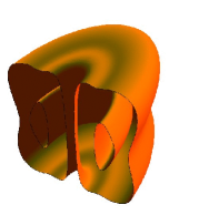
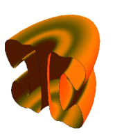
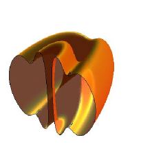
a) b) c) d)

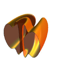
Figure 2: Isosurfaces of the constant topological charge density of the product ansatz Hopfions which are in phase, are presented at ${\cal Q}^{\Delta\alpha=0}(\mathbf{r}^{\prime},\mathbf{r}^{\prime\prime})=0.033$ (a) and ${\cal Q}^{\Delta\alpha=0}(\mathbf{r}^{\prime},\mathbf{r}^{\prime\prime})=0.043$ (b) for the set of orientation parameters $R=1,\Theta=0,\Phi=0$ (upper panel) and $R=1,\Theta=\pi/2,\Phi=0$ (plots (c),(d), bottom panel). The surfaces are clipped through the vertical $\theta-r$ plane.

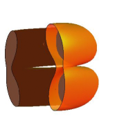
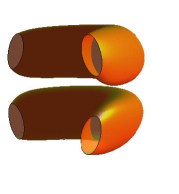
a) b) c)

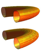
Figure 3: Isosurfaces of the constant topological charge density of the oposite phase product ansatz Hopfions are presented for the set of orientation parameters $R=1,\Theta=\pi/2,\Phi=0$ at ${\cal Q}^{\Delta\alpha=\pi}(\mathbf{r}^{\prime},\mathbf{r}^{\prime\prime})=0.113$ (a), ${\cal Q}^{\Delta\alpha=\pi}(\mathbf{r}^{\prime},\mathbf{r}^{\prime\prime})=0.133$ (b) and for the orientation parameters $R=1,\Theta=0,\Phi=0$ at ${\cal Q}^{\Delta\alpha=\pi}(\mathbf{r}^{\prime},\mathbf{r}^{\prime\prime})=0.113$ (c). The surfaces are clipped through the vertical $\theta-r$ plane.

Let us now evaluate the energy of interaction between the Hopfions. Particularly, for each set of fixed values of the orientation parameters $R$, $\Theta$ and $\Phi$, the integration of the energy density yields the value of the interaction energy of the Hopfions once the masses of two infinitely separated Hopfions (i.e. $M_{0}=2\times 1.232\times 32\pi^{2}$) are subtracted.

We have performed simulations with varying values of the parameters $R$, $\Theta$ and $\Phi$. In Figs. 4,5 we presented the integrated product ansatz interaction energy as a function of the orientation parameters for in phase and oposite phase Hopfions, respectively.

First, from our results we can conclude that the above product ansatz fields, both (11) and (12) correctly reproduce the pattern of interaction between the Hopfions based on the simplified dipole-dipole approximation [18]. Indeed, both for configurations which are in phase and in opposite phases, the orientation along direction given by $\Theta=0$ matches the Channel A discussed by Ward [18]. The orientation angle $\Theta=\pi/2$ corresponds to the Channel B. Note that the Channel C represents the interaction between Hopfion and anti-Hopfion, therefore is out of the scope of the present work. Other values of $\Theta$ correspond to intermediate relative orientations of the Hopfions.

When the Hopfions are in phase and $\Theta=0$ (Channel A) there is a shallow attractive window for separations $R$ large than 4, as can be seen from Fig. 4 (b). Evidently, this attractive channel is very narrow because the potential of interaction quickly becomes repulsive as the value of $\Theta$ increases. Note that the repulsive part of the potential is concentrated inside the core where the product ansatz approximation is not very useful.

If $\Theta=\pi/2$ (i.e. the Hopfions are in side by side position), the interaction potential is always repulsive as displayed in Fig. 4 (c). The energy of interaction for other orientations of the Hopfions is represented by a surface depicted in Fig. 4(a).

The pattern of interaction between the opposite phase ${\cal A}_{1,1}$ Hopfions is rather different. Fig. 5 (b) shows the corresponding energy of interaction as a function of the orientation parameters. Evidently, in contrast with Fig. 4 (b) in the Channel A ($\Theta=0$ ) the interaction is always repulsive for any values of the separation parameter $R$. However, in the Channel B ($\Theta=\pi/2$) the interaction energy is taking relatively large negative value at the separation about the size of the core $r_{c}=0.8763$ and then at gradually approach zero as separation between the Hopfions increases, as shown in Fig. 5 (c).

Finally, in Fig. 5 (a) we depicted the energy of interaction between the Hopfions which are in opposite phases, as function of the orientation parameters $R$ and $\Theta$. We also have checked that the integrated interaction energy does not depend on the azimuthal angle $\Phi$, as expected, though the expressions (2) demonstrate that the energy density functional explicitly depends on this orientation parameter.

To sum up, the product ansatz successfully captures the basic pattern of the interaction between the ${\cal A}_{1,1}$ Hopfions, our calculations suggest that for an arbitrary orientation of the Hopfions the system will evolve towards the state with minimal energy shown in Fig. 5 (c). Qualitatively this conclusion is in agreement with recent results of full 3d numerical simulations of the Hopfions dynamics presented in [20].

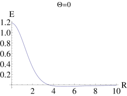
a)
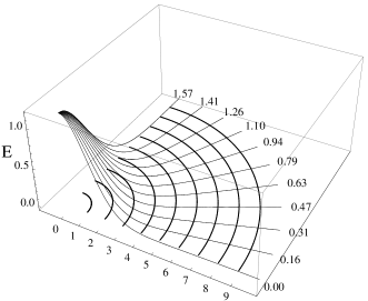
b) c)

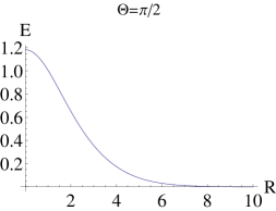
Figure 4: The evaluated interaction energy density of the $\Delta\alpha=0$, product ansatz Hopfions (in phase) as a function of the orientation parameters $R$ and $\Theta$.

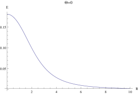
a)
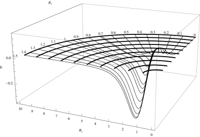
b) c)

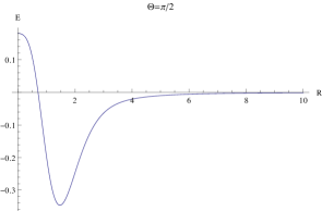
Figure 5: The interaction energy density of the $\Delta\alpha=\pi$, product ansatz Hopfions (opposite phases) as a function of the orientation parameters $R$ and $\Theta$.

Conclusion

Using Hopf projection of the Skyrme field and the product ansatz approximation we have investigated the pattern of interaction between the axially symmetric ${\cal A}_{1,1}$ Hopfions, in particular we analysed how the interaction energy depends on the orientation parameters, the separation $R$ and the polar angle $\Theta$. We have shown that this approach correctly reproduces both the repulsive and attractive interaction channels discussed previously in the limit of the dipole-dipole interactions. Here we mainly restricted our discussion to two most interesting cases considering in phase and oposite phase ${\cal A}_{1,1}$ Hopfions.

Finally, let us note that the product ansatz can be applied to construct a system of interacting Hopfions of higher degrees. It can be done if instead of the Skyrmion matrix valued hedgehog field (6) we project the corresponding rational map Skyrmions [27, 29]. On the other hand, setting the value of the separation parameter $R$ about the size of the core may be used to approximate various linked solitons, for example the configuration ${\cal L}_{1,1,1}^{1,1,1}$ can be constructed as a projection of the product of three matrix valued Skyrme fields (6).

References

- [1] N. Manton and P. Sutcliffe, Topological Solitons, (Cambridge University Press, Cambridge, England, 2004).
- [2] J. E., Moore, Y. Ran and X.-G. Wen, Phys. Rev. Lett. 101 (2008) 186805 [arXiv:0804.4527v2].
- [3] T. H. R. Skyrme, Proc. Roy. Soc. Lond. A 260 (1961) 127.
-
[4]
L.D. Faddeev, Quantization of solitons, Princeton preprint IAS-75-QS70 (1975)
L.D Faddeev and A. Niemi, Nature 387, 58 (1997); Phys. Rev. Lett. 82, 1624 (1999). -
[5]
B.M.A. Piette, W.J. Zakrzewski, H.J.W. Mueller-Kirsten, D.H. Tchrakian,
Phys. Lett. B 320 (1994) 294.
B.M.A. Piette, B.J. Schroers, W.J. Zakrzewski, Z. Phys. C 65 (1995) 165. - [6] G.H. Derrick, J. Math. Phys. 5 (1964) 1252.
- [7] C. Adam, J. Sanchez-Guillen and A. Wereszczynski, Phys. Lett. B 691 (2010) 105 [arXiv:1001.4544 [hep-th]].
- [8] D. Foster, Phys. Rev. D 83 (2011) 085026 [arXiv:1012.2595 [hep-th]].
- [9] P. Sutcliffe, JHEP 1104 (2011) 045 [arXiv:1101.2402 [hep-th]].
- [10] N. S. Manton, Phys. Rev. Lett. 60 (1988) 1916.
- [11] P. M. Sutcliffe, Nonlinearity 4 (1991) 4, 1109.
- [12] B. J. Schroers, Z. Phys. C 61 (1994) 479 [hep-ph/9308236].
- [13] N. S. Manton, Acta Phys. Polon. B 25 (1994) 1757.
- [14] N. S. Manton, B. J. Schroers and M. A. Singer, Commun. Math. Phys. 245 (2004) 123 [hep-th/0212075].
- [15] B. M. A. G. Piette, B. J. Schroers and W. J. Zakrzewski, Nucl. Phys. B 439 (1995) 205 [hep-ph/9410256].
- [16] R. A. Battye and P. M. Sutcliffe, Phys. Lett. B 391 (1997) 150
- [17] J. Gladikowski and M. Hellmund, Phys. Rev. D 56 (1997) 5194 [arXiv:hep-th/9609035].
- [18] R. S. Ward, Phys. Lett. B 473 (2000) 291 [hep-th/0001017].
- [19] J. Jaykka and M. Speight, Phys. Rev. D 82 (2010) 125030 [arXiv:1010.2217 [hep-th]].
- [20] J. Hietarinta, J. Palmu, J. Jaykka and P. Pakkanen, New J. Phys. 14 (2012) 013013 [arXiv:1108.5551 [hep-th]].
- [21] A.F. Vakulenko and L.V. Kapitansky, Sov. Phys. Dokl. 24, 432 (1979).
- [22] R. Battye, M. Haberichter, Phys. Rev. D 87 (2013) 105003 (11pp).
- [23] D. Harland, J. Jäykkä., Ya. Shnir and M. Speight, J. Phys. A: Math. Theor. 46 (2013) 225402 (18pp).
- [24] A. Halavanau and Y. Shnir, Phys. Rev. D 88 (2013) 085028 [arXiv:1309.4318 [hep-th]].
- [25] R. A. Battye and M. Haberichter, Phys. Rev. D 88 (2013) 125016 arXiv:1309.3907 [hep-th].
- [26] A. Acus, E. Norvaisas and Y. Shnir, Phys. Lett. B 682 (2009) 155 [arXiv:0909.5281 [hep-th]].
- [27] C. J. Houghton, N. S. Manton and P. M. Sutcliffe, Nucl. Phys. B 510 (1998) 507 [hep-th/9705151].
- [28] P. Sutcliffe, Proc. Roy. Soc. Lond. A 463 (2007) 3001 [arXiv:0705.1468 [hep-th]].
- [29] R. Battye and P. Sutcliffe, Phys. Rev. Lett. 81 (1998) 4798
- [30] J. Hietarinta and P. Salo, Phys. Rev. D 62 (2000) 081701 .
- [31] Wang-Chang Su, Chin. J. Phys. 40 (2002) 516 [hep-th/0107187].
- [32] J. Hietarinta and P. Salo, Phys. Lett. B 451 (1999) 60 [hep-th/9811053].
- [33] C. J. Houghton, N. S. Manton and P. M. Sutcliffe, Nucl. Phys. B 510 (1998) 507