Stochastic ${\cal PT}$-symmetric coupler

Abstract

We introduce a stochastic ${\cal PT}$-symmetric coupler, which is based on dual-core waveguides with fluctuating parameters, such that the gain and the losses are exactly balanced in average. We consider different parametric regimes which correspond to the broken and unbroken ${\cal PT}$ symmetry, as well as to the exceptional point of the underlying deterministic system. We demonstrate that in all the cases the statistically averaged intensity of the field grows. This result holds for either linear or nonlinear coupler and is independent on the type of fluctuations.

Centro de Física Teórica e Computacional and Departamento de Física, Faculdade de Ciências, Universidade de Lisboa, Avenida Professor Gama Pinto 2, Lisboa 1649-003, Portugal

130.2790, 230.7370, 190.0190, 030.6600

Parity-time (${\cal PT}$) symmetry can be viewed as a property of a physical system to possess delicate balance between the dissipation and the gain [1]. In optics this property is expressed by the constraint imposed on the refractive index, $n(x)=n^{*}(-x)$ [2]. If the gain and the losses are not exactly balanced, the system becomes dissipative or active. One however still can observe effects related to ${\cal PT}$ symmetry provided the system is linear. This occurs in the so-called passive ${\cal PT}$-systems because a qualitative change in the field evolution (i.e. the ${\cal PT}$ symmetry phase transition) takes place when the system parameters cross an exceptional point (see e.g. [3]). In such a setting the ${\cal PT}$ symmetry phase transition was detected experimentally for the first time [4]. Mathematically, the existence of linear passive ${\cal PT}$-symmetric devices is explained by the possibility of scaling out the average decay or gain by a proper exponential factor, thus reducing the description to an effective system with properly matched and balanced gain and dissipation. The simplest geometry allowing one to ensure this last requirement is a two-waveguide structure [5], which is used in most experimental setups [6, 7].

Scaling out dissipation (gain) is impossible for a nonlinear system. To observe nonlinear ${\cal PT}$-related phenomena it is crucial to have a system with real gain and absorption which are balanced. A linear system obeying the latter requirement was experimentally created in [6] using doped waveguides. Alternative possibilities, like usage of plasmonics [8] or hollow core waveguides filled with resonant multilevel atomic gasses [9, 10], were discussed theoretically.

In any experimental setting, like in the optical ones mentioned above, in electrical [11] or in mechanical [12] systems, the ${\cal PT}$-symmetric distribution of the parameters can be viewed only as an averaged effect, perturbed by presence of imperfections of the structure or thermal fluctuations. Even in high precision waveguides the random fluctuation can destroy the delicate balance between the absorption and the gain. This rises a question about persistence of the properties of a deterministic ${\cal PT}$-symmetric system when its parameters are subject to small random variations.

In this Letter we address behavior of a random (linear or nonlinear) ${\cal PT}$-symmetric coupler. Our stochastic model accounts for the random coupling $\kappa+K(z)$, with $\kappa$ being the mean value of the coupling and $K(z)$ describing random deviations, and random deviations $\Gamma_{1,2}(z)$ of the gain in the first waveguide and dissipation in the second waveguide, which in average are balanced and are described by the gain/loss coefficient $\gamma$. The respective dynamical system which will be referred to as a stochastic ${\cal PT}$-symmetric dimer reads (an overdot stands for the derivative with respect to evolution variable $z$):

$$\begin{array}[]{lcr}i\dot{q}_{1}=[\kappa+K(z)]q_{2}+i[\gamma+\Gamma_{1}(z)]q_{1}+\chi|q_{1}|^{2}q_{1},\\ i\dot{q}_{2}=[\kappa+K(z)]q_{1}-i[\gamma+\Gamma_{2}(z)]q_{2}+\chi|q_{2}|^{2}q_{2}.\end{array}$$ (3)

For $K(z)\equiv 0$ and $\Gamma_{1,2}(z)\equiv 0$ Eqs. (3) are reduced to the well known (deterministic) nonlinear ${\cal PT}$-symmetric coupler, which was introduced in [13, 14].

We address the situation where uncontrollable small deviations in the deterministic parameters can be approximated by the Gaussian delta-correlated random processes (white noises) with zero mean values. Since in practice physical mechanisms responsible for gain, dissipation and coupling are different, we consider all random processes to be statistically independent. Finally, we assume that the dispersions of the fluctuations of the gain and of the dissipation are equal. All these suppositions are expressed by the following statistical characteristics:

$$\langle\Gamma_{1,2}(z)\rangle=\langle K(z)\rangle=\langle K(z)\Gamma_{1,2}(z^{\prime})\rangle=0,$$ (4)

$$\langle\Gamma_{j}(z)\Gamma_{k}(z^{\prime})\rangle=2\delta_{jk}\sigma_{\Gamma}^{2}\delta(z-z^{\prime}),$$ (5)

$$\langle K(z)K(z^{\prime})\rangle=2\sigma_{K}^{2}\delta(z-z^{\prime}),$$ (6)

where $\sigma_{K,\Gamma}>0$ characterize dispersions of fluctuations and angular brackets stand for the statistical average.

We are interested in the mean fields $\langle q_{1,2}\rangle$ and in the correlators $\langle q_{j}q_{k}^{*}\rangle$, which at $j=k$ give average intensities of the fields. To address the evolution of the correlators we rewrite (3) in terms of the Stokes components [15]:

$$\begin{array}[]{ll}S_{0}=|q_{1}|^{2}+|q_{2}|^{2},&S_{1}=q_{1}q_{2}^{*}+q_{1}^{*}q_{2},\\ S_{3}=|q_{1}|^{2}-|q_{2}|^{2},&S_{2}=i(q_{1}q_{2}^{*}-q_{1}^{*}q_{2}),\end{array}$$

which satisfy the identity $S_{0}^{2}=S_{1}^{2}+S_{2}^{2}+S_{3}^{2}$ and solve the system of stochastic equations

$$\dot{S}_{0}=2\gamma_{-}(z)S_{0}+2[\gamma+\gamma_{+}(z)]S_{3},$$ (8)

$$\dot{S}_{1}=2\gamma_{-}(z)S_{1}-\chi S_{2}S_{3},$$ (9)

$$\dot{S}_{2}=2\gamma_{-}(z)S_{2}-2[\kappa+K(z)]S_{3}+\chi S_{1}S_{3},$$ (10)

$$\dot{S}_{3}=2\gamma_{-}(z)S_{3}+2[\gamma+\gamma_{+}(z)]S_{0}+2[\kappa+K(z)]S_{2},$$ (11)

where we introduced the random processes $\gamma_{\pm}(z)=\frac{1}{2}[\Gamma_{1}(z)\pm\Gamma_{2}(z)],$ which have zero mean values $\langle\gamma_{\pm}\rangle=0$ and correlators

$$\langle\gamma_{\pm}(z)\gamma_{\pm}(z^{\prime})\rangle=\sigma_{\Gamma}^{2}\delta(z-z^{\prime}),\,\,\,\langle\gamma_{-}(z)\gamma_{+}(z^{\prime})\rangle=0.$$ (12)

Let us start with the linear problem, letting $\chi=0$ in Eqs. (3). It is convenient to split the fields into real and imaginary parts which satisfy two decoupled systems of real equations. In particular, introducing $x_{1}=\mbox{Re}\,q_{1}$ and $x_{2}=\mbox{Im}\,q_{2}$ we obtain the following system:

$$\begin{array}[]{l}\dot{x}_{1}=[\gamma+\Gamma_{1}(z)]x_{1}+[\kappa+K(z)]x_{2},\\ \dot{x}_{2}=-[\gamma+\Gamma_{2}(z)]x_{2}-[\kappa+K(z)]x_{1}.\end{array}$$ (15)

To obtain the dynamics of the averaged fields we use the Furutsu-Novikov formula (see e.g. [16, 17]) to compute

$$\langle K(z)x_{k}(z)\rangle=\int_{0}^{z}\langle K(z)K(z^{\prime})\rangle\left\langle\frac{\delta x_{k}(z)}{\delta K(z^{\prime})}\right\rangle dz^{\prime}$$

$$=(-1)^{3-k}\sigma_{K}^{2}\langle x_{3-k}(z)\rangle\qquad(k=1,2)$$ (16)

and, analogously, $\langle\Gamma_{j}(z)x_{k}(z)\rangle=\sigma_{\Gamma}^{2}\delta_{jk}\langle x_{j}(z)\rangle$. This gives the following simple equation for the mean values:

$$\left(\!\!\!\begin{array}[]{c}\langle\dot{x}_{1}\rangle\\ \langle\dot{x}_{2}\rangle\end{array}\!\!\!\right)=\left(\!\!\begin{array}[]{cc}\sigma_{\Gamma}^{2}-\sigma_{K}^{2}+\gamma\!&\kappa\\ -\kappa&\sigma_{\Gamma}^{2}-\sigma_{K}^{2}-\gamma\end{array}\!\!\right)\left(\!\!\!\begin{array}[]{c}\langle{x}_{1}\rangle\\ \langle{x}_{2}\rangle\end{array}\!\!\!\right).$$

Thus fluctuations of the gain/loss and the coupling coefficients introduce effective gain and dissipation, respectively, the combined effect being defined by $\sigma_{\Gamma}^{2}-\sigma_{K}^{2}$, i.e. for the averaged fields we obtained a passive ${\cal PT}$-symmetric coupler. By scaling out the induced dissipation: $\langle x_{1,2}\rangle\sim e^{(\sigma_{\Gamma}^{2}-\sigma_{K}^{2})z}$, one ensures that the exceptional point persists at $\gamma=\kappa$ and determines the ${\cal PT}$ symmetry phase transition. Notice that the obtained result is also valid for different dispersions of the gain and losses: if $\langle\Gamma_{j}(z)\Gamma_{j}(z^{\prime})\rangle=2\sigma_{\Gamma_{j}}^{2}\delta(z-z^{\prime})$ ($j=1,2$) with $\sigma_{\Gamma_{1}}\neq\sigma_{\Gamma_{2}}$, then the system still becomes ${\cal PT}$ symmetric after a proper scaling.

Remarkably, when the fluctuations of the dissipative terms and coupling have the same level of disorder (i.e. $\sigma_{\Gamma}=\sigma_{K}$) the mean field is governed by the exactly ${\cal PT}$-symmetric system. This however does not mean that the ${\cal PT}$ symmetry is fully reintroduced, which is easily seen from the analysis of the average values of the Stokes components $S_{j}$. Indeed, in the linear case the equation for $\langle S_{1}\rangle$ is singled out and gives the integral ($\dot{J}_{lin}\equiv 0$)

$$J_{lin}=(q_{1}q_{2}^{*}+q_{1}^{*}q_{2})\exp\left(-2\int_{0}^{z}\gamma_{-}(z^{\prime})\,dz^{\prime}\right),$$ (18)

while the other mean values solve the system

$$\langle\dot{S}_{0}\rangle=4\sigma_{\Gamma}^{2}\langle S_{0}\rangle+2\gamma\langle S_{3}\rangle,$$ (19)

$$\langle\dot{S}_{2}\rangle=(2\sigma_{\Gamma}^{2}-4\sigma_{K}^{2})\langle S_{2}\rangle-2\kappa\langle S_{3}\rangle,$$ (20)

$$\langle\dot{S}_{3}\rangle=2\gamma\langle S_{0}\rangle+2\kappa\langle S_{2}\rangle+4(\sigma_{\Gamma}^{2}-\sigma_{K}^{2})\langle S_{3}\rangle.$$ (21)

For weak fluctuations, $\sigma_{\Gamma,K}\ll 1$, from the characteristic equation for this system ($\langle S_{j}\rangle\propto e^{\lambda z}$) we compute with the accuracy $\mathcal{O}(\sigma_{\Gamma}^{4}+\sigma_{\Gamma}^{2}\sigma_{K}^{2}+\sigma_{K}^{4})$:

$$\lambda_{0}=2\sigma_{\Gamma}^{2}+2\frac{\sigma_{\Gamma}^{2}\kappa^{2}+2\sigma_{K}^{2}\gamma^{2}}{\kappa^{2}-\gamma^{2}},$$

$$\lambda_{\pm}=\pm 2i\sqrt{\kappa^{2}-\gamma^{2}}+3\sigma_{\Gamma}^{2}-2\sigma_{K}^{2}-\frac{\sigma_{\Gamma}^{2}\gamma^{2}+2\sigma_{K}^{2}\kappa^{2}}{\kappa^{2}-\gamma^{2}}.$$

Thus, even if the ${\cal PT}$ symmetry of the underlying deterministic problem ($\sigma_{\Gamma}=\sigma_{K}=0$) is unbroken, i.e. $\kappa>\gamma$, for the stochastic problem one has $\lambda_{0}>0$, i.e. the instability (due to the stochastic parametric resonance [17]) manifesting itself in the exponential growth of the field intensity, takes place. Two examples of the unstable behavior are shown in Figs. 1(a) and (c). In Fig. 1(a) the instability is originated by fluctuations of the gain and dissipation ($\sigma_{\Gamma}>0$, $\sigma_{K}=0$) while in Fig. 1(c) the instability is induced by the randomness of the coupling ($\sigma_{\Gamma}=0$, $\sigma_{K}>0$). Figures 1(a) and (c) feature very different scales in the propagation distance $z$, which is a result of the difference between the dominating growth exponents [$\lambda_{0}\approx 0.093$ in (a) and $\lambda_{0}\approx 0.006$ in (c)], and different behaviors with respect to the energy exchange between the waveguides: energy exchange grows in panel (a) ($\textrm{Re}\,\lambda_{\pm}\approx 0.066$) and is attenuated in panel (c) ($\textrm{Re}\,\lambda_{\pm}\approx-0.093$). In these cases, however, we observe that $\langle S_{3}\rangle/\langle S_{0}\rangle\to 0$ along the propagation distance which means that the energy grows in the both (i.e. active and absorbing) waveguides.

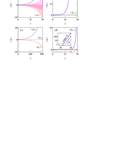
Figure 1: (Color online) (a) and (c) Evolution of the linear dimer ($\chi=0$). (b) and (d) Evolution of the nonlinear dimer ($\chi=0.5$). In panels (a) and (b) $\sigma_{\Gamma}=0.15$, $\sigma_{K}=0$, while in panels (c) and (d) $\sigma_{\Gamma}=0$, $\sigma_{K}=0.15$. In all panels $\gamma=0.25$, $\kappa=1$ and the initial conditions are $S_{0}(0)=S_{3}(0)=1$, $S_{1}(0)=S_{2}(0)=0$. The linear dynamics are obtained by means of analytical solution of system (19)-(21), while the nonlinear dynamics are obtained numerically, by averaging over $10^{4}$ realizations. In panels (a) and (c) $\langle S_{1}(z)\rangle\equiv 0$ and is not shown. The inset in (d) shows a semilogarithmic plot of $\langle S_{0,3}\rangle$ together with the straight line which represents the dependence $\propto e^{\mu z}$ with $\mu$ computed from Eq. (22).

Turning to the nonlinear dimer ($\chi>0$), we report evolution of averaged Stokes components in Figs. 1(b) and (d) which feature several interesting points. First, the figures display almost identical growths of $\langle S_{0}\rangle$ and $\langle S_{3}\rangle$ meaning that almost the whole energy is concentrated in the active waveguide. This corroborates with the fact that a deterministic nonlinear dimer obeys blowing up solutions [18, 19], and it is expectable that such (exponentially growing) trajectories dominantly contribute to blow up of the average quantities. Indeed, random fluctuations “draw” a trajectory of the dynamical system (8)-(11) to a domain of instability (reached at some propagation distance) after which the trajectory $\langle|q_{1}|^{2}\rangle$ starts growing. For sufficiently large $z$ the mean values $\langle S_{1}\rangle$ and $\langle S_{2}\rangle$ become negligibly small compared to $\langle S_{0}\rangle$ and $\langle S_{3}\rangle$. Averaging Eqs. (8) and (11) and neglecting $\langle S_{2}\rangle$, one can estimate growth rate for $\langle S_{0,3}\rangle$ in the leading order:

$$\langle S_{0}\rangle\approx\gamma Ce^{\mu z},\quad\langle S_{3}\rangle\approx\left(\sqrt{\sigma_{K}^{4}+\gamma^{2}}-\sigma_{K}^{2}\right)Ce^{\mu z},$$

where

$$\mu=4\sigma_{\Gamma}^{2}-2\sigma_{K}^{2}+2\sqrt{\sigma_{K}^{4}+\gamma^{2}}>0,$$ (22)

and $C$ is a constant. The obtained result reveals an interesting feature: if the fluctuations of the coupling are present, i.e. $\sigma_{K}>0$ [as in Fig. 1 (d)], then the average energy in the coupler arm with dissipation, i.e. $2\langle|q_{2}|^{2}\rangle=\langle S_{0}\rangle-\langle S_{3}\rangle$, grows exponentially. If, however, $\sigma_{K}=0$ [as in Fig. 1 (b)], then $\langle S_{0}\rangle$ and $\langle S_{3}\rangle$ grow with the same velocity in the leading order and the behavior of the difference $\langle S_{0}\rangle-\langle S_{3}\rangle$ is determined by the corrections of the next orders. Our numerical results for Fig. 1 (b) indicate that $\langle|q_{2}|^{2}\rangle$ oscillating slowly decreases (we could not ensure whether $\langle|q_{2}|^{2}\rangle$ eventually vanish at $z\to\infty$; either way, this issue has no physical relevance because of exponential growth of the intensity in the active arm).

Further we notice that Figs. 1(b) and (d) feature comparable scales for the growth of $\langle S_{0}\rangle$ and $\langle S_{3}\rangle$ [contrary to those in Figs. 1(a) and (c)]. Besides, the nonlinear growth of $\langle S_{0,3}\rangle$ is more rapid compared to the linear case. This indicates that the nonlinear resonances are responsible for the observed growth of the intensity. It is interesting that even though the nonlinearity is responsible for the blow-up dynamics (as discussed above), the growth exponent does not depend of the nonlinearity strength $\chi$ itself. The inset in Fig. 1(d) illustrates that the growth exponent $\mu$ obtained in (22) indeed matches the curves for $\langle S_{0}\rangle$ and $\langle S_{3}\rangle$ in Figs. 1(b) and (d).

We also notice that the nonlinearity suppresses the oscillations of $\langle S_{2}\rangle$ [c.f. Fig. 1 (a) and Fig. 1(b)].

Returning to the linear case, we proceed to the case of the broken ${\cal PT}$ symmetry ($\gamma>\kappa$) as well as for the exceptional point ($\gamma=\kappa$). The evolution of the Stokes components in the latter case is illustrated in Figs. 2(a) and (c). Comparing these two panels we observe that the effects of gain/loss and coupling fluctuations are qualitatively very similar. The quantities $\langle S_{j}\rangle$ grow faster than for the unbroken ${\cal PT}$ symmetry [Figs. 1 (a) and (c)]. Indeed, from (19)–(21) one finds that for $\gamma=\kappa$ the growth exponent is given as $\lambda_{0}\approx[8\kappa^{2}(\sigma_{\Gamma}^{2}+2\sigma_{K}^{2})]^{1/3}$, which yields $\lambda_{0}\approx 0.64$ in Figs. 2 (a) and $\lambda_{0}\approx 0.65$ in Figs. 2 (c). Similar to the case of the unbroken ${\cal PT}$ symmetry, at $\kappa=\gamma$ we observe exponential growth of the field in the arm with dissipation. However, in the nonlinear case [shown in Figs. 2(b) and (d)] the value $\langle|q_{2}|^{2}\rangle$ grows only if fluctuations of coupling are present ($\sigma_{K}>0$). For $\sigma_{K}=0$ and $\sigma_{\Gamma}>0$ the fluctuations of gain and losses result in decay of $\langle|q_{2}|^{2}\rangle$ as $z\to\infty$.

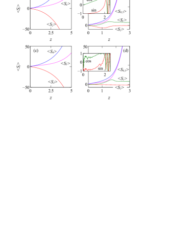
Figure 2: (Color online) The same as in Fig. 1 but with $\gamma=1$ (the exceptional point of the deterministic problem). The insets in (b) and (d) show dependencies $\langle\cos(\Delta\varphi)\rangle$ and $\langle\sin(\Delta\varphi)\rangle$ (green and red curves, respectively) for a single arbitrarily chosen realization.

Another interesting feature observed in Fig. 2 (b) is that $\langle S_{1}\rangle\to 4$ and $\langle S_{2}\rangle\to 0$ as $z\to\infty$. In order to understand this issue, let us first consider only fluctuations of the gain and losses (i.e. $\sigma_{K}=0$). From the numerics we conclude that $S_{0}$ and $S_{3}$ grow practically in a deterministic way and $\langle S_{2}\rangle\sim\langle\sin(\Delta\varphi)\rangle\to 0$, where $\Delta\varphi$ is a difference between the phases of the fields in the waveguides which is randomized due to the fluctuations (evolutions of the phases for two realizations are illustrated in insets in Fig. 2). Then, after averaging Eq. (10) one concludes that this is possible only if $\langle S_{1}\rangle\sim\langle\cos(\Delta\varphi)\rangle\to 2\kappa/\chi$ (which is equal to $4$ in all our numerics). Fluctuations of the coupling do not affect these qualitative arguments because as follows from (4) and almost deterministic behavior of $S_{3}$, the correlator $\langle K(z)S_{3}\rangle$ is of order of the fluctuations of the dispersion of $S_{3}(z)$, which is negligible.

We finally address the case of the broken ${\cal PT}$ symmetry ($\gamma>\kappa$). A typical outcome for the nonlinear system is shown in Fig. 3 (b) and (d). Comparing these results with those for the exceptional point [Fig. 2], we observe certain resemblance, in particular, in quasi-deterministic growth of $S_{0}$ and $S_{3}$ and in the asymptotic tendency of $\langle S_{1,2}\rangle$ determined by the phase mismatch of the fields in the waveguides. The main peculiarities of this case are the growth exponents, which are given by $2\sqrt{\gamma^{2}-\kappa^{2}}$ and practically identical growth of $\langle S_{0}\rangle$ and $\langle S_{3}\rangle$ meaning stronger concentration of the energy in the waveguide with gain. The insets in Fig. 3 (b) and (d) display even more regular evolution of the phase mismatch.

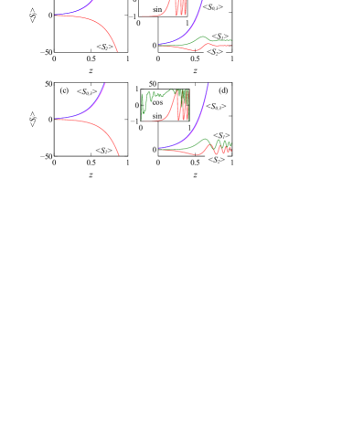
Figure 3: (Color online) The same as in Fig. 2 but with $\gamma=3$ (the broken ${\cal PT}$ symmetry of the deterministic problem).

All numerical outcomes presented above were obtained for fields applied to input of the active waveguide. We have also studied the cases when the only illuminated waveguide is the absorbing one, as well as when the input light is distributed between two waveguides. All the considered initial conditions give statistics very similar to the reported above.

To conclude, we considered field propagation in linear and nonlinear stochastic ${\cal PT}$-symmetric coupler. Our main finding is that independently on whether the ${\cal PT}$ symmetry of the underlying deterministic system is broken or not and independently on the type of fluctuations the statistically averaged intensity of the field grows. This growth is always observed in the waveguide with gain and depending on the system parameters may be observed or not in the absorbing waveguide (the latter possibility exists for the nonlinear case). The evolution of the mean field preserves the properties of the (passive) ${\cal PT}$-symmetric dynamics, where fluctuations of the gain/loss and of the coupling act respectively as the effective gain and dissipation (when they compensate each other the exact ${\cal PT}$ symmetry for the system governing the mean field is restored). As a final remark, in this Letter we left open the effect of fluctuations of the propagation constant or the effective Kerr coefficient (the latter stemming from possible imperfectness of the transverse cross-sections of the waveguides). These questions require a separate study.

VVK acknowledges discussions with Profs. A. Lupu and H. Benisty. The work was supported by FCT through the FCT grants PEst-OE/FIS/UI0618/2011 and PTDC/FIS-OPT/1918/2012.

Fifth informational page

References

- [1] C. M. Bender, Rep. Prog. Phys. 70, 947 (2007).
- [2] A. Ruschhaupt, F. Delgado, and J. G. Muga, J. Phys. A 38, L171 (2005).
- [3] W. D. Heiss, J. Phys. A 45, 444016 (2012).
- [4] A. Guo, G. J. Salamo, M. Volatier-Ravat, V. Aimez, G. A. Siviloglou, and D. N. Christodoulides, Phys. Rev. Lett. 103, 093902 (2009).
- [5] R. El-Ganainy, K. G. Makris, D. N. Christodoulides, and Z. H. Musslimani, Opt. Lett. 32, 2632 (2007).
- [6] C. E. Rüter, K. G. Makris, R. El-Ganainy, D. N. Christodoulides, M. Segev, and D. Kip, Nature Phys. 6, 192 (2010).
- [7] L. Feng, M. Ayache, J. Huang, Y.-L. Xu, M.-H. Lu, Y.-F. Chen, A. Scherer, Science 333, 729 (2011).
- [8] H. Benisty, A. Degiron, A. Lupu, A. De Lustrac, S. Chais, S. Forget, M. Besbes, G. Barbillon, A. Bruyant, S. Blaize, and G. Lérondel, Opt. Express 19, 18004 (2011).
- [9] C. Hang, G. Huang, and V. V. Konotop, Phys. Rev. Lett. 110, 083604 (2013).
- [10] C. Hang, D. A. Zezyulin, V. V. Konotop, and G. Huang, Opt. Lett. 38, 4033 (2013).
- [11] N. Bender, S. Factor, J. D. Bodyfelt, H. Ramezani, D. N. Christodoulides, F. M. Ellis, and T. Kottos, Phys. Rev. Lett. 110, 234101 (2013).
- [12] C. M. Bender, B. K. Berntson, D. Parker, and E. Samuel Am. J. Phys. 81, 173 (2013).
- [13] H. Ramezani, T. Kottos, R. El-Ganainy, and D. N. Christodoulides, Phys. Rev. A 82, 043803 (2010).
- [14] A. A. Sukhorukov, Z. Xu, and Y. S. Kivshar, Phys. Rev. A 82, 043818 (2010).
- [15] L. Cruzeiro-Hansson, P. L. Christiansen, and J. N. Elgin, Phys. Rev. B 37, 7896 (1988).
- [16] V. V. Konotop and L. Vázquez, “Nonlinear Random Waves” (World Scientific, 1994).
- [17] V. I. Klyatskin “Dynamics of Stochastic Systems” (Elsevier, Amsterdam, 2005).
- [18] P. G. Kevrekidis, D. E. Pelinovsky, and D. Y. Tyugin, J. Phys. A: Math. Theor. 46, 365201 (2013).
- [19] I. V. Barashenkov, G. S. Jackson, and S. Flach, Phys. Rev. A 88, 053817 (2013).

References

- [1] C. M. Bender, Making sense of non-Hermitian Hamiltonians, Rep. Prog. Phys. 70, 947 (2007).
- [2] A. Ruschhaupt, F. Delgado, and J. G. Muga, Physical realization of -symmetric potential scattering in a planar slab waveguide. J. Phys. A 38, L171 (2005).
- [3] W. D. Heiss, The physics of exceptional points, J. Phys. A 45, 444016 (2012).
- [4] A. Guo, G. J. Salamo, M. Volatier-Ravat, V. Aimez, G. A. Siviloglou, and D. N. Christodoulides, Observation of PT-Symmetry Breaking in Complex Optical Potentials, Phys. Rev. Lett. 103, 093902 (2009).
- [5] R. El-Ganainy, K. G. Makris, D. N. Christodoulides, and Z. H. Musslimani, Theory of coupled optical PT-symmetric structures, Opt. Lett. 32, 2632 (2007).
- [6] C. E. Rüter, K. G. Makris, R. El-Ganainy, D. N. Christodoulides, M. Segev, and D. Kip, Observation of parity–time symmetry in optics, Nature Phys. 6, 192 (2010).
- [7] L. Feng, M. Ayache, J. Huang, Y.-L. Xu, M.-H. Lu, Y.-F. Chen, A. Scherer, Nonreciprocal light propagation in a silicon photonic circuit, Science 333, 729 (2011).
- [8] H. Benisty, A. Degiron, A. Lupu, A. De Lustrac, S. Chais, S. Forget, M. Besbes, G. Barbillon, A. Bruyant, S. Blaize, and G. Lérondel, Implementation of PT symmetric devices using plasmonics: principle and applications, Opt. Express 19, 18004 (2011).
- [9] C. Hang, G. Huang, and V. V. Konotop, PT Symmetry with a System of Three-Level Atoms. Phys. Rev. Lett. 110, 083604 (2013).
- [10] C. Hang, D. A. Zezyulin, V. V. Konotop, and G. Huang, Tunable nonlinear parity–time-symmetric defect modes with an atomic cell, Opt. Lett. 38, 4033 (2013).
- [11] N. Bender, S. Factor, J. D. Bodyfelt, H. Ramezani, D. N. Christodoulides, F. M. Ellis, and T. Kottos. Observation of Asymmetric Transport in Structures with Active Nonlinearities Phys. Rev. Lett. 110, 234101 (2013).
- [12] C. M. Bender, B. K. Berntson, D. Parker, and E. Samuel Observation of PT phase transition in a simple mechanical system. Am. J. Phys. 81, 173 (2013).
- [13] H. Ramezani, T. Kottos, R. El-Ganainy, and D. Christodoulides, Unidirectional nonlinear PT-symmetric optical structures, Phys. Rev. A 82, 043803 (2010).
- [14] A. A. Sukhorukov, Z. Xu, and Y. S. Kivshar, Nonlinear suppression of time reversals in PT-symmetric optical couplers, Phys. Rev. A 82, 043818 (2010).
- [15] L. Cruzeiro-Hansson, P. L. Christiansen, and J. N. Elgin, Comment on “Self-trapping on a dimer: Time-dependent solutions of a discrete nonlinear Schrödinger equation”, Phys. Rev. B 37, 7896 (1988).
- [16] V. V. Konotop and L. Vázquez, “Nonlinear Random Waves” (World Scientific, 1994).
- [17] V. I. Klyatskin “Dynamics of Stochastic Systems” (Elsevier, Amsterdam, 2005).
- [18] P. G. Kevrekidis, D. E. Pelinovsky, and D. Y. Tyugin, Nonlinear dynamics in PT-symmetric lattices, J. Phys. A: Math. Theor. 46, 365201 (2013).
- [19] I. V. Barashenkov, G. S. Jackson, and S. Flach, Blow-up regimes in the PT-symmetric coupler and the actively coupled dimer, Phys. Rev. A 88, 053817 (2013).